Control estimates and well-posedness of an inverse subsidence problem in geomechanics

Abstract

Underground geotechnical or civil engineering works change the primary stressed and strained state of the rock mass and subsequently the fields of displacement and stresses. A significant effect of these changes is the formation of subsidence in the earth’s surface with significant negative economic or other consequences. In a series of recent works, large-scale subsidence in geostructures was modelled using Litwiniszyn’s theory (Einstein–Kolmogorov Differential Equation) and the trap-door mechanism. The solution of the Inverse Subsidence Diffusion–Convection (ISDC) problem – which belongs to the class of backward parabolic problems – provides the base (gravity-directed) displacement using the surface subsidence as ‘initial’ condition. Early well-posedness of the initial and boundary value problems has already been examined (in terms of stability estimates) in previous papers. In this work, study of control estimates and well-posedness of the ISDC problem, using energy method, are discussed.

Keywords:

• subsidence
• control estimates
• well-posedness
• diffusion–convection
• geomechanics

Classification:

• 35R30
• 35K10
• 35Q82; 35Q70; 35R25

Introduction

Underground geotechnical or civil engineering works may cause changes in the primary stressed and strained state of the rock mass. A significant effect of these changes is the formation of subsidence in the earth’s surface with significant negative economic or other consequences. According to an early work of Litwiniszyn,[1] large-scale subsidence over a yielding underground geostructure can be modelled as a stochastic Markov process. Subsequently, the distribution of subsidence, in some depth level, as a result of a displacement ‘convection–diffusion’ mechanism is calculated, under the hypothesis that subsidence is known in a greater depth of the earth’s surface. The mathematical elaboration of the model leads to a partial differential equation of parabolic type (Einstein–Kolmogorov Differential Equation) for the subsidence distribution in the geostructure (Figure 1):(2) where C is related to soil/rock properties of the geostructure.[1, 2]

Fig. 1 The trap door mechanism.

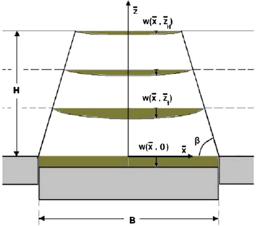
The mathematical description of subsidence due to underground works, is quite complex, owing to the large number of unknowns involved and the uncertainty of data used. As a consequence, in order to capture the phenomenon at least in a rough – but for engineering purposes, satisfactory – manner, ‘primitive’ models and solutions are employed. For instance, unknown base settlements may be replaced by the base surface average, approach naturally leading to consider the so-called trap-door mechanism (Figure 1) in lieu of the true subsidence mechanism, based on the reference paper by Terzaghi.[3]

Terzaghi’s trap-door experiment consists of a box filled with sand, where a section of the bottom can move downwards (in the direction of gravity). In order to simulate the effect of underground works in plain strain conditions the section in the bottom of the trap-door is a long rectangular plate (cf. [3, 4], Figure 1). Then, the imposed trap-door displacement is diffused upwards and, depending on the parameters of the problem, several phenomena concerning the soil mass are observed.[4, 5] The failure mechanisms that are observed during the evolution of the trap-door experiment, correspond to the trap-door mechanism.

Trap-door experiments with sand [3–5] have shown that trap-door displacements are practically convected upwards through a mechanism that localizes them above the trap-door (Figure 1). The boundaries of the subsidence trough are shear-bands, inclined inwards reducing significantly the extent of the depression in the vertical direction. As was documented experimentally, the angle of the trough boundaries varies with the trap-door displacement. In particular, it was indicated that increases with trap-door displacement; i.e. by increasing trap-door displacement, the boundaries of the trough tend to become vertical.

Using the above described trap-door mechanism, introducing a set of dimensionless variables, considering several transformations of the mathematical quantities and symmetry of the domain, the following dimensionless initial-boundary (i.-b.) value problem was obtained [2] for the subsidence distribution:(3) for(4) and ‘initial condition’ (i.c)(5) The boundary conditions (b.c.) of the problem are(6) (7) where the dimensionless variables and are connected with the horizontal and vertical coordinate , respectively,[2] H is the height of the geostructure, B is the width of the trap-door (Figure 1). In particular, if we assume that is the subsidence distribution, the equations that correlate the physical and the dimensionless quantities are the following(8) (9) The above-mentioned (Equations (2)–(6)) initial-boundary value (i.-b.v.) problem (which is defined as the Direct Subsidence Diffusion-Convection problem (DSDC),[2]) is a well-posed parabolic problem. The initial condition for the DSDC Problem is the subsidence at the base of the trap-door mechanism. Then the surface subsidence is computed using the solution of the DSDC problem. The difficulty in large-scale problems lies on the fact that for a given surface subsidence, the corresponding base displacement is not known. The problem of computing the base displacement, using the surface subsidence as ‘initial’ conditions, corresponds to the solution of the inverse in ‘time’ (depth) Subsidence Diffusion-Convection (ISDC) problem (assuming that ):(10) for(11) and(12) (13) (14) (15) This kind of problems belongs to the class of inverse parabolic problems and correspond to a Backward Diffusion-Convection problem with variable coefficients. The backward parabolic problems are in general ill-posed.[6] Furthermore, the ISDC problem belongs to the class of Inverse diffusion-convection problems in contaminant problems where few works exist [7] and additional stability considerations should be made due to the convective character of the problem.

Several methods have been developed for the regularization of Backward parabolic problems (a review is made in [8]); one class of methods involves the perturbation method. Some references on perturbation methods for parabolic problems may be found in [6, 8–19] and in references therein. As far as backward parabolic problems are concerned, Lions [9] introduced the method of quasireversibility for the solution of the backward heat conduction problem, studied well-posedness and calculated some estimates. Other efforts are including the perturbation method described in [8, 11, 12, 16] and the perturbation method described in [11, 15].

The previous mentioned methods were initially considered for the regularization of the ISDC problem. In previous works of one of the authors,[20–22] several comparisons of the previous mentioned methods, including the optimum one were presented. The method proposed by Lions provides satisfactory results (stability and convergence) only for very limited values of depth due to the strong diffusive character of the regularization term. The perturbation term proposed in [8, 11, 12, 16] provided satisfactory results (with respect to the direct solution) only for increased values of the regularization parameter . Nevertheless, the use of increased values of modifies significantly the initial model and questions the reliability of the model. Moreover, the perturbation term proposed in [11, 15], provided results that are ignoring the diffusive (expanding) character of the problem, and subsequently the divergence of the results with respect to the results of the DSDC problem, was significant.

The optimum choice was based on a method proposed by Elden,[14] in which he considered a standard inverse heat conduction problem (standard Heat Conduction equation, boundary determination, no additional conditions). It must be noticed that discussion on well-posedness and control estimates of inverse parabolic problems, using the Elden’s method (and other perturbation methods), is also mentioned in [17–19]. Nevertheless, these works are concerning quantitatively different kinds of problems (non-standard Heat Conduction equation, constant coefficients, boundary determination, no additional conditions).

The optimum regularization for the ISDC problem is presented below (as described in [20]):(16) for(17) and(18) (19) (20) (21)

Fig. 2 Comparison of DSDC problem and inverse subsidence diffusion–convection problem results using regularization [20].

It can be observed that, compared with the the direct problem, the difference in the initial conditions is concerning the i.c. Equation (20). This constitutes a significant improvement, since it is (in general) possible not only to measure the profile of the surface subsidence (Equation (17)), but also to estimate the profile of the subsidence close to the free surface, using some shallow depth recognizance technique. Thus, it is in general possible to acquire the data described in Equation (20).

The results of the Direct and the regularized Inverse problem (optimum regularization) are presented in Figure 2, in the form , for both problems. The data that have been used correspond to Test-1, as referred in [2], (, , and ) and introduced in [5]. Initially, the DSDC problem is solved until a certain normalized height (which correpsonds to a value). Then, the results of the DSDC problem are used as initial conditions and b is replaced by in the Equations of the regularized ISDC problem. Both solutions are then plotted in the corresponding Figure, (Figure 2).

Stability of the numerical algorithm using Fourier method and the von Neumann condition, as well as the convergence of the numerical and the exact solution, using truncation error, was examined for all the regularization methods used for the ISDC and subsequently for the optimum regularization method, . According to the von Neumann condition, stability of the numerical algorithm is ensured due to right choices of the regularization parameter and geometrical parameter b of the problem that influence the quantity .[20, 23] Convergence in terms of truncation error is satisfactory, except for the boundary x=1, where all the regularization methods have significant differences with respect to the solution of the direct problem.[20–22] Linear stability analysis, using Fourier method has been also examined and some estimates were addressed.[23]

In this work, interest is focused on the discussion of control estimates and well-posedness of the ISDC problem. Initially, some control estimates are provided for the optimum regularization of the ISDC problem. Then, by neglecting the first-order derivative in , a more simplified estimate is calculated and the limitations of the approach are discussed. Well-posedness is discussed in terms of energy method; subsequent considerations are provided in a separate subsection.

Control estimates – method 1

Originally, some definitions and simplified equations are given concerning the initial and boundary value problem Equations (15)–(20): we define as and (functions of and respectively) the variable coefficients of the Partial Differential Equation (Equation (15))(22) (23) Furthermore, the inner product on is defined as:(24) Then the weak formulation of the above-mentioned i.-b. value problem is: we seek where(25) Precise definition of the weak solution can be given by adopting Evans’ approach [24] in Section 7.2.

Energy estimates

It should be noticed that the mathematical considerations used in this subsection were previously introduced in [25, 26] for the analysis of the wave equation.

Let where(26) Integration of Equation (24) from 0 to provides (notice that is independent of x)(27) Every term of Equation (26) is then evaluated as follows: the first part using the definition of and considering that(28) since(29) is estimated as follows:(30) The first term of the right-hand side of Equation (29) is one of the terms to be estimated. The other terms can be calculated using the initial and boundary conditions. The third term can be derived using the following Equation:(31) Since(32) for one has:(33) The second term of Equation (26) is estimated using the equation(34) which provides the following result(35) The first term of the right-hand side of Equation (34) can be calculated using the i.-b. conditions. The second term, will be derived later in this work. The third part of Equation (26) yields that(36) Summarizing the elaboration of Equation (26), the following result is obtained(37) Efforts will now be given on the elimination of . Since(38) it follows that(39) Now, using the Cauchy–Schwartz inequality, we obtain(40) Another part of Equation (36) is estimated as follows:(41) using the mean inequality for . The second part of the right-hand side of Equation (40), using Equation (31), yields that(42) Summarizing the discussion for Equation (36) one has,(43) Therefore, if we assume that we eliminate the second part of the left hand side of Equation (42) and we derive(44) In order to estimate we use Gronwall Lemma [27] as follows:

Lemma 2.1

Let with(45) where(46) and(47) then(48)

Thus, the estimation of is described by the following equation:(49) It can be seen that control estimates have significant dependence on the second part of Equation (46). If we now consider again Equation (40), we observe that(50) According to Equations (16), (22), (25), it follows that and . Physical observations indicate that is negative, as it can be also observed in .[2, 20] If the stability of the numerical algorithm is ensured, both for the diffusive and the convective character of the problem, for some , perturbations are disregarded and . Therefore, it is reasonable to assume:

Assumption 3.1

Assume thatfor all and

If Assumption 3.1 holds then(51) Consequently, Equation (36) yields that(52) and subsequently one has(53) Finally, the estimation of is improved, since in that case we obtain(54) In order to derive estimates for from estimates on , we use standard Sobolev inequalities on yielding control in and by the norm:(55) (56) In fact, these inequalities can be proved by observing that for being a continuous differentiable function with , we have and(57) Finally, using Equation (55) we obtain that(58) where and are defined in Equations (45) and (53), respectively. The right-hand part of Equation (57) will be considered as ES1 in Figure 3.

Existence-uniqueness

Following the approach of Evans,[24] Section 7.2, the key ingredient in proving existence and uniqueness of solution for the i.-b.v. problem Equations (15)–(20) is an energy bound. In fact Equation (57) yields uniqueness, since for two different solutions the difference will be also a solution to our problem with zero data. Then Equation (57) still holds and implies .

For existence of a solution, one may adopt in a straightforward manner the proof of Evans,[24] Theorem 3, p. 384 based on Galerkin approximation, still using the stability (energy) bound, Equation (57).

Remark – method 2

We now consider a simplified version of the i.b. value problem Equations (15)–(20). Equation (15) can be rewritten in the form:(59) where and are described in Equations (21) and (22). If the part of the equation that involves the first derivative due to is ignored, then Equation (58) is transformed in the following Equation(60) It must be noticed that in the following calculations, is considered parameter with values defined by Equations (16) and (21). In this point, we must mention that numerical results have shown that for the central subsidence () the influence of the first-order term is negligible(61) where is the solution of the i.-b. value problem Equation (59), (16)– (20). Let denote the standard Sobolev space of elements of with weak derivatives up to the order in Let the elements of which are zero at In this point we define operator on as follows:(62) Then Equation (59) is equivalent to the following:(63) and subsequently(64) where is the inverse operator of . Using an additional equation for , the following system of equations is obtained:(65) A simplified manipulation of the later equation provides that(66) Therefore, since , one has(67) According to the Gronwall Lemma [27], we finally derive that(68) The right-hand side of Equation (67) corresponds to a more simplified estimation than ES1, which is referred as ES2 in Figure 3. The right part of Equation (67) can be considered as estimate of , since:  . it maximizes the estimates for in any case and . the maximum of is obtained for (), where .[2]

The estimation described from Equation (67) can be used in the cases where the first derivative has not significant influence on the numerical results. This is translated in small values of c, which are observed for loose soils and/or decreased width of the trap-door (see Equations (1), (7) and (8). In a rough manner, for values of c greater than 0.15, the influence of the first-order derivative is negligible. It should be also noticed that according to the data used, the maximum subsidence is observed in (central subsidence). The approximated solution of the i.-b.v. problem Equations (58), (16)–(20) provides very similar results with the regularized ISDC problem, for the central subsidence.

Comparison-results

The well-posedness of the i.-b. value problem Equations (15)–(20) is already discussed in a previous section. In the following paragraphs, a comparison of the results of the different estimates is presented. If we consider the numerical results of the corresponding i.-b.v. problems using the data provided in a previous section (, , and ),[2, 5] and define(69) where OES is the observed amplification factor of the numerical solution, then the results are presented in Figure 3, in logarithmic scale with respect to the regularization parameter . Quantitatively similar results are obtained if the estimates are normalized with respect to the imposed – as an initial condition of the direct problem – value of subsidence .

Fig. 3 Comparison of inverse subsidence diffusion–convection problem results for and .

It can be easily verified that as tends to 0, the i.-b. value problem Equations (15–20) is tending to the i.-b. value problem Equations (9)–(14) which is an ill-posed problem. This comment can be also confirmed from the estimates, since for approaching zero the estimates Equations (57) and (67) are tending to infinity. If we increase the values of , the problem becomes well-posed but greater values of lead to another model, with questionable reliability, as already mentioned in the Introduction.

It can be also observed that for small values of , the simplified method Equation (67), provides better estimates (Figure 3, left). On the contrary, for increased values of the maximum height, the estimates provided in Equation (57) are providing improved results (Figure 3, right).

Finally, it must be pointed that – as explained in the corresponding section – the simplified method can be used with some limitations in contrast with the earlier one, which can provide estimates in any case.

Conclusions

In summary the following propositions are inferred:

•	Well-posedness for the optimum -regularization is ensured using energy methods.
•	The simplified method provides better estimates than those obtained from the more general method for small values of the maximum height and particular values of . On the contrary, the more generalized method derives better estimates for any other case.

 

i.	horizontal cartesian coordinate
ii.	vertical cartesian coordinate – direction of gravity
iii.	subsidence distribution
iv.	normalized horizontal coordinate
v.	normalized vertical coordinate
vi.	normalized vertical coordinate for the inverse problem
vii.	maximum value of that the regularized inverse problem is solved
viii.	maximum normalized height that the direct problem is solved
ix.	equals to
x.	(positive) constant coefficient of diffusion in the Litwiniszyn’s model
xi.	depending on soil/rock properties
xii.	dimensionless diffusive constant depending soil conditions and geometry
xiii.	normalized subsidence distribution for the direct problem
xiv.	normalized subsidence distribution for the inverse problem
xv.	height of the geostructure
xvi.	width of the trap-door
xvii.	inclination angle that determines the boundaries of the domain of subsidence
xviii.	variable width of the boundary of the domain (with height)
xix.	normalized subsidence distribution for the regularized inverse problem
xx.	partial derivative due to for
xxi.	regularization parameter
xxii.	variable coefficients of the regularized partial differential equation (15)
xxiii.	first derivative of with respect to
xxiv.	solution of the regularized inverse problem Equations (59, 16–20)
xxv.	auxiliary function used in the simplified estimation defined as
xxvi.	numerical approximation of at and
xxvii.	the standard space of integrable and measurable functions on (0, 1), such that
xxviii.
xxix.	the standard inner product on defined as
xxx.	the standard norm defined as
xxxi.	the standard Sobolev space of elements of with weak derivatives up to the
xxxii.	order in
xxxiii.	the elements of with trace at
xxxiv.	the operator on defined as
xxxv.	the inverse operator of on defined as
xxxvi.	for . It is a function of .
xxxvii.	constant value between 0 and
xxxviii.	auxiliary function
xxxix.	auxiliary variables
xl.	constant value concerning the Cauchy–Schwartz inequality
xli.	auxiliary functions used in Gronwall’s Lemma
xlii.	auxiliary functions used in Gronwall’s Lemma
xliii.	auxiliary functions

Acknowledgments

The first of the authors would like to dedicate this work to the late Professor Ioannis Vardoulakis.

References

- Litwiniszyn, J, 1974. Stochastic methods in the mechanics of granular bodies. Wien: Springer-Verlag; 1974.
- Vardoulakis I, Vairaktaris E, Papamichos E. Subsidence diffusion-convection: I. The direct problem. Computer Methods in Applied Mechanics and Engin. 2004;193:2745–2760..
- Terzaghi Kv. Stress distribution in dry and saturated sand above a yielding trap-door. Proceedings of the International Conference on Soil Mechanics. Vol. 1; Cambridge (MA); 1936. p. 307–311..
- Vardoulakis I, Graf B, Gudehus G. Trap-door problem with dry sand: a statical approach based upon model test kinematics. Int. J. Numer. Anal. Methods Geomech. 1981;V:57–78..
- Papamichos E, Vardoulakis I, Heil LK. Overburden modeling above a compacting reservoir using a trap door apparatus. Phys. Chem. Earth Part A. Solid Earth and Geod. 2001;26:69–74..
- Dang, DT, and Nguyen, HT, 2006. Regularization and error estimates for nonhomogeneous backward heat problems, Electron. J. Diff. Eq. 4 (2006), pp. 1–10.
- Pektas, B, 2009. Modeling and computer simulation of the identification problem related to the sludge concentration in a settler, Math. Computer Model. 49 (2009), pp. 843–855.
- Han, Z, Huang, Y, and Jian, M, 2010. "Inverse problems for equations of parabolic type". In: Yang, Y, Fu, X, and Duan, J, eds. Perspectives in mathematical sciences (Interdisciplinary Mathematical Sciences). Singapore: World Scientific; 2010. pp. 93–113.
- Lattes, R, and Lions, JL, 1969. The method of quasi-reversibility. New York (NY): American Elsevier; 1969.
- Lavrentiev, MM, 1973. Some improperly posed problem of mathematical physics, Springer Tracts in Natural Phil. 11 (1973), pp. 161–171.
- Miller K. Stabilized quasi-reversibility and other nearly-best-possible methods for nonwell- posed problems. In: R.J.Knops, editor. Lecture notes in mathematics. Symposium on Non-Well-Posed Problems and Logarithmic Convexity, Heriot-Watt University, Berlin: Springer; 1973. p. 161–176..
- Payne, LE, 1973. "Some general remarks on improperly posed problems for partial differential equation". In: Knops, RJ, ed. Lecture notes in mathematics. Symposium on Non-Well-Posed Problems and Logarithmic Convexity, Heriot-Watt University, Berlin: Springer; 1973. pp. 1–30.
- J. Math. Anal. Appl. The final value problem for evolution equations. 1974;47:563–572..
- Elden, L, 1987. Approximations for a Cauchy problem for the heat equation, Inverse Prob. 3 (1987), pp. 263–273.
- Lesnic, D, Elliott, L, and Ingham, DB, 1998. An iterative boundary element method for solving the backward heat conduction problem using an elliptic approximation, Inverse Probl. Engin. 6 (1998), pp. 255–279.
- Ames, KA, and Payne, LE, 1999. Continuous dependence on modeling for some well-posed perturbations of the backward heat equation, J. of Inequal. and Appl. 3 (1999), pp. 51–64.
- Qian, Z, Fu, C-L, and Xiong, X-T, 2006. A modified method for a non-standard inverse heat conduction problem, Applied Mathematics and Comp. 180 (2006), pp. 453–468.
- Qian, Z, and Fu, C-L, 2007. Regularization strategies for a two-dimensional inverse heat conduction problem, Inverse Prob. 23 (2007), pp. 1053–1068.
- Qian, Z, Fu, C-L, and Xiong, X-T, 2007. Modified method for determining the surface heat flux of IHCP, Inverse Problems in Science and Engin. 15 (2007), pp. 249–265.
- Vardoulakis, I, Vairaktaris, E, Papamichos, E, and Dougalis, V, 2004. Subsidence diffusion-convection: II. The inverse problem, Comput. Methods Appl. Mech. Eng. 193 (2004), pp. 2761–2770.
- Vardoulakis I, Vairaktaris E, Papamichos E, Dougalis V. Contribution to the inverse subsidence diffusion-convection problem in geostructures. Proceedings of 2nd Workshop for young doctors in Geomechanics; Paris. Vol. 1. 2002; p. 41–44..
- I. Vardoulakis, E. Vairaktaris, E. Papamichos, and V. Dougalis, Modeling the Inverse Subsidence Diffusion-Convection in Geostructures, Proc. of the 4th International Conference on Inverse Problems in Engineering: Theory and Practice, Angra dos Reis, Brazil. I (2002), pp. 326–333..
- Vairaktaris E. Study of the direct and inverse subsidence diffusion - convection problem in geostructures [Phd Thesis]. Greece: NTU of Athens; 2003. (in Greek)..
- Evans, LC, 1997. Partial differential equations, graduate studies in mathematics. Berkeley (CA): American Mathematical Society; 1997.
- Ladyzhenskaya, OA, 1985. The boundary value problems of mathematical physics, applied mathematical sciences. Berlin: Springer Verlag; 1985.
- Baker, GA, 1976. Error estimates for finite element methods for second order hyperbolic equations, SIAM J. Numer. Anal. 13 (1976), pp. 564–576.
- Makridakis C. Numerical methods on Galerkin/finite elements for the equations of elastodynamics [Phd Thesis]. Greece: University of Crete; 1989 (in Greek)..