Retrieve properties of participating media by different spans of radiative signals using the SPSO algorithm

Abstract

The numerical model of a short-pulse laser propagating in participating media was analysed based on the complete transport theory described as the transient radiative transfer equation (TRTE). The finite volume method was used to solve the TRTE for any dimensional problem. Radiative signals are transmitted signals and reflected signals caused by time-domain laser pulse and signal results were compared with the benchmark results obtained by the reverse Monte Carlo method. Moreover, sensitivity analysis has been presented with different thickness, short pulse width and optical properties. In order to estimate the optical parameters effectively, some criteria for choosing more sensitive spans of the measured signals have been obtained based on the sensitivity analysis. Furthermore, different sampling spans and peak values of radiative signals were used as measurement data for inverse analysis by using the stochastic particle swarm optimization algorithm. Firstly, the different sampling times of transmittance and reflectance signals were, respectively, used as the measurement data to reconstruct optical properties (scattering coefficients and absorption coefficients) of one-dimensional participating media. After that, the maximums of the signals for inverse analysis with different albedos were investigated and the properties of different cases were estimated and listed.

Keywords:

• TRTE
• short-pulse laser
• sampling spans
• inverse problems
• SPSO

1. Introduction

In recent years, optical methods using near-infrared light (NIR) in applications of semi-transparent media have become a promise and increasingly important for non-invasive diagnostics in medicine. In these methods, the preferred range for optical tomography (OT) is between 600 and 900 nm, that is at the frontier of the visible range and the NIR region of the electro-magnetic spectrum, which is the region of the highest physiological transitivity, and it is the optical communication gateway for the laser energy to propagate into the human body. Moreover, electro-magnetic beam in this region is not used for imaging directly, but only for its interaction with the semi-transparent media (such as human tissues), based on their local optical properties.[1] In fact, the optical properties of turbid media such as clouds, fog, water media and biological tissues are spatially inhomogeneous. The inhomogeneity is statistical to some degree, which leads to the necessity of the statistical description of light fields in such media, in particular the absorption coefficients and refractive index.[2–5]

When optical properties of the object to be probed are addressed, a signature of the matter can be obtained. Then, a specific alteration of the tissue can be identified. The reason is that OT exploits the fact that various disease processes, physiological changes or simply contrasts between zones of different nature are identified through their optical properties (mainly absorption coefficients and scattering coefficients).[6] Light propagation within biological media is accurately described by the radiative transfer equation (RTE) and it is widely used in the biomedical imaging bioluminescence tomography,[7,8] while the short-pulse laser transmission inside semi-transparent media is described by the transient radiative transfer equation (TRTE). OT is an inverse problem which consists in identifying the parameters of a numerical model based on the radiative transfer equation from surface measurements by using a minimization of the mean-square discrepancy between the measurements and the predictions of the forward model.

Based on the TRTE, in order to reconstruct the optical properties inside the semi-transparent media, three essential parts must be contained.[9] One part is a forward model that predicts the detector readings based on solutions of the diffusion theory equation or the transport theory equation. The second is an objective function that provides a measure of the differences between the detected and the predicted data. The last is the reconstruction technique which can minimize the objective function to get new guesses of the optical properties. Foremost, the basic premise is that the forward model must be solved precisely enough so that the measurement data obtained by detectors may be simulated. Consequently, in forward model, the TRTE based on the complete transport theory should be accepted. Unlike the commonly applied diffusion approximation, the TRTE accurately describes the photon propagation in turbid media without any limiting assumptions regarding the optical properties. For the participating media that contain void-like regions with very low absorption and scattering coefficient (such as cerebrospinal fluid layer or synovial fluid in joints), the diffuse approximation fails to describe light propagation in these regions accurately.[10,11] This phenomenon in which turbid media are surrounded by the sub-transparent (low scattering) media more often occurs in the biological tissues.[12] For these cases, it is highly desirable to have a reconstruction code that is based on the complete formalism of the TRTE. On the other hand, how to discretize the unsteady term of the TRTE has very important effects on the accuracy of the forward calculation. So, it is important to analyse the precision of different time-difference schemes and compare the results with those of benchmark methods. There have been several investigations into the interaction of ultra-fast radiation with participating media. In these studies, both homogeneous and inhomogeneous media have been considered. Many studies on simple one-dimensional (1-d) planar geometry [13,14] and a few on 2-D [15,16] and 3-D geometries [17,18] have been reported in the literature. However, almost all the studies used fully implicit scheme for discretizing the time term.

Generally speaking, the methods for solving the inverse radiation problems are classified into two groups. One sort is gradient-based optimal methods such as Levenberg–Marquardt algorithm and the conjugate gradient descent method and the other is search-based optimization methods such as the genetic algorithm and particle swarm optimization (PSO) based methods. PSO algorithm, first introduced by Kennedy and Eberhart,[19] may find global optimum solutions or good approximate solutions. In nearly a decade, many PSO-based methods were widely developed; for example, the stochastic PSO (SPSO) algorithm,[20,21] multi-phase PSO (MPPSO),[22,23] repulsive PSO (RPSO),[24,25] and multi-objective PSO (MOPSO),[26] etc. PSO algorithms were first introduced into transient radiative inverse problems in reference,[27] and the information inside of 1-d media were successfully reconstructed using PSO algorithms. In the present work, the SPSO method, one of the PSO-based algorithms, was used to analyse the transient radiative inverse problems. The SPSO algorithm was developed by Cui and Zeng [19,20], which can avoid premature convergence and ensure the overall convergence. The basic idea of SPSO method is the usage of a stopping evolution particle to improve global searching ability. In our previous work [27], the PSO-based algorithms were introduced in the study of transient radiative inverse problems. The radiative signals with long spans (from start to end) were used to estimate optical parameters (absorption coefficients and scattering coefficients) of the homogenous and inhomogeneous media. In the present work, in order to retrieve the medium parameters efficiently and correctly, we focus to study the effects of different sampling time for the parameter estimation and try to get the optimum sampling spans. The innovation of this work could be summarized as following: (1) the criteria for choosing more sensitive spans of the measured radiative signals (reflected signals and transmitted signals) have been presented; (2) the different sampling spans of radiative signals were investigated using the SPSO algorithm and the criteria for choosing the sensitive spans were validated; and (3) the radiative signal peak values could be used to estimate correctly the optical parameters of the homogenous media, especially for the media with high albedo.

In the following sections, detailed mathematic formulation and computational steps are given first. The present model is verified by a benchmark solution. The temporal profiles of laser pulses are considered to be step functions. The finite volume method (FVM), with a differential factor of the transient term, was used to analyse the problem. The simulation for inverse problems of transient radiative signals of long duration requires large CPU consumption. Then, under the condition of satisfying with the precision requirement, how to choose the sampling time of radiative signals has an important significance on the efficiency of the inverse calculation. In the present work, it is attempted to use the transient radiative information, i.e. different sampling spans or peak values of the radiative signals as the measurement data to estimate the optical properties of the participating media. Firstly, the sensitivities for optical properties with respect to different radiative signals (i.e. transmittance and reflectance signals) were studied. Thus, the different spans, used to retrieve the optical properties and the distance of the two-layer interface, were investigated using SPSO algorithm in the inverse problems of the 1-d media. The optimum span of sampling time was found in 1-d uniform and 1-d two-layer media. At last, the maximums of the radiative signals were studied for uniform media with different albedos and influences of optical properties (absorption and scattering coefficients) on the objective function were investigated. Moreover, the estimated results for different albedo cases were obtained only using signal peak values with the SPSO algorithm.

2 The transient radiative equation

The TRTE can be briefly written as:(1) where radiative intensity I is the function of position s, solid angle and time t; , and are extinction, absorption and scattering coefficients, respectively. In the transient problem caused by collimated irradiation, as shown in Figure 1, the radiative intensity within the medium was separated into two parts [28]: (a) the remnant of the collimated beam after partial extinction, by absorption and scattering, along its path and (b) , a diffuse part, which is the result of emission from the boundaries, emission from within the medium and the radiation scattered away from the collimated irradiation. Thus, this can be written as(2)

Consider that the collimate light cannot be refracted on the interface. Thus, the change in the collimated intensity can be found by the contribution from emission in the medium as follows:(3)

For one single step short pulse, the collimated radiative intensity can be written as(4) where is the geometric distance in the direction . is the heat flux of incident laser at boundary . is the Heaviside function, defined as(5) and is the Dirac delta function, defined as(6) and(7) Substituting (2) and (3) into (1), it can be written as(8) (9) (10) is the total source term in Equation (5a). The source term and result from collimated radiation and diffuse radiation , respectively. In the case of a diffuse reflection boundary, the boundary conditions are given by [29](11) where and are, respectively, the outgoing and the incoming intensities at the boundary, is the outward unit normal vector at the boundary and is the emissivity of the boundary. The linear anisotropic phase function in the source term can be given by(12) where , i.e. corresponding polar angles are the included angles of x axis with and direction, respectively.

Using the finite difference schemes, can be written as follows:(13) where and represent the present time step and previous time step, respectively; is a fraction from 0 to 1, when is 0, 1, 1/2 and 2/3, which represent explicit scheme, implicit scheme, Crank–Nicolson scheme and Galerkin scheme, respectively. Using the length dimension, time and is the velocity of light. Equation (5a) can be expressed as(14)

For simplicity of notation, it can be obtained from Equations (8) and (9) that(15) where and represent the present time step and the previous time step, respectively.

Equation (10) multiplied by , can be simplified as(16) where , ,

For a discrete direction and integrating it over the elemental solid angle and the control volume , we can get(17) where(18) (19) , and are the side areas of the control volume; the superscripts U and D designate upstream interface and downstream interface of the control volume, respectively; is given by(20) where is the outward unit normal of a surface of the control volume as shown in Figure 2 and is the direction along which radiation transfer happened.(21) (22) where is the symbol for the surfaces of the control volume and j represents e, w, s, n, t or b, as shown in Figure 2.

Figure 2 Control volume in the Cartesian coordinate system.

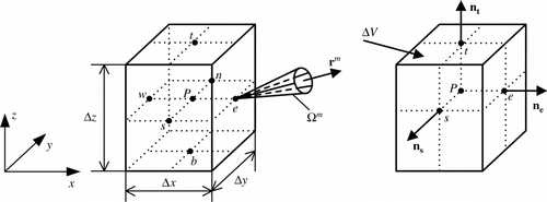
Figure 1 Three-dimension model that the participating media irradiated by the short pulse laser.

In any discrete direction , the intensity at the control volume centre is related to the surface intensities as(23) where is the finite-difference weighting factor.

Substitute (18) into (14) and eliminate the intensity terms of the downstream points. Then, the diffusion intensity for the control volume in the direction at time step can be written as(24) where subscript i represents x, y and z.

The transmittance signal and reflectance signal can be expressed as(25) (26) where is the direction cosine and is the direct transmission flux of the collimated light. In this paper, the transmittance or reflectance signal will be simulated for 1-d medium cases.

3 The inverse principle of SPSO algorithm

PSO-based approaches are similar to other evolution methods containing the conception of swarm and evolution and working based on the fitness values of particles. The flocking population is called a swarm and the individuals are called particles. The difference between PSO and other evolution methods is that each particle is considered as one particle without gravity and volume flying in n-dimensional search space and the flying velocities are fixed by the experiences of individuals and flocking population. In summary, PSO is an adaptive and robust parameter-searching technique inspired by social behaviour simulations of flocking birds. To avoid premature convergence of standard PSO and ensure the overall convergence, a SPSO algorithm was developed by Cui and Zeng [19,20]. The basic idea of SPSO method is the usage of a stopping evolution particle to improve global searching ability. In our previous paper,[27] we have studied the difference of PSO, SPSO and MPPSO algorithms for transient radiative inverse problems. It could be concluded that the SPSO algorithms could estimate the properties of the participating media more correctly than other two PSO-based algorithms for many cases. Therefore, the SPSO algorithm was used for inverse analysis in the present work. The basic idea of SPSO can be described simply as follows.

In order to describe clearly, the evolution equation of the basic PSO should be given. Based on the basic PSO model, velocity and position of an ith particle at generation t + 1 could be expressed as follows:(27) (28) where c₁ and c₂ are two positive constants called acceleration coefficients (in the present work, both c₁ and c₂ were set as 1.0); r₁ and r₂ are uniformly distributed random numbers in the interval [0,1]; is the present location of particle i, which represents a potential solution; is the present velocity of particle i, which is based on its own and its neighbours’ flying experiences; and is the “local best” during the tth generation of the swarm. The global best position of the swarm is expressed as is the “global best” up to the current generation among all the particles in the swarms. The inertia weight coefficient w is used to regulate the present velocity and it influences the trade-off between the global and local exploration abilities of particles.

In Equations (22) and (23), when is 0, the velocity of ith particle for the generation t + 1 only depends on three parameters of the previous generation t, i.e. the position , the historical best position of the ith particle and the historical best position of particle swarms. However, the velocity has no memory itself. The particles which are at the global best position will remain at rest, while other particles will fly to the weighted centre of their local best position and the global best position. In other words, particle swarms will retract to the current global best poisons, and this is more like a local algorithm. When unequal to 0, it makes particles to possess the trend of expanding the searching space (i.e. possessing certain global searching ability). Meanwhile, larger the coefficient , better global searching ability the algorithm.

Under the above analysis, when is 0, the following equation can be obtained based on Equations (22) and (23).(29)

Compared with the basic PSO algorithm, the evolution equation of Equation (24) reduced the global searching ability, but increased the local searching ability. To improve the global searching ability of Equation (24), could be retained as the historical best position and the position of particle j is generated randomly in the search space, while other particles with the position have evolved in terms of Equation (24). In this way, the following updating procedure is obtained:(30)

Once the updating procedure of Equation (25) has been completed, a test is performed:

1.	If , then the particle j generated randomly is at the historical best position. Then, it cannot evolve by Equation (24) and it will continue to be generated in the searching space, while other particles will evolve after updating and ;
2.	If and is not updated, then all particles will evolve in terms of Equation (24);
3.	If and is updated, then it means that there is k () such that , then the particle k will stop evolution and regenerated in searching space, while other particles will evolve after updating and .

So, at certain generations in the evolutionary procedure, there is at least one particle satisfying the condition of . In other words, there is at least one particle that needs to be generated randomly in the searching space so that it will certainly strengthen the global searching ability. This algorithm obtained from the basic PSO is called SPSO. The convergence procedure of SPSO is analysed in detail in reference [20,21] and it will not be repeated here.

The parameters’ setting for PSO-based algorithms, such as particle population M, maximum fly velocity V_max and size of searching space , were studied in our previous work [27] and it will not be repeated here. In the present study, the population M and the maximum fly velocity V_max were set as 50 and 1, respectively. The size of searching space was chosen in terms of the specific cases. In the searching procedure, the new velocity and the position of all particles were calculated repeatedly using Equations (24) and (25). Meanwhile, the best position and were updated until the number of cycles reaches a user-defined limit, or until the best fitness function is less than a given small value.

Transient radiative inverse problems for estimating media inside properties are solved by minimizing the objective function. The minimization of the objective function is named as the fitness function. The objective function can be defined as(31) where are the measured time-resolved transmittance or reflectance signals ( or ), which will be simulated by the forward model using the FVM and are the estimated time-resolved transmittance and reflectance for an estimated vector . Moreover, and are start and end of the sampling span, respectively. Next, the influence on the estimated results, i.e. the absorption coefficients and the scattering coefficients with different sampling span time (), will be investigated.

To demonstrate the effects of measurement errors on the predicted terms, random errors are considered. In the present paper, the radiative signals used as data for the inverse problem are obtained by adding normally distributed errors to reflectance and transmittance signals simulated with the forward problem, as shown below:(32) where is a normally distributed random variable confined as with 99% confidence. is the standard deviations of the measured value and is the measurement error. Using inverse analysis, the absorption and the scattering coefficients or the interface location of two-layer media can be estimated by minimizing the objective function using SPSO algorithms. SPSO is adopted for the minimization of the objective function, which is called the fitness function. The stop criterion of the SPSO method is that the maximum number of iteration (generation) set a priori is reached or the best fitness function is less than a specified small value.

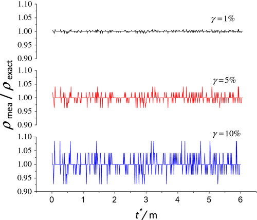
The radiative signal is the function with respect to the length dimensional time (Equations (20) and (21)). Therefore, the ratios of measured signals over the exact signals are also with respect to . The ratios of to with the noises of , 5% and 10% are shown in the Figure 3 and the total time is 6.0 m. . As shown in Figure 3, when the noise is 1%, 5% and 10%, the values of are in the intervals of (0.99, 1.01), (0.95, 1.05) and (1.10, 0.90), respectively.

Figure 3 The ratios of measured signals to the exact signals with the noises of  = 1, 5 and 10%

4 Results and discussion

Previously, our group had finished the finite-element method (FEM) code and it was in excellent agreement with other methods.[30–32] However, the main defect of FEM is that it is badly time-consuming,[27] especially in multi-dimensional models. Now, the FVM is used to analyse the short-pulse laser propagation in 1-d media as follows.

4.1 Forward results for homogeneous media cases

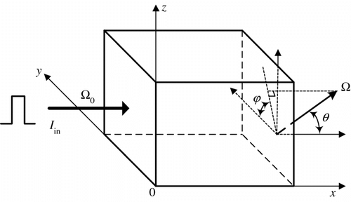
Consider that one side of a 1-d uniform semi-transparent slab with thickness L of is irradiated by a collimated step-pulse laser beam in the x-direction with pulse width of 0.1 m. The absorption coefficient is 0.02 m⁻¹ and the scattering coefficient is 9.98 m⁻¹. The emissions from the medium are neglected. Further, to simplify the situation, black boundaries of the medium are considered and the sample is an isotropic scattering medium. About 100 equal-size control volumes and solid angle elements were used. The finite-difference weighting factor were set as 1.0 (i.e. the step scheme was used). The length-dimensional time step is 0.01 m; the total length dimensional time span was divided into 1000 equal steps. So, the total length dimensional time is 10 m and at each time step , the iteration stop criterion is . (Table 1)

Table 1. Parameter settings of homogeneous cases are used in the forward models.

Test No.	α			a			Δt^∗ (m)	Meshing	Ka (m^−1)	δs (m^−1)	tp^∗^(m)
Test 1		1.0		−0.9	0	0.9	0.01	100	0.02	9.98	0.1
Test 2	0.5	0.667	1.0		0		0.01	100	0.02	9.98	0.1

In Test 1, the time differential factor is set as 1.0 (i.e. the fully implicit scheme) and the anisotropic scattering phase function is selected using corresponding to backward, isotropic and forward scattering, respectively. Test 1 was used to validate the availability of FVM procedures and this work has been accomplished in our previous research.[27] In Test 2, three different schemes, i.e. Crank–Nicolson (C-N) scheme (), Galerkin scheme () and implicit scheme () will be studied. For the sake of simplicity, only the isotropic scattering medium (a = 0) was studied. In order to study the accuracy of different time schemes, the length dimensional time step was set as a relatively large value of 0.1 m. Using a relatively large value of the time step is conducive to improve the computing efficiency of the inverse problems, as it will certainly influence the computational accuracy. As shown in Figure 4, the results of the three schemes were compared with the reverse Monte Carlo method (RMC) method, which is considered as a benchmark result. It can be seen from the Figure 4 that when the length dimensional time step is 0.1 m, the result predicted by FVM with Galerkin scheme () agrees with the benchmark solution of RMC method better than other time-difference schemes. Thus, it is suggested that simultaneously using Galerkin scheme and relatively large value () of time step could improve the estimated efficiency under the condition of ensuring accuracy.

Figure 4 Solutions of Test 2 from the present work and RMC methods [33] are compared.

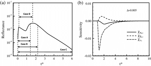
4.2 Sensitivity analysis

In function estimation, as in parameter estimation, a detailed examination of the sensitivity coefficients can provide considerable insight into the estimation problem. In order to get more quantitative information of the different sampling spans of the transmittance or reflectance signals, the sensitivity with respect to the unknown parameters (absorption and scattering coefficients) should be studied first. The sensitivity coefficient is defined as the first derivative of a dependent variable, which is the radiative signal in the present work. One finite-difference approximation for the sensitivity for the jth radiative signal, kth parameter is the forward-difference approximation or the central difference scheme. When the parameter equals , sensitivity coefficients are defined as follows:(33) where represents the absorption or scattering coefficients; is the tiny change percentage of the parameter. So, the sensitivity coefficients and are the first derivatives of the transmittance or reflectance signal at time with respect to and , respectively. If the sensitivity coefficients are small, the estimation problem is difficult and very sensitive to measurement errors.

4.2.1 Sensitivity coefficients with different thicknesses (L) and pulse width ()

In order to study the influences of the thicknesses L and pulse width on the sensitivity coefficients, one 1-d homogenous medium was considered with the absorption coefficient of 1.0 m⁻¹ and scattering coefficient of 9.0 m⁻¹. Furthermore, the medium thickness L was set as from 0.6 to 1.0 m; the pulse width was set as between 0.1 and 0.5 m; and the tiny change percentage was set as 0.5%. When the sensitivity was calculated by Equation (27), the absorption coefficient was not changed ( m⁻¹) and vice versa. At last, the detail results of some sensitivity coefficients were shown in Figure 5(a)–(f). In Figure 5, the vertical coordinates represent the sensitivity coefficients ( and ) for optical parameters ( and ) with respect to transmittance or reflectance signals ( and ). For example, the sensitivity coefficient is the sensitivity for with respect to the transmittance signal .

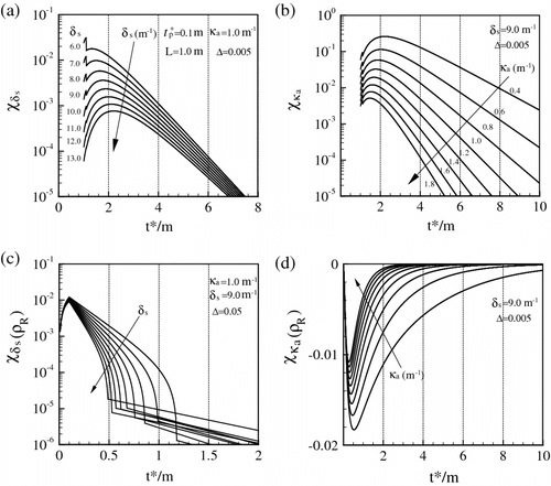
Figure 5 The sensitivity coefficients for and (i.e. and ) with respect to transmittance or reflectance signals ( and ) for different medium thicknesses (L) and pulse-width ()

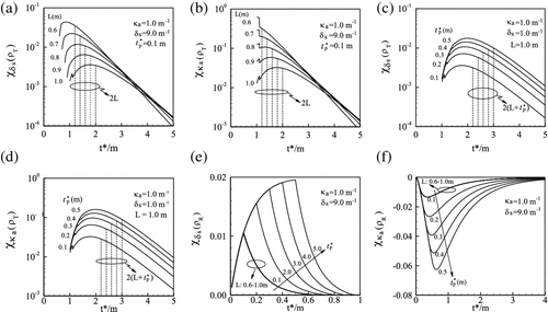
Firstly, Figure 5(a) and (b) shows the sensitivities and with respect to transmittance signal from thickness L = 0.6 to 1.0 m when the pulse width is 0.1 m. It can be seen that as the thickness L increased, the sensitivity coefficients and decreased and the location of the maximum and moved to right (the direction of increasing). However, the maximums of sensitivities are being included in the spans between start and 2L, no matter what L equals, from 0.6 to 1.0 m (see Figure 4(a) and (b)). Secondly, Figure 5(c) and (d) described that when the pulse width increase from 0.1 to 0.5 m (L is the constant of 1.0 m), the sensitivities of and with respect to rise and the maximum of and moved to right of the horizontal ordinate. In the same way, it can be found from Figure 5(c) and (d) that for every value of , the maximum sensitivities were contained during the interval of L- which was considered as the most sensitive spans of the transmittance signals for parameter estimation. At last, Figure 5(e) and (f) depict that and were not changed when the thickness L increase (). However, their absolute values ascended when the pulse width was changed from 0.1 to 0.5 m (L = 1.0 m). Both consider Figure 5(e) and (f) as the interval between 0 and that contains all the peak sensitivities for and with respect to the reflectance signals . In fact, is the length of the pulse laser that just completely transmits through the participating medium. After the above analysis, the span of [0, ] is very effective and sensitive for parameter estimation or inverse analysis.

4.2.2 Sensitivity coefficients with different optical properties (, or , )

In this section, in order to study whether all the sensitivity maximums are contained in the interval of [0, ], different optical properties were considered with the thickness L = 1.0 m and the pulse width . Then, is equal to 2.2 m.

Figure 6(a) and (b) depict the trend of and with respect to transmittance signals, when the scattering coefficients increase from 6.0 to 13.0 m⁻¹ and the absorption coefficients are not changed (). In Figure 6(a), as the coefficient increases (at the same time the albedo also increases), sensitivity decreases and its peak moves to the right. When increases to 10.0 (now is greater than 9.0), the length-dimensional time which corresponds to the maximum of (which is named as the peak location in the following text) has exceeded the interval (0, 2.2). On the contrary, when is less than or equal to 9.0, the peak location is still in the span of (0, 2.2). The similar conclusion could be obtained in the Figure 6(b). However, in Figure 6(c) and (d) the absolute maximums of and with respect to transmittance signals () have little change and all the peaks are in the span of (0, 2.2).

Figure 6 The sensitivity coefficients for and (i.e. and ) with respect to transmittance or reflectance signals ( and ) for different optical properties (, ).

In order investigate to the sensitive spans of radiative signals (especially transmittance signals) for the high-albedo media, the sensitivities for extinction coefficient with respect to and with high albedos ( = 0.90, 0.95 and 0.99) were studied. A tiny change in was set as 0.001% and the detailed results have been shown in Figure 7 and Table 2. It is apparent from Figure 7 that as the value of the extinction coefficient increases, all the sensitivity coefficients decreases; as the albedo increases, all the sensitivity coefficients also ascend. When the medium has a larger extinction coefficient, the transmittances are no longer sensitive and effective for optical parameter estimation. However, the reflectance signals are still sensitive and effective for optical parameter estimation. For example, when albedo is 0.90 and extinction coefficients are greater than 40 , the sensitivity coefficients are less than , while the maximums of sensitivity coefficients are larger more than 0.001. So, it could be concluded that reluctance signals are more sensitive and effective than transmittance signals in problems of estimation optical parameters for optically thick medium.

Figure 7 The sensitivity coefficients for (i.e. ) with respect to transmittance or reflectance signals ( and ) for different optical properties ( and ).

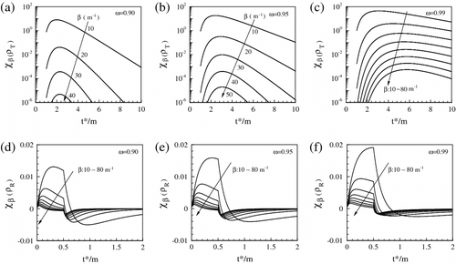
Table 2. The peak locations of sensitivity coefficients ( ), transmittance and reflectance signals ( )

	The peak locations ()	()
		10.0	20.0	30.0	40.0	50.0	60.0	70.0	80.0
0.90		1.99	2.26	2.31	2.31	N/A	N/A	N/A	N/A
		1.99	2.26	2.31	2.31	N/A	N/A	N/A	N/A
		0.31	0.16	0.11	0.08	0.06	0.05	0.04	0.04
		0.50	0.50	0.50	0.50	0.50	0.50	0.50	0.50
0.95		2.41	2.91	3.05	3.07	3.07	N/A	N/A	N/A
		2.41	2.91	3.05	3.07	3.07	N/A	N/A	N/A
		0.38	0.19	0.13	0.10	0.08	0.07	0.06	0.05
		0.50	0.50	0.50	0.50	0.50	0.50	0.50	0.50
0.99		3.11	4.46	5.13	5.49	5.67	5.75	5.78	5.78
		3.11	4.46	5.13	5.49	5.67	5.75	5.78	5.78
		0.50	0.26	0.18	0.13	0.11	0.09	0.08	0.07
		0.50	0.50	0.50	0.50	0.50	0.50	0.50	0.50

Table 2 describes the peak locations of sensitivity coefficients corresponding to transmittance and reflectance signals when increase from 10 to 80 , and are equal to 0.90, 0.95 and 0.99, respectively. As shown in Table 2, when and are greater than 0.9 and 10.0, respectively, all the peak locations for have exceeded the interval of (0, 2.2). As increases, the peak locations of increases to a constant value, while the peak locations of decrease. It is very noticeable that the peak locations of and transmittance signals are the same. In other words, the peak location of a transmittance signal is also the location where the sensitivity of with respect to this transmittance signal has its maximum. So, the spans which contain the peaks of the transmittance signals also contain the maximums of the sensitivity coefficients . Then, the peaks of transmittance signals could be used to determine the sensitive and effective sampling spans for parameter estimation. Furthermore, all the peak locations of the reflectance signals is 0.5 m and all the peak locations of is less than 0.5 m, which is less than 2.2 m, i.e. ).

In summary, after the sensitivity analysis for the optical properties (, or , ) with respect to radiative signals ( ), some criteria for choosing more sensitive spans of the measured signals used to estimate the optical parameters effectively can be obtained as follows:

1.	If the peak location of transmittance signal is less than , the span could be selected as [L, ].
2.	If the peak location of transmittance signal is more than , the selected span should contain the peak location. For example, the span could be (n = 3, 4, …). By the way, in this condition, the range of and could be determined ( and ).
3.	The effective span of reflectance signals could be selected as , which contain the peak locations of reflectance signals, as well as the maximums of all the sensitivity coefficients and .

4.3 The influences on the inverse results with different sampling spans

4.3.1 Case 1: 1-d uniform medium with different transmittance durations

In this case, 1-d uniform medium with black boundaries was considered. The length of the medium L is 1.0 m with the absorption coefficient and scattering coefficient as 1.0 m⁻¹ and 9.0 m⁻¹, respectively. The result of the transmittance signal obtained by forward model is shown in Figure 8. This result, with considering measurement errors of , was assumed as the time-resolved measurement transmittance data obtained by the surface detector. The size of searching space was set as [0, 20]. Only transmittance signal was used in the objective function. Three different sampling spans Case A–C are shown in Figure 8 and the fitness functions of three cases are shown in the Figure 11(a). Furthermore, the reconstructed results of the 300th generation for Case A–C and the relative errors are summarized in the Table 3. In addition, from Case A–C, the length dimensional time span is 2.2, 4.0 and 6.0 m, respectively. Because the time step is 0.01 m, for the inverse analysis of Case A–C, the number of points of the length dimensional time is 220, 400 and 600, respectively.

Figure 8 Case A–C with different sampling spans in Case 1.

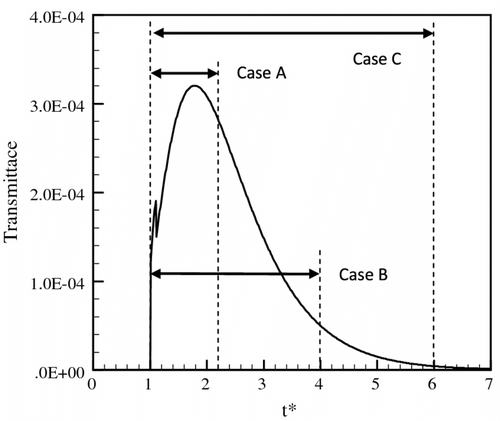
Figure 11 (a) The fitness functions of Case A–C in Case 1, and (b) the fitness functions of Case A–D in Case 2.

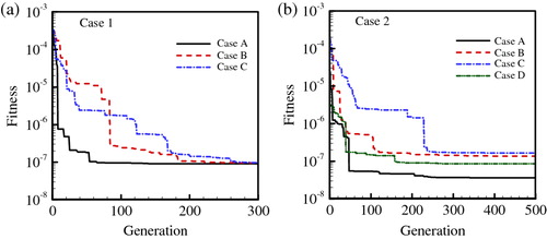
Table 3. The results of Case A–C with different sampling spans in Case 1 with noise

SPSO	Generation number	Time consuming (s)	Retrieval results or true value (m^−1)		Relative error (%)
			= 1.0	= 9.0
Case A	300	232	0.99631	9.02606	0.369	0.290
Case B	300	412	0.99736	9.01903	0.264	0.214
Case C	300	661	1.00111	8.98391	0.111	0.179

It is apparent from Table 3 that as the spans of the sampling time increases, the accuracy of the retrieved results increases, but the time-consuming of the inverse process also increases. The result of Case C is more accurate than Case B, which is more accurate than Case A. That is because the longer the sampling span, much more the information of the medium inside. However, the most time-saving span of sampling time is Case A, whose time consuming is approximately one-third of that of Case C. It also can be observed from Figure 11(a) that as the sampling span decreases, the fitness values descend more and more quickly. The fitness curve of Case A is the steepest curve in all three cases. However, all the three cases’ fitness reaches the magnitude of nearly at the generation 280 and after Generation 280, the three curves do not change any more. Furthermore, the results of Case A are retrieved correctly and the minimum relative error is not larger than 0.37%. Thus, Case A, which is the time span, should be selected as the optimum sampling span considering both time saving and accuracy.

As shown in Table 4, different absorption and scattering coefficients are estimated using the sampling span [L, ]. The pulse width is 1.0 m and the thicknesses of media are 1.0 and 0.6 m. So, the sampling spans are (1.0, 2.2) and (0.6, 1.4), respectively. The pairs of true parameters ( ) are (2.0, 8.0), (5.0, 5.0) and (8.0, 2.0), respectively, (which are satisfied with the Criterion I in section 4.2) and the measurement noise was set as 5%. The retrieved results listed in Table 4 are chosen when the generation number reached the 500th step in the SPSO process. It can be observed from Table 4 that all the relative errors are not more than 0.45%. So, the transmittance signals contained in the sampling span [L, ]could estimate the optical properties correctly and effectively.

Table 4. Estimation of different parameters using the sampling span [L, ] with noise .

L (m)	Sampling spans	True value of parameters ()		Inverse results ()		Relative errors (%)		Generation No.
1.0	(1.0, 2.2)	2.0	8.0	1.995	8.011	0.250	0.136	500
	(1.0, 2.2)	5.0	5.0	4.997	4.999	0.060	0.020	500
	(1.0, 2.2)	8.0	2.0	7.991	2.008	0.113	0.400	500
0.6	(0.6, 1.4)	2.0	8.0	1.993	8.033	0.350	0.413	500
	(0.6, 1.4)	5.0	5.0	4.999	4.995	0.020	0.100	500
	(0.6, 1.4)	8.0	2.0	7.965	2.009	0.438	0.450	500

4.3.2 Case2: 1-d two-layer medium with two reflectance peaks

In this case, the interface is regarded as transparent without reflected and refracted effects. In terms of the Lu and Hsu’s research [33], in 1-d two-layer medium, the reflectance with two peaks was occurred when the ratio of the laser pulse duration to the medium thickness L is less than 1.0 and the scattering coefficient of the forward layer is less than the backward layer (directed by the laser transfer direction). As shown in Figure 9, the medium was isotropic and optical parameters of the left layer were and . The under-layer properties , and the distance from the left wall to the interface will be estimated. Consider one step square pulse with the pulse duration incident the left wall of this medium. As shown in Figure 9, the reflectance results of the forward model with , and will be used as exact data to get the measurement data with the measurement error . The size of searching space was set as [0, 5]. Figure 10(a) describes four different spans of sampling time, noted Case A–D, are studied in this section. The sizes of sampling spans of these four cases, going from lowest to highest, are Case A, D, B and C, respectively. Figure 10(b) depicts the sensitivity coefficients , and with respect to the reflectance signal. It can be observed that Case B and C contain all the absolute maximums of these three sensitivity coefficients and all cases contain the absolute maximum of , while Case A and D do not contain the peak of .

Figure 9 The model that two-layer participating medium is irradiated by laser pulse in Case 2.

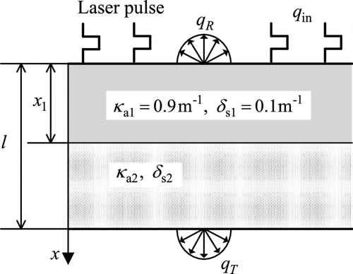
Figure 10 (a) Four different sampling spans of the reflectance signal for Case 2, and (b) sensitivity coefficients for , and with respect to the reflectance signal.

The retrieval of the absorption coefficient , scattering coefficient and distance on Generation 500 are listed in Table 5, which summarizes the true values and the retrieval values, as well as the relative error. As shown in Table 5, larger the sampling span, more time consuming the retrieval programme. Obviously, the retrieval results of and in Case B and Case C are all consistent with the true values. For Case B and Case C, the maximum for the three retrieved parameters ( and ) are not larger than 3.85% and 3.69%, respectively, with the measurement noise . Moreover, it can be seen from Table 5 that Case A failed to retrieve the optical property . In addition, Case D (0.1–1.7 m), with the sampling span being during the two peaks, failed to retrieve the absorption coefficient (with the absorption coefficient relative error being 25.09%). For Case A and Case D, the reason for unsuccessful parameters estimation may be due to the short sampling span of reflectance signals with not enough information of the medium inside. However, the distance was retrieved correctly in both Case A and Case D (relative error less than 1.47%) and it may conclude that the distance containing two reflectance signal peaks can be used to retrieve the positions of the layers in the two-layer medium. Furthermore, the fitness curves of Case A to D are shown in Figure 11(b), and it can be seen that shorter the sampling span is (A < D < B < C), more quickly the fitness curve descends, but more inaccuracy the results have (shown in Table 5). The fitness is calculated by Equation (26) and larger the sampling span is, more points of length-dimensional time are summed. So, the cases with larger spans may have a larger fitness; meanwhile, it has better accuracy estimation results and more time spending. In summary, both consider computational time and result accuracy synthetically. The sampling span of Case B would be selected as the best one in the four cases.

Table 5. The results of Case A–D with different sampling spans in Case 2 with noise .

SPSO ()		Case A	Case B	Case C	Case D
Sampling span (m)		(0–1.4)	(0–2.2)	(0–6.0)	(0.1–1.7)
Iteration number		500	500	500	500
Fitness value
Time consuming (s)		263	425	1141	320
True value or Retrieved results		0.06040	0.10385	0.10369	0.12509
		0.89431	0.9026	0.90129	0.90936
	x1 = 0.5 m	0.49269	0.49620	0.49795	0.49390
Relative error (%)		39.60	3.85	3.69	25.09
		0.63	0.29	0.14	1.04
	x1	1.462	0.76	0.41	1.22

Lu and Hsu [33] studied that when two peaks were occurred in the reflectance signal for the two-layer medium, the layer position could be obtained not using the complex inverse calculation, but the following formulation:(34) where and are the distance of the second layer form the laser-incident wall and the value of time with respect to the minimum value of the reflectance signals between the two peaks, respectively. And this conclusion can be validated in the present work.

In this section, considering both computational time and result accuracy synthetically in the inverse process, the better length-dimensional sampling span is 2.0 m obtained from Case B, which is just the two times larger than the medium length. In other words, the unknown parameters can be retrieved correctly using the span of the reflectance signals because there is enough useful information during this interval.

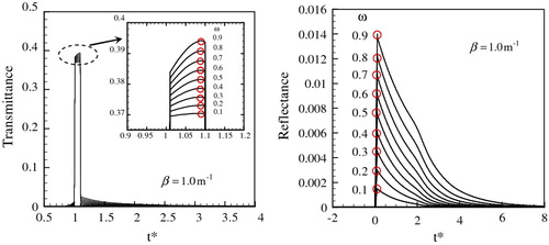
4.4 Inverse analysis only by means of the peak signal

In section 4.3, the sampling time which contains the peak of radiative signals could be used to estimate the optical properties and location of the interface correctly. In this section, only peak value of signals will be used to inverse the properties of uniform media. Consider the 1-d isotropic media, with thickness L of 1.0 m, extinction coefficient of 1.0 m⁻¹ and irradiated by one pulse with pulse width of 1.0 m. The true values of absorption and scattering coefficients for this homogeneous medium are and , respectively. The transmittance and reflectance signals with different albedo are shown in Figure 12(a) and (b), as well as the signal peaks indicated by dashed circles. It is apparent from Figure 12 that as the albedo of homogeneous media increases, the magnitude of the transmittance and reflectance also increase, as well as the peak values of these radiative signals. Because increasing albedos (i.e. increasing scattering coefficients) could cause more scattering heat flux leaving the boundary, it will increase the reflected or transmitted heat flux.

Figure 12 Peak values of transmittance signals (a) and reflectance signals (b) with different albedos in uniform media.

For the inverse problems, the peaks obtained by true values of and are used as measured data, while the peaks obtained by absorption and scattering coefficients changed from 0 to 2 , or 2 are considered as estimated data. The objective functions have been changed as follows:(35) where and are the peak values of the transmittance and reflectance signals, respectively.

Figure 13 described how objective function shapes change with the variation of absorption coefficients and scattering coefficients. It can be seen from Figure 13 that the objective function has a high sensitivity to the physical properties (absorption and scattering) of media, and Figure 13 illustrates the objective function shapes homogeneous media where only two parameters are to be recovered. For of 0.6–0.1, the 3-d shape of each objective function is in bowl shape, which allows a clear identification of the minimum. To the contrary, the flat shape () and valley shapes () are related to an ill-posed problem, which will retrieve parameters with larger errors. In summary, for the homogeneous medium with a small albedo, the objective functions close to a bowl with a well-defined minimum. Thus, absorption and scattering coefficients could be estimated accurately using radiative signal peaks for small-albedo homogeneous media.

Figure 13 Objective functions for two-parameter inverse problems using signal peak values.

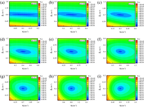
Shown in Figure 13, when the albedo is 0.9, the shape of objective function F(a) is a valley and the minimum magnitude of F(a) is 10⁻⁴. For , the true values of the scattering and absorption coefficients are 0.9 m⁻¹ and 0.1 m⁻¹, respectively. It can be seen from the picture that in the area with function fitness of , the scope of scattering coefficient is near 0.9 m⁻¹, while the range of absorption coefficients is from 0.08 m⁻¹ to 0.14 m⁻¹. In other words, the absorption coefficients have a larger fluctuation range than scattering coefficients in the area of . It indicated that the scattering coefficients could be estimated more accurately than absorption coefficients. That is because transmitted and reflected fluxes both mainly originate from light scattering; then, transmittance and reflectance signals contain more information about scattering coefficients than absorption coefficients. As the albedo decreases, the areas of decreases, as well as the fluctuation range of the absorption coefficients. When the albedo is equal or less than 0.5, the shape of the objective function F(a) is a bowl. It is apparent from Figure 13 () that absorption coefficients in areas do not fluctuate in a larger range, and now absorption and scattering coefficients could be estimated with high accuracy simultaneously.

With the noise of 1%, the inverse results of these cases using SPSO methods are shown in Table 6, which summarizes the albedo values, true values of coefficients, inverse data, as well as the relative errors. The size of searching space of the SPSO algorithm was set as [0, 5]. From these results, it is evident that the albedo change has a pronounced effect on the estimated accuracy of absorption value and the maximum relative error is 14%. However, the maximum relative error will be decreased to 7.1% when the iterative criterion is set as a smaller value of .

Table 6. The results of optical parameters estimated by radiative signal peaks with noise .

Albedo	True value		Inverse results		Relative errors		Iterative criterion
	Absorption (m^−1)	Scattering (m^−1)	(m^−1)	(m^−1)	(%)	(%)
0.9	0.1	0.9	0.1140	0.8963	14.0	0.41
0.9	0.1	0.9	0.10709	0.8966	7.09	0.37
0.8	0.2	0.8	0.1852	0.8036	7.40	0.45
0.7	0.3	0.7	0.2831	0.7041	5.63	0.59
0.6	0.4	0.6	0.4152	0.5997	3.80	0.05
0.5	0.5	0.5	0.5138	0.4973	2.76	0.54
0.4	0.6	0.4	0.5906	0.4008	1.57	0.20
0.3	0.7	0.3	0.7091	0.2985	1.30	0.50
0.2	0.8	0.2	0.8021	0.2006	1.05	0.30
0.1	0.9	0.1	0.9063	0.1004	0.70	0.40

Table 7 shows the estimation results with the noise of 5% and 10% when albedos are 0.1, 0.3, 0.5, 0.7 and 0.9, respectively. Apparently, for the same albedo , the relative errors are all larger than that of Table 6. From Table 7, when the albedo is 0.9, the relative errors for estimation of the absorption coefficients are 36.5% and 71.6%, while the relative errors for scattering estimation are 1.91% and 3.7% with the noises of 5% and 10%, respectively. When is 0.1, all the relative errors are smaller than 5%, especially to the results of the scattering coefficients; the errors are not more than 3.8%. Therefore, it can also be concluded that by using the peak values of radiative signals, estimate the scattering coefficient correctly even if the measurement noise reaches 10%. In addition, only the parameters of media with small albedo (such as, ) could be retrieved successfully. As for the media with big albedos, the absorption coefficients have not estimated correctly and larger the noise is, larger the relative errors are.

Table 7. The results of optical parameters estimated by radiative signal peaks ( = 5, 10%).

Measured noise	Albedo	True value		Inverse results		Relative errors		Iterative criterion
		Absorption (m^−1)	Scattering (m^−1)	(m^−1)	(m^−1)	(%)	(%)
	0.9	0.1	0.9	0.1365	0.8828	36.5	1.91
	0.7	0.3	0.7	0.3312	0.6880	10.4	1.71
	0.5	0.5	0.5	0.5287	0.4902	5.74	1.96
	0.3	0.7	0.3	0.7261	0.2941	3.73	1.97
	0.1	0.9	0.1	0.9219	0.0980	2.43	2.00
	0.9	0.1	0.9	0.1716	0.8667	71.6	3.70
	0.7	0.3	0.7	0.3651	0.6739	21.7	3.73
	0.5	0.5	0.5	0.5585	0.4813	11.70	3.74
	0.3	0.7	0.3	0.7518	0.2887	7.40	3.77
	0.1	0.9	0.1	0.9448	0.0962	4.98	3.80

5 Conclusion

In the present study, a finite-volume model has been developed and applied to simulate transient radiative transfer in the 1-d media. The analysis was done by considering the left boundary of the medium subjected to a short-pulse radiation due to the transient radiation process providing the valuable information for diagnostic and inverse analysis. The temporal profile of the pulse radiation was a step function. A squared medium with black boundary was studied to validate the FVM code.

Moreover, sensitivity analysis has been presented with different thickness, short pulse width and optical properties. The criteria for choosing more sensitive spans of the measured signals have been obtained. As to transmittance signals, if the peak location of the signal is less than , the sensitive span could be selected as [L, ]. When the peak location of the signal is larger than , the sensitive span could be selected as [L, ] (n = 2, 3, 4, …) which should contain the signal peak. As to reflectance signals, the effective span of reflectance signals could be selected as . After that, sampling spans of transmittance and reflectance signals were investigated. For the uniform media (Case 1), the best sampling span of the transmittance signals is the Case A with the interval of [1.0, 2.2] which is more efficient than others and it can get the correct retrieved results. In the two-layer media (Case 2), considering both computational time and result accuracy synthetically in the inverse process, the sampling span of Case B with the interval of [0, 2.2] should be selected as the better one.

At last, both transmittance and reflectance signal peak values for inverse analysis with different albedos were investigated. It is found that when only signal peaks were used as measured data to estimate the properties of uniform media, absorption coefficients were estimated more correctly than scattering coefficients, especially for big albedo cases. The scattering coefficients could be retrieved correctly for all the albedos with the maximum relative error not more than 0.6, 2.0 and 3.8% when the measurement noise are 1, 5 and 10%, respectively. In addition, the reconstruction of inhomogeneous media using radiative signal peaks will be studied in the future.

Table

Nomenclature
a	radiative parameter vector
c	the speed of light
c1, c2	the two positive acceleration coefficients in Equation (18)
F	objective function of minimization
H	Heaviside step function
I	radiation intensity,
L	length of the media, m
l	the pulse propagating distance from incident location in direction
M	number of particles in each swarm
n	the dimension of the problem or the present time step
n − 1	the previous time step
	number of polar angle
	number of azimuthal angle
	the global best position discovered by all particles at generation t
	the local best position of particle i discovered at generation t or earlier
	heat flux
	heat flux of collimated incident light at boundary ,
	reflected heat flux
	transmitted heat flux
	uniform random number in [0, 1]
S	the radiative source term
t	time or generation in SPSO algorithm
tp	pulse laser duration (the width of pulse)
	the start time of sampling span
	the end time of sampling span
	span of sampling time
	length-dimension time step
U	the retrieval variable
	velocity array of ith particle in PSO
	the velocity of the ith particle with jth dimension at generation t
Vmax	the maximum velocity
w	the inertia weight coefficient
	the minimum value of the search space
	the maximum value of the search space
	the position array of the ith particle in PSO
	the position of the ith particle with jth dimension at generation t
Y	measured or exact parameter
Greeks symbols
	the factor of time difference schemes,
	extinction coefficient, ()
	Dirac delta function
	scattering coefficient,
	a small specified positive number or emissivity
	scattering phase function
	measured errors,%
	absorption coefficient,
	direction cosine
	time-resolved transmittance or reflectance
	standard deviation
	a normal distributed random variable
	optical thickness
	sensitivity coefficient
	single scattering albedos ()
	solid angle, sr
	scattering direction or outgoing direction
	incoming direction
	unit vector in the incident radiation direction
Subscripts
b	blackbody
c	collimated radiation component of incident laser pulse
d	diffused radiation component of incident laser pulse
est	estimated value
in	incident laser pulse
	iteration number
L2	L2-type norm
mea	measured value
min	minimum value
max	maximum value
p	laser pulse
R	reflectance
T	transmittance
w	boundary wall
Superscripts
m	the mth discrete solid angle
T	matrix transpose
	the length dimension or dimensionless term

Acknowledgement

The support of this work by the National Natural Science Foundation of China [No. 51,076,037], the Foundation for Innovative Research Groups of the National Natural Science Foundation of China [No. 51,121,004] and the Fundamental Research Funds for the Central Universities [No. HIT. BRET 1. 2,010,012] are gratefully acknowledged.

References

- André Charette, A, Joan Boulanger, B, and Kim, HK, 2008. An overview on recent radiation transport algorithm development for optical tomography imaging, JQSRT 108 (2008), pp. 2743–2766.
- Dolin, LS, Shchegol’kov, YB, and Shchegol’kov, DY, 2008. Experimental verification and refinement of the model of light-beam brightness fluctuations in a turbid medium with randomly nonuniform absorption, Radiophys. Quantum Electron. 51 (2008), pp. 222–237.
- Schmitt, JM, and Kumar, G, 1996. Turbulent nature of refractive-index variations in biological tissue, Opt. Lett. 21 (1996), pp. 1310–1312.
- Kravtsov, YA, and Apresyan, LA, 1996. Radiative transfer: new aspects of the old theory, Prog. Opt. 36 (1996), pp. 179–244.
- Beuthan, J, Minet, O, Helfmann, J, Herrig, M, and Müller, G, 1996. The spatial variation of the refractive index in biological cells, Phys. Med. Biol. 41 (1996), pp. 369–382.
- Berg, R, Jarlman, O, and Svanberg, S, 1993. Medical transillumination imaging using short-pulse diode lasers, Appl. Opt. 32 (1993), pp. 574–579.
- Han, W, Eichholz, JA, Huang, J, and Jia, L, 2011. RTE-based bioluminescence tomography: a theoretical study, Inverse Prob. Sci. Eng. 19 (2011), pp. 435–459.
- Han, W, Cong, WX, and Wang, G, 2006. Mathematical theory and numerical analysis of bioluminescence tomography, Inverse Prob. 22 (2006), pp. 1659–1675.
- Klose, AD, and Hielscher, AH, 1999. Iterative reconstruction scheme for optical tomography based on the equation of radiative transfer, Med. Phys. 26 (1999), pp. 1968–1707.
- Arridge, SR, Dehghani, H, Schweiger, M, and Okada, E, 2000. The finite element model for the propagation of light in scattering media: a direct method for domains with nonscattering regions, Med. Phys. 27 (2000), pp. 252–265.
- Ripoll, J, Nieto-Vesperinas, M, Arridge, SR, and Dehghani, H, 2000. Boundary conditions for light propagation in diffusive media with nonscattering regions, J. Opt. Soc. Am. A. 17 (2000), pp. 1671–1682.
- Trivedi, DA, Mitra, K, and Vo-Dinho, T, 2003. Experimental and numerical analysis of short-pulse laser interaction with tissue phantoms containing inhomogeneities, Appl. Opt. 42 (2003), pp. 5173–5180.
- Mishra, SC, Chug, P, Kumar, P, and Mitra, K, 2006. Development and comparison of the DTM, the DOM and the FVM formulations for the short-pulse laser transport through a participating medium, Int. J. Heat Mass Transfer. 49 (2006), pp. 1820–1832.
- Chai, JC, 2003. One-dimensional transient radiation heat transfer modeling using a finite-volume method, Numer. Heat Transfer, Part B. 44 (2003), pp. 187–208.
- Sakami, M, Mitra, K, and Hsu, PF, 2002. Analysis of light-pulse transport through two-dimensional scattering and absorbing media, JQSRT. 73 (2002), pp. 169–179.
- Muthukumaran, R, and Mishra, SC, 2008. Thermal signatures of a localized inhomogeneity in a 2-D participating medium subjected to an ultra-fast step-pulse laser wave, JQSRT. 109 (2008), pp. 705–726.
- Guo, Z, and Kumar, S, 2002. Three-dimensional discrete ordinates method in transient radiative transfer, AIAA. J. Theomorphic Heat Transfer. 16 (2002), pp. 289–296.
- Chai, JC, Hsu, PF, and Lam, YC, 2004. Three-dimensional transient radiative transfer modeling using the finite volume method, JQSRT. 86 (2004), pp. 299–313.
- Kennedy J, Eberhart RC. Particle swarm optimization. Proc. IEEE Int’1. Conf. on Neural Networks, IV. Piscataway, NJ; 1995..
- Cui ZH, Zeng JC, Cai X. A new stochastic particle swarm optimizer. Proceedings of the 2004 congress on, evolutionary computation (CEC). 2004;1:316–319..
- Cui, ZH, and Zeng, JC, 2004. A guaranteed global convergence particle swarm optimizer, lecture notes in artificial intelligence, Vol. 3066. Sweden: Springer; 2004, p. 762–767.
- Al-kazemi B. Multi-phase Particle Swarm Optimization [PhD thesis]. USA: Syracuse University; 2002..
- B. Al-kazemi, and C. K. Mohan, Discrete Multi-Phase Particle Swarm Optimization. Information Processing with Evolutionary Algorithms: From Industrial Applications to Academic Speculations; (2005), p. 305-327..
- Lee, KH, Baek, SW, and Kim, KW, 2008. Inverse radiation analysis using repulsive particle swarm optimization algorithm, Int. J. of Heat Mass Transfer. 51 (2008), pp. 2772–2783.
- Lee, KH, Baek, SW, Kim, KW, and Kim, MY, 2007. A study on inverse radiation analysis using RPSO algorithm, Trans. Korean Soc. Mech. Eng. 31 (2007), pp. 635–643.
- Coello Coello, CA, Pulido, GT, and Lechuga, MS, 2004. Handling multiple objectives with particle swarm optimaization, IEEE Trans. Evol. Comput. 8 (2004), pp. 256–279.
- Qi, H, Wang, DL, Wang, SG, and Ruan, LM, 2011. Inverse transient radiation analysis in one-dimensional non-homogeneous participating slabs by using particle swarm optimizer algorithms, J. Quant. Spectrosc. Radiat. Transfer 112 (2011), pp. 2507–2519.
- Modest, MF, 2003. Radiative heat transfer. New York, NY: Academic Press; 2003.
- Balima, O, Charette, A, and Marceau, D, 2010. Comparison of light transport models based on finite element and the discrete ordinates methods in view of optical tomography applications, J. Comput. Appl. Math. 234 (2010), pp. 2259–2271.
- An W. finite element method for radiative transfer and research of time-resolved inverse radiation problem [Dissertation for the Doctoral Degree in Engineering].Harbin: Harbin Institute of Technology; 2007..
- An, W, Ruan, LM, Tan, HP, and Qi, H, 2007. finite element simulation for short pulse light radiative transfer in homogeneous and non-homogeneous media, ASME J. Heat Transfer. 129 (2007), pp. 352–362.
- Ruan, LM, An, W, Tan, HP, and Qi, H, 2007. Least-squares finite element method for multidimensional radiative heat transfer, Numer. Heat Transfer, Part A 51 (2007), pp. 657–677.
- Lu, XD, and Hsu, PF, 2005. Reverse monte carlo simulations of light pulse propagation in non-homogeneous media, J. Quant. Spectrosc. Radiat. Transfer. 19 (2005), pp. 353–359.