The concept of distance in global optimization applied to non-linear inverse problems

Abstract

A common approach to solve an inverse problem, i.e. to single out the model parameters that explain the observed phenomena, is to iteratively minimize a residual function, which expresses the difference between the observations (measured data) and the forward response of the estimated model (recalculated data). The convergence properties of the solver can be difficult to control and to analyse, especially when dealing with global optimizers applied to non-linear inverse problems. In this paper, we plot the residual vs. a single scalar, the Euclidian distance in the variable space. We show how this can be used to avoid misleading solutions given by the local minima. The performance of this approach is investigated in three examples with increasing complexity (in terms of dimensions). Moreover, we propose to exploit the distance indicator in a new hybrid inversion strategy that combines a simulated annealing algorithm and a local approach and that reduces the computational cost of the optimization.

Keywords:

• global optimization
• simulated annealing
• convergence
• local search

AMS Codes:

• 49N45
• 65B99

View correction statement:

Corrigendum

1. Introduction

A common approach to solve an inverse problem, i.e. to single out the model parameters (variable space) that explain an observed phenomena, is to iteratively minimize a residual function, which expresses the sum of the squared difference (L² norm) between the observations (measured data) and the forward response of the estimated model (recalculated data).[1]

As in a wide variety of physical problems, the law linking the model to the data is non-linear and multimodal, the solution requires techniques based on systematic search. This explores the variable space, it computes the residual for each explored point and it finds the model corresponding to the minimal data residual.

For this class of inverse problems, the retrieval may results in unsatisfactory solutions, as local search for the least squares solution is likely to get trapped in secondary minima. A global search can avoid sub optimal solutions, but it is time and computation consuming [2] due to convergence issues.[3–8] In problems with a small number of dimensions (⩽three), either an exhaustive search or the visualization of the problem solution overcomes these difficulties.

These considerations suggested to the authors the idea of combining the advantages of a global optimizer with the efficient convergence of a local search engine. To do so, the authors resort to a criterion that ensures that the switch from the global approach to the local one takes place unambiguously, i.e. in the region where the solution is unique.

With high dimensional optimization problems, it is not practical to plot the residuals. But collapsing the variable space to one dimension makes the displaying of the residuals easy. Among other choices, this can be performed using the Euclidian distance between a reference point and each point in the variable space. Collapsing an nD quantity to a 1D one introduces ambiguities and distortions. In this perspective, Euclidian distance benefits of the L²-norm propriety of emphasizing the weight of both little and great errors better than any L¹-norm criterion.

The inversion works as follows: the global optimizer stops its function calls as soon as it reaches the 1D interval containing a unique minimum. Then, a local search refines the solution. In this framework, one can choose whichever global and local optimizer either according to the specific problem or to its availability.

The global optimizer applied in this work is based on the simulated annealing technique as it intrinsically takes into account the available information about the physical system, such as the bounds of some model parameters or a rough estimate of their values.[9]

Analysing the global optimization behaviour of the simulated annealing algorithm, it can be observed that a significant part of the computational effort is spent in the final steps of the optimizing procedure, when the region containing the best local optimum has already been identified.[10,11] This reveals that it is attractive to stop the algorithm before of its standard procedure of termination, activating a local search technique to find the best local optimum. In this work, the employed local search engine is a standard iterative gradient method. The original implementation of the simulated annealing [9] was re-formulated to include the stop criterion that triggers the switch between the global and the local approach.

The performance of this approach is investigated in three examples with increasing complexity. These were chosen in order to focus on some of the aspects that could affect the quality of the retrieved solution.

The first example is related to the alignment of time series, which has its interest in a range of application involving stochastic processes and data mining. This example highlights the misleading effect of local minima and it is useful to discuss possible countermeasures. The second example pertains to the Atmospheric Sciences and it consists of the retrieval of the two-dimensional structure of the atmospheric specific absorption coefficient from the observations of a ground-based scanning radiometer. The third example considers a homogenous 1D seismic inversion aiming to retrieve the acoustic impedances I_P. Here, we discuss the re-parameterization of the variable space. The original concept of Drufuca and Rovetta was formalized and implemented by Rovetta in his master thesis [12] and later included in his PhD thesis.[13]

The paper is organized as follows. Section 2 describes the distance indicator together with its properties. Section 3–5 reports the benefits of the proposed approach to the solution of the inverse problem for the three chosen examples. Conclusions are drawn in Section 6. Details about the hybrid simulated annealing implementation are given in Appendix 1.

2 The distance indicator

Let us assume that the forward problem is described by the vectorial non-linear function $\mathit{y}=g(\mathit{m})$ and that the dimension of the vector y (data space), and the dimension of the vector m, (variable space), are equal to N and M, respectively.

The inversion scheme aims to identify the vector m for which an objective function $f(\mathit{m})$ is minimized. It is evaluated as the square of the amplitude of the residual:(1) $f(\mathit{m})=(\mathit{y}-g(\mathit{m}){)}^T(\mathit{y}-g(\mathit{m}))=\sum _{i=1}^N(y_i-g_i(\mathit{m}){)}^2$(1)

where the apex T stands for the transpose. A mono-dimensional representation of this function can be achieved by using the concept of Euclidian distance, whose square is equal to:(2) $d^2=(\mathit{m}-{\mathit{m}}_{\text{ref}}{)}^T(\mathit{m}-{\mathit{m}}_{\text{ref}})=\sum _{j=1}^M(m_j-m_{\text{ref,}j}{)}^2$(2)

with m_ref a reference value for m. The choice of the reference depends on the specific problem. It could be an estimate from a previous forward solution or a first guess from known physical properties of the application under study. At each function call in the simulated annealing, the objective function and the distance d are computed.

The distance d has the purpose of collapsing the dimensions of the variable space to one only. This facilitates the monitoring of the evolution of the objective through the iterations. In the initial stages, more than one attractive basin will be observable while, near convergence, there will be only one. Near convergence one can avoid the lengthy process of simulated annealing, as one can resort to a more efficient local search engine, for instance, a gradient approach. Essentially, the stopping criterion is based on a heuristically set parameter that the authors named sensitivity on the convergence criterion. This parameter governs the switch between the two approaches according to the minimum acceptable value of the distance error standard deviation. Details about the stopping criterion are given in Appendix 1, where the advantages of the hybrid strategies are reported.

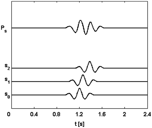
To underline the potentiality of this approach, let us consider a simple two-dimensional problem of aligning in the time domain two signals (M = 2), s₁ and s₂, with respect to a reference one, s₀ (Figure 1).

Figure 1 2D example without noise; starting point: low energy stack of the two not aligned signals s₁ and s₂ with respect to the reference one s₀.

The data residual can be defined as:(3) $f(\mathit{\tau })={\left[\sum _{i=1}^N(2s_{0\text{,}i}-s_{1\text{,}i}({\tau }_1)-s_{2\text{,}i}({\tau }_2){)}^2\right]}^{\frac{1}{2}}={\left[\sum _{i=1}^N{\left(2s_{0\text{,}i}-\sum _{j=1}^2{s}_{j\text{,}i}({\tau }_j)\right)}^2\right]}^{\frac{1}{2}}$(3)

where m = τ is the vector of the model parameters and it collects the time delay of the signals s₁ and s₂, with respect to s₀, while y = 2s₀ is the vector of the data space. $g_i(\mathit{m})={\sum }_{j=1}^2{s}_{j\text{,}i}(m_j)$ is the ith component of $g(\mathit{m})$. The distance is computed in the time delay domain by choosing as reference the delay τ₀ = 0 of the signal s₀.

It can be proved [14] that the minimization of the cost function $f(\mathit{\tau })$ corresponds to the maximization of the stack power $P_{\text{S}}=\frac{1}{N}{\sum }_{i=1}^N{\left[{\sum }_{j=0}^2{s}_{j\text{,}i}({\tau }_j)\right]}^2\text{,}$ (sum of the signals), with τ₀= 0. P_S is shown in Figure 2, as a function of both τ₁ and τ₂, after normalization.

Figure 2 Normalized stack power P_S of the signals s_i; i = 0, … , 2, as a function of the delay times ${\tau }_1$ and ${\tau }_2$. The pick corresponding to the global maximum is marked with a white circle.

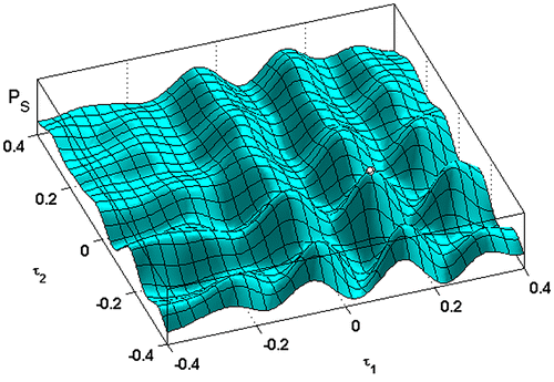
Figure 3 shows the stack power P_S computed for all the investigated points vs. the distance d = $\sqrt{{\tau }_1^2+{\tau }_2^2}$. The domain of local stationariness and the global maximum of the stack power function are well detected. It is useful to underline that the sampling is uniform in the domain of the time delays, but not in the domain of the distance.

Figure 3 Normalized stack power P_S of the signals s_i; i = 0, … , 2, as a function of the distance. The domain of local stationariness and the global maximum are well detected.

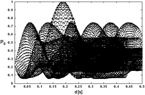
Because of the high multimodality of the objective function, the maximization of the stack power can be achieved by a global optimization algorithm based on a controlled exploration of the domain of the time delays.

A simulated annealing algorithm, referred to as SAA in the following, helps us in tracking the evolution of the maximization process, according to the changing values of the control parameter T_A, known as the annealing temperature.[9] The behaviour of the algorithm from the starting point to the convergence is shown in Figure 4(a). Some evaluations of the stack power at different annealing temperatures are represented in Figure 4(b) and (c). At high temperatures, the algorithm works as a common uniform sampler, while at low temperatures, the sampling interval is located in the model domain corresponding to the highest posterior probability density of the global maximum.

Figure 4 Normalized stack power P_S: path of the SAA from the starting solution to the final one; evaluations of the objective function at different annealing temperatures: starting temperature, T₀ = 300 (a), intermediate temperature, T_A = 23 (b) and final one T_f = 14 (c).

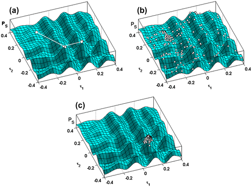
The visual representation of the data residual is possible in this example because of the dimension of the model space. When the model dimensions are greater than three, a way to give a visual representation of the data residual is through the distance of the model space that singles out the properties of local stationariness, as it is shown in the following sections.

3 Optimal signal alignment

In this section, the performance of the distance indicator is validated against a generalization of the previous example by increasing the number of signals to align. Let us consider M signals s_i (i = 1, … , M), with a delay time τ_i with respect to a reference signal s₀.

If the number of samples for each signal is equal to N, then the stack power can be valued as:(4) $P_{\text{s}}=\frac{1}{N}\sum _{i=1}^N{\left[\sum _{j=0}^M{s}_{j\text{,}i}({\tau }_j)\right]}^2$(4)

with τ₀ = 0.

The optimal alignment, obtained maximizing P_S, is the result of a multidimensional non-linear optimization problem and again its solution was achieved by means of SAA.

The data-set discussed in this example is a noisy one (SNR = 4 dB with uniform noise in the signal bandwidth) with N = 600 and M = 20. Following the standard SAA approach, the starting and the final temperatures of the algorithm are $T_0=300$ and $T_{\text{f}}=117$, respectively. According to (A1), the total number of evaluations of the objective function is equal to $N_{\text{F}}=9.6\times {10}^5$, being N_S = 20 and N_T= 100.

Figures56 show the raw and the aligned data, respectively, whereas Figure 7(a) and (c) illustrate the normalized stack power P_S vs. the distance at different annealing temperatures.

Figure 5 Example with noise and model space of 20 dimensions; starting point: not aligned signals s_i; i = 1, … , 20 and stack with low energy.

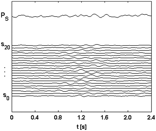
Figure 6 Example with noise and model space of 20 dimensions; final solution: optimal signal alignment and stack with maximum energy.

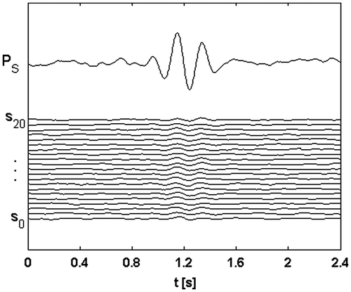
Figure 7 Example with noise and variable space of 20 dimensions. Distances at different annealing temperatures: starting temperature T₀ = 300 (a); T_A = 156, corresponding to the sixteenth change of temperature; two local maxima can be detected (b); final temperature, T_f = 117; the global maximum has been found (c).

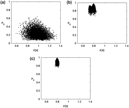
When the annealing temperature T_A of the algorithm is high it is not possible to detect the domains of stationariness of the objective function (Figure 7(a)). These latter become observable only when T_A reduces significantly (Figure 7(b)), and at convergence, after 24 changes of the annealing temperature, the algorithm identifies the best one among all of the local maxima (Figure 7(c)).

By using the distance indicator, the region containing the global maximum is detected at the 16th iteration. The number of function evaluation reduces of 1/3. At this point the solution is refined with a gradient method.

4 The retrieval of two-dimensional absorption coefficient structure from a scanning radiometer

This second example shows the retrieval of the 2D structure of the atmospheric specific absorption coefficient through a tomographic acquisition of the brightness temperature values. These are collected at the frequency of 23.8 GHz by using a ground-based radiometer located at Spino d’Adda, 30 km SE of Milan (Italy). Here, we recall the basic considerations and we show a result obtained through global optimization, while the reader is referred to [15] for the details of the experiment and the modelling. The central idea is to infer the status of the atmosphere, i.e. the integrated water vapour content, by means of the values of the measured brightness temperature.[16] The problem is intrinsically ill-posed because of many factors among which there are the predominant vertical trend with respect to the horizontal one [17] and the limited number of tomographic projections.[18]

The algorithm performs the inversion of the non-linear function that describes the forward problem, linking the absorption coefficients to the brightness temperatures radiative transfer equation.[16]

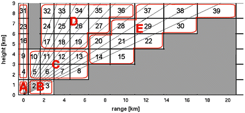
The scanned vertical plan is divided into M bins as shown in Figure 8. Each bin gives a contribution to the measured brightness temperature T_Bi in the direction θ_i through the following scheme:(5) $T_{\text{Bi}}=\sum _{i=1}^M{k}_j{T}_j\times (1-{\tau }_{\mathit{ij}})\mathrm{\Delta }{r}_{\mathit{ij}}=\sum _{j=1}^M{k}_j{T}_j\left(1-\sum _{l=1}^{j-1}{k}_l\mathrm{\Delta }{r}_{\mathit{il}}\right)\mathrm{\Delta }{r}_{\mathit{ij}}$(5)

Figure 8 The scanned vertical plan is divided in resolution bins – black boxes – with constant atmospheric specific absorption coefficient. Maximum altitude is fixed at 9 km and range at 23 km, according to the elevation of the lowest scan. Solid lines represent the propagation path seen by the radiometer antenna. Since the problem is ill-conditioned, a re-parameterization led to collapse the 39 bins into 5 macrocells – depicted in red – according to a clustering strategy.

where ${\tau }_{\mathit{ij}}={\sum }_{l=1}^{j-1}{k}_j\mathrm{\Delta }{r}_{\mathit{il}}$. T_j and k_j are the physical temperature and the specific absorption coefficient in the jth bin, Δr_ij is the length of the ray corresponding to the ith angle and the jth bin ($\mathrm{\Delta }{r}_{\mathit{ij}}$ = 0 if the ray does not cross the bin). ${\tau }_{\mathit{ij}}$ is the optical thickness linking the jth bin to the receiver through the ith elevation angle. In Equation (5), the contribution from T_C has been neglected [15] and the integrated water content is accounted for through its specific absorption coefficient.

The data-set is composed of 12 brightness temperature values observed along paths with different elevation angle with respect to the local horizon, as depicted in Figure 9.

Figure 9 Observed brightness temperatures (circles) vs. the co-elevation angle.

After re-parameterization, through a clustering strategy, the cardinality of the model space is reduced to M = 5 (see Figure 8).

We find an approximate solution through:(6) $\text{min}\left(|{\mathit{T}}_{\mathbf{B}}-f(\mathit{K}){|}^2\right)$(6)

in which f(K) is the matricial formulation of the forward problem as it appears in Equation (5). T_B and K are the vector in the data and in the variable space, respectively.

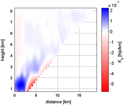
The observations and the recalculated data from the estimated model are computed as variation with respect to a common reference – chosen as the vertical trend of the standard atmosphere [19] – and then compared in Figure 10. The recalculated data are close to the observed data (R_d= 0.5). Figure 11 shows the solution of the inverse problem, which is the 2D structure of the atmospheric specific absorption coefficient after vertical detrending and interpolated with a kriging technique.

Figure 10 Observations (circles) and recalculated data (asterisks) as variation with respect to the vertical trend of the standard atmosphere.

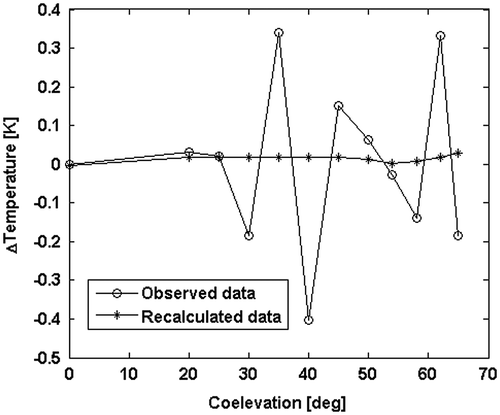
Figure 11 Estimate of the two dimensional specific absorption coefficient k of the atmosphere after vertical detrending: the solution is interpolated with a kriging technique.

The starting and the final temperatures of the standard SAA are equal to T₀ = 100, T_f = 0.9 and the number of the total evaluations of the objective function is $N_{\text{F}}=2.36\times {10}^6$, being N_S= 20 and N_T= 195 (A1). The hybrid SAA requires 37 annealing temperature reductions, instead of 121, thus resulting in a computational cost reduction of about 69%.

During its execution, it can happen that SAA evaluates the objective function in points of the variable space that lay outside of the observation domain, whose bounds are given. In such a situation, the algorithm rejects the point and it chooses a different one inside the observation domain with a random selection.

At high temperatures, the explored domain is quite large because of both the long exploration steps of the algorithm and the occurrence of the bound events. There is not any attraction domain and the data residuals are quite high (Figure 12(a)).

Figure 12 Data residual as a function of the distance at different annealing temperatures: T₀ = 100 (a); T_A = 72 (b); T_f = 0.9 (c).

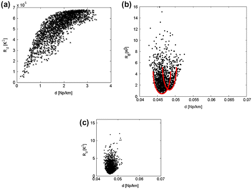
When the model parameters approach the convergence, the local minima with the lowest data residual can be easily identified (Figure 12(b)). At the convergence, when all the estimated parameters are close to the minimum, chosen as the solution of the inverse problem, the shape of the domain corresponding to the global optimum is shown and the data residuals are all low (Figure 12(c)). In this case, plots of the data residual vs. the distance permit to verify the presence of the global minimum.

5 1D homogeneous seismic inversion

The last application concerns the seismic experiment where elastic waves produced by explosions or vibrating controlled sources are propagated through the Earth and recorded at or near the surface in order to map the underground geology. Specifically, we focus on the seismic inversion problem whose objective is to infer from the seismograms (observed data), acquired by an array of receivers lying on the ground, the underlying earth structure (model parameters).[20,21]

To simplify the problem, a layered model of the Earth is used: the rock densities ρ and the elastic wave velocities v vary with the depth z only. Moreover, the seismic experiment is conducted with one source and one receiver, located at the same position on the surface (zero-offset measurement). Data collected with this set-up only contain information on the travel time between the layer’s interfaces and on the contrast in acoustic impedances at these interfaces. Therefore, without imposing additional constraints, the unknown quantities that can be estimated are the acoustic impedances I_P (the product of the rock densities with the velocities v_P of the P-waves).[22,23]

Nonetheless, to discuss the parameterization of the model space by using the distance indicator, the problem is first inverted for a model vector m, made up of the rock densities ρ and from the P-wave velocities v_P of the 20 micro-layers (the dimensions of the variable space are M = 40).

The observations are generated from a synthetic model, by using an algorithm based on the well-known reflectivity method .[24] They are shown in Figure 13.

Figure 13 Observed data. n_S denote the number of samples of the seismogram.

The solution of the forward problem used by SAA in the inversion process is a coarse approximation: the interface scatter coefficients are calculated by means of the transmission line theory [25,26] and the seismograms by the convolution theory. The differences in the algorithms used to compute the observed synthetic data (reflectivity method) and the data recalculated by the estimated model (transmission line theory and convolution theory), imply a modelling noise corresponding to an SNR on the seismograms of about 23 dB.

The number of the layers of the posterior model is unknown and for this reason it is necessary to use an over-parameterized a priori model. To simplify the problem, a synthetic model with 10 layers is used to compute the data, while the a priori model with 20 micro-layers is employed in the inversion.

The mapping of the data residual R_d on the domain of the distance d is discussed varying the annealing temperature T_A from T₀= 10⁻³ to T_f = 7 × 10⁻¹². At the highest temperatures, the analysed domain is quite large due to the long exploration steps of the algorithm. Also, there are not evident attraction domains and all the residual data are high (Figure 14(a)).

Figure 14 Inversion for v_P and ρ. Data residual as a function of the distance at different annealing temperatures: T₀ = 10⁻³ (a); T_A = 2 × 10⁻⁹ (b); T_f = 7 × 10⁻¹² (c). The white mark corresponds to the optimal solution at each annealing temperature.

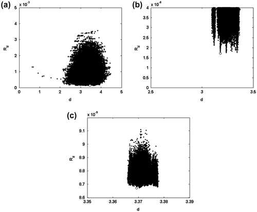
At lower temperatures, the domains of attraction can be observed and some local minima with lower data residual can be detected (Figure 14(b)). Finally, at the convergence, all the model parameters are close to the minimum chosen like the model domain of the solution (Figure 14(c)).

The optimizing algorithm evaluates the objective function 14 million of times. This corresponds to 1/5th of the number of evaluations required by the standard SAA algorithm.

A correct inversion of such a model vector (rock densities and P-wave velocities) is not possible because of the high condition number of the inverse problem: this is shown by the presence of a number of minima with the same data residual. Therefore, the solution (i.e. one of these minima) is not reliable and a re-parameterization of the model space is mandatory. Then, the problem is inverted for a model vector m, composed of the acoustic impedances I_P of the 20 micro-layers (the variable space dimensions reduce to M = 20).

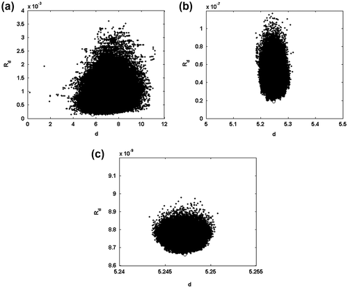
Let us consider again the data residual R_d(d): at high temperatures (Figure 15(a)), the behaviour is similar to the one shown in the previous inversion, but at lower temperatures, there are not many local minima with the same data residual, the objective function is convex and the solution is reliable (Figures 15(b) and (c)).

Figure 15 Inversion for I_P. Data residual as a function of the distance at different annealing temperatures: T₀ = 10⁻³ (a); T_A = 2 × 10⁻⁹ (b); T_f = 7 × 10⁻¹² (c). The white mark corresponds to the optimal solution at each annealing temperature.

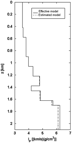
The estimated and the effective models are compared in Figure 16. The matching is optimal but in the last layer, which cannot be solved because it is low unbounded.

Figure 16 Acoustic impedances I_P vs. the depth z; comparison between the effective model (solid line) and the estimated model (dashed line).

It is interesting to underline that in the previous example the global minimum (white circle marker in Figure 15(c)) can be detected at the 66th iteration on the total number of 84: again, the SAA is stopped before it normally completes its execution and the solution is retrieved with a local technique (gradient algorithm), in order to reduce the computational cost (see Appendix 1).

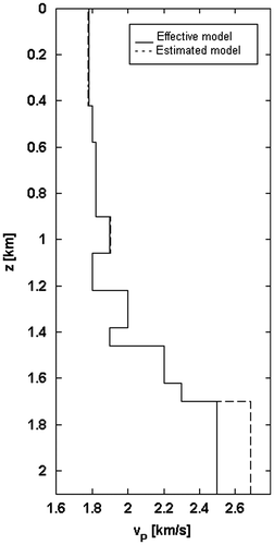
Once the acoustic impedances I_P are estimated, it is also possible to recover the rock densities ρ and the P-wave velocities v_P by introducing a modelling constraint, i.e. that every impedance contrast corresponds to an interface between layers. The values of ρ and v_P, obtained under this assumption, are compared with the actual model and shown in Figures1718.

Figure 17 Rock densities ρ vs. the depth z; comparison between the effective model (solid line) and the estimated model (dashed line).

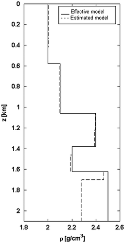
Figure 18 P-wave velocities v_P vs. the depth z; comparison between the effective model (solid line) and the estimated model (dashed line).

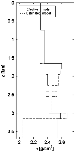
We generalized the problem to the case of a seismic inversion with many receivers at different offsets from the source location. This acquisition scheme permits to retrieve both elastic impedances I_P and I_S. In the post-processing phase, by introducing the same modelling constraint of the zero-offset problem, it is possible to estimate the rock densities, the P-wave and S-wave velocities.

The forward model employed in the inversion algorithm requires a ray tracer. The differences between data computed with this algorithm and those obtained with the reflectivity method (employed to generate the observed synthetic data) lead to a modelling noise corresponding to an SNR on the seismograms of about 26 dB. The inversion procedure is practically the same of the zero-offset case.

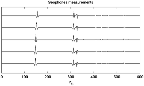
In the following, we show an example based on the measurements from five geophones and one a priori model of 20 micro-layers (the cardinality of the model is equal to M = 40).

The observed data are shown in Figure 19, while the results of the inversion are depicted in Figures 2021222324. The estimated elastic impedances and velocities fit their actual values with a good accuracy, except for the last layer, as pointed in the previous example. The additional constraint is not strong enough to allow the retrieval of the rock densities (Figure 24).

Figure 19 Observed data. n_S denote the number of samples of the seismograms.

Figure 20 P-wave impedances I_P vs. the depth z; comparison between the effective model (solid line) and the estimated model (dashed line).

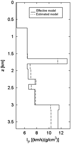
Figure 21 S-wave impedances I_S vs. the depth z; comparison between the effective model (solid line) and the estimated model (dashed line).

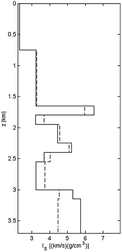
Figure 22 P-wave velocities v_P vs. the depth z; comparison between the effective model (solid line) and the estimated model (dashed line).

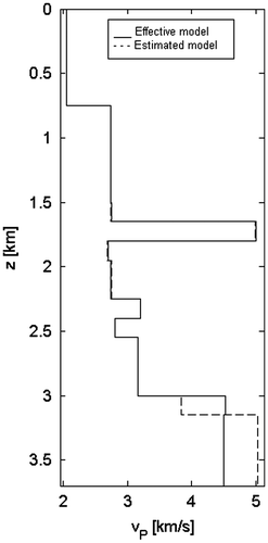
Figure 23 S-wave velocities v_S vs. the depth z; comparison between the effective model (solid line) and the estimated model (dashed line).

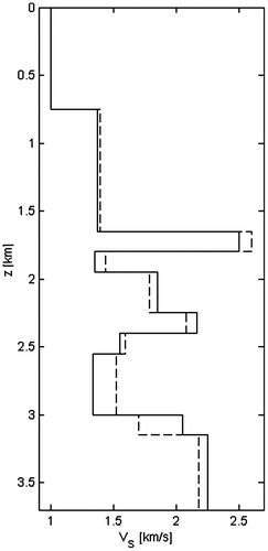
Figure 24 Rock densities ρ vs. the depth z; comparison between the effective model (solid line) and the estimated model (dashed line).

The results obtained in these seismic inversion examples show how the distance indicator can be helpfully used in order to discuss the re-parameterization of the model space. This method is attractive, especially, if applied to the inverse problems where the null-space is not perfectly known and where a conditioning analysis is difficult to obtain.

6 Conclusions

The solution of non-linear inverse problems could result in unsatisfactory retrieved models when a local search approach is adopted and an exhaustive exploration is not viable because of the problem dimensions. Indeed, a parsimonious exploration of the model space is necessary when using global optimizer in applications where the cost function is highly multimodal and therefore the convergence of the solution and its properties, such as the detection of the local minima and the influence of constraints or a priori knowledge, are particularly demanding.

The main result of this paper is that the use of a distance indicator, defined as the Euclidian distance in the model space, helps in following the evolution of a global optimizer, even in those cases in which a visual representation of the function to optimize is not viable, i.e. the dimensions of variable space are greater than three. The key of this approach is that the distance indicator clearly identifies the region near the optimum. At this stage, one could stop the iterative calculations of the global optimizer and solve the problem through local optimization.

To illustrate the performance of such an approach, three problems with different degree of complexity were chosen ranging from optimal signal alignment to geophysical parameters inversion, through global optimization based upon the SAA. In all the examples, the Euclidean distance proved to be a useful tool in describing the evolution of the object function.

Acknowledgements

The authors would like to thank one of the reviewers for his suggestion to deepen the discussion about the motivation in choosing the Euclidian distance from a reference point as a metric. He suggested investigating different norms and approximations of the reference point. These issues will stimulate our future work.

Notes

This article was originally published with errors. This version has been amended. Please see Corrigendum (http://dx.doi.org/10.1080/17415977.2014.918742)

Appendix 1.

Optimization with a global algorithm based on the concept of distance

The global optimization performed by the SAA is computationally cumbersome, especially in the final step of the optimizing procedure, where the domain of the variable space containing the best local optimum has already been identified. Therefore, it is welcome to quit the algorithm at this stage and to adopt a hybrid strategy, thus decreasing considerably the total computational cost.

The chosen approach combines SAA with the gradient method and it executes two main steps:

1. exploration of the domain of the objective function and localization of the model domain where the probability to find the global optimum is high; this leads to the identification of a model domain with only one optimum (stopped simulated annealing).

2. inverse problem solution through local optimization having set as guess the optimum solution singled out at the step 1.

The hybrid and the original implementations of the SAA have the same nested cycle’s structure and they both evaluate NF times the error function f to be optimized:(A1) $N_{\text{F}}=M\times N_{\text{S}}\times N_{\text{T}}\times N_{\text{R}}$(A1)

This is an index of the computational cost and it depends on M, the dimensions of the variable space, on N_S and N_T, constants chosen with the strategy of Corana [9] and on N_R, the number of temperature reductions.

The hybrid algorithm stops at the end of the step 1, whence N_R and N_F are smaller of the corresponding values given by the standard approach. In particular, N_F is a computational index of the complete inversion process because it is far higher than the cost of the linear optimization employed at the step 2 to refine the solution.

If i is the index denoting the model parameters (i = 1, … , M), j denotes the successive points for each temperature reduction ($j=1\text{,}\dots \text{,}M\times N_{\text{S}}\times N_{\text{T}}$) and k covers successive temperature reductions ($k=1\text{,}\dots \text{,}{N}_{\text{R}}$), then the point j of the variable space, evaluated at the temperature reduction k, is denoted by m_jk and the corresponding model parameter i is m_ijk.

The solution of the forward problem, described by the non-linear function g, for an estimated model vector m_jk, is the vector:(A2) ${\mathit{y}}_{\mathit{jk}}=g({\mathit{m}}_{\mathit{jk}})$(A2)

For each particular iteration j and temperature reduction k, the error function is sampled and its square value is equal to:(A3) $f_{\mathit{jk}}=\sum _{n=1}^N(g_{\text{obs,}n}-y_{\mathit{njk}}{)}^2$(A3)

with $y_{\mathit{njk}}$, the component n of the ${\mathit{y}}_{\mathit{jk}}$ vector, $g_{\text{obs,}n}$ the component n of g_obs, the observed data vector and N the dimensions of the data space ($n=1\text{,}\dots \text{,}N$).

a and b are the vectors of the lower and upper bounds of the model domain:(A4) $\begin{array}{c}\hfill a_1<m_1<b_1\hfill \\ \hfill a_2<m_2<b_2\hfill \\ \hfill \cdots \hfill \\ \hfill a_{\text{M}}<m_{\text{M}}<b_{\text{M}}\hfill \end{array}$(A4)

r = b – a is called range vector because it represents the maximum range of the model parameters, which is also the distance between the upper and the lower bounds.

The stopping criterion is based on the geometric concept of distance. At the jth iteration of the kth temperature reduction, the square of the distance is:(A5) $d_{\mathit{jk}}^2=\sum _{i=1}^M{p}_i^2(m_{\mathit{ijk}}-m_{\text{ref,}i}{)}^2$(A5)

with $m_{\text{ref,}i}$ the component i of a reference point ${\mathit{m}}_{\text{ref}}$.

The vector of the weights p, used to normalize the inhomogeneous model parameters, is calculated as:(A6) $p_i=\frac{r_{\text{max}}}{r_i}$(A6)

being r_max the maximum value among the components of the range vector. When a model parameter is larger than the other ones, this ratio tends to 1; on the other side, when a model parameter is smaller than the others, p_i ≫ 1: all the model parameters thus contribute to the distance calculation as they were homogeneous quantities.

The optimal distance, d_opt,k, corresponding to the distance in the variable space between the optimum point m_opt,k and the reference point m_ref, the smallest distance d_min,k, the largest distance d_max,k and ${\sigma }_k^2$, a measure of the distance dispersion around d_opt,k, are then computed:(A7) $\begin{array}{c}\hfill d_{\text{opt,}k}^2=\sum _{i=1}^M{p}_i^2(m_{\text{opt,}\mathit{ik}}-m_{\text{ref,}i}{)}^2\hfill \\ \hfill d_{\max \text{,}k}=\underset{j\text{;}l=1\text{,}\dots \text{,}k}{\max }(d_{\mathit{jl}})\hfill \\ \hfill d_{\min \text{,}k}=\underset{j\text{;}l=1\text{,}\dots \text{,}k}{\min }(d_{\mathit{jl}})\hfill \\ \hfill {\mathit{range}}_k=d_{\max \text{,}k}-d_{\min \text{,}k}\hfill \\ \hfill {\sigma }_k^2=\frac{1}{N_{\text{d}}}\sum _{j=1}^{N_{\text{d}}}(d_{\mathit{jk}}-d_{\text{opt,}k}{)}^2\hfill \end{array}$(A7)

The best optimum for the hybrid algorithm is found when ${\sigma }_k⩽{\epsilon }_{\text{d}}\times {\mathit{range}}_k$, called sensitivity on the convergence criterion, is a parameter set by the user. We recommend choosing ${\epsilon }_{\text{d}}$ in the range from 10⁻³ to 10⁻¹.

Then, the solution is refined by a local optimization, starting from the model point of the best previously found solution.

References

- Tarantola A. Inverse problem theory. Philadelphia, PA: SIAM; 2004.
- Mosegaard K, Tarantola A. Monte carlo sampling of solutions to inverse problems. J. Geophys. Res. 1995;100:431–447.
- Locatelli M. Convergence properties of simulated annealing for continuous global optimization. J. Appl. Probab. 1996;33:1127–1140. Available from: http://www.jstor.org/stable/3214991.
- Gilbert JCh, Nocedal J. Global convergence properties of conjugate gradient methods for optimization. Siam J. Optim. 1992;2:21–42.
- Storn R, Price K. Differential evolution – a simple and efficient adaptive scheme for global optimization over continuous spaces. Technical Report TR-95-012, ICSI, Mar 1995, ftp.icsi.berkeley.edu.
- Rocca P, Benedetti M, Donelli M, Franceschini D, Massa A. Evolutionary optimization as applied to inverse scattering problems. Inverse Prob. 2009;25:1–41. doi:10.1088/0266-5611/25/12/123003.
- Mingjun Ji, Klinowski J. Convergence of taboo search in continuous global optimization. Proc. R. Soc. A. 2006;462:2077–2084. doi:10.1098/rspa.2006.1678.
- Xinchao Z. A greedy genetic algorithm for unconstrained global optimization. J. Syst. Sci. Complexity. 2005;18:102–110.
- Corana A, Marchesi M, Martini C, Ridella S. Minimizing multimodal functions of continuous variables with the simulated annealing algorithm. ACM Trans. Math. Softw. 1987;13:262–280.
- Goffe WL. SIMANN: a global optimization algorithm using simulated annealing, studies in nonlinear dynamics and econometrics. Quart. J. 1996;1:169–173.
- Purushothama GK, Jenkins L. Simulated annealing with local search – a hybrid algorithm for unit commitment. IEEE Trans. Power Syst. 2003;18:273–278.
- Rovetta D. Applicazioni a problemi di inversione non lineare : simulated annealing [Master thesis]. Milan: Politecnico di Milano; 2002.
- Rovetta D. Inverse problem analysis [PhD dissertation]. Milan: Politecnico Di Milano; 2006.
- Rothmann DH. Large near-surface anomalies, seismic reflection data and simulated annealing [PhD dissertation]. SEP, Stanford (CA); October 1985.
- Bosisio AV, Drufuca G. Retrieval of two-dimensional absorption coefficient structure from a scanning radiometer at 23.8 GHz. Radio Sci. 2003;38:3.1–3.9. doi:10.1029/2002RS002628.
- Ulaby FT, Moore RK, Fung AK. Microwave remote sensing volume I: microwave remote sensing fundamentals and radiometry. Reading, MA: Addison Wesley; 1981.
- Bean BR, Dutton EJ. Radio meteorology. New York: Dover; 1968.
- Kak AC. Principles of computerized tomographic imaging. New York: IEEE Press; 1988.
- Salonen E, Karhu S, Jokela P, Zhang W, Uppsala S, Alamo H, Sarkkula S. Study of propagation phenomena for low availabilities, Appendix A – Standard Atmospheres, ESTEC 8025/88/NL/PR Final report, Norwijck (NL); 1990.
- Ma XQ. A constrained global inversion method using an over-parameterized scheme: application to poststack seismic data. Geophysics. 2001;66:613–626.
- Ma XQ. Simultaneous inversion of prestack seismic data for rock properties using simulated annealing. Geophysics. 2002;67:1877–1885.
- Becquey M, Lavergne M, Willm C. Acoustic impedance logs computed from seismic traces. Geophysics. 1979;44:1485–1501.
- Oldenburg D, Scheuer T, Levy S. Recovery of acoustic impedance from reflection seismograms. Geophysics. 1983;48:1318–1337.
- Fuchs K, Müller G. Computation of synthetic seismograms with the reflectivity method and comparison with observations. Geophys. J. R. Astr. Soc. 1971;23:417–433.
- Pilant WL. Elastic waves in the earth. Amsterdam: Elsevier; 1979.
- Ramo S, Whinnery JR, Van Duzer T. Fields and waves in communication electronics. New York, NY: Wiley; 1965.