Inversion of weighted Radon transforms via finite Fourier series weight approximations

Abstract

We consider weighted Radon transforms on the plane. We show that the Chang approximate inversion formula for these transforms admits a significant extension as inversion via finite Fourier series weight approximations. We illustrate this inversion approach by numerical examples for the case of the attenuated Radon transforms in the framework of the single-photon emission computed tomography (SPECT).

Keywords:

• weighted radon transforms
• emission tomography
• approximate inversion algorithms
• Chang’s formula
• finite Fourier series weight approximations

Introduction

The basic problem of many tomographies consists of finding an unknown function f on ${\mathbb{R}}^2$ from its weighted ray transform $P_{W}f$ on $\mathbb{R}\times {\mathbb{S}}^1$ for some known weight W, where(1.1) $$\begin{array}{c}\hfill \begin{array}{c}{P}_{W}f(s,\mathit{\theta })=\underset{\mathbb{R}}{\int }W(s{\mathit{\theta }}^{\perp }+t\mathit{\theta },\mathit{\theta })f(s{\mathit{\theta }}^{\perp }+t\mathit{\theta })\mathit{dt},\hfill \\ s\in \mathbb{R},\mathit{\theta }=({\mathit{\theta }}_1,{\mathit{\theta }}_2)\in {\mathbb{S}}^1,{\mathit{\theta }}^{\perp }=(-{\mathit{\theta }}_2,{\mathit{\theta }}_1),\hfill \end{array}\end{array}$$(1.1) where $f=f(x)$, $W=W(x,\mathit{\theta })$, $x\in {\mathbb{R}}^2$. Up to change of variables, the operator $P_W$ is known also in literature as the weighted Radon transform on the plane. In this work we always assume that(1.2) $$\begin{array}{cc}\hfill & W\in C({\mathbb{R}}^2\times {\mathbb{S}}^1)\cap L^{\infty }({\mathbb{R}}^2\times {\mathbb{S}}^1),\hfill \\ \hfill & w_0(x)\frac{\mathrm{def}}{\mathrm{=}}\frac{1}{2\mathit{\pi }}\underset{{\mathbb{S}}^1}{\int }W(x,\mathit{\theta })d\mathit{\theta }\ne 0,x\in {\mathbb{R}}^2,\hfill \end{array}$$(1.2) where W is complex valued, in general, and $d\mathit{\theta }$ is the standard element of arc length on ${\mathbb{S}}^1$. Additional assumptions on W will be formulated in the framework of context. In particular, in important cases, W is real valued and strictly positive:(1.3) $$\begin{array}{c}\hfill \begin{array}{c}W=\overline{W},W\ge c>0.\hfill \end{array}\end{array}$$(1.3) In addition, for this work one can always assume that(1.4) $$\begin{array}{c}\hfill \begin{array}{c}f\in L^{\infty }\left({\mathbb{R}}^2\right),\mathit{supp}f\subset D,\hfill \end{array}\end{array}$$(1.4) where f is complex valued, in general, and D is an open bounded domain (which is fixed a priori).

In definition (1.1), the product $\mathbb{R}\times {\mathbb{S}}^1$ is interpreted as the set of all oriented straight lines in ${\mathbb{R}}^2$. If $\mathit{\gamma }=(s,\mathit{\theta })\in \mathbb{R}\times {\mathbb{S}}^1$, then $\mathit{\gamma }=\{x\in {\mathbb{R}}^2:x=s{\mathit{\theta }}^{\perp }+t\mathit{\theta },t\in \mathbb{R}\}$ (modulo orientation) and $\mathit{\theta }$ gives the orientation of $\mathit{\gamma }$.

If $W\equiv 1$, then $P_W$ is reduced to classical ray (or Radon) transform on the plane. If(1.5) $$\begin{array}{c}\hfill W(x,\mathit{\theta })=\exp (-\underset{0}{\overset{+\infty }{\int }}a(x+t\mathit{\theta })\mathit{dt}),\end{array}$$(1.5) where a is a complex-valued sufficiently regular function on ${\mathbb{R}}^2$ with sufficient decay at infinity, then $P_W$ is known in literature as the attenuated ray (or Radon) transform on the plane.

The classical ray transform arises, in particular, in X-ray transmission tomography, see e.g. [1]. The attenuated ray transform (at least, with real-valued $a\ge 0$) arises, in particular, in SPECT, see e.g. [1, 2]. Transforms $P_W$ with some other weights also arise in applications, see e.g. [2–5].

Exact and simultaneously explicit inversion formulas for the classical and attenuated ray (or Radon) transforms on the plane were given for the first time in [6] and [7], respectively. For some other weights W, exact and simultaneously explicit inversion formulas were given in [8–11]. Note that, we say that an inversion method for $P_W$ is an explicit inversion formula if its complexity is comparable with complexity of the aforementioned Radon inversion formula of [6]. In this sense, the analytic inversion method for the attenuated ray transform proposed before [7] in [12] is not an explicit inversion formula: the inversion of [12] is not better than an infinite series, where each term is not simpler than the classical Radon inversion formula.

Apparently, for general $P_W$, under assumptions (1.2), (1.3), explicit and simultaneously exact (modulo $\mathit{Ker}{P}_W$) inversion formulas are impossible. In addition, [13] gives an example of infinitely smooth W satisfying (1.2), (1.3) and such that $\mathit{Ker}{P}_W\ne 0$ in the space of infinitely smooth compactly supported functions on ${\mathbb{R}}^2$. But, due to [14], $\mathit{Ker}{P}_W=0$ in the space of continuous compactly supported functions on ${\mathbb{R}}^2$ for real analytic W satisfying (1.3).

On the other hand, the following Chang approximate (but explicit) inversion formula for $P_W$, where W is given by (1.5) with $a\ge 0$, has been used for a long time (see e.g. [2, 11, 15]):(1.6) $$\begin{array}{c}\hfill \begin{array}{c}{f}_{\mathit{appr}}={(w_0)}^{-1}{P}^{-1}{P}_{W}f,\hfill \end{array}\end{array}$$(1.6) where $w_0$ is defined in (1.2), $P^{-1}$ denotes the classical Radon inversion realized via the formula given below:(1.7) $$\begin{array}{cc}\hfill & P^{-1}q(x)=\frac{1}{4\mathit{\pi }}\underset{{\mathbb{S}}^1}{\int }{\mathit{\theta }}^{\perp }{\nabla }_x(\frac{1}{\mathit{\pi }}p.v.\underset{\mathbb{R}}{\int }\frac{q(t,\mathit{\theta })}{x{\mathit{\theta }}^{\perp }-t}\mathit{dt})d\mathit{\theta },x\in {\mathbb{R}}^2,\hfill \\ \hfill & {\mathit{\theta }}^{\perp }{\nabla }_x=-{\mathit{\theta }}_2\mathit{\partial }/\mathit{\partial }{x}_1+{\mathit{\theta }}_1\mathit{\partial }/\mathit{\partial }{x}_2,x{\mathit{\theta }}^{\perp }=-{\mathit{\theta }}_2{x}_1+{\mathit{\theta }}_1{x}_2,\mathit{\theta }=({\mathit{\theta }}_1,{\mathit{\theta }}_2),x=(x_1,x_2),\hfill \end{array}$$(1.7) where q is a test function on $\mathbb{R}\times {\mathbb{S}}^1$. It is known that formula (1.6) is efficient for the first approximation in SPECT reconstructions and, in particular, is sufficiently stable for reconstruction from discrete data with strong Poisson noise. The exact inversion formula of [7] for the attenuated ray transform is considerably less stable in this respect. For more information in this connection see [16].

Formula (1.6), under assumptions (1.2), can be considered as approximate inversion of $P_W$ via the approximation(1.8) $$\begin{array}{c}\hfill \begin{array}{c}W(x,\mathit{\theta })\approx w_0(x),x\in {\mathbb{R}}^2,\mathit{\theta }\in {\mathbb{S}}^1,\hfill \end{array}\end{array}$$(1.8) i.e. via the zero term Fourier approximation for W in angle variable. In addition, due to [6], formula (1.6) is exact if(1.9) $$\begin{array}{c}\hfill \begin{array}{c}W(x,\mathit{\theta })\equiv w_0(x),x\in {\mathbb{R}}^2,\mathit{\theta }\in {\mathbb{S}}^1.\hfill \end{array}\end{array}$$(1.9) Besides, due to [11], formula (1.6) is exact if and only if(1.10) $$\begin{array}{c}\hfill \begin{array}{c}W(x,\mathit{\theta })-w_0(x)\equiv w_0(x)-W(x,-\mathit{\theta }),x\in {\mathbb{R}}^2,\mathit{\theta }\in {\mathbb{S}}^1.\hfill \end{array}\end{array}$$(1.10) However, already for W of (1.5) property (1.10) is not fulfilled, in general.

In the present work, we consider approximate inversion of $P_W$ via the approximations(1.11) $$\begin{array}{cc}\hfill & W(x,\mathit{\theta }(\mathit{\phi }))\approx \sum _{n=-N}^N{e}^{\mathit{in}\mathit{\phi }}{w}_n(x),\hfill \\ \hfill & w_n(x)=\frac{1}{2\mathit{\pi }}\underset{-\mathit{\pi }}{\overset{\mathit{\pi }}{\int }}{e}^{-\mathit{in}\mathit{\phi }}W(x,\mathit{\theta }(\mathit{\phi }))d\mathit{\phi },\hfill \\ \hfill & x\in {\mathbb{R}}^2,\mathit{\theta }(\mathit{\phi })=(\cos \mathit{\phi },\sin \mathit{\phi }),\mathit{\phi }\in [-\mathit{\pi },\mathit{\pi }],N\in \mathbb{N}\cup 0.\hfill \end{array}$$(1.11) One can see that for $N=0$ approximation (1.11) is reduced to (1.8).

Our approximate inversion algorithms for $P_W$ on functions of (1.4), under general assumptions (1.2), are presented in Subsection 2.4 of Section 2 , see approximate inversions (2.20), (2.22). In particular, one can consider that $N=2m+1$, where N is the approximation number of (1.11) and m is the maximal number of (2.22). In these considerations, we proceed from [2] and [17].

In Section 3, our approximate inversions (2.20), (2.22) of Subsection 2.4 are illustrated by numerical examples for specific W given by (1.5) with $a\ge 0$ in the framework of SPECT.

Finally, note that the ‘philosophy’ of our approach to approximate inversion of $P_W$ via the approximations (1.11) is actually similar to the ‘philosophy’ described in [18, 19] for the case of coefficient inverse problems. More precisely: we replace the exact model by its approximations (via (1.11) in our case) and for the approximate model, we solve the problem by iterations with good properties (via (2.22) in our case). Next, we show that such a solution is good enough for the initial non-approximative model (see Subsection 3.5).

Approximate inversion of $P_W$

Symmetrization of W

Let(2.1) $$\begin{array}{c}\hfill \begin{array}{c}{A}_{W}f=P^{-1}{P}_{W}f,\hfill \end{array}\end{array}$$(2.1) where $P^{-1}$ is defined by (1.7). Let(2.2) $$\begin{array}{c}\hfill \begin{array}{c}{W}_{\mathit{sym}}(x,\mathit{\theta })=\frac{1}{2}(W(x,\mathit{\theta })+W(x,-\mathit{\theta })),x\in {\mathbb{R}}^2,\mathit{\theta }\in {\mathbb{S}}^1.\hfill \end{array}\end{array}$$(2.2) We consider also the Fourier series(2.3) $$\begin{array}{cc}\hfill & W(x,\mathit{\theta }(\mathit{\phi }))=\sum _{n=-\infty }^{+\infty }{e}^{\mathit{in}\mathit{\phi }}{w}_n(x),x\in {\mathbb{R}}^2,\mathit{\phi }\in [-\mathit{\pi },\mathit{\pi }],\hfill \end{array}$$(2.3) where $w_n$ is defined in (1.11), $\mathit{\theta }(\mathit{\phi })=(\cos \mathit{\phi },\sin \mathit{\phi })$.

The following formulas hold (see [2, 11]):(2.4) $$\begin{array}{cc}\hfill & \frac{1}{2}(P_{W}f(s,\mathit{\theta })+P_{W}f(-s,-\mathit{\theta }))=P_{W_{\mathit{sym}}}f(s,\mathit{\theta }),(s,\mathit{\theta })\in \mathbb{R}\times {\mathbb{S}}^1,\hfill \end{array}$$(2.4) (2.5) $$\begin{array}{cc}\hfill & A_{W}f=P^{-1}{P}_{W_{\mathit{sym}}}f,\hfill \end{array}$$(2.5) (2.6) $$\begin{array}{cc}\hfill & W_{\mathit{sym}}(x,\mathit{\theta }(\mathit{\phi }))=\sum _{l=-\infty }^{+\infty }{e}^{i2l\mathit{\phi }}{w}_{2l}(x),x\in {\mathbb{R}}^2,\mathit{\phi }\in [-\mathit{\pi },\mathit{\pi }].\hfill \end{array}$$(2.6) Actually, using (2.4)–(2.6) we reduce inversion of $P_W$ to inversion of $P_{W_{\mathit{sym}}}$. In particular, using (2.1), (2.5), (2.6), one can see that such reduction arises already in the framework of (1.6).

Operators $Q_{W,D,m}$ and numbers ${\mathit{\sigma }}_{W,D,m}$

Consider(2.7) $$\begin{array}{c}\hfill z=x_1+{\mathit{ix}}_2,\overline{z}=x_1-{\mathit{ix}}_2,x=(x_1,x_2)\in {\mathbb{R}}^2.\end{array}$$(2.7) Using (2.7), we identify ${\mathbb{R}}^2$ with $\mathbb{C}$.

Let $\mathrm{\Pi }$, $\overline{\mathrm{\Pi }}$ denote the linear integral operators on ${\mathbb{R}}^2$ identified with $\mathbb{C}$ such that(2.8) $$\begin{array}{c}\hfill \mathrm{\Pi }u(z)=-\frac{1}{\mathit{\pi }}\underset{\mathbb{C}}{\int }\frac{u(\mathit{\zeta })}{{(\mathit{\zeta }-z)}^2}\mathit{dRe}\mathit{\zeta }\mathit{dIm}\mathit{\zeta },\\ \hfill \overline{\mathrm{\Pi }}u(z)=-\frac{1}{\mathit{\pi }}\underset{\mathbb{C}}{\int }\frac{u(\mathit{\zeta })}{{(\overline{\mathit{\zeta }}-\overline{z})}^2}\mathit{dRe}\mathit{\zeta }\mathit{dIm}\mathit{\zeta },\end{array}$$(2.8) where u is a test function, $z\in \mathbb{C}$; see e.g. [20] for detailed properties of these operators.

Let D be the domain of (1.4).

Let ${\mathit{\chi }}_D$ denote the characteristic function of D, i.e.(2.9) $$\begin{array}{c}\hfill {\mathit{\chi }}_D\equiv 1\mathrm{on}D,{\mathit{\chi }}_D\equiv 0\mathrm{on}{\mathbb{R}}^2\setminus D.\end{array}$$(2.9) Let(2.10) $$\begin{array}{cc}\hfill Q_{W,D,m}& =\sum _{l=1}^m({(-\overline{\mathrm{\Pi }})}^l\frac{w_{2l}}{w_0}+{(-\mathrm{\Pi })}^l\frac{w_{-2l}}{w_0}){\mathit{\chi }}_D\mathrm{for}m\in \mathbb{N},\hfill \\ \hfill Q_{W,D,m}& =0\mathrm{for}m=0,\hfill \end{array}$$(2.10) where $w_0$, $w_{2l}$ are the Fourier coefficients of (2.3), (2.6) and $w_{\pm 2l}/w_0$, ${\mathit{\chi }}_D$ are considered as the multiplication operators of ${\mathbb{R}}^2$.

Let(2.11) $$\begin{array}{cc}\hfill {\mathit{\sigma }}_{W,D,m}& =\sum _{l=1}^m\left(\underset{x\in D}{\sup }\right|\frac{w_{2l}(x)}{w_0(x)}|+\underset{x\in D}{\sup }|\frac{w_{-2l}(x)}{w_0(x)}\left|\right)\mathrm{for}m\in \mathbb{N},\hfill \\ \hfill {\mathit{\sigma }}_{W,D,m}& =0\mathrm{for}m=0.\hfill \end{array}$$(2.11) According to [17] we have that(2.12) $$\begin{array}{c}\hfill \begin{array}{c}\parallel Q_{W,D,m}{\parallel }_{L^2({\mathbb{R}}^2)\to L^2({\mathbb{R}}^2)}\le {\mathit{\sigma }}_{W,D,m}.\hfill \end{array}\end{array}$$(2.12)  

Exact inversion for finite Fourier series weights

Let conditions (1.2), (1.4) be fulfilled and(2.13) $$\begin{array}{cc}\hfill & W(x,\mathit{\theta }(\mathit{\phi }))=\sum _{n=-N}^N{e}^{\mathit{in}\mathit{\phi }}{w}_n(x),\hfill \\ \hfill & x\in {\mathbb{R}}^2,\mathit{\theta }(\mathit{\phi })=(\cos \mathit{\phi },\sin \mathit{\phi }),\mathit{\phi }\in [-\mathit{\pi },\mathit{\pi }],N\in \mathbb{N}\cup 0.\hfill \end{array}$$(2.13) Suppose also that(2.14) $$\begin{array}{c}\hfill {\mathit{\sigma }}_{W,D,m}<1\mathrm{for}m=[N/2],\end{array}$$(2.14) where $[N/2]$ denotes the integer part of $N/2$. Then according to [17], we have the following exact inversion for $P_W$:(2.15) $$\begin{array}{c}\hfill f={(w_0)}^{-1}{(I+Q_{W,D,m})}^{-1}{P}^{-1}{P}_{W}f,\end{array}$$(2.15) where I is the identity operator on ${\mathbb{R}}^2$, $P^{-1}$ is defined by (1.7). In addition, in view of (2.12), (2.14) we have that(2.16) $$\begin{array}{c}\hfill {(I+Q_{W,D,m})}^{-1}=I+\sum _{j=1}^{+\infty }{(-Q_{W,D,m})}^j.\end{array}$$(2.16) In addition, under our assumptions, we have that (see [17]):(2.17) $$\begin{array}{c}\hfill A_{W}f=P^{-1}{P}_{W}f\in L^2({\mathbb{R}}^2).\end{array}$$(2.17)  

Approximate inversion for general weights

Let conditions (1.2), (1.4) be fulfilled and(2.18) $$\begin{array}{c}\hfill \sum _{l=1}^{\infty }(\parallel \frac{w_{2l}}{w_0}{\parallel }_{L^2(D)}+\parallel \frac{w_{-2l}}{w_0}{\parallel }_{L^2(D)})<+\infty ,\end{array}$$(2.18) where $w_n$ are defined by (2.11). Suppose that(2.19) $$\begin{array}{c}\hfill {\mathit{\sigma }}_{W,D,m}\le {\mathit{\sigma }}_{\max }<1\mathrm{for}\mathrm{fixed}m\in \mathbb{N}\cup 0.\end{array}$$(2.19) Then we consider that(2.20) $$\begin{array}{cc}\hfill & f\approx f_m,\hfill \\ \hfill & f_m={(w_0)}^{-1}{(I+Q_{W,D,m})}^{-1}{P}^{-1}{P}_{W}f,\hfill \end{array}$$(2.20) where I is the identity operator, $Q_{W,D,m}$ is defined by (2.10), $P^{-1}$ is defined by (1.7). Note that the right-hand side of (2.20b) is well-defined: in particular, in view of (2.12), (2.19) we have formula (2.16) in norm $\parallel ·{\parallel }_{L^2({\mathbb{R}}^2)\to L^2({\mathbb{R}}^2)}$ and using (2.18) one can show that(2.21) $$\begin{array}{c}\hfill P^{-1}{P}_{W}f\in L^2({\mathbb{R}}^2).\end{array}$$(2.21) Formula (2.20) is a natural extension of the Chang formula (1.6). In particular, (2.20) for $m=0$ coincides with (1.6).

In addition, if (2.19) is fulfilled for some $m\ge 1$, then $f_m$ is a refinement of the Chang approximation $f_0$ and, more generally, $f_j$ is a refinement of $f_i$ for $0\le i<j\le m$. But of course $f_j=f_i$ if $w_{2l}\equiv 0$, $w_{-2l}\equiv 0$ for $i<l\le j$.

Actually, in many important examples condition (2.19) is efficiently fulfilled for small m (e.g. $m=2$) and is not fulfilled for large m. Therefore, in the present work, under conditions (1.2)-(1.4), we propose the following approximate reconstruction of f from $P_{W}f$:(2.22) $$\begin{array}{c}\hfill \begin{array}{c}\mathrm{find}\mathrm{maximal}m\mathrm{such}\mathrm{that}(2.19)\mathrm{is}\mathrm{still}\mathrm{fulfilled}\hfill \\ \mathrm{and}\mathrm{approximately}\mathrm{reconstruct}f\mathrm{via}(2.20)\mathrm{using}(2.12),(2.16).\hfill \end{array}\end{array}$$(2.22) In Section 3, we illustrate this approximate reconstruction by numerical examples in the framework of SPECT with ${\mathit{\sigma }}_{\max }=0.7$. In particular, these numerical examples show that stability properties of this approximate reconstruction $f_m$ are similar to stability properties of the Chang approximate reconstruction $f_0$ but $f_m$ is more precise than $f_0$ if $m>0$.

Note also that using considerations presented below in Subsection 2.5 and considerations presented at the end of Section 5 of [2], algorithm (2.22) can be designed on the basis of the 2D FFT.

Using considerations of Subsection 2.3, one can see also that(2.23) $$\begin{array}{c}\hfill f=f_m-{(w_0)}^{-1}{(I+Q_{W,D,m})}^{-1}{P}^{-1}{P}_{\mathit{\delta }{W}_m}f,\end{array}$$(2.23) where(2.24) $$\begin{array}{cc}\hfill & \mathit{\delta }{W}_m(x,\mathit{\theta }(\mathit{\phi }))\frac{\mathrm{def}}{\mathrm{=}}W(x,\mathit{\theta }(\mathit{\phi }))-\sum _{n=-2m-1}^{2m+1}{e}^{\mathit{in}\mathit{\phi }}{w}_n(x),\hfill \\ \hfill & x\in {\mathbb{R}}^2,\mathit{\theta }(\mathit{\phi })=(\cos \mathit{\phi },\sin \mathit{\phi }),\mathit{\phi }\in [-\mathit{\pi },\mathit{\pi }],m\in \mathbb{N}\cup 0,\hfill \end{array}$$(2.24) where $w_n$ are defined by (1.11). One can use (2.23) for estimating the error $f-f_m$. One can also consider (2.23) as an integral equation for finding f from $f_m$. Note also that Equation (2.23) for $m=0$ is, actually, well known, see e.g. [2].

Relations with [2]

Let conditions (1.2), (1.4) be fulfilled and(2.25) $$\begin{array}{c}\hfill \underset{m\to +\infty }{\lim }{\mathit{\sigma }}_{W,D,m}={\mathit{\sigma }}_{W,D}<+\infty .\end{array}$$(2.25) Then, we can consider(2.26) $$\begin{array}{c}\hfill Q_{W,D}=\underset{m\to +\infty }{\lim }{Q}_{W,D,m}\mathrm{in}\parallel ·{\parallel }_{L^2({\mathbb{R}}^2)\to L^2({\mathbb{R}}^2)}.\end{array}$$(2.26) In addition, if(2.27) $$\begin{array}{c}\hfill {\mathit{\sigma }}_{W,D}<1,\end{array}$$(2.27) then(2.28) $$\begin{array}{c}\hfill f={(w_0)}^{-1}{(I+Q_{W,D})}^{-1}{P}^{-1}{P}_{W}f,\end{array}$$(2.28) (2.29) $$\begin{array}{c}\hfill {(I+Q_{W,D})}^{-1}=I+\sum _{j=1}^{+\infty }{(-Q_{W,D})}^j.\end{array}$$(2.29) Actually, (2.28) is a linear integral equation for exact reconstruction of f from $P_{W}f$ under assumptions (1.2), (1.4), (2.18), (2.27). In addition, (2.29) can be interpreted as the method of successive approximations for solving this equation.

It is possible to show that the reconstruction of f from $P_{W}f$ of [2] (or, more precisely, the linear integral equation on $\mathit{\epsilon }$ on page 814 of [2]) can be transformed into (2.28).

In [2] (under the assumption that $0<W<1$), it was shown that this equation on $\mathit{\epsilon }$ of [2] is uniquely solvable if(2.30) $$\begin{array}{cc}\hfill & \underset{m\to +\infty }{\lim }{\mathit{\rho }}_{W,D,m}={\mathit{\rho }}_{W,}D<1,\hfill \\ \hfill & {\mathit{\rho }}_{W,D,m}\frac{\mathrm{def}}{\mathrm{=}}\frac{\sum _{l=1}^m(\underset{x\in D}{\sup }|w_{2l}(x)|+\underset{x\in D}{\sup }|w_{-2l}(x)|)}{\underset{x\in D}{\min }|w_0(x)|}.\hfill \end{array}$$(2.30) One can see that in many cases, ${\mathit{\sigma }}_{W,D,m}$ is much smaller than ${\mathit{\rho }}_{W,D,m}$ and our condition (2.27) is much less restrictive than (2.30) of [2].

Under assumption (2.30), finite Fourier series weight approximations (1.11) are also considered at the end of Section 5 of [2] in the framework of approximate but rapid inversion of weighted Radon transforms on the basis of the 2D FFT.

In addition, the most important difference between our algorithm (2.22) and the inversion algorithms of [2] consists in the following: we suggest algorithm (2.22) for general weights W satisfying (1.2), (1.3), whereas the algorithms of [2] are suggested under very restrictive smallness assumption (2.30) only.

Actually, in order to relate considerations of [2] on one hand with considerations of [17] and the present work on the other hand, we use the following formulas(2.31) $$\begin{array}{c}\hfill \begin{array}{c}\mathcal{F}({\mathrm{\Pi }}^{l}u)(\mathit{\xi })={\left(\frac{{\mathit{\xi }}_1-i{\mathit{\xi }}_2}{{\mathit{\xi }}_1+i{\mathit{\xi }}_2}\right)}^l\mathcal{F}u(\mathit{\xi }),\hfill \\ \mathcal{F}({\overline{\mathrm{\Pi }}}^{l}u)(\mathit{\xi })={\left(\frac{{\mathit{\xi }}_1+i{\mathit{\xi }}_2}{{\mathit{\xi }}_1-i{\mathit{\xi }}_2}\right)}^l\mathcal{F}u(\mathit{\xi }),\hfill \\ \mathit{\xi }=({\mathit{\xi }}_1,{\mathit{\xi }}_2)\in {\mathbb{R}}^2,l\in \mathbb{N},\hfill \end{array}\end{array}$$(2.31) (2.32) $$\begin{array}{cc}\hfill Q_{W,D,m}u(x)=& P^{-1}(P_{W,D,m}u)(x),\hfill \\ \hfill P_{W,D,m}u(s,\mathit{\theta })\frac{\mathrm{def}}{\mathrm{=}}& \underset{\mathbb{R}}{\int }\left((\sum _{l=-m}^{-1}+\sum _{l=1}^m)\frac{w_{2l}(s{\mathit{\theta }}^{\perp }+t\mathit{\theta })}{w_0(s{\mathit{\theta }}^{\perp }+t\mathit{\theta })}{({\mathit{\theta }}_1+i{\mathit{\theta }}_2)}^{2l}\right)\hfill \\ \hfill & \times {\mathit{\chi }}_D(s{\mathit{\theta }}^{\perp }+t\mathit{\theta })u(s{\mathit{\theta }}^{\perp }+t\mathit{\theta })\mathit{dt},\hfill \\ \hfill x\in {\mathbb{R}}^2,s\in \mathbb{R},\mathit{\theta }=& ({\mathit{\theta }}_1,{\mathit{\theta }}_2)\in {\mathbb{S}}^1,m\in \mathbb{N},\hfill \end{array}$$(2.32) where $\mathcal{F}$ denotes the 2D Fourier transform operator, $\mathrm{\Pi }$, $\overline{\mathrm{\Pi }}$ are defined by (2.8), $Q_m$ is defined by (2.10), $P^{-1}$ is defined by (1.7), u is a test function.

Finally, note that in our numerical examples of Section 3 the approximate reconstruction (2.20) is realized numerically using formula (2.32).

Numerical examples

In principle, our approximate inversion algorithm (2.22) can be used under general assumptions (1.2)-(1.4). In this work we illustrate this algorithm numerically for specific but very important weights W arising in particular in SPECT.

Framework of SPECT

All numerical examples of this work are given in the framework of SPECT. In particular, we assume that $W=W_a(x,\mathit{\theta })$ is given by (1.5), where $a(x)\ge 0$. We recall that in SPECT, after restricting the problem to a fixed $2D$ plane, the functions $P_{W}f$, a and f are interpreted as follows:

1. $f=f(x)$ is the distribution of radioactive isotopes emitting photons (emitter activity);

2. $a=a(x)$ is the photon attenuation coefficient (attenuation map);

3. in addition, it is assumed that $\mathit{supp}a\subseteq D$, $\mathit{supp}f\subseteq D$, where D is some known compact domain;

4. $P_{W}f$ describes the expected radiation outside D. In addition, in some approximation, measured SPECT data p are modelled as $P_{W}f$ with Poisson noise on some discrete subset $\mathrm{\Gamma }$ of $\mathbb{R}\times {\mathbb{S}}^1$. That is $p(\mathit{\gamma })$ is modelled as a realization of a Poisson variable $\mathbf{p}(\mathit{\gamma })$, where the mean $M\mathbf{p}(\mathit{\gamma })=P_{W}f(\mathit{\gamma })$ for each $\mathit{\gamma }\in \mathrm{\Gamma }$. We recall that variance $V\mathbf{p}=M\mathbf{p}$ for a Poisson variable $\mathbf{p}$ and, therefore, the Poisson noise can be considered as an intermediate case between additive and multiplicative noises. Usually, it is also assumed that:

5. $D\subset {\mathcal{B}}_R=\{x\in {\mathbb{R}}^2:|x|\le R\}$, where R is the radius of image support,

6. $\mathrm{\Gamma }$ is a uniform $n\times n$ sampling of(3.1) $$\begin{array}{cc}\hfill T_R& =\{\mathit{\gamma }\in \mathbb{R}\times {\mathbb{S}}^1:\mathit{\gamma }\cap {\mathcal{B}}_R\ne 0\}=\{(s,\mathit{\theta })\in \mathbb{R}\times {\mathbb{S}}^1:|s|\le R\}.\hfill \end{array}$$(3.1)

For more information on SPECT see e.g. [1, 21, 22] and references therein.

Image parameters

All 2D images of this work are considered on $n\times n$ grids (X and $\mathrm{\Gamma }$), where $n=128$. We assume that X is a uniform $n\times n$ sampling of(3.2) $$\begin{array}{cc}\hfill & {\mathcal{D}}_R=\{x=(x_1,x_2)\in {\mathbb{R}}^2:|x_1|\le R,|x_2|\le R\}\hfill \end{array}$$(3.2) and $\mathrm{\Gamma }$ is a uniform $n\times n$ sampling of $T_R$, where R is the radius of the image support.

In addition, all 2D images of this work are drawn using a linear greyscale in such a way that the dark grey colour represents zero (or negative values, if any) and white corresponds to the maximum value of the imaged function.

Numerical phantoms

We consider two numerical phantoms (phantom 1 and phantom 2). Attenuation maps a, emitter activities f, noiseless emission data $g=P_{W}f$ and noisy emission data p for these phantoms are shown in Figures 1 and 2.

Fig. 1 (a) Attenuation map $a=a(x)$, (b) emiter activity $f=f(x)$, (c) noiseless emission data $g=P_{W}f(\mathit{\gamma })$, (d) noisy emission data $p=p(\mathit{\gamma })$ (30% noise) for phantom 1. (See Subsections 3.1, 3.3)

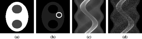
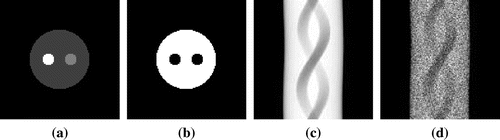
Fig. 2 (a) Attenuation map $a=a(x)$, (b) emiter activity $f=f(x)$, (c) noiseless emission data $g=P_{W}f(\mathit{\gamma })$, (d) noisy emission data $p=p(\mathit{\gamma })$ (30% noise) for phantom 2. (See Subsections 3.1, 3.3)

Phantom 1 is a version of the elliptical chest phantom (used for the numerical simulations of cardiac SPECT imaging; see e.g. [16, 21, 22]). Actually, this version is the same as in [16, 22] and, in addition to Figure 1, its description includes the following information:

1. the major axis of the ellipse representing the body is 30 cm,

2. attenuation coefficient a is 0.04 cm${}^{-1}$ in the lung region (modelled as two interior ellipses), 0.15 cm${}^{-1}$ elsewhere within the body ellipse and zero outside the body,

3. emitter activity f is in the ratio 8:0:1:0 in myocardium (represented as a ring), lungs, elsewhere within the body and outside the body,

4. noisy emission data $p$ contain 30% of the Poisson noise in the sense of $L^2$-norm and the total number of photons is 125 450. Phantom 2 is a simulated numerical version of the Utah phantom (designed at the 2${}^{\mathit{nd}}$ International Meeting on fully Three-Dimensional Image Reconstruction in Radiology and Nuclear Medicine, Snowbird, Utah, 1993). A real non-simulated version of this phantom was considered, in particular, in [23]. However, in the present work we consider its simulated numerical version in order to see clearly different reconstruction errors. In addition to Figure 2, the description of phantom 2 includes the following information:

5. geometrically the phantom consists of a large disk containing two small disks, where the radius of the large disks is 10 cm,

6. attenuation coefficient a is 0.16 cm${}^{-1}$ in the large disk outside the small disks, 0.63 cm${}^{-1}$ in the left small disk, 0.31 cm${}^{-1}$ in the right small disk, and zero outside the large disk,

7. emitter activity f is a positive constant in the large disk outside the small disks and zero elsewhere

8. noisy emission data p contain 30% of the Poisson noise in the sense of $L^2$-norm and the total number of photons is 89 350.

Note also that all computations of the present work are fulfilled using the same numerical realizations of basic formulas as in [16, 22, 23].

Results for the bounds ${\mathit{\sigma }}_{W,D,m}$ and ${\mathit{\rho }}_{W,D,m}$

The bound numbers ${\mathit{\sigma }}_{W,D,m}$, ${\mathit{\rho }}_{W,D,m}$ of (2.11), (2.30) for phantoms 1 and 2 are shown in Tables 1 and 2, where $D={\mathcal{B}}_R$.

Table 1 Numbers ${\mathit{\sigma }}_{W,D,m}$, ${\mathit{\rho }}_{W,D,m}$ of (2.11), (2.30) for phantom 1, where $D={\mathcal{B}}_R$.

	$m=1$	$m=2$	$m=3$	$m=20$
${\mathit{\sigma }}_{W,D,m}$	0.390	0.584	0.739	1.320
${\mathit{\rho }}_{W,D,m}$	1.399	2.025	2.494	4.532

Table 2 Numbers ${\mathit{\sigma }}_{W,D,m}$, ${\mathit{\rho }}_{W,D,m}$ of (2.11), (2.30) for phantom 2, where $D={\mathcal{B}}_R$.

	$m=1$	$m=2$	$m=3$	$m=20$
${\mathit{\sigma }}_{W,D,m}$	0.489	0.694	0.803	1.296
${\mathit{\rho }}_{W,D,m}$	3.112	4.567	5.436	9.719

For phantoms 1 and 2, Tables 1 and 2 show that condition (2.19) with ${\mathit{\sigma }}_{\mathit{max}}$ = 0.7 is fulfilled for m = 1 and m = 2, whereas ${\mathit{\rho }}_{W,D,m}>1$ already for $m=1$.

Table 3 Relative reconstruction errors $\mathit{\eta }(f_m,f,X),\mathit{\eta }(f_m^{+},f,X)$ for the noiseless case for phantom 1.

	$m=0$	$m=1$	$m=2$	$m=3$	$m=20$
$\mathit{\eta }(f_m,f,X)$	0.331	0.305	0.295	0.293	0.288
$\mathit{\eta }(f_m^{+},f,X)$	0.331	0.305	0.295	0.293	0.287

 

Reconstruction results for the emitter activity f

For phantoms 1 and 2 we consider the approximate reconstructions $f_m$ realized numerically via (2.20b) (using the method of successive approximations i.e. using (2.16)) from the noiseless data g and filtered noisy data $\stackrel{\sim }{p}$. The method of successive approximations was always realized in the framework of 4 iterations. In addition:

1. we consider $f_m$, mainly, under the condition that ${\mathit{\sigma }}_{W,D,m}\le {\mathit{\sigma }}_{\max }=0.7$,

2. we consider $\stackrel{\sim }{p}=\mathcal{W}p$ for $\mathcal{W}={\mathcal{A}}_{8,8}^{\mathit{sym}}$, where $\mathcal{W}={\mathcal{A}}_{l_1,l_2}^{\mathit{sym}}$ is the approximately optimal space-variant Wiener-type filter of Section 5.3 of [22].

 

Table 4 Relative reconstruction errors $\mathit{\eta }(f_m,f,X),\mathit{\eta }(f_m^{+},f,X)$ for the noiseless case for phantom 2.

	$m=0$	$m=1$	$m=2$	$m=3$	$m=20$
$\mathit{\eta }(f_m,f,X)$	0.292	0.179	0.152	0.141	0.137
$\mathit{\eta }(f_m^{+},f,X)$	0.168	0.151	0.138	0.136	0.137

In addition to $f_m$ we consider also their non-negative parts $f_m^{+}$, where$$f_m^{+}(x)=f_m(x)\mathrm{if}{f}_m(x)\ge 0\mathrm{and}{f}_m^{+}(x)=0\mathrm{if}{f}_m(x)<0$$For phantoms 1 and 2, Tables 1 and 2 show that ${\mathit{\sigma }}_{W,D,m}\le 0.7$ is fulfilled for $m=0,1,2$ only.

To study reconstruction errors we consider, in particular,(3.3) $$\begin{array}{c}\hfill \begin{array}{c}\mathit{\eta }(u_2,u_1,X)=\frac{\parallel u_2-u_1{\parallel }_{L^2(X)}}{\parallel u_1{\parallel }_{L^2(X)}},\hfill \end{array}\end{array}$$(3.3) where $u_1$, $u_2$ are test functions on X.

The approximate reconstructions $f_0$, $f_2$ with their central horizontal profiles from the noiseless data g for phantoms 1 and 2 are shown in Figures 3 and 4.

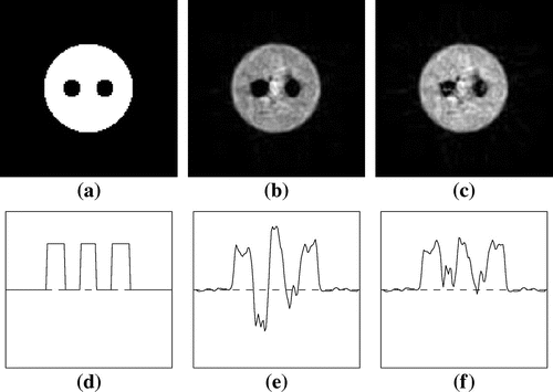
Fig. 3 Phantom 1:(a) true f, (b), (c) approximate reconstructions $f_0$, $f_2$ from the noiseless data g, (d), (e), (f) central horizontal profiles. (See Subsections 3.3, 3.5)

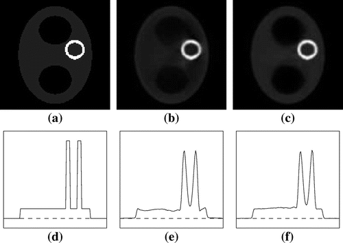
Fig. 4 Phantom 2:(a) true f, (b), (c) approximate reconstructions $f_0$, $f_2$ from the noiseless data g, (d), (e), (f) central horizontal profiles. (See Subsections 3.3, 3.5)

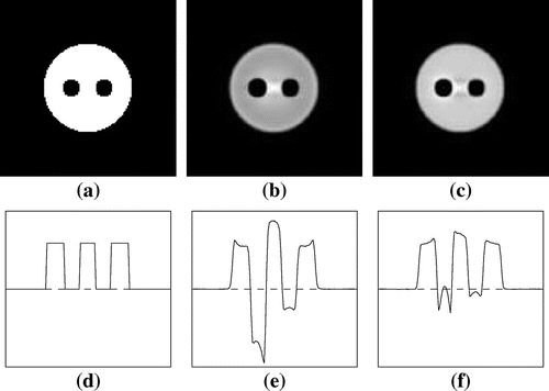
Fig. 5 Phantom 1: (a) true f, (b), (c) approximate reconstructions $f_0$, $f_2$ from the filtered noisy data $\stackrel{\sim }{p}={\mathcal{A}}_{8,8}^{\mathit{sym}}p$ (30% noise), (d), (e), (f) central horizontal profiles. (See Subsections 3.3, 3.5)

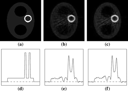
Fig. 6 Phantom 2: (a) true f, (b), (c) approximate reconstructions $f_0$, $f_2$ from the filtered noisy data $\stackrel{\sim }{p}={\mathcal{A}}_{8,8}^{\mathit{sym}}p$ (30% noise), (d), (e), (f) central horizontal profiles. (See Subsections 3.3, 3.5)

Tables 3 and 4 show the relative errors $\mathit{\eta }(f_m,f,X)$ and $\mathit{\eta }(f_m^{+},f,X)$ in $L^2$- norm for the approximate reconstructions $f_m$ with respect to precise f for the noiseless case for phantoms 1 and 2.

Table 5 Relative errors $\mathit{\eta }(f_m,f,X),\mathit{\eta }(f_m^{+},f,X)$ for $f_m$ reconstructed from $\stackrel{\sim }{p}={\mathcal{A}}_{8,8}^{\mathit{sym}}p$ for phantom 1.

	$m=0$	$m=1$	$m=2$	$m=3$	$m=20$
$\mathit{\eta }(f_m,f,X)$	0.398	0.380	0.374	0.373	0.368
$\mathit{\eta }(f_m^{+},f,X)$	0.398	0.379	0.373	0.371	0.366

Table 6 Relative errors $\mathit{\eta }(f_m,f,X),\mathit{\eta }(f_m^{+},f,X)$ for $f_m$ reconstructed from $\stackrel{\sim }{p}={\mathcal{A}}_{8,8}^{\mathit{sym}}p$ for phantom 2.

	$m=0$	$m=1$	$m=2$	$m=3$	$m=20$
$\mathit{\eta }(f_m,f,X)$	0.268	0.218	0.218	0.225	0.248
$\mathit{\eta }(f_m^{+},f,X)$	0.214	0.209	0.213	0.221	0.245

Figures 3, 4 and Tables 3, 4 show that for phantoms 1 and 2 for the noiseless case the approximations $f_1$, $f_2$ are considerably more precise than the classical Chang approximation $f_0$.

In particular, for phantom 2 for the noiseless case $f_2$ is drastically more precise than $f_0$ if we take also into account their negative parts!

The approximate reconstructions $f_0$, $f_2$ with their central horizontal profiles from the filtered noisy data $\stackrel{\sim }{p}={\mathcal{A}}_{8,8}^{\mathit{sym}}p$ for phantoms 1 and 2 are shown in Figures 5 and 6, where ${\mathcal{A}}_{l_1,l_2}^{\mathit{sym}}$ is the aforementioned filter of [22].

Tables 5 and 6 show the relative errors $\mathit{\eta }(f_m,f,X)$ and $\mathit{\eta }(f_m^{+},f,X)$ in $L^2$- norm for $f_m$ reconstructed from filtered noisy data $\stackrel{\sim }{p}={\mathcal{A}}_{8,8}^{\mathit{sym}}p$ for phantoms 1 and 2.

Figures 5, 6 and Tables 5, 6 show that for phantoms 1 and 2 for the noisy case the approximations $f_1$, $f_2$ are also more correct than the classical Chang approximation $f_0$.

In particular, for phantom 2 for the noisy case $f_1$, $f_2$ are considerably more precise than $f_0$ if we take also into account their negative parts.

Table 6 also shows that the reconstruction quality of $f_m$ may degrade for large m. However, this degradation is absent in other numerical examples of this work. Apparently, this can be explained by the fact that our bounds ${\mathit{\sigma }}_{W,D,m}$ remain relatively small for large m in our numerical examples, see Tables 1 and 2.

Conclusions

In this work, we showed that the classical Chang approximate inversion formula (1.6) admits a very natural extention into inversion via finite Fourier series weight approximations or, more precisely, into inversion via (2.20) considered under assumption (2.19). Related theoretical considerations are presented in Sections 1 and 2 and numerical examples in the framework of SPECT are given in Section 3. Our examples of Section 3 include comparisons with the approximate Chang reconstruction $f_0$ and show numerical efficiency (with respect to precision and stability) of our approximate reconstructions $f_m$ for $m>0$, under the condition that inequality (2.19) is fulfilled (with ${\mathit{\sigma }}_{\mathit{max}}$ = 0.7 in our examples), see Figures 3–6 and Tables 3–6. In addition, possible advantages of our $f_m$ for $m>0$ in comparison with $f_0$ are especially obvious from Figures 4(d)–(f) and 6(d)–(f). Besides, Tables 5 and 6 show that our errors compare well with the 30% noise in the data.

Note also that considerations of Subsections 2.5 and 3.4 explain convergence of the iterative inversion of [2] for many cases when the inequality of (2.30) is not fulfilled. The point is that less restrictive inequality (2.27) is sufficient for this convergence.

Acknowledgments

The authors are grateful to M.V. Klibanov and to anonymous referees for remarks that have helped to improve the presentation. The second author was partially supported by TFP No 14.A18.21.0866 of Ministry of Education and Science of Russian Federation (at Faculty of Control and Applied Mathematics of Moscow Institute of Physics and Technology).

References

- Natterer F. The mathematics of computerized tomography. Stuttgart: Teubner; 1986.
- Kunyansky LA. Generalized and attenuated Radon transforms:restorative approach to the numerical inversion. Inverse Probl. 1992;8:809–819.
- Quinto ET. The invertibility of rotation invariant Radon transforms. J. Math. Anal. Appl. 1983;91:510–522.
- Miqueles EX, De Pierro AR. Fluorescence tomography:reconstruction by iterative methods, ISBI. 2008;8:760–763.
- Bal G. Inverse transport theory and applications, Inverse Probl. 2009;25:053001 (48pp).
- Radon J. Uber die Bestimmung von Funktionen durch ihre Integralwerte langs gewisser Mannigfaltigkeiten. Ber. Verh. Sachs. Akad. Wiss. Leipzig, Math-Nat. 1917;K 1 69:262–267.
- Novikov RG. An inversion formula for the attenuated X-ray transformation. Ark. Mat. 2002;40:145–167.
- Tretiak OJ, Metz C. The exponential Radon transform. SIAM J. Appl. Math. 1980;39:341–354.
- Boman J, Strömberg JO. Novikov’s inversion formula for the attenuated Radon transform - a new approach. J. Geom. Anal. 2004;14:185–198.
- Gindikin S. A remark on the weighted Radon transform on the plane. Inverse Probl. Imag. 2010;4:649–653.
- Novikov RG. Weighted Radon transforms for which Chang’s approximate inversion formula is exact. Uspekhi Mat. Nauk. 2011;66(2):237–238.
- Arbuzov EV, Bukhgeim AL, Kazantsev SG. Two-dimensional tomography problems and the theory of A-analytic functions. Siberian Adv. Math. 1998;8(4):1–20.
- Boman J. An example of non-uniqueness for a generalized Radon transform. J. Anal. Math. 1993;61:395–401.
- Boman J, Quinto ET. Support theorems for real-analytic Radon transforms. Duke Math. J. 1987;55:943–948.
- Chang LT. A method for attenuation correction in radionuclide computed tomography. IEEE Trans. Nucl. Sci. 1978;NS–25:638–643.
- Guillement J-P, Novikov RG. Optimized analytic reconstruction for SPECT. J. Inv. Ill-Posed Problems. 2012;20:489–500.
- Novikov RG. Weighted Radon transforms and first order differential systems on the plane, Available from: http://hal.archives-ouvertes.fr/hal-00714524.
- Beilina L, Klibanov MV. The philosophy of the approximate global convergence for multidimensional coefficient inverse problems. Complex Var. and Ellip. Equa. 2012;57(2–4):277–299.
- Beilina L, Klibanov MV. Approximate global convergence and adaptivity for coefficient inverse problems. New York: Springer; 2012.
- Vekua IN. Generalized analytic functions. London: Pergamon Press; 1962.
- Bronnikov AV. Reconstruction of the attenuation map using discrete consistency conditions. IEEE Trans. Med. Imaging. 2000;19:451–462.
- Guillement J-P, Novikov RG. On Wiener type filters in SPECT. Inverse Probl. 2008;24:025001.
- Guillement J-P, Jauberteau F, Kunyansky L, Novikov R, Trebossen R. On single-photon emission computed tomography imaging based on an exact formula for the nonuniform attenuation correction. Inverse Probl. 2002;18:L11–L19.