Determination of space–time-dependent heat source in a parabolic inverse problem via the Ritz–Galerkin technique

Abstract

Three inverse problems of reconstructing the time-dependent, spacewise- dependent and both initial condition and spacewise-dependent heat source in the one-dimensional heat equation are considered. These problems are reformulated by eliminating the unknown functions using some special assumptions concerning the points in space or time as additional measurements. Then direct techniques are proposed to solve the non-classical boundary value problems. For obtaining the robust and stable approximations, Bernstein multi-scaling and B-spline basis functions in the context of the Ritz–Galerkin method are utilized to immediate passage from differential equations to algebraic equations and afterwards, a Newton-type method is used to produce the admissible solution. The numerical convergence and stability are discussed in the test examples to show that the presented schemes provide accurate and acceptable approximations.

Keywords:

• parabolic equation
• inverse problem
• Ritz–Galerkin method
• heat source

AMS Subject Classifications:

• 35K05
• 35K20
• 65M32
• 65N35
• 65Z05

1 Introduction

The core of applied mathematical models is made up of partial differential equations.[1] These models can be divided into two general classifications as direct and inverse problems. Today, the literature on both analytical and numerical methods for the solution of direct problems, even for multidimensional cases, is well extended. While for the inverse problems, this matter still remains poorly developed. Inverse problems in physics often belong to the class of ill-posed problems. Mathematically speaking, in these problems, apart from the both issues of existence and uniqueness of the solution that appear extremely difficult to be shown, there is also the issue of stability to deal with, i.e. the continuous dependence of the solution on input data.[2] The key note in the approximate solution of the inverse problems is the requirement to identify the right-hand side, leading coefficients and parameters, and some initial and boundary conditions of time-dependent or stationary equations. On the other hand, since a wide area of the sciences and engineering phenomena are modelled by these problems, the main intent is to draw attention to the use of more applicable and accurate algorithms that makes it possible to determine the unknown function using some given observation at accessible parts of the domain of the problem. Producing more accurate methods for inverse problems rests on the development and examination of numerical methods for boundary value problems formulated for basic equations in mathematical physics.[1] On top of that, in the past few decades, a great deal of interest has been directed towards the determination of unknown coefficients which represent physical quantities, for example, the conductivity of a medium, in second-order equations, especially to parabolic equations. As an example for application of inverse problems in modelling the stationary equations, we can point to the process of reconstructing the mass distribution in the problems of potential theory formulated by Laplace equation, if a mass distribution is not known but its potential outside a certain ball is given and the goal is finding this mass distribution.[3] Besides, inverse boundary value problems can be used in modelling the diffusion processes like denoting the concentration of a chemical or temperature in the context of the heat conduction problems.[4, 5] Also for determination of source parameter in the wave equation, we refer the interested reader to [6].

1.1 The main aim of the current paper

Here, what will be pursued is retrieving the right-hand side (RHS) term of the parabolic equations. Also a particular attention has been focused on both cases i.e. dependence of the RHS on time and space as the unknown variables. In the theory of inverse problems of heat transfer,[7–9] among other problems there are problems of reconstructing unknown heat sources on the basis of measurements of the temperature at particular points.

1.2 Some applications

Some important applied problems of hydrogeology and the process of diffusion and conduction of natural materials or in the mass transfer are formulated in a similar way.[10, 11] Paying attention to the importance of the right-hand side identification of the parabolic equations becomes more justifiable when we realize the application of these mathematical problems in modelling the influences of the disasters induced by human activities, known as the environmental problems. These difficulties especially include soil and groundwater contamination, release of chemical, biological or nuclear agents to the atmosphere, release of pollutants to the aquatic systems like oil spills and contamination of some areas of the earth caused by release of large amounts of radioactive isotopes.[12] All of the mentioned cases have encountered to our life environment and severely treated it especially over last 30 years. As the clear example we can take into account the accident occurred at the Chernobyl nuclear power plant in northern Ukraine in 1986 and the oil spill that occurred in 1979 in the gulf of Mexico.

Nowadays, the concern about the reciprocal effects of both human and nature to the environment is increasing. At the first step, it seems absolutely necessary to provide accurate and appropriate formulas that comprehensively model these environmental phenomena to minimize the influences of the disasters. However this fact is very complicated and cannot be completely achieved. The next step is presenting the analytical or numerical techniques to find the accurate and stable solution to realize and predict the amount of the effects on the environment. As a general formulation that models describing the processes of heat, moisture, radiation, and pollutants transport and transformation in the atmosphere, we can state [12]$$\begin{array}{c}\hfill L\mathcal{A}=0,\mathrm{in}{D}_t=D\times (0,t),\end{array}$$where$$\begin{array}{cc}\hfill L\mathcal{A}& \equiv \frac{\mathit{\partial }\mathit{\pi }{\mathcal{A}}_i(\mathbf{x},t)}{\mathit{\partial }t}+div\mathit{\pi }({\mathcal{A}}_i(\mathbf{x},t)u-{\mathit{\mu }}_{i}grad{\mathcal{A}}_i(\mathbf{x},t))\hfill \\ & +\mathit{\pi }({(H\mathcal{A}(\mathbf{x},t))}_i-f_i(\mathbf{x},t)-r_i),i=\overline{1,n}.\hfill \end{array}$$Here ${\{{\mathcal{A}}_i(\mathbf{x},t)\}}_{i=\overline{1,n}}$ are the potential temperature, the mixing ratio of humidity in the atmosphere (water vapour, cloud water, rain water, snow and ice crystals), the concentration of pollutants in gas and aerosol phase); ${\{f_i(\mathbf{x},t)\}}_{i=\overline{1,n}}$ is the function of heat, moisture and pollutants sources; ${\{r_i\}}_{i=\overline{1,n}}$ are the functions describing uncertainty and errors of the models; $u=(u_1,u_2,u_3)$ is the velocity vector; $\mathit{\pi }$ is the function depending on the coordinate system; $\mathit{\mu }=({\mathit{\mu }}_1,{\mathit{\mu }}_2,{\mathit{\mu }}_3)$ are the coefficients of turbulent exchange for a substance ${\mathcal{A}}_i$ in the coordinate direction $\mathbf{x}=(x_1,x_2,x_3)$; $H\mathcal{A}$ is the non-linear matrix operator which describes the local processes of transformation of the corresponding substances. The initial condition, the boundary conditions and the model parameters can be written in the form:$$\begin{array}{c}\hfill {\mathcal{A}}^0={\mathcal{A}}_a^0+\mathit{\zeta }(\mathbf{x}),{(R_b\mathcal{A})}_i-g_i={\mathit{\varrho }}_i,i=\overline{1,n},Y=Y_a+\mathit{\xi }(\mathbf{x},t),\end{array}$$where ${\mathcal{A}}_a^0$ and $Y_a$ are the set of the prior estimations of the initial fields ${\mathcal{A}}^0$ and the vector of parameters, $Y,\mathit{\zeta }(\mathbf{x}),\mathit{\xi }(\mathbf{x},t)$ are the errors and uncertainty of initial fields and parameters; $R_b$ are the operators of boundary conditions, and $g_i,{\mathit{\varrho }}_i$ are functions describing sources and uncertainty at the boundary $D_t$. The extra observation for the inverse problem can be considered as$$\begin{array}{c}\hfill {\mathrm{\Sigma }}_m={[W\mathcal{A}]}_m+\mathrm{{\rm Y}}(\mathbf{x},t),\end{array}$$where ${\mathrm{\Sigma }}_m$ is the set of measured values; ${[W\mathcal{A}]}_m$ is the set of observational models; $\mathrm{{\rm Y}}(\mathbf{x},t)$ are the errors and uncertainty of these models and data. The values ${\mathrm{\Sigma }}_m$ are defined on the set of points $D_t^m\in D_t$. The symbol ${[·]}_m$ denotes the operation of data transfer from $D_t$ to $D_t^m$. For more background on the model, we refer the interested reader to [12] and the references therein.

1.3 Literature review

For the case of reconstructing the time-dependent heat source, the traditional approach in solving problems of source identification approximately consists in reduction of the inverse problem to the Volterra integral equation of the first kind using the Green function,[13] and in [14, 15] authors have investigated some methods for identification problems that the output of a dynamic system is used to reconstruct the unknown input actions on the system. Borukhov and Vabishchevich [10] presented a numerical algorithm based on the transition to the problem of the loaded parabolic equation and applied a difference scheme to solve the non-classical problem. Moreover, in [16] a numerical algorithm on the basis of the Landweber iteration is designed to deal with the problem. For the case of recovering the spacewise-dependent heat source, the theoretical and numerical methods are presented by several authors.[17–28] The numerical schemes include the finite difference method,[20] the radial basis functions method,[29] the boundary elements method,[19] the combination of the boundary elements method and variational method,[23–26] a simplified Tikhonov regularization method.[18]

Also see [30–32].

Here, we extend the Ritz–Galerkin method for solving such inverse problems of determination of the unknown heat sources from the standard overspecified boundary data.

1.4 The structure of this paper

The structure of this article is as follows:

In Section 2, the inverse problems with the essential conditions for the existence and uniqueness of the solution are presented. Section 3 is dedicated to introduce the basis functions which will be used in the sequel. Section 4 states the numerical schedules to solve the inverse problems. Finally, the numerical experiments will become apparent in Section 5 to testify the presented algorithm with some benchmark test examples. Section 6 consists of a brief summary.

2 Problem statement

2.1 The first inverse problem (IP1)

Assume that the state of the problem is governed by the following equation:1 $$\begin{array}{c}\hfill \frac{\mathit{\partial }A}{\mathit{\partial }t}-\frac{\mathit{\partial }}{\mathit{\partial }x}\left(k,(x),\frac{\mathit{\partial }A}{\mathit{\partial }x}\right)=f(x,t)\mathrm{in}Q=\mathrm{\Omega }\times (0,T],\end{array}$$1 where $k(x)$ is smooth enough positive coefficient and the problem is supplemented with two boundary conditions given at the end points of the segment $[0,1]$2 $$\begin{array}{c}\hfill A(0,t)=A(1,t)=0,t\in [0,T],\end{array}$$2 the initial condition is also prescribed3 $$\begin{array}{c}\hfill A(x,0)=A_0(x),0<x<1.\end{array}$$3 The inverse problem of recovering the unknown functions $\{A(x,t),f(x,t)\}$ is considered as IP1 along with the additional condition4 $$\begin{array}{c}\hfill A(x^{\ast },t)=\mathit{\phi }(t),x^{\ast }\in (0,1).\end{array}$$4 We suppose that the function $f(x,t)$ can be represented as5 $$\begin{array}{c}\hfill f(x,t)=\mathit{\delta }(x)\mathit{\sigma }(t),\end{array}$$5 where $\mathit{\delta }(x)$ is the given function and the time-dependent function $\mathit{\sigma }(t)$ is aimed to be approximated. Problems concerning the unique solution for this class of inverse problems for parabolic equations are reviewed in [16, 33]. We consider the following compatibility conditions and restrictions for obtaining the solution of this problem:

(1)	$\mathit{\delta }(x^{\ast })\ne 0$,
(2)	$\mathit{\delta }(x)$ is a sufficiently smooth function ($\mathit{\delta }\in C^2[0,1]$),
(3)	$\mathit{\delta }(x)=0$ on the boundary of the calculation domain,
(4)	$A_0(0)=A_0(1)=0,A_0(x^{\ast })=\mathit{\phi }(0)$.

2.2 The second inverse problem (IP2)

Often in melting and freezing processes, a possible way of designing final states is by controlling initial data and heat sources.[26] For the presentation of the problem, generally we consider a non-homogeneous and non-isotropic body, denoted by $\mathrm{\Omega }$, occupying a bounded domain in ${\mathbb{R}}^{n\ge 1}$ and strive to approximate both quantities of the initial condition and heat source $\{\mathit{\phi }(x),f(x)\}$ in the following heat equation i.e. Equation (66 $$\begin{array}{c}\hfill \left\{\begin{array}{cc}{\mathit{\partial }}_{t}A+LA=f(x),\hfill & \mathrm{in}\mathrm{\Omega }\times (0,T),\hfill \\ A=0,\hfill & \mathrm{on}\mathrm{\Gamma }\times (0,T),\hfill \\ A(x,0)=\mathit{\phi }(x),\hfill & x\in \mathrm{\Omega },\hfill \end{array}\right.\end{array}$$6 ). In the present work, the insufficiency of the input information is compensated by considering some additional information at two different instants of time $T_2>T_1>0$. As a mathematical model, we suppose that the process satisfies the following parabolic equation:6 $$\begin{array}{c}\hfill \left\{\begin{array}{cc}{\mathit{\partial }}_{t}A+LA=f(x),\hfill & \mathrm{in}\mathrm{\Omega }\times (0,T),\hfill \\ A=0,\hfill & \mathrm{on}\mathrm{\Gamma }\times (0,T),\hfill \\ A(x,0)=\mathit{\phi }(x),\hfill & x\in \mathrm{\Omega },\hfill \end{array}\right.\end{array}$$6 along with the additional observations:7 $$\begin{array}{c}\hfill A(x,T_1)={\mathit{\psi }}_1(x),A(x,T_2)={\mathit{\psi }}_2(x).\end{array}$$7 Here we assume that L belongs to the class of the linear elliptic operators of second order, for simplicity, time-independent smooth coefficients, presented as $L=-\nabla .[k(x)\nabla ]$ where $k>0$ is the thermal conductivity, $\mathrm{\Gamma }=\mathit{\partial }\mathrm{\Omega }$ and $T_2\le T$. For this problem, the results of existence and uniqueness of the solution are given in [26]. For the uniqueness we have the following theorem

Theorem 2.1

Let ${\mathit{\psi }}_1,{\mathit{\psi }}_2\in H_0^1(\mathrm{\Omega })\cap H^2(\mathrm{\Omega })$. Then the inverse problem (66 $$\begin{array}{c}\hfill \left\{\begin{array}{cc}{\mathit{\partial }}_{t}A+LA=f(x),\hfill & \mathrm{in}\mathrm{\Omega }\times (0,T),\hfill \\ A=0,\hfill & \mathrm{on}\mathrm{\Gamma }\times (0,T),\hfill \\ A(x,0)=\mathit{\phi }(x),\hfill & x\in \mathrm{\Omega },\hfill \end{array}\right.\end{array}$$6 )–(77 $$\begin{array}{c}\hfill A(x,T_1)={\mathit{\psi }}_1(x),A(x,T_2)={\mathit{\psi }}_2(x).\end{array}$$7 ) has a unique solution among initial conditions $\mathit{\phi }\in H_0^1(\mathrm{\Omega })\cap H^2(\mathrm{\Omega })$, sources $f\in L^2(\mathrm{\Omega })$ and temperature $A$ that satisfy$${\int }_{[0,T]}\left\{\Vert ,A_t,{(·,t)\Vert }_{L^2(\mathrm{\Omega })}^2,+,{\Vert A(·,t)\Vert }_{H^2(\mathrm{\Omega })}^2\right\}dt<\infty .$$It is possible to extend this result to a weaker assumption on the data but one then has to consider an appropriate weak formulation of (66 $$\begin{array}{c}\hfill \left\{\begin{array}{cc}{\mathit{\partial }}_{t}A+LA=f(x),\hfill & \mathrm{in}\mathrm{\Omega }\times (0,T),\hfill \\ A=0,\hfill & \mathrm{on}\mathrm{\Gamma }\times (0,T),\hfill \\ A(x,0)=\mathit{\phi }(x),\hfill & x\in \mathrm{\Omega },\hfill \end{array}\right.\end{array}$$6 ) and (77 $$\begin{array}{c}\hfill A(x,T_1)={\mathit{\psi }}_1(x),A(x,T_2)={\mathit{\psi }}_2(x).\end{array}$$7 ). As more clarifications, related to this problem, we can point to the two of the most important problems and respectively belong to the two general classes, evolutionary inverse problems and boundary value inverse problems which model the classic ice melting and metal solidification, crystal growth, casting, welding, melting, ablation, etc. where the heat sources are supposed to be absent.[34] The problems are well known as the Cauchy–Stefan and Stefan problems which originally treat the formation of ice in the polar seas. They named after the Slovene physicist, Jozef Stefan who introduced the general class of such problems and it can appear in several formulations.[35–40]

2.3 The third inverse problem (IP3)

Following the inverse source problem of determining a pair of functions $\{A(x,t),S(x,t)\}$ satisfying the equation8 $$\begin{array}{c}\hfill \mathit{\rho }(x,t)A_t-\mathrm{\Delta }A=S(x,t),\mathrm{in}\mathrm{\Omega }\times [0,T],\end{array}$$8 supplemented with the initial condition9 $$\begin{array}{c}\hfill A(x,0)=A_0(x),x\in \mathrm{\Omega },\end{array}$$9 and the boundary condition10 $$\begin{array}{c}\hfill A(x,t)=s(t),x\in \mathit{\partial }\mathrm{\Omega },0\le t\le T,\end{array}$$10 and the extra specification is11 $$\begin{array}{c}\hfill A(x,T)=r(x),x\in \mathrm{\Omega },\end{array}$$11 where $S(x,t)=f(x)g(x,t)+h(x,t)$ that $h(x,t),g(x,t)$ are two known functions, $f(x)$ is unknown in its domain and $\mathrm{\Omega }$ is a bounded domain in ${\mathbb{R}}^n$ with smooth boundary $\mathit{\partial }\mathrm{\Omega }$. In the modelling of air pollution phenomena, $S(x,t)$ is assumed as the source pollutant. Thus, an accurate estimation of the pollutant source is crucial to environmental safeguard in cities with high populations, see [11, 18]. Considering the boundary condition (1010 $$\begin{array}{c}\hfill A(x,t)=s(t),x\in \mathit{\partial }\mathrm{\Omega },0\le t\le T,\end{array}$$10 ) as12 $$\begin{array}{c}\hfill A(0,t)=\mathit{\phi }(t),A(1,t)=\mathit{\psi }(t),0\le t\le T,\end{array}$$12 and $Q=\{(x,t)\mid (x,t)\in [0,1]\times [0,T]\}$, the following theorem guarantees the unique solvability of this problem.[41]

Theorem 2.2

Under the assumptions (A1)–(A5), the IP3 possesses a unique solution.$$(\mathrm{A}1):\mathrm{\Lambda }1\le \mathit{\rho }(x,t)\le {\mathrm{\Lambda }}_2,-K_{\mathit{\rho },1}\le {\mathit{\rho }}_t(x,t)\le K_{\mathit{\rho },2},(x,t)\in \overline{Q},$$$$(\mathrm{A}2):\mid g(x,t)\mid \le K_g,\mid g_t(x,t)\mid \le K_g^{\ast },\mid g_t(x,t)\mid \ge g_0>0,(x,t)\in \overline{Q},$$$$(\mathrm{A}3):h(x,t)\in C(0,T;L^2(\mathrm{\Omega })),\Vert h(·,t)\Vert \le K_h,h_t(x,t)\in L^2(Q),{\Vert A\Vert }_{L^2(Q)}\le K_h,$$$$(\mathrm{A}4):A_0(x)\in W_2^2(\mathrm{\Omega })\cap W_2^{1^{\circ }},{\Vert A_0\Vert }_{W_2^2(\mathrm{\Omega })}\le M_h,$$$$(\mathrm{A}5):f(x)\in W_2^2(\mathrm{\Omega })\cap W_2^{1^{\circ }},{\Vert f\Vert }_{W_2^2(\mathrm{\Omega })}\le K_{\mathit{\phi }},$$where ${\mathrm{\Lambda }}_1,{\mathrm{\Lambda }}_2,K_g,g_0$ are positive constants, $K_{\mathit{\rho },1},K_{\mathit{\rho },2},K_g^{\ast },K_h,M_0,K_{\mathit{\phi }}$ are non-negative constants, and the spaces $L^2(Q),L^2(\mathrm{\Omega }),W_2^2(\mathrm{\Omega }),W_2^{1^{\circ }},C(0,T;L^2(\mathrm{\Omega }))$ with the corresponding norms are used in the usual sense.[11, 41, 42]

3 Basis functions

3.1 Properties of the B-spline functions

In order to construct the approximate solution for the unknown function $A(\mathit{\eta },\mathit{\xi })$ defined over $[a,b]\times [c,d]$, we utilize the finite expansions in terms of the B-spline scaling functions. Since these basis functions are defined on the the interval $[0,1]$, at first we map the finite intervals $[a,b],[c,d]$ to the interval [0,1]. Thus, we employ the affine transformations [43]:$$\mathit{\eta }=(b-a)x+a,0\le x\le 1,$$$$\mathit{\xi }=(d-c)t+c,0\le t\le 1.$$Let $s$ and $t$ be positive integers, the interval $[\mathit{\alpha },\mathit{\beta }]$ is divided into t equal parts by a set of knots:$$\mathit{\alpha }=x_{-s+1}=...=x_0<x_1<...<x_t=...=x_{s+t-1}=\mathit{\beta },$$while the left and right end knots have [44] the multiplicity $s$. Cardinal B-spline functions of order $s\ge 2$ for the knots sequence $X={\{x_i\}}_{i=-s+1}^{s+t-1}$ can be computed as [45, 46]:$$B_{s,k,X}(x)=\frac{x-x_k}{x_{k+s-1}-x_k}{B}_{s-1,k,X}(x)+\frac{x_{k+s}-x}{x_{k+s}-x_{k+1}}{B}_{s-1,k+1,X}(x),$$$$k=-s+1,...,t-1,$$and$$B_{1,k,X}(x)=\left\{\begin{array}{cc}1,\hfill & x_k\le x\le x_{k+1},\hfill \\ 0,\hfill & \mathrm{otherwise},\hfill \end{array}\right.k=0,1,...,t-1.$$By considering the interval $[\mathit{\alpha },\mathit{\beta }]\equiv [0,1]$, at any level $j\in \mathbf{Z}$, the discretization step is $2^{-j}$, and this generates $t=2^j$ number of segments in [0,1] with knots sequence [47]$$x^{(j)}=\left\{\begin{array}{c}{x}_{-s+1}^{(j)}=...=x_0^{(j)}=0,\hfill \\ x_k=\frac{k}{2^j},k=1,...,2^j-1,\hfill \\ x_t^{(j)}=...=x_{s+t-1}^{(j)}=1.\hfill \end{array}\right.$$Let $j_0$ be the level for which $2^{j_0}\ge m$; for each level $j\ge j_0$ the scaling functions of order $m$ can be defined as follow [47]:$${\mathit{\varphi }}_{m,k}^{(j)}(x)=\left\{\begin{array}{cc}{B}_{m,k,X^{(j)}}(2^{j-j_0}x),\hfill & k=-m+1,...,-1,\hfill \\ B_{m,2^j-m-k,X^{(j)}}(1-2^{j-j_0}x),\hfill & k=2^j-m+1,...,2^j-1,\hfill \\ B_{m,0,X^{(j)}}(2^{j-j_0}x-2^{-j_0}k),\hfill & k=0,...,2^j-m.\hfill \end{array}\right.$$The scaling functions ${\mathit{\varphi }}_{m,k}^{(j)}(x)$ occupy m segments, therefore the condition $2^j\ge s$ must be satisfied in order to have at least one inner scaling function. The scaling functions used in this paper are linear, quadratic and cubic B-spline scaling functions, i.e. ${\mathit{\varphi }}_{m,k}^{(j)}(x)$, with $m=2,3,4$, respectively.

3.2 Properties of Bernstein multi-scaling functions

Bernstein multi-scaling functions ${\mathit{\psi }}_{i,n}(t)=B_{i,m}(\frac{k}{t_f}t-n)$ have four arguments [2, 48]:

(1)	Translation argument $n=0,1,\cdots ,k-1,$
(2)	Argument $k\ge 1$ which can assume any positive integer,
(3)	$m$ as the order of Bernstein polynomial on $[a,b],$
(4)	$t$, the normalized time,
(5)	They are defined on the interval $[0,t_f)$ as13 $$\begin{array}{c}\hfill {\mathit{\psi }}_{i,n}(t)=\left\{\begin{array}{cc}{B}_{i,m}(\frac{k}{t_f}t-n),\hfill & \frac{n{t}_f}{k}\le t<\frac{(n+1)t_f}{k},\hfill \\ 0,\hfill & \mathrm{otherwise}.\hfill \end{array}\right.\end{array}$$13 Also the $n$-dimensional Bernstein multi-scaling functions are defined as:14 $$\begin{array}{c}\hfill {\mathit{\psi }}_{i,n}(X)=\left\{\begin{array}{cc}\prod _{j=1}^M{B}_{i_j,m_j}\left(\frac{k_j}{x_{f_j}},x_j,-,n_j\right),\hfill & \frac{n_j{x}_{f_j}}{k_j}\le x_j<\frac{(n_j+1)x_{f_j}}{k_j},\hfill \\ 0,\hfill & \mathrm{otherwise},\hfill \end{array}\right.\end{array}$$14 where $X=(x_1,x_2,...,x_M),i=(i_1,i_2,...,i_M),n=(n_1,n_2,...,n_M),$$k_j$ is positive integer, $x_{f_j}$ is the endpoint of each interval that $x_j$ belongs to, $m_j$ is the order of Bernstein polynomial $B_{i,m}(x)$ defined by:15 $$\begin{array}{c}\hfill B_{i,m}(x)=\left(\genfrac{}{}{0pt}{}{m}{i}\right)\frac{{(x-a)}^i{(b-x)}^{m-i}}{{(b-a)}^m},0\le i\le m,\end{array}$$15 where$$\left(\genfrac{}{}{0pt}{}{m}{i}\right)=\frac{m!}{i!(m-i)!},$$on each interval $[a,b]$ and $i_j=0,1,...,m_j,$$n_j=0,1,...,k_j-1,j=1,2,...,M.$ The functions $\{{\mathit{\psi }}_{i,n}(X)\}$ form a basis for $L^2({\prod }_{j=1}^M[0,x_{f_j}])$, see [2, 48].
(6)	There are two degrees of freedom which increase the accuracy of the method. One of these parameters is the argument $k$ and another one is $m$ which corresponds to the degree of Bernstein polynomials in every subinterval $[\frac{n{t}_f}{k},\frac{(n+1)t_f}{k})$.
(7)	The upper bound of the error depends on $\sqrt{\frac{t_f}{2m+3}}\frac{1}{(m+1)!}{(\frac{t_f}{k})}^{m+1}$ which shows that the error reduces to zero very fast as $m$ and $k$ increase.[2, 48]

4 The solution procedure

4.1 The solution of IP1

Consider the following transformation [1, 10]:16 $$\begin{array}{c}\hfill \mathit{\varsigma }(t)={\int }_{[0,t]}\mathit{\sigma }(\mathit{\theta })d\mathit{\theta },\end{array}$$16 and set17 $$\begin{array}{c}\hfill A(x,t)=B(x,t)+\mathit{\delta }(x)\mathit{\varsigma }(t).\end{array}$$17 Substituting Equations (1616 $$\begin{array}{c}\hfill \mathit{\varsigma }(t)={\int }_{[0,t]}\mathit{\sigma }(\mathit{\theta })d\mathit{\theta },\end{array}$$16 ) and (1717 $$\begin{array}{c}\hfill A(x,t)=B(x,t)+\mathit{\delta }(x)\mathit{\varsigma }(t).\end{array}$$17 ) into (11 $$\begin{array}{c}\hfill \frac{\mathit{\partial }A}{\mathit{\partial }t}-\frac{\mathit{\partial }}{\mathit{\partial }x}\left(k,(x),\frac{\mathit{\partial }A}{\mathit{\partial }x}\right)=f(x,t)\mathrm{in}Q=\mathrm{\Omega }\times (0,T],\end{array}$$1 )–(55 $$\begin{array}{c}\hfill f(x,t)=\mathit{\delta }(x)\mathit{\sigma }(t),\end{array}$$5 ) and considering (44 $$\begin{array}{c}\hfill A(x^{\ast },t)=\mathit{\phi }(t),x^{\ast }\in (0,1).\end{array}$$4 ) we get the following representations [1, 10] for the unknown functions $\mathit{\varsigma }(t)$ and $B(x,t)$18 $$\begin{array}{c}\hfill \mathit{\varsigma }(t)=\frac{1}{\mathit{\delta }(x^{\ast })}\{\mathit{\phi }(t)-B(x^{\ast },t)\},\end{array}$$18 19 $$\begin{array}{c}\hfill \frac{\mathit{\partial }B}{\mathit{\partial }t}=\frac{\mathit{\partial }}{\mathit{\partial }x}\left\{k,(x),\frac{\mathit{\partial }B}{\mathit{\partial }x}\right\}+\frac{1}{\mathit{\delta }(x^{\ast })}\{\mathit{\phi }(t)-B(x^{\ast },t)\}\frac{\mathit{\partial }}{\mathit{\partial }x}\left\{k,(x),\frac{\mathit{\partial }\mathit{\delta }}{\mathit{\partial }x}\right\}.\end{array}$$19 Besides, for the initial and boundary conditions, due to the properties of (1616 $$\begin{array}{c}\hfill \mathit{\varsigma }(t)={\int }_{[0,t]}\mathit{\sigma }(\mathit{\theta })d\mathit{\theta },\end{array}$$16 ) and (1717 $$\begin{array}{c}\hfill A(x,t)=B(x,t)+\mathit{\delta }(x)\mathit{\varsigma }(t).\end{array}$$17 ), we have20 $$\begin{array}{c}\hfill B(x,0)=B_0(x),B(0,t)=B(1,t)=0,0<x<1,0\le t\le T.\end{array}$$20 Because of the term $B(x^{\ast },t)$, Equation (1919 $$\begin{array}{c}\hfill \frac{\mathit{\partial }B}{\mathit{\partial }t}=\frac{\mathit{\partial }}{\mathit{\partial }x}\left\{k,(x),\frac{\mathit{\partial }B}{\mathit{\partial }x}\right\}+\frac{1}{\mathit{\delta }(x^{\ast })}\{\mathit{\phi }(t)-B(x^{\ast },t)\}\frac{\mathit{\partial }}{\mathit{\partial }x}\left\{k,(x),\frac{\mathit{\partial }\mathit{\delta }}{\mathit{\partial }x}\right\}.\end{array}$$19 ) is non-classical. Now for reconstructing the Ritz-type approximation we use the following truncated series in terms of the basis functions21 $$\begin{array}{c}\hfill \overline{B(x,t)}=\sum _{n_1=0}^{k_1-1}\sum _{n_2=0}^{k_2-1}\sum _{i_1=0}^{m_1}\sum _{i_2=0}^{m_2}tx(x-1)c_{i_1,i_2,n_1,n_2}{\mathit{\psi }}_{i,n}(X)+B_0(x),\end{array}$$21 where $X=(x,t)$, ${\mathit{\psi }}_{i,n}(X)=B_{i_1,m_1}(k_{1}x-n_1)B_{i_2,m_2}\left(\frac{k_{2}t}{T},-,n_2\right)$ that was introduced in Section 3.2 and $B_0(x)=A_0(x)$. Due to the new compatibility condition22 $$\begin{array}{c}\hfill B_0(0)=B_0(1)=0,\end{array}$$22 induced from (2020 $$\begin{array}{c}\hfill B(x,0)=B_0(x),B(0,t)=B(1,t)=0,0<x<1,0\le t\le T.\end{array}$$20 ), the approximation (2121 $$\begin{array}{c}\hfill \overline{B(x,t)}=\sum _{n_1=0}^{k_1-1}\sum _{n_2=0}^{k_2-1}\sum _{i_1=0}^{m_1}\sum _{i_2=0}^{m_2}tx(x-1)c_{i_1,i_2,n_1,n_2}{\mathit{\psi }}_{i,n}(X)+B_0(x),\end{array}$$21 ) fulfils the initial and boundary conditions (2020 $$\begin{array}{c}\hfill B(x,0)=B_0(x),B(0,t)=B(1,t)=0,0<x<1,0\le t\le T.\end{array}$$20 ). Again we substitute (2121 $$\begin{array}{c}\hfill \overline{B(x,t)}=\sum _{n_1=0}^{k_1-1}\sum _{n_2=0}^{k_2-1}\sum _{i_1=0}^{m_1}\sum _{i_2=0}^{m_2}tx(x-1)c_{i_1,i_2,n_1,n_2}{\mathit{\psi }}_{i,n}(X)+B_0(x),\end{array}$$21 ) in (1919 $$\begin{array}{c}\hfill \frac{\mathit{\partial }B}{\mathit{\partial }t}=\frac{\mathit{\partial }}{\mathit{\partial }x}\left\{k,(x),\frac{\mathit{\partial }B}{\mathit{\partial }x}\right\}+\frac{1}{\mathit{\delta }(x^{\ast })}\{\mathit{\phi }(t)-B(x^{\ast },t)\}\frac{\mathit{\partial }}{\mathit{\partial }x}\left\{k,(x),\frac{\mathit{\partial }\mathit{\delta }}{\mathit{\partial }x}\right\}.\end{array}$$19 ) to obtain the residual function as [2, 49]23 $$\begin{array}{cc}\hfill Res(\overline{B(x,t)})& :=\frac{\mathit{\partial }\overline{B(x,t)}}{\mathit{\partial }t}-\frac{\mathit{\partial }}{\mathit{\partial }x}\left\{k,(x),\frac{\mathit{\partial }\overline{B(x,t)}}{\mathit{\partial }x}\right\}-\frac{1}{\mathit{\delta }(x^{\ast })}\hfill \end{array}$$23 24 $$\begin{array}{cc}& \left\{\mathit{\phi },(t),-,\overline{B(x^{\ast },t)}\right\}\frac{\mathit{\partial }}{\mathit{\partial }x}\left\{k,(x),\frac{\mathit{\partial }\mathit{\delta }}{\mathit{\partial }x}\right\},\hfill \end{array}$$24 and then using the Galerkin equation25 $$\begin{array}{c}\hfill GEs:={\int }_{\left[\frac{n_{2}T}{k_2},,,\frac{(n_2+1)T}{k_2}\right]}{\int }_{\left[\frac{n_1}{k_1},,,\frac{(n_1+1)}{k_1}\right]}Res(\overline{B(x,t)})B_{i_1,m_1}(k_{1}x-n_1)B_{i_2,m_2}\left(\frac{k_2}{T},t,-,n_2\right)dxdt=0,\end{array}$$25 we find a system of linear equations for the elements of $c_{i_1,i_2,n_1,n_2},i_1=0,1,...,m_1,i_2=0,1,...,m_2,n_1=0,1,...,k_1-1,n_2=0,1,...,k_2-1.$ The final system of linear equations can be shown as26 $$\begin{array}{c}\hfill A\underline{C}=b,\underline{C}=(c_{0,0,0,0},...,c_{m_1,m_2,k_1-1,k_2-1}).\end{array}$$26 Solving these systems of equations, we find the Ritz–Galerkin approximation for $B(x,t)$ and then substituting $\overline{B(x,t)}$ in Equations (1616 $$\begin{array}{c}\hfill \mathit{\varsigma }(t)={\int }_{[0,t]}\mathit{\sigma }(\mathit{\theta })d\mathit{\theta },\end{array}$$16 )–(1818 $$\begin{array}{c}\hfill \mathit{\varsigma }(t)=\frac{1}{\mathit{\delta }(x^{\ast })}\{\mathit{\phi }(t)-B(x^{\ast },t)\},\end{array}$$18 ), we can obtain the following approximations:27 $$\begin{array}{c}\hfill \overline{\mathit{\sigma }(t)}=\frac{1}{\mathit{\delta }(x^{\ast })}\{\mathit{\phi }(t)-\overline{B(x^{\ast },t)}\},\overline{A(x,t)}=\overline{B(x,t)}+\mathit{\delta }(x)\overline{\mathit{\varsigma }(t)},\overline{\mathit{\varsigma }(t)}={\int }_{[0,t]}\overline{\mathit{\sigma }(\mathit{\theta })}d\mathit{\theta }.\end{array}$$27

4.2 The solution of IP2

For the sake of simplicity, we consider $\mathrm{\Omega }=(0,l),L=-{\mathit{\partial }}_{xx}^2$ in the context of IP2, and aim to produce the Ritz-type solution, i.e finding an approximation that directly satisfies the initial and boundary conditions [2] for this problem. 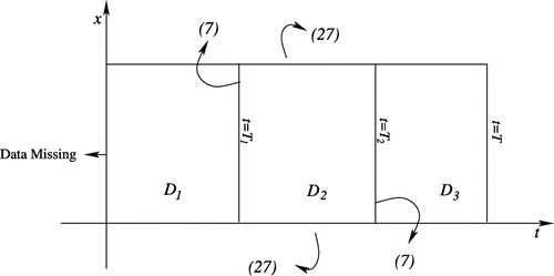First, we assume that the given boundary conditions are28 $$\begin{array}{c}\hfill A(0,t)=A(l,t)=0,0\le t\le T,\end{array}$$28 and the compatibility conditions are given as29 $$\begin{array}{c}\hfill {\mathit{\psi }}_1(0)={\mathit{\psi }}_1(l)={\mathit{\psi }}_2(0)={\mathit{\psi }}_2(l)=0.\end{array}$$29 The key note in applying the procedure, first goes in visualizing the problem domain as is shown Figure 1. Here we assume that the solution has the following format30 $$\begin{array}{c}\hfill \overline{A(x,t)}=\left\{\begin{array}{cc}\overline{A_1(x,t)},\hfill & (x,t)\in D_1,\hfill \\ \overline{A_2(x,t)},\hfill & (x,t)\in D_2,\hfill \\ \overline{A_3(x,t)},\hfill & (x,t)\in D_3,\hfill \end{array}\right.\end{array}$$30

Figure 1. The computational domain for IP2 in the presence of the unknown heat source.

where$$D_1=\{(x,t)|0<x<l,0<t<T_1\},D_2=\{(x,t)|0<x<l,T_1<t<T_2\},$$$$D_3=\{(x,t)|0<x<l,T_2<t<T\}.$$Considering the main equation as31 $$\begin{array}{c}\hfill \frac{\mathit{\partial }A}{\mathit{\partial }t}-\frac{{\mathit{\partial }}^{2}A}{\mathit{\partial }{x}^2}=f(x),\end{array}$$31 and integrating (3030 $$\begin{array}{c}\hfill \overline{A(x,t)}=\left\{\begin{array}{cc}\overline{A_1(x,t)},\hfill & (x,t)\in D_1,\hfill \\ \overline{A_2(x,t)},\hfill & (x,t)\in D_2,\hfill \\ \overline{A_3(x,t)},\hfill & (x,t)\in D_3,\hfill \end{array}\right.\end{array}$$30 ) over the interval $[T_1,T_2]$ and using the extra observations (77 $$\begin{array}{c}\hfill A(x,T_1)={\mathit{\psi }}_1(x),A(x,T_2)={\mathit{\psi }}_2(x).\end{array}$$7 ) we get32 $$\begin{array}{cc}& {\int }_{[T_1,T_2]}\left\{\frac{\mathit{\partial }A(x,s)}{\mathit{\partial }s},-,\frac{{\mathit{\partial }}^{2}A(x,s)}{\mathit{\partial }{x}^2},-,f,(x)\right\}ds={\mathit{\psi }}_2(x)-{\mathit{\psi }}_1(x)\hfill \\ & -{\int }_{[T_1,T_2]}\frac{{\mathit{\partial }}^{2}A(x,s)}{\mathit{\partial }{x}^2}ds-(T_2-T_1)f(x)=0.\hfill \end{array}$$32 Thus we have33 $$\begin{array}{c}\hfill f(x)=\frac{1}{T_2-T_1}\left\{{\mathit{\psi }}_2,(x),-,{\mathit{\psi }}_1,(x),-,{\int }_{[T_1,T_2]},\frac{{\mathit{\partial }}^{2}A(x,s)}{\mathit{\partial }{x}^2},d,s\right\}.\end{array}$$33 Hereafter, our scheme will be proceeded by constructing the Ritz-type approximations$$\overline{A_1(x,t)},\overline{A_2(x,t)},\overline{A_3(x,t)},$$for the following subproblems, respectively.34 $$\begin{array}{c}\hfill SP1:\left\{\begin{array}{cc}{\displaystyle \frac{\mathit{\partial }{A}_1}{\mathit{\partial }t}-\frac{{\mathit{\partial }}^2{A}_1}{\mathit{\partial }{x}^2}=f(x),}\hfill & (x,t)\in D_1,\hfill \\ A_1(0,t)=A_1(l,t)=0,A_1(x,T_1)={\mathit{\psi }}_1(x),\hfill & 0\le x\le l,0\le t\le T_1,\hfill \end{array}\right.\end{array}$$34 35 $$\begin{array}{c}\hfill SP2:\left\{\begin{array}{cc}{\displaystyle \frac{\mathit{\partial }{A}_2}{\mathit{\partial }t}-\frac{{\mathit{\partial }}^2{A}_2}{\mathit{\partial }{x}^2}=\frac{1}{T_2-T_1}\left\{{\displaystyle {\mathit{\psi }}_2(x)-{\mathit{\psi }}_1(x)-{\int }_{[T_1,T_2]}\frac{{\mathit{\partial }}^2{A}_2(x,s)}{\mathit{\partial }{x}^2}ds}\right\},}\hfill & (x,t)\in D_2,\\ A_2(0,t)=A_2(l,t)=0,A_2(x,T_1)={\mathit{\psi }}_1(x),A_2(x,T_2)={\mathit{\psi }}_2(x)\&0\le x\le l,T_1\le t\le T_2,\hfill \end{array}\right.\end{array}$$35 36 $$\begin{array}{c}\hfill SP3:\left\{\begin{array}{c}{\displaystyle \frac{\mathit{\partial }{A}_3}{\mathit{\partial }t}-\frac{{\mathit{\partial }}^2{A}_3}{\mathit{\partial }{x}^2}=f(x),(x,t)\in D_3,}\hfill \\ A_3(0,t)=A_3(l,t)=0,A_3(x,T_2)={\mathit{\psi }}_2(x),0\le x\le l,T_2\le t\le T.\hfill \end{array}\right.\end{array}$$36 Among these three subproblems, SP1, SP3 are backward and forward in time, respectively, while SP2 can be considered as an integro-differential equation.[50] On top of that, it is obviously over-specified because of the extra boundary conditions in (3434 $$\begin{array}{c}\hfill SP1:\left\{\begin{array}{cc}{\displaystyle \frac{\mathit{\partial }{A}_1}{\mathit{\partial }t}-\frac{{\mathit{\partial }}^2{A}_1}{\mathit{\partial }{x}^2}=f(x),}\hfill & (x,t)\in D_1,\hfill \\ A_1(0,t)=A_1(l,t)=0,A_1(x,T_1)={\mathit{\psi }}_1(x),\hfill & 0\le x\le l,0\le t\le T_1,\hfill \end{array}\right.\end{array}$$34 ). Thus, we start with this problem and try to find the approximate solution for $A_2(x,t)$. A Ritz-type approximation can be introduced by37 $$\begin{array}{c}\hfill \overline{A_2(x,t)}=\sum _{i_1=-m+1}^{2^M-1}\sum _{i_2=-n+1}^{2^N-1}x(x-l)(t-T_1)(t-T_2)d_{i_1{i}_2}{\mathit{\varphi }}_{m,i_1}^{(M)}(x){\mathit{\varphi }}_{n,i_2}^{(N)}(t)+s_2(x,t),\end{array}$$37 $$s_2(x,t)={\mathit{\psi }}_1(x)+\frac{t-T_1}{T_2-T_1}\{{\mathit{\psi }}_2(x)-{\mathit{\psi }}_1(x)\}.$$Now similar to (2323 $$\begin{array}{cc}\hfill Res(\overline{B(x,t)})& :=\frac{\mathit{\partial }\overline{B(x,t)}}{\mathit{\partial }t}-\frac{\mathit{\partial }}{\mathit{\partial }x}\left\{k,(x),\frac{\mathit{\partial }\overline{B(x,t)}}{\mathit{\partial }x}\right\}-\frac{1}{\mathit{\delta }(x^{\ast })}\hfill \end{array}$$23 ), we form the residual function38 $$\begin{array}{c}\hfill Res(\overline{A_2(x,t)}):=\frac{\mathit{\partial }\overline{A_2(x,t)}}{\mathit{\partial }t}-\frac{{\mathit{\partial }}^2\overline{A_2(x,t)}}{\mathit{\partial }{x}^2}-\frac{1}{T_2-T_1}\{{\mathit{\psi }}_2(x)-{\mathit{\psi }}_1(x)-{\int }_{[T_1,T_2]}\frac{{\mathit{\partial }}^2\overline{A_2(x,s)}}{\mathit{\partial }{x}^2}ds\},\end{array}$$38 by applying the Galerkin equations39 $$\begin{array}{c}\hfill GEs:=〈R,e,s,(\overline{A_2(x,t)}),,,{\mathit{\varphi }}_{m,i_1}^{(M)},(x),{\mathit{\varphi }}_{n,i_2}^{(N)},(t)〉=0,\end{array}$$39 $$i_1=\overline{-m+1,2^M-1},i_2=\overline{-n+1,2^N-1},$$where$$〈f,g〉=\int f(x)g(x)dx.$$Solving the obtained final systems of equations for elements$$d_{i_1{i}_2},i_1=\overline{-m+1,2^M-1},i_2=\overline{-n+1,2^N-1},$$$\overline{A_2(x,t)}$ is determined. Substituting $\overline{A_2(x,t)}$ in (3232 $$\begin{array}{cc}& {\int }_{[T_1,T_2]}\left\{\frac{\mathit{\partial }A(x,s)}{\mathit{\partial }s},-,\frac{{\mathit{\partial }}^{2}A(x,s)}{\mathit{\partial }{x}^2},-,f,(x)\right\}ds={\mathit{\psi }}_2(x)-{\mathit{\psi }}_1(x)\hfill \\ & -{\int }_{[T_1,T_2]}\frac{{\mathit{\partial }}^{2}A(x,s)}{\mathit{\partial }{x}^2}ds-(T_2-T_1)f(x)=0.\hfill \end{array}$$32 ), we attain40 $$\begin{array}{c}\hfill \overline{f(x)}=\frac{1}{T_2-T_1}\left\{{\mathit{\psi }}_2,(x),-,{\mathit{\psi }}_1,(x),-,{\int }_{[T_1,T_2]},\frac{{\mathit{\partial }}^2\overline{A_2(x,s)}}{\mathit{\partial }{x}^2},d,s\right\}.\end{array}$$40 Henceforth, we use $\overline{f(x)}$ to produce the satisfactory approximations for $A_1(x,t),A_3(x,t)$. It is worth noting that a good approximation for $\overline{A_2(x,t)},\overline{f(x)}$ may lead to get more acceptable approximations for $\overline{A_1(x,t)},\overline{A_3(x,t)}$ and finally $\overline{A_1(x,0)}$. Now we present the following approximations for $A_3(x,t),A_1(x,t)$41 $$\begin{array}{c}\hfill \overline{A_3(x,t)}=\sum _{i_1=-m+1}^{2^M-1}\sum _{i_2=-n+1}^{2^N-1}x(x-l)(t-T_2)d_{i_1{i}_2}{\mathit{\varphi }}_{m,i_1}^{(M)}(x){\mathit{\varphi }}_{n,i_2}^{(N)}(t)+{\mathit{\psi }}_2(x),\end{array}$$41 42 $$\begin{array}{c}\hfill \overline{A_1(x,t)}=\sum _{i_1=-m+1}^{2^M-1}\sum _{i_2=-n+1}^{2^N-1}x(x-l)(t-T_1)d_{i_1{i}_2}{\mathit{\varphi }}_{m,i_1}^{(M)}(x){\mathit{\varphi }}_{n,i_2}^{(N)}(t)+{\mathit{\psi }}_1(x),\end{array}$$42 then constructing the residual functions43 $$\begin{array}{c}\hfill Res(\overline{A_1(x,t)}):=\frac{\mathit{\partial }\overline{A_1(x,t)}}{\mathit{\partial }t}-\frac{{\mathit{\partial }}^2\overline{A_1(x,t)}}{\mathit{\partial }{x}^2}-\overline{f(x)},\end{array}$$43 44 $$\begin{array}{c}\hfill Res(\overline{A_3(x,t)}):=\frac{\mathit{\partial }\overline{A_3(x,t)}}{\mathit{\partial }t}-\frac{{\mathit{\partial }}^2\overline{A_3(x,t)}}{\mathit{\partial }{x}^2}-\overline{f(x)},\end{array}$$44 and contributing Equations (4242 $$\begin{array}{c}\hfill \overline{A_1(x,t)}=\sum _{i_1=-m+1}^{2^M-1}\sum _{i_2=-n+1}^{2^N-1}x(x-l)(t-T_1)d_{i_1{i}_2}{\mathit{\varphi }}_{m,i_1}^{(M)}(x){\mathit{\varphi }}_{n,i_2}^{(N)}(t)+{\mathit{\psi }}_1(x),\end{array}$$42 ) and (4343 $$\begin{array}{c}\hfill Res(\overline{A_1(x,t)}):=\frac{\mathit{\partial }\overline{A_1(x,t)}}{\mathit{\partial }t}-\frac{{\mathit{\partial }}^2\overline{A_1(x,t)}}{\mathit{\partial }{x}^2}-\overline{f(x)},\end{array}$$43 ) in the Galerkin equations similar to (3838 $$\begin{array}{c}\hfill Res(\overline{A_2(x,t)}):=\frac{\mathit{\partial }\overline{A_2(x,t)}}{\mathit{\partial }t}-\frac{{\mathit{\partial }}^2\overline{A_2(x,t)}}{\mathit{\partial }{x}^2}-\frac{1}{T_2-T_1}\{{\mathit{\psi }}_2(x)-{\mathit{\psi }}_1(x)-{\int }_{[T_1,T_2]}\frac{{\mathit{\partial }}^2\overline{A_2(x,s)}}{\mathit{\partial }{x}^2}ds\},\end{array}$$38 ) and solving the final systems of equations, we find the Ritz–Galerkin approximations for ${\{A_w(x,t)\}}_{w=\overline{1,3}}$. Considering Equation (2929 $$\begin{array}{c}\hfill {\mathit{\psi }}_1(0)={\mathit{\psi }}_1(l)={\mathit{\psi }}_2(0)={\mathit{\psi }}_2(l)=0.\end{array}$$29 ), these approximations now can be integrated as a global solution for the whole domain $\overline{A(x,t)}$ and the initial condition i.e. $A(x,0)\simeq \overline{A_1(x,0)}$ can be calculated.

4.3 The solution of IP3

Consider the inverse problem given by Equations (88 $$\begin{array}{c}\hfill \mathit{\rho }(x,t)A_t-\mathrm{\Delta }A=S(x,t),\mathrm{in}\mathrm{\Omega }\times [0,T],\end{array}$$8 ) and (99 $$\begin{array}{c}\hfill A(x,0)=A_0(x),x\in \mathrm{\Omega },\end{array}$$9 ) and (1111 $$\begin{array}{c}\hfill A(x,T)=r(x),x\in \mathrm{\Omega },\end{array}$$11 ) and (1212 $$\begin{array}{c}\hfill A(0,t)=\mathit{\phi }(t),A(1,t)=\mathit{\psi }(t),0\le t\le T,\end{array}$$12 ). We assume that the following compatibility conditions hold45 $$\begin{array}{c}\hfill A_0(0)=\mathit{\phi }(0),A_0(1)=\mathit{\psi }(0),\mathit{\phi }(T)=r(0),\mathit{\psi }(T)=r(1).\end{array}$$45 In comparison to IP1, IP2, here finding the satisfier function which fulfils all the initial and boundary conditions seems to be found more difficult. This is due to the existence of the nonhomogenous Dirichlet boundary conditions. Thus we start the scheme by introducing two functions $s_1^{\ast }(x,t),s_2^{\ast }(x,t)$ as46 $$\begin{array}{c}\hfill s_1^{\ast }(x,t)=\mathit{\phi }(t)+x\{\mathit{\psi }(t)-\mathit{\phi }(t)\},\end{array}$$46 47 $$\begin{array}{c}\hfill s_2^{\ast }(x,t)=A_0(x)+\frac{t}{T}\{r(x)-A_0(x)\}-\left\{s_1^{\ast },(x,0),+,\frac{t}{T},(s_1^{\ast }(x,T)-s_1^{\ast }(x,0))\right\}+s_1^{\ast }(x,t).\end{array}$$47 To achieve the goal of presenting the solution of the problem, we introduce the approximations sought in the form of the truncated series:48 $$\begin{array}{c}\hfill \overline{A(x,t)}=\sum _{n_1=0}^{k_1-1}\sum _{n_2=0}^{k_2-1}\sum _{i_1=0}^{m_1}\sum _{i_2=0}^{m_2}t(t-T)x(x-1)c_{i_1,i_2,n_1,n_2}{\mathit{\psi }}_{i,n}(x,t)+s_2^{\ast }(x,t),\end{array}$$48 49 $$\begin{array}{c}\hfill \overline{f(x)}=\sum _{n_3=0}^{k_3-1}\sum _{i_3=0}^{m_3}{d}_{i_3,n_3}{\mathit{\psi }}_{i_3,n_3}(x).\end{array}$$49 Considering the compatibility conditions (4444 $$\begin{array}{c}\hfill Res(\overline{A_3(x,t)}):=\frac{\mathit{\partial }\overline{A_3(x,t)}}{\mathit{\partial }t}-\frac{{\mathit{\partial }}^2\overline{A_3(x,t)}}{\mathit{\partial }{x}^2}-\overline{f(x)},\end{array}$$44 ), (4747 $$\begin{array}{c}\hfill s_2^{\ast }(x,t)=A_0(x)+\frac{t}{T}\{r(x)-A_0(x)\}-\left\{s_1^{\ast },(x,0),+,\frac{t}{T},(s_1^{\ast }(x,T)-s_1^{\ast }(x,0))\right\}+s_1^{\ast }(x,t).\end{array}$$47 ) satisfies all the initial and boundary conditions (99 $$\begin{array}{c}\hfill A(x,0)=A_0(x),x\in \mathrm{\Omega },\end{array}$$9 ) and (1111 $$\begin{array}{c}\hfill A(x,T)=r(x),x\in \mathrm{\Omega },\end{array}$$11 ) and (1212 $$\begin{array}{c}\hfill A(0,t)=\mathit{\phi }(t),A(1,t)=\mathit{\psi }(t),0\le t\le T,\end{array}$$12 ), where ${\mathit{\psi }}_{i,n}(X)=B_{i_1,m_1}(k_{1}x-n_1)B_{i_2,m_2}(\frac{k_{2}t}{T}-n_2)$. Substituting (4747 $$\begin{array}{c}\hfill s_2^{\ast }(x,t)=A_0(x)+\frac{t}{T}\{r(x)-A_0(x)\}-\left\{s_1^{\ast },(x,0),+,\frac{t}{T},(s_1^{\ast }(x,T)-s_1^{\ast }(x,0))\right\}+s_1^{\ast }(x,t).\end{array}$$47 ) and (4848 $$\begin{array}{c}\hfill \overline{A(x,t)}=\sum _{n_1=0}^{k_1-1}\sum _{n_2=0}^{k_2-1}\sum _{i_1=0}^{m_1}\sum _{i_2=0}^{m_2}t(t-T)x(x-1)c_{i_1,i_2,n_1,n_2}{\mathit{\psi }}_{i,n}(x,t)+s_2^{\ast }(x,t),\end{array}$$48 ) in (88 $$\begin{array}{c}\hfill \mathit{\rho }(x,t)A_t-\mathrm{\Delta }A=S(x,t),\mathrm{in}\mathrm{\Omega }\times [0,T],\end{array}$$8 ), we find50 $$\begin{array}{c}\hfill Res(\overline{A(x,t)};\overline{f(x)}):=\mathit{\rho }(x,t)\overline{A_t}-\mathrm{\Delta }\overline{A}-\overline{f(x)}g(x,t)-h(x,t),\end{array}$$50 and applying the simultaneous Galerkin equations51 $$\begin{array}{c}\hfill GEs:\left\{\begin{array}{c}〈R,e,s,(\overline{A(x,t)};\overline{f(x)}),,,B_{i_1,m_1},(k_{1}x-n_1),B_{i_2,m_2},\left(\frac{k_{2}t}{T},-,n_2\right)〉=0,\hfill \\ i_s=0,1,...,m_s,s\in \{1,2\},\hfill \\ {\int }_{D_{i_3{n}_3}}Res(\overline{A(x,t)};\overline{f(x)})Heaviside(D_{i_3{n}_3})dx=0,i_3=0,1,...,m_3,\hfill & \hfill \end{array}\right.\end{array}$$51 where $D_{i_3{n}_3}$ is the partitioned part of the space and52 $$\begin{array}{c}\hfill Heaviside(D_{i_3{n}_3})=\left\{\begin{array}{cc}1\hfill & x\in D_{i_3{n}_3},\hfill \\ 0\hfill & \mathrm{otherwise},\hfill \end{array}\right.\end{array}$$52 we obtain a system of linear equations for the elements $c_{i_1,i_2,n_1,n_2},d_{i_3,n_3},i_1=0,1,...,m_1,i_2=0,1,...,m_2,i_3=0,1,...,m_3,n_1=0,1,...,k_1-1,n_2=0,1,...,k_2-1,n_3=0,1,...,k_3-1.$ What stated as the satisfier function, here presented as $s_2^{\ast }(x,t)$, is not unique in general. Overall, constructing this function can be found using the interpolation techniques. Besides, the physical information of the problem can be useful to obtain the appropriate function that is close enough to the exact solution. Nevertheless, assuming that the solution has the product form,[49] under some restrictions we find the unique function.

Lemma 4.1

If each of the following conditions$$\mathit{\varphi }(0)\ne 0,\mathit{\psi }(0)\ne 0,r(0)\ne 0,r(1)\ne 0,$$holds, then the separable satisfier function for the product solution of IP3 is unique.

Proof

Suppose that the satisfier function found for the Ritz–Galerkin solution of problem IP3 is known as $u(x)v(t)$. If there exists another function as $u_1(x)v_1(t)$, then considering (99 $$\begin{array}{c}\hfill A(x,0)=A_0(x),x\in \mathrm{\Omega },\end{array}$$9 ) we have53 $$\begin{array}{c}\hfill u_1(x)v_1(0)=u(x)v(0),\end{array}$$53 on the other hand from (1212 $$\begin{array}{c}\hfill A(0,t)=\mathit{\phi }(t),A(1,t)=\mathit{\psi }(t),0\le t\le T,\end{array}$$12 ) we get54 $$\begin{array}{c}\hfill u_1(1)v_1(t)=u(1)v(t).\end{array}$$54 Multiplying (5252 $$\begin{array}{c}\hfill Heaviside(D_{i_3{n}_3})=\left\{\begin{array}{cc}1\hfill & x\in D_{i_3{n}_3},\hfill \\ 0\hfill & \mathrm{otherwise},\hfill \end{array}\right.\end{array}$$52 ) with (5353 $$\begin{array}{c}\hfill u_1(x)v_1(0)=u(x)v(0),\end{array}$$53 ), we obtain55 $$\begin{array}{c}\hfill u(x)v(0)u(1)v(t)=u_1(x)v_1(0)u_1(1)v_1(t).\end{array}$$55 Now considering $0\ne \mathit{\psi }(0)=u(1)v(0)=u_1(1)v_1(0)$, from (5454 $$\begin{array}{c}\hfill u_1(1)v_1(t)=u(1)v(t).\end{array}$$54 ) we conclude$$u(x)v(t)-u_1(x)v_1(t)=0.$$Similar to this statement we can say that the assertion of the lemma can be confirmed when $\mathit{\varphi }(0)\ne 0,r(0)\ne 0,r(1)\ne 0$. $\square$

Remark 4.1

In inverse problems a remarkable attention is devoted to the stability of the solution for the presented algorithms. Indeed, although the unique solution may hold under certain restrictions on the input data, the inverse problem is still ill-posed since small errors in the measured data cause rather large errors in the output solution. Thus the authors try to find a priori bound, namely, the stability estimate for solution, to be assured of this fact that the solution depends on some upper bound containing the initial or either boundary data. For evolutionary equations, the Gronwall’s lemma is of significance.[1] Here, we restrict ourselves to this lemma formulated in its simplest form.

Lemma

For a function $g(t)$ satisfying the inequality56 $$\begin{array}{c}\hfill \frac{dg}{dt}\le ag(t)+b(t),t>0,\end{array}$$56 with $a=const$ and $b(t)\ge 0$, the following estimate holds:57 $$\begin{array}{c}\hfill g(t)\le e^{at}\{g(0)+{\int }_{[0,t]}{e}^{-a\mathit{\tau }}b(\mathit{\tau })d\mathit{\tau }\}.\end{array}$$57

Corollary

Consider the Cauchy problem for a first-order operator differential equation58 $$\begin{array}{c}\hfill \frac{dA}{dt}+\mathcal{F}A=f,\end{array}$$58 $$A(0)=A_0,$$with the self-adjoint, positive operator $\mathcal{F}$. Then the following estimation of the stable solution with respect to initial data and the right-hand side is obtained:59 $$\begin{array}{c}\hfill {\Vert A(t)\Vert }^2\le exp(t)\{\Vert A_0{\Vert }^2+{\int }_{[0,t]}{exp(-s)\Vert f(s)\Vert }^{2}ds\}.\end{array}$$59

Proof

From scalarwise multiplying equation (5757 $$\begin{array}{c}\hfill g(t)\le e^{at}\{g(0)+{\int }_{[0,t]}{e}^{-a\mathit{\tau }}b(\mathit{\tau })d\mathit{\tau }\}.\end{array}$$57 ) by $A(t)$ we get [1]60 $$\begin{array}{c}\hfill 〈\frac{dA}{dt},,,A〉+〈\mathcal{F}A,A〉=〈f,A〉.\end{array}$$60 On the other hand, applying the Cauchy–Bunyakowsky inequality, we have:61 $$\begin{array}{c}\hfill 〈f,A〉\le \Vert f\Vert \Vert A\Vert ,〈\frac{dA}{dt},,,A〉=\int \frac{dA}{dt}Adt=\frac{1}{2}\frac{d}{dt}\int A^{2}dt=\frac{1}{2}\frac{d}{dt}{\Vert A\Vert }^2.\end{array}$$61 Taking (6060 $$\begin{array}{c}\hfill 〈\frac{dA}{dt},,,A〉+〈\mathcal{F}A,A〉=〈f,A〉.\end{array}$$60 ) into account, (5959 $$\begin{array}{c}\hfill {\Vert A(t)\Vert }^2\le exp(t)\{\Vert A_0{\Vert }^2+{\int }_{[0,t]}{exp(-s)\Vert f(s)\Vert }^{2}ds\}.\end{array}$$59 ) becomes62 $$\begin{array}{c}\hfill \frac{1}{2}\frac{d}{dt}{\Vert A\Vert }^2\le \Vert f\Vert \Vert A\Vert \le \frac{1}{2}{\{\Vert A\Vert }^2+{\Vert f\Vert }^2\}.\end{array}$$62 Comparing (6161 $$\begin{array}{c}\hfill 〈f,A〉\le \Vert f\Vert \Vert A\Vert ,〈\frac{dA}{dt},,,A〉=\int \frac{dA}{dt}Adt=\frac{1}{2}\frac{d}{dt}\int A^{2}dt=\frac{1}{2}\frac{d}{dt}{\Vert A\Vert }^2.\end{array}$$61 ) with Lemma 4.2 by setting $a=1$ and $g(t)={\Vert A(t)\Vert }^2$, we find the estimation (5858 $$\begin{array}{c}\hfill \frac{dA}{dt}+\mathcal{F}A=f,\end{array}$$58 ). $\square$

Remark 4.2

Mathematically speaking, the inverse problems typically lead to models that are ill-posed or improperly posed in the sense of Hadamard. This means especially that noise in measurement data may lead to significant misinterpretations of the solution.[51] Therefore, appropriate procedure should be employed to find trusted solutions. Here, we utilize the Tikhonov regularization method to overcome the stability and solving the final systems of equations $A\underline{x}=b$, in the general form, produced by Galerkin Equations (2424 $$\begin{array}{cc}& \left\{\mathit{\phi },(t),-,\overline{B(x^{\ast },t)}\right\}\frac{\mathit{\partial }}{\mathit{\partial }x}\left\{k,(x),\frac{\mathit{\partial }\mathit{\delta }}{\mathit{\partial }x}\right\},\hfill \end{array}$$24 ), (3838 $$\begin{array}{c}\hfill Res(\overline{A_2(x,t)}):=\frac{\mathit{\partial }\overline{A_2(x,t)}}{\mathit{\partial }t}-\frac{{\mathit{\partial }}^2\overline{A_2(x,t)}}{\mathit{\partial }{x}^2}-\frac{1}{T_2-T_1}\{{\mathit{\psi }}_2(x)-{\mathit{\psi }}_1(x)-{\int }_{[T_1,T_2]}\frac{{\mathit{\partial }}^2\overline{A_2(x,s)}}{\mathit{\partial }{x}^2}ds\},\end{array}$$38 ), (4242 $$\begin{array}{c}\hfill \overline{A_1(x,t)}=\sum _{i_1=-m+1}^{2^M-1}\sum _{i_2=-n+1}^{2^N-1}x(x-l)(t-T_1)d_{i_1{i}_2}{\mathit{\varphi }}_{m,i_1}^{(M)}(x){\mathit{\varphi }}_{n,i_2}^{(N)}(t)+{\mathit{\psi }}_1(x),\end{array}$$42 ), (4343 $$\begin{array}{c}\hfill Res(\overline{A_1(x,t)}):=\frac{\mathit{\partial }\overline{A_1(x,t)}}{\mathit{\partial }t}-\frac{{\mathit{\partial }}^2\overline{A_1(x,t)}}{\mathit{\partial }{x}^2}-\overline{f(x)},\end{array}$$43 ), and (5050 $$\begin{array}{c}\hfill Res(\overline{A(x,t)};\overline{f(x)}):=\mathit{\rho }(x,t)\overline{A_t}-\mathrm{\Delta }\overline{A}-\overline{f(x)}g(x,t)-h(x,t),\end{array}$$50 ). The conventional Tikhonov regularization method is equivalent to solve an unconstrained optimization problem,[52]63 $$\begin{array}{c}\hfill \underline{x}=argminJ(\mathit{\alpha },x)=\frac{1}{2}\Vert A\underline{x}{-b\Vert }_2^2+\frac{\mathit{\alpha }}{2}{\Vert \underline{x}\Vert }_2^2.\end{array}$$63 The main problem in applying (6262 $$\begin{array}{c}\hfill \frac{1}{2}\frac{d}{dt}{\Vert A\Vert }^2\le \Vert f\Vert \Vert A\Vert \le \frac{1}{2}{\{\Vert A\Vert }^2+{\Vert f\Vert }^2\}.\end{array}$$62 ) is finding the regularization parameter $\mathit{\alpha }$, attracted the attention of several authors.[1, 51, 53] Here, we solve (6262 $$\begin{array}{c}\hfill \frac{1}{2}\frac{d}{dt}{\Vert A\Vert }^2\le \Vert f\Vert \Vert A\Vert \le \frac{1}{2}{\{\Vert A\Vert }^2+{\Vert f\Vert }^2\}.\end{array}$$62 ) by employing an iterative procedure known as trust region method and adjusts the trust region radius instead of adjusting the parameter, see chapter 12 in [52]. The method indirectly solves64 $$\begin{array}{c}\hfill \underset{x\in X}{min}{\Vert A\underline{x}-b\Vert }_2^2.\end{array}$$64 It means that the algorithm takes a trial step from a subproblem at each iteration65 $$\begin{array}{c}\hfill J=\underset{z\in X}{min}{\mathrm{\Phi }}_k(z),\end{array}$$65 66 $$\begin{array}{c}\hfill \left\{\begin{array}{c}{min}_{z\in X}{\mathrm{\Phi }}_k(z)=z^{T}gra{d}_k[J]+\frac{1}{2}{z}^{T}Hes{s}_k[J]z,\hfill \\ \mathrm{s}.\mathrm{t}\Vert z\Vert \le {\mathrm{\Delta }}_k,\hfill \end{array}\right.\end{array}$$66 where67 $$\begin{array}{c}\hfill gra{d}_k[J]={(A^{T}A)}^{-1}{\underline{x}}_k-A^{T}b,Hes{s}_k[J]=A^{T}A,\end{array}$$67 are the gradient and Hessian matrices, ${\mathrm{\Delta }}_k>0$ is a trust region radius at the $k$-th iteration. The algorithm typically takes [52]68 $$\begin{array}{c}\hfill {\underline{x}}_0,{\mathrm{\Delta }}_0>0.\end{array}$$68 As the first step, setting $k=0$, taking into account the positive initial values $x_0,{\mathrm{\Delta }}_0$ and solving the minimization problem (6565 $$\begin{array}{c}\hfill J=\underset{z\in X}{min}{\mathrm{\Phi }}_k(z),\end{array}$$65 ) i.e.69 $$\begin{array}{c}\hfill \left\{\begin{array}{c}{min}_{z\in X}{\mathrm{\Phi }}_0(z)=z^{T}gra{d}_0[J]+\frac{1}{2}{z}^{T}Hes{s}_0[J]z,\hfill \\ \mathrm{s}.\mathrm{t}\Vert z\Vert \le {\mathrm{\Delta }}_0,\hfill \end{array}\right.\end{array}$$69 where70 $$\begin{array}{c}\hfill gra{d}_0[J]={(A^{T}A)}^{-1}{\underline{x}}_0-A^{T}b,Hes{s}_0[J]=A^{T}A,\end{array}$$70 we find the desired value $z_0$ for this stage. Now put ${\underline{x}}_1={\underline{x}}_0+z_0$ and calculate$${\mathrm{\Theta }}_1=\Vert A{\underline{x}}_1-b\Vert .$$If ${\mathrm{\Theta }}_1<{\mathit{\epsilon }}_s$, the algorithm can be stopped, otherwise setting $k\ge 1$ and solving (6565 $$\begin{array}{c}\hfill J=\underset{z\in X}{min}{\mathrm{\Phi }}_k(z),\end{array}$$65 ) we get $z_k$. Now for each $k\ge 1$ set ${\underline{x}}_{k+1}={\underline{x}}_k+z_k$, where ${\mathrm{\Delta }}_{k+1}\in [\frac{\Vert z_k\Vert }{4},\frac{{\mathrm{\Delta }}_k}{2}]$. At each step $m\ge 1$ we evaluate$${\mathrm{\Theta }}_m=\Vert A{\underline{x}}_m-b\Vert ,$$to figure out that the obtained vector ${\underline{x}}_m$ satisfies the stopping criterion71 $$\begin{array}{c}\hfill \Vert A{\underline{x}}_m-b\Vert <{\mathit{\epsilon }}_s.\end{array}$$71 If so, the iteration is terminated. Otherwise the procedure is continued until we find the satisfactory result by means of (7070 $$\begin{array}{c}\hfill gra{d}_0[J]={(A^{T}A)}^{-1}{\underline{x}}_0-A^{T}b,Hes{s}_0[J]=A^{T}A,\end{array}$$70 ). For more background on this method and solving the non-linear problems, we refer the interested reader to [52] and its related references.

5 Numerical results and discussion

To show the applicability of the presented schemes for the discussed inverse problems, we solve three benchmark test examples. Examples 5.1–5.3 are chosen for reporting the results of implementing the Ritz–Galerkin technique for IP1–IP3, respectively. For all examples, the exact solutions are available. We investigated the accuracy and stability of the method presented in this paper by performing the mentioned methods for different numbers of the bases in the presence of various amount of noise. It can be seen, that applying the Ritz–Galerkin method along with the satisfier function we find satisfactory results. Meanwhile it should be noted that the final systems of equations are solved using the proposed technique in Remark 4.2 with the convenient stopping criterion fixed on ${\mathit{\epsilon }}_s={10}^{-6}$ for all numerical experiments. Besides, choosing the initial guess for starting the process is arbitrary while we take all starting guesses as the vector ${\underline{x}}_0={\underbrace{(1,...,1)}}_{\in {\mathbb{R}}^p}$, where $p$ is the number of unknown coefficients and solve the optimization problem (6565 $$\begin{array}{c}\hfill J=\underset{z\in X}{min}{\mathrm{\Phi }}_k(z),\end{array}$$65 ) at each step using the FindMinimum command in MATHEMATICA. The numerical implementation is carried out in MATHEMATICA 7, with hardware configuration: desktop 32-bit Intel Core 2 Duo CPU, 4 GB of RAM, 32-bit Operating System (Windows 7).

5.1 Example 1

As the first example, consider IP1 given by Equations (11 $$\begin{array}{c}\hfill \frac{\mathit{\partial }A}{\mathit{\partial }t}-\frac{\mathit{\partial }}{\mathit{\partial }x}\left(k,(x),\frac{\mathit{\partial }A}{\mathit{\partial }x}\right)=f(x,t)\mathrm{in}Q=\mathrm{\Omega }\times (0,T],\end{array}$$1 )–(55 $$\begin{array}{c}\hfill f(x,t)=\mathit{\delta }(x)\mathit{\sigma }(t),\end{array}$$5 ) with the following properties$$A_0(x)=sin(\mathit{\pi }x),\mathit{\phi }(t)=2-exp(-{\mathit{\pi }}^{2}t),f(x,t)=2{\mathit{\pi }}^{2}sin(\mathit{\pi }x).$$The implementation of the numerical method presented in Subsection 4.1 will be illustrated below for approximating both functions$$A(x,t)=(2-exp(-{\mathit{\pi }}^{2}t))sin(\mathit{\pi }x),\mathit{\sigma }(t)=1.$$Testifying the numerical convergence of the solution with respect to the number of basis is of our special interest. Thus we apply the Ritz–Galerkin method by employing the Bernstein basis with $k_1=k_2=1$ and $\sqrt{L}=\sqrt{(m_1+1)\times (m_2+1)},(m_1+1)=(m_2+1)\in \{2,3,3,5,6,7\}$. Final systems of equations are solved utilizing the technique presented in Remark 4.2 and the results are given in Figures 2–8 and tabulated in Table 1. Following these consequences, we observe that the accuracy grows as $\sqrt{L}$ increases, this fact can be understood more clear from the data shown in Table 1 since as $\sqrt{L}$ increases, we find the approximations that possess more truly significant digits. This indicates that the numerical solution converges to the exact solution as the number of basis increases gradually. The next issue is examination of the numerical stability. This factor can be tested by contaminating the initial or boundary data with the artificial random errors.[2, 38] Here we generate the noisy data using [54, 55]72 $$\begin{array}{c}\hfill A^{\mathit{ϵ}}(x^{\ast },t)={\mathit{\phi }}^{\mathit{ϵ}}(t)=\mathit{\phi }(t)\times (1+\mathit{ϵ}\mathit{\epsilon }),\end{array}$$72 where $\mathit{ϵ}$ is the percentage of noise and $\mathit{\epsilon }$ is a random real number between $[-1,1]$. We resolve the problem with the imposed random errors $\mathit{ϵ}\in \{1,3,5\}$%, on the additional boundary data to find the approximate solutions utilizing the Ritz–Galerkin method for the problem with$$k_1=k_2=k_3=1,\sqrt{L}=6.$$The results are depicted by Figure 9. From this figure, we observe that the proposed method is sensitive to random errors. Hence the performance of the method degrades in the presence of errors in the additional specification.[22] In other words, as the percentage of the imposed errors decreases, agreement between the exact and approximate solutions becomes uniformly good.

Table 1. Approximate solutions of $\mathit{\sigma }(t)=1$ using the Ritz–Galerkin method discussed in Example 5.1, attained by applying different number of bases in the presence of the noiseless data corresponded to Example 5.1.

$x$	$\sqrt{L}=2$	$\sqrt{L}=3$	$\sqrt{L}=4$	$\sqrt{L}=5$	$\sqrt{L}=6$	$\sqrt{L}=7$
$0.0000$	$1.1966$	$1.0990$	$1.0432$	$1.0162$	$1.0053$	$1.0015$
$0.1000$	$0.9751$	$0.9674$	$0.9840$	$0.9948$	$0.9991$	$1.0000$
$0.2000$	$0.9347$	$0.9699$	$0.9991$	$1.0032$	$1.0014$	$1.0002$
$0.3000$	$0.9520$	$0.9950$	$1.0099$	$1.0026$	$0.9995$	$0.9996$
$0.4000$	$0.9809$	$1.0082$	$1.0062$	$0.9979$	$0.9989$	$1.0000$
$0.5000$	$1.0043$	$1.0043$	$0.9967$	$0.9967$	$1.0003$	$1.0003$
$0.6000$	$1.0159$	$0.9884$	$0.9916$	$0.9999$	$1.0010$	$0.9998$
$0.7000$	$1.0132$	$0.9701$	$0.9954$	$1.0028$	$0.9998$	$0.9997$
$0.8000$	$0.9953$	$0.9601$	$1.0048$	$1.0006$	$0.9990$	$1.0002$
$0.9000$	$0.9619$	$0.9698$	$1.0071$	$0.9963$	$1.0008$	$0.9999$
$1.0000$	$0.9130$	$1.0109$	$0.9807$	$1.0077$	$0.9971$	$1.0009$

Figure 2. The maximum absolute errors between exact and approximate solutions against the number of basis, i.e. $▽$: $Ma{x}_{0<x<1}(|\mathit{\sigma }(t)-\overline{\mathit{\sigma }(t)}|)$ obtained by the Ritz–Galerkin method with $k_1=k_2=1,\sqrt{L}\in \{2,3,4,5,6,7\}$, related to Example 5.1.

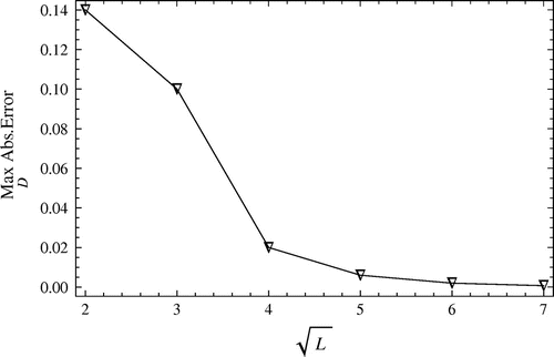
Figure 3. Contour lines corresponding to the absolute error between $[A(x,t),\overline{A(x,t)}]$ when $k_1=k_2=1,\sqrt{L}=2$ for Example 5.1.

Figure 4. Contour lines corresponding to the absolute error between $[A(x,t),\overline{A(x,t)}]$ when $k_1=k_2=1,\sqrt{L}=3$ for Example 5.1.

Figure 5. Contour lines corresponding to the absolute error between $[A(x,t),\overline{A(x,t)}]$ when $k_1=k_2=1,\sqrt{L}=4$ for Example 5.1.

Figure 6. Contour lines corresponding to the absolute error between $[A(x,t),\overline{A(x,t)}]$ when $k_1=k_2=1,\sqrt{L}=5$ for Example 5.1.

Figure 7. Contour lines corresponding to the absolute error between $[A(x,t),\overline{A(x,t)}]$ when $k_1=k_2=1,\sqrt{L}=6$ for Example 5.1.

Figure 8. Contour lines corresponding to the absolute error between $[A(x,t),\overline{A(x,t)}]$ when $k_1=k_2=1,\sqrt{L}=7$ for Example 5.1.

Figure 9. The approximate solutions for $\mathit{\sigma }(t)$ attained by the Ritz-Galerkin method with $k_1=k_2=k_3=1,m_1=m_2=3,m_3=2$ in the presence of different amount errors; $\circ \circ \circ$: The exact solution,   $\bullet \bullet \bullet$: Solution when $\mathit{ϵ}=1\%$,   $\ast \ast \ast$: Solution when $\mathit{ϵ}=3\%$,   $▾▾▾$: Solution when $\mathit{ϵ}=5\%$, related to Example 5.1.

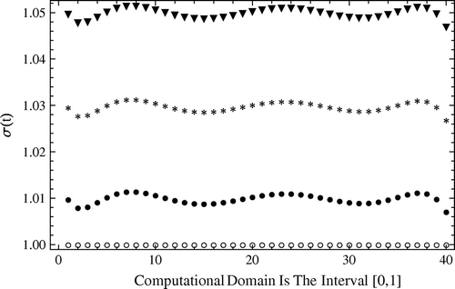
Figure 10. The maximum absolute errors between exact and approximate solutions against the number of basis for $f(x)$, i.e. $\ast$: $Ma{x}_{0<x<1}(|f(x)-\overline{f(x)}|)$ obtained by the Ritz–Galerkin method with $m,n\in \{2,3,4\},M=N=3$, related to Example 5.2.

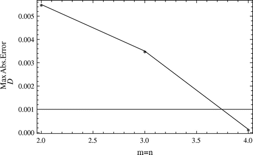
Figure 11. The Maximum absolute errors between exact and approximate solutions against the number of basis for $A(x,0)$, i.e. $▽$: $Ma{x}_{0<x<1}(|A(x,0)-\overline{A(x,0)}|)$ obtained by the Ritz–Galerkin method with $m,n\in \{2,3,4\},M=N=3$, related to Example 5.2.

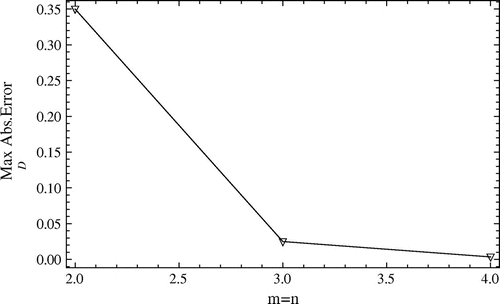
Figure 12. Contour lines corresponding to the absolute error between $[A(x,t),\overline{A(x,t)}]$ when $m=n=2,M=N=3$ for Example 5.2.

Figure 13. Contour lines corresponding to the absolute error between $[A(x,t),\overline{A(x,t)}]$ when $m=n=3,M=N=3$ for Example 5.2.

Figure 14. Contour lines corresponding to the absolute error between $[A(x,t),\overline{A(x,t)}]$ when $m=n=4,M=N=3$ for Example 5.2.

5.2 Example 2

As the second example,[26] we consider IP2 given by Equations (66 $$\begin{array}{c}\hfill \left\{\begin{array}{cc}{\mathit{\partial }}_{t}A+LA=f(x),\hfill & \mathrm{in}\mathrm{\Omega }\times (0,T),\hfill \\ A=0,\hfill & \mathrm{on}\mathrm{\Gamma }\times (0,T),\hfill \\ A(x,0)=\mathit{\phi }(x),\hfill & x\in \mathrm{\Omega },\hfill \end{array}\right.\end{array}$$6 ) and (77 $$\begin{array}{c}\hfill A(x,T_1)={\mathit{\psi }}_1(x),A(x,T_2)={\mathit{\psi }}_2(x).\end{array}$$7 ) with$$\begin{array}{cc}\hfill l=1,\mathit{\phi }(x)& =sin(\mathit{\pi }x),{\mathit{\psi }}_1(x)=\left(2,-,exp,\left(-,\frac{{\mathit{\pi }}^2}{2}\right)\right)sin(\mathit{\pi }x),\hfill \\ \hfill {\mathit{\psi }}_2(x)& =\left(2,-,exp,\left(-,{\mathit{\pi }}^2\right)\right)sin(\mathit{\pi }x).\hfill \end{array}$$The exact solutions for this problem are$$(A(x,t),f(x))=((2-exp(-{\mathit{\pi }}^{2}t))sin(\mathit{\pi }x),2{\mathit{\pi }}^{2}sin(\mathit{\pi }x)),$$which should be recovered. We note that since the additional information is given in $T_1=\frac{1}{2},T_2=T_3=T=1$, the domain of the problem is divided into two subdomains and hereafter we seek the approximations

Table 2. The maximum absolute errors between exact and approximate solutions against the number of basis for $f(x)$ and $A(x,0)$, i.e. $Ma{x}_{0<x<1}(|f(x)-\overline{f(x)}|)$ , $Ma{x}_{0<x<1}(|A(x,0)-\overline{A(x,0)}|)$ obtained by the Ritz–Galerkin method with $m,n\in \{2,3,4\},M=N=3$, related to Example 5.2.

Maximum Absolute Error	$m=n=2$	$m=n=3$	$m=n=4$
$Ma{x}_{0<x<1}(|f(x)-\overline{f(x)}|)$	$0.0055$	$0.0035$	$0.00014$
$Ma{x}_{0<x<1}(|A(x,0)-\overline{A(x,0)}|)$	$0.35$	$0.025$	$0.0031$

$$\overline{A_1(x,t)},(x,t)\in [0,1]\times [0,\frac{1}{2}],\overline{A_2(x,t)},(x,t)\in [0,1]\times \left[\frac{1}{2},,,1\right].$$Applying the Ritz–Galerkin method presented in Subsection 4.2 with$$m,n\in \{2,3,4\},M=N=3,$$we obtain the results shown in Figures 10–14 and tabulated in Table 2. It is seen from the depicted results that the approximations of both $\overline{f(x)},\overline{A(x,0)}$ are improved by increasing$m,n$. Thus, the numerical convergence of the solution is obtained. In other words, raising the order of B-spline basis leads to obtain more accurate approximations. To discuss on the numerical stability of the solution, we again turn back to perturbing the boundary data (77 $$\begin{array}{c}\hfill A(x,T_1)={\mathit{\psi }}_1(x),A(x,T_2)={\mathit{\psi }}_2(x).\end{array}$$7 ) by means of the following law73 $$\begin{array}{c}\hfill {\mathit{\psi }}_1^{{\mathit{\chi }}_1}(x)={\mathit{\psi }}_1(x)\times (1+{\mathit{\chi }}_1\mathit{\epsilon }),{\mathit{\psi }}_2^{{\mathit{\chi }}_2}(x)={\mathit{\psi }}_2(x)\times (1+{\mathit{\chi }}_2\mathit{\epsilon }),\end{array}$$73 and then repeat the solution schedule for the problem with the imposed random errors ${\mathit{\chi }}_1={\mathit{\chi }}_2\in \{1,3,5\}\%$. Now utilizing the Ritz-Galerkin method with$$m=n=3,M=N=3,$$we produce theresults shown in Figures 15–20 and Table 3 as illustration. Comparing the approximations, one can conclude that the stability with respect to boundary data is overcome for different percentages of contaminated errors ${\mathit{\chi }}_1={\mathit{\chi }}_2\in \{1,3,5\}\%$. On the other hand, let turn back to the solution procedure given in Subsection 4.2. Paying attention, we find that contaminating the extra specification ${\mathit{\psi }}_1(x),{\mathit{\psi }}_2(x)$ by artificial errors, first affects the approximation resulted from Equation (3232 $$\begin{array}{cc}& {\int }_{[T_1,T_2]}\left\{\frac{\mathit{\partial }A(x,s)}{\mathit{\partial }s},-,\frac{{\mathit{\partial }}^{2}A(x,s)}{\mathit{\partial }{x}^2},-,f,(x)\right\}ds={\mathit{\psi }}_2(x)-{\mathit{\psi }}_1(x)\hfill \\ & -{\int }_{[T_1,T_2]}\frac{{\mathit{\partial }}^{2}A(x,s)}{\mathit{\partial }{x}^2}ds-(T_2-T_1)f(x)=0.\hfill \end{array}$$32 ). It means that the approximation $\overline{f(x)}$ obtained from Equation (3939 $$\begin{array}{c}\hfill GEs:=〈R,e,s,(\overline{A_2(x,t)}),,,{\mathit{\varphi }}_{m,i_1}^{(M)},(x),{\mathit{\varphi }}_{n,i_2}^{(N)},(t)〉=0,\end{array}$$39 ), contains the errors which at the next step are used to find the approximations for $\overline{A_1(x,t)},\overline{A_2(x,t)}$ due to the direct contribution of $\overline{f(x)}$ in solving SP1, SP2. Thus care enough must be taken in applying the percentage of the imposed errors into the boundary data to produce the trusted and stable solutions. Since involving the high percentage of errors produces a high rate of error propagation in solving the problem. Putting this matter in consideration and noting to results reported by Figures 15–20 and Table 3, we can claim that the new proposed scheme gives the numerical results where the stability with respect to the right-hand side, also is overcome in the presence of the errors ${\mathit{\chi }}_1={\mathit{\chi }}_2\in \{1,3,5\}\%$. Worthy of being considered at the end, here the errors in predicting the initial temperature $A(x,0)$ are larger.[26, 56] Apart from the high ill-posedness of the BHCP in the region $0<t<T_1=\frac{1}{2}$, the solution schedule presented can be effective in the produced errors in finding $\overline{A(x,0)}$. For obtaining more accurate results, it seems that setting $T_1$ closer to $t=0$ and utilizing this observation, we find the numerical solutions which approximate better the exact solution.[26, 57]

Figure 15. The absolute errors between exact and approximate solutions for $f(x)$ against the per cent of noise ${\mathit{\chi }}_1={\mathit{\chi }}_2=1\%$, obtained by the Ritz–Galerkin method with $m=n=3,M=N=3$, related to Example 5.2.

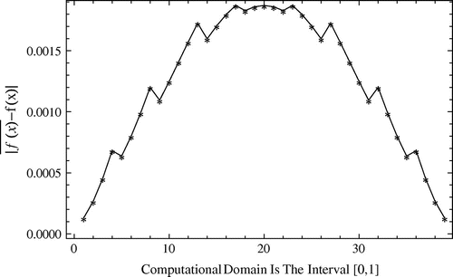
Figure 16. The absolute errors between exact and approximate solutions for $A(x,0)$ against the per cent of noise ${\mathit{\chi }}_1={\mathit{\chi }}_2=1\%$, obtained by the Ritz–Galerkin method with $m=n=3,M=N=3$, related to Example 5.2.

Figure 17. The absolute errors between exact and approximate solutions for $f(x)$ against the per cent of noise ${\mathit{\chi }}_1={\mathit{\chi }}_2=3\%$, obtained by the Ritz–Galerkin method with $m=n=3,M=N=3$, related to Example 5.2.

Figure 18. The absolute errors between exact and approximate solutions for $A(x,0)$ against the per cent of noise ${\mathit{\chi }}_1={\mathit{\chi }}_2=3\%$, obtained by the Ritz–Galerkin method with $m=n=3,M=N=3$, related to Example 5.2.

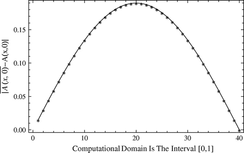
Figure 19. The absolute errors between exact and approximate solutions for $f(x)$ against the percent of noise ${\mathit{\chi }}_1={\mathit{\chi }}_2=5\%$, obtained by the Ritz-Galerkin method with $m=n=3,M=N=3$, related to Example 5.2.

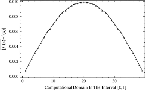
Figure 20. The absolute errors between exact and approximate solutions for $A(x,0)$ against the percent of noise ${\mathit{\chi }}_1={\mathit{\chi }}_2=5\%$, obtained by the Ritz-Galerkin method with $m=n=3,M=N=3$, related to Example 5.2.

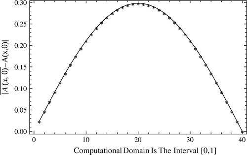
Table 3. Approximate solutions of $f(x)$ and $A(x,0)$ discussed in Example 5.2, in the presence of the different percent of noise ${\mathit{\chi }}_1={\mathit{\chi }}_2\in \{1,3,5\}\%$, obtained by the Ritz-Galerkin method with $m=n=3,M=N=3$.

$Function$	$f(x)$	$A(x,0)$	$\overline{f(x)}$	$\overline{A(x,0)}$	$\overline{f(x)}$	$\overline{A(x,0)}$	$\overline{f(x)}$	$\overline{A(x,0)}$
$x$	$Exact$	$Exact$	$1\%$	$1\%$	$3\%$	$3\%$	$5\%$	$5\%$
0.0000	0.0000	0.0000	0.0000	0.0000	0.0000	0.0000	0.0000	0.0000
0.1000	6.0997	0.3090	6.0990	0.3342	6.0978	0.3677	6.0966	0.4011
0.2000	11.6024	0.5877	11.6012	0.6357	11.5989	0.6994	11.5965	0.7631
0.3000	15.9694	0.8090	15.9678	0.8749	15.9645	0.9626	15.9613	1.0503
0.4000	18.7731	0.9510	18.7713	1.0286	18.7675	1.1316	18.7637	1.2347
0.5000	19.7392	1.0000	19.7373	1.0815	19.7333	1.1899	19.7293	1.2982
0.6000	18.7731	0.9510	18.7713	1.0286	18.7675	1.1316	18.7637	1.2347
0.7000	15.9694	0.8090	15.9678	0.8749	15.9645	0.9626	15.9613	1.0503
0.8000	11.6024	0.5877	11.6012	0.6357	11.5989	0.6994	11.5965	0.7631
0.9000	6.0997	0.3090	6.0990	0.3342	6.0978	0.3677	6.0966	0.4011
1.0000	0.0000	0.0000	0.0000	0.0000	0.0000	0.0000	0.0000	0.0000

Figure 21. The approximate solutions for $\overline{f(x)}$ against the percent of noise $\mathit{ϵ}\in \{1,3,5\}\%$ imposed to the additional data, obtained by the Ritz–Galerkin method with $k_1=k_2=k_3=1,m_1=m_2=3,m_3=2$; $\circ \circ \circ$: The exact solution,   $\bullet \bullet \bullet$: Solution when $\mathit{ϵ}=1\%$, $▽▽▽$: Solution when $\mathit{ϵ}=3\%$, $▾▾▾$: Solution when $\mathit{ϵ}=5\%$, related to Example 5.3.

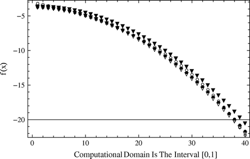
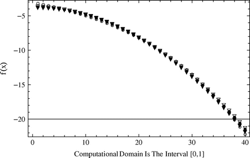
Figure 22. The approximate solutions for $\overline{f(x)}$ against the percent of noise $\mathit{ϵ}\in \{1,3,5\}\%$ imposed to the initial data, obtained by the Ritz–Galerkin method with $k_1=k_2=k_3=1,m_1=m_2=3,m_3=2$; $\circ \circ \circ$: The exact solution,   $\bullet \bullet \bullet$: Solution when $\mathit{ϵ}=1\%$,   $▽▽▽$: Solution when $\mathit{ϵ}=3\%$,   $▾▾▾$: Solution when $\mathit{ϵ}=5\%$, related to Example 5.3.

5.3 Example 3

This example,[11] illustrates the applicability of the proposed method for solving the inverse heat problem IP3 given by Equations (88 $$\begin{array}{c}\hfill \mathit{\rho }(x,t)A_t-\mathrm{\Delta }A=S(x,t),\mathrm{in}\mathrm{\Omega }\times [0,T],\end{array}$$8 ) and (99 $$\begin{array}{c}\hfill A(x,0)=A_0(x),x\in \mathrm{\Omega },\end{array}$$9 ) and (1111 $$\begin{array}{c}\hfill A(x,T)=r(x),x\in \mathrm{\Omega },\end{array}$$11 ) and (1212 $$\begin{array}{c}\hfill A(0,t)=\mathit{\phi }(t),A(1,t)=\mathit{\psi }(t),0\le t\le T,\end{array}$$12 ) with the following specifications$$\begin{array}{c}\hfill A_0(x)=exp(2x),\mathit{\phi }(t)=0,\mathit{\psi }(t)=sin(1)exp(t),r(x)=exp(2x+1),\end{array}$$$$\begin{array}{c}\hfill \mathit{\rho }(x,t)=1,g(x,t)=exp(t),h(x,t)=0,T=1.\end{array}$$With these assumptions, the problem has the exact solutions$$A(x,t)=exp(2x+t),f(x)=-3exp(2x).$$For the sake of brevity, here we only focus on the issue of the stability. First we utilize the following perturbing formula$$A^{\mathit{ϵ}}(x,1)=r^{\mathit{ϵ}}(x)=r(x)\times (1+\mathit{ϵ}\mathit{\epsilon }),$$and the following procedure solution stated in Subsection 4.3 and solving the problem in the presence of the imposed error $\mathit{ϵ}\in \{1,3,5\}\%$ we get the results depicted by Figure 21. It is clear that the fair agreement between the exact and approximate solutions holds, i.e. the numerical findings show that the errors imposed to the additional data and propagated with the approximations are of the same order.

As the last experiment we aim to study the stability with respect to the initial data. Thus again perturbing the initial condition as$$A^{\mathit{ϵ}}(x,0)=A_0^{\mathit{ϵ}}(x)=A_0(x)\times (1+\mathit{ϵ}\mathit{\epsilon }),$$and repeating the solution scheme we find the results given by Figure 22. Considering this finding we found that the stability is maintained for the solution with respect to the initial condition. Also we refer the interested reader to [58–60] for more research works on inverse parabolic problems.

6 Concluding Remarks and Future Work

Three inverse problems of reconstructing the heat source have been considered. Our study focused on providing the numerical solution for the unknown right-hand side (RHS) of the one-dimensional heat equation. The Ritz-type approximations are supposed as the solutions for the reformulated form of the IP1–IP2 and IP3 using some special observations concerning the points in space or time as additional measurements. Applying the Galerkin equations to the stated approximations, the final systems of linear equations are yielded. Since the problems are ill-posed, the optimization technique introduced in Remark 4.2 is applied to find the stable solutions. The fundamental property of the method is employing an iterative procedure known as trust region method and adjusts the trust region radius instead of adjusting the parameter of the regularization. As the consequences, we derived the solutions that possess both properties convergence and stability from the numerical point of view. Test examples given in the article obviously confirm this claim. Overall, we employed two types of basis functions for solving the problems and obtained satisfactory results as shown in numerical experiments. As the extra notifications, similar to the solution procedures given in Subsections 4.1 and 4.3 for solving IP1 and IP3 we resolved these problems using the quadrature B-spline functions, i.e. $m=2$, and found the results which are in good agreement with the exact solutions and obtained results by the Bernstein basis functions. Solution of the IP2 bears more difficulties in comparison to the two IP1 and IP3. As pointed out, considering the general possibility for the extra measurements given at $T_1<T_2<T$, we divided the domain in to three sub domains, and approximated the solution for the sub domain that includes the most initial, boundary and extra information, we used this approximation to predicting the initial data $A(x,0)$ in the sequel. The process first requires utilizing the appropriate basis to produce the robust approximation. To achieve this goal, not only we introduced the Ritz-type approximations that fulfil all the initial, boundary and extra specifications, but also the B-spline scaling functions are applied that the support of each basis is a compact sub interval. Thus the resulted final systems of equations are sparse in comparison to systems of equations related to employing the basis functions with global supports.

Also it is worth to pointing out that, care must be taken while contaminating the boundary data with the high percentage of the artificial errors. Since we use these initial and boundary data directly in the approximation, thus a strong propagation of errors can be expected especially when we impose the differential operators and as the consequence the approximation for $f(x)$ is not in agreement with the analytical solution, nor is for $A(x,0)$. It seems that recovering the accurate approximation for the initial data i.e. $\overline{A(x,0)}$ requires to set both $t=T_1$ and $t=T_2$ close to the $t=0$ as the extra observations.[23, 57] It can be expected, since considering the extra specifications as $A(x,T_s),T_s\searrow 0,s\in \{1,2\}$ and taking into account the continuation of the solution lead to apply the overdeterminations which are nearer to the $A(x,0)$ and conclude the better approximation $\overline{A(x,0)}$. On top of that, finding the accurate approximations for $A(x,0)$ is more difficult than $f(x)$, our numerical results confirm these statements and are in good adaption with previous works on the IP2.[26, 56] From the practical point of view, we can state that the proposed solutions in this paper overcome the stability for the three discussed problems. Thus we can speak of the applicability and feasibility of the new methods proposed in the current paper. Our future work will be involved studying the problems of right-hand side identification (RHS) in higher order dimensions.

Acknowledgements

The authors are very grateful to one of the reviewers for carefully reading this paper

References

- SamarskiiAA, VabishchevichAN. Numerical methods for solving inverse problems of mathematical physics. Berlin: Walter de Gruyter; 2007.
- DehghanM, YousefiSA, RashediK. Ritz-Galerkin method for solving an inverse heat conduction problem with a nonlinear source term via Bernstein multi-scaling functions and cubic B-spline functions. Inverse Probl. Sci. Eng. 2013;21:500–523.
- IsakovV. Inverse source problems. American Mathematical Society; 1990.
- CannonJR, RundellW. Recovering a time dependent coefficient in a parabolic differential equation. J. Math. Anal. Appl. 1991;160:572–582.
- DehghanM. Parameter determination in a partial differential equation from the overspecified data. Math. Comput. Model. 2005;41:196–213.
- LiaoW. A computational method to estimate the unknown coefficient in a wave equation using boundary measurements. Inverse Probl. Sci. Eng. 2011;19:855–887.
- AlifanovOM. Inverse heat transfer problems. Berlin: Springer; 1994.
- BeckJV, BlackwellB, St. ClairC. Inverse Conduction Ill-posed Problems. New York: Wiley; 1985.
- SamarskiiAA, VabishchevichAN. Computational heat transfer. Chichester: Wiley; 1995.
- BorukhovVT, VabishchevichPN. Numerical solution of the inverse problem of reconstructing a distributed right-hand side of a parabolic equation. Comput. Phys. Commun. 2000;126:32–36.
- ShidfarA, BabaeiA, MolabahramiA. Solving the inverse problem of identifying an unknown source term in a parabolic equation. Appl. Math. Comput. 2010;60:1209–1213.
- EbelA, DavitashviliT. Air water and soil quality modelling for risk and impact assessment. Dordrecht: Springer; 2007.
- KriksinYuA, PlyushchevSN, SamarskayaEA, TishkinVF. The inverse problem of source reconstruction for the equation of convective diffusion. Matematicheskoe Modelirovanie. 1995;7:95–108.
- BorukhovVT. Inversion of linear invariant in time dynamic systems with distributed parameters. Avtomatika i Telemekhanika. 1982;5:29–36.
- KryazhimskiiAV, MaksimovVI, SamarskayaYeA. Reconstruction of inputs in parabolic systems. Matematicheskoe Modelirovanie. 1997;9:51–72.
- YangL, DehghanM, YuJN, LuoGW. Inverse problem of time-dependent heat sources numerical reconstruction. Math. Comput. Simul. 2011;81:1656–1672.
- CannonJR, DuchateauP. Structural identification of an unknown source term in a heat equation. Inverse Probl. 1998;14:535–551.
- ChengW, ZhaoL, FuCL. Source term identification for an axisymmetric inverse heat conduction problem. Comput. Math. Appl. 2010;59:142–148.
- FarcasA, LesnicD. The boundary-element method for the determination of a heat source dependent on one variable. J. Engrg. Math. 2006;54:375–388.
- FatullayevAG. Numerical solution of the inverse problem of determining an unknown source term in a heat equation. Math. Comput. Simul. 2002;8:161–168.
- FatullayevAG. Numerical solution of the inverse problem of determining an unknown source term in a two-dimensional heat equation. Appl. Math. Comput. 2004;152:659–666.
- FatullayevAG, CulaS. An iterative procedure for determining an unknown spacewise-dependent coefficient in a parabolic equation. Appl. Math. Lett. 2009;22:1033–1037.
- JohanssonBT, LesnicD. An iterative boundary element method for the determination of a spacewise dependent heat source. In: GatmiriB, SellierA, AliabadiMH, editors. Advances in Boundary Element Techniques VII. UK: EC Ltd; 2006. p. 85–89.
- JohanssonBT, LesnicD. Determination of a spacewise dependent heat source. J. Comput. Appl. Math. 2007;209:66–80.
- JohanssonBT, LesnicD. A variational method for identifying a spacewise dependent heat source. IMA J. Appl. Math. 2007;72:748–760.
- JohanssonBT, LesnicD. A procedure for determining a spacewise dependent heat source and the initial temperature. Appl. Anal. 2008;87:265–276.
- MohebbiA, DehghanM. High-order scheme for determination of a control parameter in an inverse problem from the overspecified data. Comput. Phys. Commun. 2010;181:1947–1954.
- SavateevEG. On problems of determining the source function in a parabolic equation. J. Inverse Ill-Posed Probl. 1995;3:83–102.
- DehghanM, TatariM. Determination of a control parameter in a one-dimensional parabolic equation using the method of radial basis functions. Math. Comput. Model. 2006;44:1160–1168.
- DehghanM, ShakeriF. Method of lines solutions of the parabolic inverse problem with an overspecification at a point. Numer. Alg. 2009;50:417–437.
- SaadatmandiA, DehghanM. A method based on the tau approach for identification of a time-dependent coefficient in the heat equation subject to an extra measurement. J. Vibra. Control. 2012;18:1125–1132.
- ShamsiM, DehghanM. Determination of a control function in three–dimensional parabolic equations by Legendre pseudospectral method. Numer. Meth. Par. Differ. Equ. 2012;28:74–93.
- BeznoshchenkoNYa, PrilepkoAI. Inverse problems for parabolic equations. In: problems of mathematical physics and computational mathematics. Moscow: Nauka; 1977.
- SlotaD. Direct and inverse one-phase Stefan problem solved by the variational iteration method. Comput. Math. Appl. 2007;54:1139–1146.
- CannonJR, PrimicerioM. Remarks on the one-phase Stefan problem for the heat equation with the flux prescribed on the fixed boundary. J. Math. Anal. Appl. 1971;35:361–373.
- ColtonD, ReemtsenR. The numerical solution of the inverse Stefan problem in two space variables. SIAM J. Appl. Math. 1984;44:996–1013.
- ElBadiaA, MoutazaimF. A one-phase inverse Stefan problem. Inverse Probl. 1999;15:1507–1522.
- JohanssonBT, LesnicD, ReeveT. A method of fundamental solutions for the one-dimensional inverse Stefan problem. Appl. Math. Model. 2011;35:4367–4378.
- JohanssonBT, LesnicD, ReeveT. Numerical approximation of the one-dimensional inverse Cauchy–Stefan problem using a method of fundamental solutions. Invese Probl. Sci. Eng. 2011;19:659–677.
- SlotaD. Using genetic algorithms for the determination of a heat transfer coefficient in three-phase inverse Stefan problem. Int. Commun. Heat Mass Transfer. 2008;35:149–156.
- KamyninVL. The unique solvability of an inverse problem for parabolic equations under a final overdetermination condition. Math. Notes. 2003;73:202–211.
- LadyzhenskayaOA, SolonnikovVA, UraltsevaNN. Linear and quasilinear equations of parabolic type. Providence, Rhode Island: AMS; 1968.
- ShamsiM, DehghanM. Recovering a time-dependent coefficient in a parabolic equation from overspecified boundary data using the pseudospectral Legendre method. Numer. Method. Partial Differ. Equ. 2007;23:196–210.
- NevelsRD, GoswamiJC, TehraniH. Semiorthogonal wavelets basis sets for solving integral equations. IEEE Trans. Antennas. Propag. 1997;45:1332–1339.
- LakestaniM, DehghanM. Numerical solutions of the generalized Kuramoto-Sivashinsky equation using B-spline functions. Appl. Math. Model. 2012;36:605–617.
- LakestaniM, DehghanM. Numerical solution of Riccati equation using the cubic B-spline scaling functions and Chebyshev cardinal functions. Comput. Phys. Commun. 2010;181:957–966.
- LakestaniM, DehghanM. Numerical solution of Fokker-Plank equation using the cubic B-spline scaling functions. Numer. Method. Partial Differ. Equ. 2009;25:418–429.
- RashediK, AdibiH, DehghanM. Application of the Ritz-Galerkin method for recovering the spacewise-coefficients in the wave equation. Comput. Math. Appl. 2013;65:1990–2008.
- YousefiSA, BarikbinZ, DehghanM. Ritz-Galerkin method with Bernstein polynomial basis for finding the product solution form of heat equation with non-classic boundary conditions. Int. J. Numer. Methods Heat Fluid Flow. 2012;22:39–48.
- Fakhar-IzadiF, DehghanM. The spectral methods for parabolic Volterra integro-differential equations. J. Comput. Appl. Math. 2011;235:4032–4046.
- KaltenbacherB, NeubauerA, ScherzerO. Iterative regularization methods for nonlinear Ill-posed problems. Berlin: Walter de Gruyter; 2008.
- WangY, YagolaAG. Optimization and regularization for computational inverse problems and applications. Beijing: Higher Education Press; 2010.
- HansenPC. Analysis of discrete ill-posed problems by means of the L-curve. SIAM Rev. 1992;34:561–580.
- LesnicD, YousefiSA, IvanchovM. Determination of a time-dependent diffusivity from nonlocal conditions. J. Appl. Math. Comput. 2013;41:301–320.
- YousefiSA, LesnicD, BarikbinZ. Satisfier function in Ritz-Galerkin method for the identification of a time-dependent diffusivity. J. Inverse Ill-Posed Probl. 2012;20:701–722.
- MeraNS, ElliottL, InghamDB, LesnicD. An iterative boundary element method for solving the one-dimensional backward heat conduction problem. Inter. J. Heat Mass Transfer. 2001;44:1937–1946.
- LattesR, LionsJL. The method of quasi-reversibility. Applications to partial differential equations: American Elsevier Publishing, New York; 1969.
- LiaoM, DehghanM, MohebbiA. Direct numerical method for an inverse problem of a parabolic partial differential equation. J. Comput. Appl. Math. 2009;232:351–360.
- SaadatmandiA, DehghanM. Computation of two time-dependent coefficients in a parabolic partial differential equation subject to additional specifications. Intern. J. Computer Math. 2010;87:997–1008.
- LakestaniM, DehghanM. The use of Chebyshev cardinal functions for the solution of a partial differential equation with an unknown time-dependent coefficient subject to an extra measurement. J. Comput. Appl. Math. 2010;235:669–678.