Reduced forward models in electrical impedance tomography with probe geometry

Abstract

One possible technique to monitor sedimentation and froth flotation processes is electrical impedance tomography (EIT). When EIT is used in these applications, the measurements are usually conducted using a probe sensor that is positioned inside the process vessel. Full three-dimensional reconstruction is possible, however, it leads to time-consuming reconstructions. For simplifying the reconstruction procedure and reducing the computation time, two different reduced forward models are proposed. In the first model, the conductivity is considered to be rotationally symmetric, that is, the conductivity and the potential do not change in the angular direction. This model is accurate as far as the given assumptions are fulfilled. In the second model, the conductivity is considered to be invariant also in the radial direction. This one-dimensional (1D) forward model is highly approximative and therefore the reconstructed conductivity profile is useless with conventional reconstruction approach. The approximation error approach is applied to compensate the errors due to forward model reduction. The proposed approximative forward models are evaluated through computer simulations of phase interface detection showing feasible reconstructions and significant reduction in reconstruction time without compromising reconstruction accuracy.

Keywords:

• electrical impedance tomography
• probe sensor
• cylindrical symmetry
• 1D model
• approximation error

1 Introduction

In electrical impedance tomography (EIT), electrodes are typically attached on the boundary of the object and currents are injected into the object. The voltages are measured using the same electrodes and the conductivity of the object is reconstructed based on the measured voltages; for reviews on EIT, see [1–5].

In some applications, the measurements are conducted using a probe sensor that is positioned inside the process vessel. For example, in monitoring of froth flotation processes, the probe sensors could be used.[6, 7] A straightforward approach is to estimate the conductivity profile around the probe using a three-dimensional (3D) forward model. However, this approach leads to tedious computations and long computation time. Another complication is that when ring-shaped electrodes are used, the angular position of inhomogeneities cannot be reconstructed since the electrodes average the voltages in angular direction. A reasonable assumption with this type of applications and measurement configuration is that the conductivity is invariant in the angular direction. In this case, the conductivity can be modelled with two-dimensional (2D) model and it would be tempting to use computationally efficient 2D forward model. However, the conventional 2D forward model that does not take into account the cylindrical symmetry of the conductivity is very approximative model for EIT and leads to reconstruction errors when static reconstructions are computed.

Two-dimensional forward models that take into account certain symmetry of the conductivity in the boundary measurement geometry have been utilized in a few papers. In [8], it was assumed that electrodes are attached on the around the cross-sectional plane and the conductivity was assumed to be translationally invariant. The axial variation of the boundary conditions and potential field were represented using Fourier series. The 3D forward problem was solved as a succession of 2D forward problems. It was shown that this approach produced more accurate estimates of the conductivity than the approach employing conventional 2D model. This approach has been further developed in [9].

In the probe measurement geometry, the reconstruction problem is more ill-posed compared to conventional measurement geometry due to limited view of the measurements. In conventional EIT measurement setting, the measurements are conducted around the target. In the probe geometry, the measurements are conducted from linear array of electrodes and as said previously the measurements are averaged in the angular direction. The resolution of the EIT inverse problem was studied in [10] and the effect of limited-view aspect on the resolving power of the measurements was studied in [11]. In [12], the reconstruction method based on the generalized polarization tensors was studied and a numerical example of reconstruction of radially symmetric conductivity was given.

In this paper, two reduced forward models for EIT with probe geometry are proposed. In the measurement probe, the ring-shaped electrodes are used so that the measurement probe and electrodes are cylindrically symmetric. In the first model, it is assumed that the conductivity is rotationally invariant. This assumption is fairly correct in certain applications, for example, in phase interface detection in sedimentation or froth flotation process. The first forward model could also be called as cylindrically symmetric forward model. The cylindrically symmetric model is accurate model as far as the assumption of rotational invariance of the conductivity is fulfilled. This model is 2D and computationally more efficient than the full 3D model. In order to reduce the computation time further, a 1D forward model is proposed. In this model, it is assumed that the conductivity and potential change only in the vertical direction. The one-dimensional (1D) forward model is very rough and leads to significant modelling errors in the computed voltages.

The modelling errors caused by reduced forward models are compensated by using Bayesian approximation error approach which was originally proposed in [13, 14]. The key idea in the approximation error approach is, loosely speaking, to represent not only the measurement error, but also the effects of the computational model errors as an auxiliary additive noise in the observation model. The statistics of the modelling error can be computed prior to the actual image reconstruction. The statistical model of the approximation error is then used in the reconstruction process to compensate for the effect of the approximation errors. The approximation error approach was applied in EIT for discretization errors in [13, 15], truncation of computation domain in [16, 17] and unknown boundary shape in [18, 19]. It has also been applied to optical tomography to compensate errors due to unknown anisotropy,[20, 21] discretization,[22] truncation of computation domain,[23] approximative physical model [24] and nuisance parameters in the forward model,[25] for example.

In this study, the reduced forward models are evaluated with simulated examples of interface detection using EIT probe measurements. In all test cases, static (absolute) conductivity reconstructions are computed. It is shown that feasible estimates using reduced forward models can be reconstructed with significant reduction of computation time compared to the approach with full 3D model. Feasible reconstructions are also obtained with 1D approximative forward model when the approximation error approach is employed.

The rest of this paper is organized as follows. In Section 2, a brief review on the EIT electrode model is given and the weak forms for the reduced forward models are derived. In Section 3, the Bayesian formulation of the EIT problem is reviewed and the construction of the approximation error model is explained. The proposed approach is evaluated using simulated 3D EIT data in Section 4 and the conclusions are given in Section 5.

2 Forward models and notation in EIT with probe geometry

2.1 Complete electrode model

In EIT, $N_{\mathrm{el}}$ electrodes are attached on the electrode positions $e_{\ell },l=1,\dots ,N_{\mathrm{el}}$ on the boundary of the measurement probe. Using the electrodes, electric currents are injected into the body $\mathrm{\Omega }$ and corresponding voltages are measured using the same electrodes. In EIT, conductivity distribution $\mathit{\sigma }$ is estimated based on the known currents and measured voltages.

We use the complete electrode model [26, 27] as a forward model, consisting of the following equations1 $$\begin{array}{cc}\hfill \nabla ·\mathit{\sigma }(x)\nabla u(x)& =0,x\in \mathrm{\Omega }\hfill \end{array}$$1 2 $$\begin{array}{cc}\hfill u(x)+z_{\ell }\mathit{\sigma }(x)\frac{\mathit{\partial }u(x)}{\mathit{\partial }n}& =U_{\ell },x\in e_{\ell }\subset \mathit{\partial }\mathrm{\Omega },\hfill \end{array}$$2 3 $$\begin{array}{cc}\hfill {\int }_{e_{\ell }}\mathit{\sigma }(x)\frac{\mathit{\partial }u(x)}{\mathit{\partial }n}dS& =I_{\ell },x\in e_{\ell }\subset \mathit{\partial }\mathrm{\Omega },\hfill \end{array}$$3 4 $$\begin{array}{cc}\hfill \mathit{\sigma }(x)\frac{\mathit{\partial }u(x)}{\mathit{\partial }n}& =0,x\in \mathit{\partial }\mathrm{\Omega }\backslash \bigcup _{\ell =1}^{N_{\mathrm{el}}}{e}_{\ell }.\hfill \end{array}$$4 where $x\in {\mathbb{R}}^d$, $d=1,2\mathrm{o}r3$, $u(x)$ is the potential distribution inside $\mathrm{\Omega }$, $n$ is the outward unit normal vector at the boundary of the computation domain $\mathit{\partial }\mathrm{\Omega }$, $\mathit{\sigma }(x)$ is the conductivity and $z_{\ell }$ is the contact impedance between the object and the electrode $e_{\ell }$. The currents satisfy the charge conservation law5 $$\begin{array}{c}\hfill \sum _{\ell =1}^{N_{\mathrm{el}}}{I}_{\ell }=0,\end{array}$$5 and a ground level for the voltages can be fixed by6 $$\begin{array}{c}\hfill \sum _{\ell =1}^{N_{\mathrm{el}}}{U}_{\ell }=0.\end{array}$$6 Analytical solution of complete electrode model exists only in few cases. The voltages therefore have to be solved using some numerical method. In this paper, the forward problem is solved using finite element method (FEM). It has been shown that the complete electrode model has weak solution such that7 $$\begin{array}{c}\hfill B((u,U),(v,V))=\sum _{\ell =1}^{N_{\mathrm{el}}}{I}_{\ell }{V}_{\ell }\end{array}$$7 where the quadratic form is8 $$\begin{array}{c}\hfill B((u,U),(v,V))={\int }_{\mathrm{\Omega }}\mathit{\sigma }\nabla u·\nabla vdx+\sum _{\ell =1}^{N_{\mathrm{el}}}\frac{1}{z_{\ell }}{\int }_{e_{\ell }}(u-U_{\ell })(v-V_{\ell })dS.\end{array}$$8 In the FEM approximation, the domain $\mathrm{\Omega }$ is divided into $N_e$ disjoint elements joined at $N_n$ vertex nodes. The potential $u$ and electrode potentials $U\in {\mathbb{R}}^{N_{\mathrm{el}}}$ are approximated with certain basis functions. Furthermore, the conductivity is approximated with piecewise linear or piecewise constant basis functions inside each element. These approximations are substituted into the quadratic form (88 $$\begin{array}{c}\hfill B((u,U),(v,V))={\int }_{\mathrm{\Omega }}\mathit{\sigma }\nabla u·\nabla vdx+\sum _{\ell =1}^{N_{\mathrm{el}}}\frac{1}{z_{\ell }}{\int }_{e_{\ell }}(u-U_{\ell })(v-V_{\ell })dS.\end{array}$$8 ) and the resulting matrix equation is solved, see for example [28].

2.2 Reduced forward models

2.2.1 Cylindrically symmetric model

The cylindrically symmetric forward model is a tempting choice when the conductivity is rotationally invariant or when the measurements do not give information about the locations of inhomogeneities with respect to the angular coordinate. This is the case when the measurements are conducted using a measurement probe with ring-shaped electrodes.

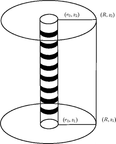
The computation domain and a schematic picture of the measurement probe are shown in Figure 1. The smaller cylinder with radius $r_0$ is the measurement probe and the larger cylinder with radius $R$ is the 3D computation domain. The 2D computation domain which is used in the cylindrically symmetric model is also shown in Figure 1.

In the rotationally symmetric case, the quadratic form (88 $$\begin{array}{c}\hfill B((u,U),(v,V))={\int }_{\mathrm{\Omega }}\mathit{\sigma }\nabla u·\nabla vdx+\sum _{\ell =1}^{N_{\mathrm{el}}}\frac{1}{z_{\ell }}{\int }_{e_{\ell }}(u-U_{\ell })(v-V_{\ell })dS.\end{array}$$8 ) is written using the cylindrical coordinates9 $$\begin{array}{cc}& B((u,U),(v,V))={\int }_{z_1}^{z_2}{\int }_0^{2\mathit{\pi }}{\int }_{r_0}^R\mathit{\sigma }\left(\frac{\mathit{\partial }u}{\mathit{\partial }r},\frac{\mathit{\partial }v}{\mathit{\partial }r},+,\frac{1}{r^2},\frac{\mathit{\partial }u}{\mathit{\partial }\mathit{\theta }},\frac{\mathit{\partial }v}{\mathit{\partial }\mathit{\theta }},+,\frac{\mathit{\partial }u}{\mathit{\partial }z},\frac{\mathit{\partial }v}{\mathit{\partial }z}\right)rdrd\mathit{\theta }dz\hfill \\ & +\sum _{\ell =1}^{N_{\mathrm{el}}}\frac{1}{z_{\ell }}{\int }_{z_{0,\ell }}^{z_{1,\ell }}{\int }_0^{2\mathit{\pi }}(u-U_{\ell })(v-V_{\ell })r_{0}d\mathit{\theta }dz,\hfill \end{array}$$9 where $z_{0,\ell }$ and $z_{1,\ell }$ are the z-coordinates of the lower and upper boundaries of the electrode $e_{\ell }$. Since the conductivity is assumed to be rotationally invariant $\mathit{\sigma }=\mathit{\sigma }(r,z)$, the potential $u$ does not change with respect to the angular coordinate $\mathit{\theta }$, that is, $\frac{\mathit{\partial }u}{\mathit{\partial }\mathit{\theta }}=0$. The quadratic form (99 $$\begin{array}{cc}& B((u,U),(v,V))={\int }_{z_1}^{z_2}{\int }_0^{2\mathit{\pi }}{\int }_{r_0}^R\mathit{\sigma }\left(\frac{\mathit{\partial }u}{\mathit{\partial }r},\frac{\mathit{\partial }v}{\mathit{\partial }r},+,\frac{1}{r^2},\frac{\mathit{\partial }u}{\mathit{\partial }\mathit{\theta }},\frac{\mathit{\partial }v}{\mathit{\partial }\mathit{\theta }},+,\frac{\mathit{\partial }u}{\mathit{\partial }z},\frac{\mathit{\partial }v}{\mathit{\partial }z}\right)rdrd\mathit{\theta }dz\hfill \\ & +\sum _{\ell =1}^{N_{\mathrm{el}}}\frac{1}{z_{\ell }}{\int }_{z_{0,\ell }}^{z_{1,\ell }}{\int }_0^{2\mathit{\pi }}(u-U_{\ell })(v-V_{\ell })r_{0}d\mathit{\theta }dz,\hfill \end{array}$$9 ) therefore reduces to10 $$\begin{array}{cc}& B((u,U),(v,V))={\int }_{z_1}^{z_2}{\int }_{r_0}^{R}2\mathit{\pi }r\mathit{\sigma }\left(\frac{\mathit{\partial }u}{\mathit{\partial }r},\frac{\mathit{\partial }v}{\mathit{\partial }r},+,\frac{\mathit{\partial }u}{\mathit{\partial }z},\frac{\mathit{\partial }v}{\mathit{\partial }z}\right)drdz\hfill \\ & +\sum _{\ell =1}^{N_{\mathrm{el}}}\frac{1}{z_{\ell }}{\int }_{z_{0,\ell }}^{z_{1,\ell }}2\mathit{\pi }{r}_0(u-U_{\ell })(v-V_{\ell })dz.\hfill \end{array}$$10 Note that when (1010 $$\begin{array}{cc}& B((u,U),(v,V))={\int }_{z_1}^{z_2}{\int }_{r_0}^{R}2\mathit{\pi }r\mathit{\sigma }\left(\frac{\mathit{\partial }u}{\mathit{\partial }r},\frac{\mathit{\partial }v}{\mathit{\partial }r},+,\frac{\mathit{\partial }u}{\mathit{\partial }z},\frac{\mathit{\partial }v}{\mathit{\partial }z}\right)drdz\hfill \\ & +\sum _{\ell =1}^{N_{\mathrm{el}}}\frac{1}{z_{\ell }}{\int }_{z_{0,\ell }}^{z_{1,\ell }}2\mathit{\pi }{r}_0(u-U_{\ell })(v-V_{\ell })dz.\hfill \end{array}$$10 ) is compared to the conventional 2D quadratic form without the cylindrical symmetry, the only difference comes from the factors $2\mathit{\pi }r$ and $2\mathit{\pi }{r}_0$ that do not exist in the conventional formulation. Thus, the implementation of the rotationally symmetric FEM requires only small changes to the conventional 2D FEM codes. This forward model is referred as the cylindrically symmetric forward model

2.2.2 1D model

To further increase the computation efficiency, a 1D forward model is derived. When the 1D forward model is derived, the conductivity is assumed to be cylindrically symmetric and also invariant in the radial direction, that is, $\mathit{\sigma }=\mathit{\sigma }(z)$. These assumptions are fairly correct in the interface detection applications. However, the potential always depends on the radial coordinate and by writing $\frac{\mathit{\partial }u}{\mathit{\partial }r}=0$ a very rough approximation is made. With this approximation (1010 $$\begin{array}{cc}& B((u,U),(v,V))={\int }_{z_1}^{z_2}{\int }_{r_0}^{R}2\mathit{\pi }r\mathit{\sigma }\left(\frac{\mathit{\partial }u}{\mathit{\partial }r},\frac{\mathit{\partial }v}{\mathit{\partial }r},+,\frac{\mathit{\partial }u}{\mathit{\partial }z},\frac{\mathit{\partial }v}{\mathit{\partial }z}\right)drdz\hfill \\ & +\sum _{\ell =1}^{N_{\mathrm{el}}}\frac{1}{z_{\ell }}{\int }_{z_{0,\ell }}^{z_{1,\ell }}2\mathit{\pi }{r}_0(u-U_{\ell })(v-V_{\ell })dz.\hfill \end{array}$$10 ) becomes11 $$\begin{array}{cc}& B((u,U),(v,V))={\int }_{z_1}^{z_2}\mathit{\pi }(R^2-r_0^2)\mathit{\sigma }\left(\frac{\mathit{\partial }u}{\mathit{\partial }z},\frac{\mathit{\partial }v}{\mathit{\partial }z}\right)dz\hfill \\ & +\sum _{\ell =1}^{N_{\mathrm{el}}}\frac{1}{z_{\ell }}{\int }_{z_{0,\ell }}^{z_{1,\ell }}2\mathit{\pi }{r}_0(u-U_{\ell })(v-V_{\ell })dz.\hfill \end{array}$$11 This forward model is referred as the 1D forward model. Note that this forward model leads to high levels of modelling error in the computed voltages. The approximation error approach is applied to compensate these modelling errors in Section 3.4.

Figure 1. A schematic picture of the measurement probe and the computation domain. The ring-shaped electrodes (black rings) are shown on the boundary of the probe. The radius of the probe $r_0=3$ cm, radius of the computation domain $R=25$ cm and height of the domain $z_2-z_1=94$ cm. The four points indicated in the figure define the rz-plane in which the 2D reconstructions are computed. Furthermore, the cross-sections of the 3D reconstructions that are shown in Section 4 are represented on the same rz-plane.

3 Bayesian approach for EIT inverse problem

In this section, Bayesian approach for the EIT inverse problem is reviewed briefly. The discussion is mainly based on [2, 13, 18, 22, 25]. For more information of the inverse problems and Bayesian framework, see [13, 29, 30] and more details on the approximation error approach, see [13, 14, 25].

In the Bayesian approach, all unknown and measured parameters are considered as random variables and the uncertainty related to their values is encoded into their probability distribution models. The joint probability density of variables $\mathit{\sigma }$ and $V$ can be written as12 $$\begin{array}{c}\hfill \mathit{\pi }(\mathit{\sigma },V)=\mathit{\pi }(\mathit{\sigma })\mathit{\pi }(V\mid \mathit{\sigma })=\mathit{\pi }(V)\mathit{\pi }(\mathit{\sigma }\mid V).\end{array}$$12 The density $\mathit{\pi }(\mathit{\sigma })$ is the prior model of the conductivity and $\mathit{\pi }(V\mid \mathit{\sigma })$ is the likelihood density, i.e. it models the probability of different measurements when the value of $\mathit{\sigma }$ is known. In the Bayesian framework, the posterior density, which is given by the Bayes formula13 $$\begin{array}{c}\hfill \mathit{\pi }(\mathit{\sigma }\mid V)=\frac{\mathit{\pi }(V\mid \mathit{\sigma })\mathit{\pi }(\mathit{\sigma })}{\mathit{\pi }(V)},\end{array}$$13 represents the complete solution of the inverse problem.

3.1 Noise model and notation

In order to solve the inverse problem in EIT, we need to have an observation model that connects the injected currents, conductivity and voltages on the electrodes. The additive Gaussian observation model is of the form14 $$\begin{array}{c}\hfill V=U_{\mathrm{\Omega }}(\mathit{\sigma })+e,e\sim \mathcal{N}(e_{}\ast ,{\mathrm{\Gamma }}_e)\end{array}$$14 where $V\in {\mathbb{R}}^m$ is the vector of the measured voltages, $U_{\mathrm{\Omega }}(\mathit{\sigma })$ is the computed voltages, $\mathrm{\Omega }$ refers to computation domain that is used, $\mathit{\sigma }\in {\mathbb{R}}^N$ and $e\in {\mathbb{R}}^m$ is a Gaussian distributed measurement noise with mean $e_{}\ast \in {\mathbb{R}}^m$ and covariance matrix ${\mathrm{\Gamma }}_e$.

3.2 Construction of the posterior model using conventional error model

If the conductivity and the noise are mutually independent, it follows from (1414 $$\begin{array}{c}\hfill V=U_{\mathrm{\Omega }}(\mathit{\sigma })+e,e\sim \mathcal{N}(e_{}\ast ,{\mathrm{\Gamma }}_e)\end{array}$$14 ) that the likelihood can be written as15 $$\begin{array}{c}\hfill \mathit{\pi }(V\mid \mathit{\sigma })={\mathit{\pi }}_e(V-U_{\mathrm{\Omega }}(\mathit{\sigma })),\end{array}$$15 where ${\mathit{\pi }}_e$ is the probability density of the noise. Moreover, if the prior model is also Gaussian, i.e. $\mathit{\sigma }\sim \mathcal{N}({\mathit{\sigma }}_{\mathrm{p}r},{\mathrm{\Gamma }}_{\mathrm{p}r})$, where ${\mathit{\sigma }}_{\mathrm{p}r}\in {\mathbb{R}}^N$ is the prior mean and ${\mathrm{\Gamma }}_{\mathrm{p}r}$ the covariance matrix of the prior, the posterior density becomes 0.0em16 $$\begin{array}{ccc}\hfill \mathit{\pi }(\mathit{\sigma }\mid V)& \hfill & \hfill {\mathit{\pi }}_{+}(\mathit{\sigma })exp\left(-,\frac{1}{2},{(V-U_{\mathrm{\Omega }}(\mathit{\sigma })-e_{}\ast )}^T,{\mathrm{\Gamma }}_e^{-1},(V-U_{\mathrm{\Omega }}(\mathit{\sigma })-e_{}\ast )\right.\\ & -\left.\frac{1}{2},{(\mathit{\sigma }-{\mathit{\sigma }}_{\mathrm{p}r})}^T,{\mathrm{\Gamma }}_{\mathrm{p}r}^{-1},(\mathit{\sigma }-{\mathit{\sigma }}_{\mathrm{p}r})\right)\hfill \end{array}$$16 where ${\mathit{\pi }}_{+}(\mathit{\sigma })$ is the positivity prior.

3.3 MAP-estimate using conventional error model

The solution is analysed and visualized by computing point estimates from the posterior density (1616 $$\begin{array}{ccc}\hfill \mathit{\pi }(\mathit{\sigma }\mid V)& \hfill & \hfill {\mathit{\pi }}_{+}(\mathit{\sigma })exp\left(-,\frac{1}{2},{(V-U_{\mathrm{\Omega }}(\mathit{\sigma })-e_{}\ast )}^T,{\mathrm{\Gamma }}_e^{-1},(V-U_{\mathrm{\Omega }}(\mathit{\sigma })-e_{}\ast )\right.\\ & -\left.\frac{1}{2},{(\mathit{\sigma }-{\mathit{\sigma }}_{\mathrm{p}r})}^T,{\mathrm{\Gamma }}_{\mathrm{p}r}^{-1},(\mathit{\sigma }-{\mathit{\sigma }}_{\mathrm{p}r})\right)\hfill \end{array}$$16 ). A common point estimate is the maximum a posteriori (MAP) estimate, which leads to the following minimization problem 0.0em17 $$\begin{array}{ccc}\hfill {\mathit{\sigma }}_{\mathrm{M}AP}& =\hfill & \hfill \mathrm{a}rg\underset{\mathit{\sigma }>0}{max}\mathit{\pi }(\mathit{\sigma }\mid V)\\ & =\hfill & \hfill \mathrm{a}rg\underset{\mathit{\sigma }>0}{min}\left\{\mid ,\mid ,L_e,(V-U_{\mathrm{\Omega }}(\mathit{\sigma })-e_{}\ast ),\mid ,{\mid }^2\right.\\ & +\left.\mid ,\mid ,L_{\mathrm{p}r},(\mathit{\sigma }-{\mathit{\sigma }}_{\mathrm{p}r}),\mid ,{\mid }^2\right\},\hfill \end{array}$$17 where $L_e$ and $L_{\mathrm{p}r}$ are Cholesky factors such that$${\mathrm{\Gamma }}_e^{-1}=L_e^T{L}_e,{\mathrm{\Gamma }}_{\mathrm{p}r}^{-1}=L_{\mathrm{p}r}^T{L}_{\mathrm{p}r}.$$The minimization problem (1717 $$\begin{array}{ccc}\hfill {\mathit{\sigma }}_{\mathrm{M}AP}& =\hfill & \hfill \mathrm{a}rg\underset{\mathit{\sigma }>0}{max}\mathit{\pi }(\mathit{\sigma }\mid V)\\ & =\hfill & \hfill \mathrm{a}rg\underset{\mathit{\sigma }>0}{min}\left\{\mid ,\mid ,L_e,(V-U_{\mathrm{\Omega }}(\mathit{\sigma })-e_{}\ast ),\mid ,{\mid }^2\right.\\ & +\left.\mid ,\mid ,L_{\mathrm{p}r},(\mathit{\sigma }-{\mathit{\sigma }}_{\mathrm{p}r}),\mid ,{\mid }^2\right\},\hfill \end{array}$$17 ) can be solved, for example, by Gauss–Newton algorithm. We refer to the solution of (1717 $$\begin{array}{ccc}\hfill {\mathit{\sigma }}_{\mathrm{M}AP}& =\hfill & \hfill \mathrm{a}rg\underset{\mathit{\sigma }>0}{max}\mathit{\pi }(\mathit{\sigma }\mid V)\\ & =\hfill & \hfill \mathrm{a}rg\underset{\mathit{\sigma }>0}{min}\left\{\mid ,\mid ,L_e,(V-U_{\mathrm{\Omega }}(\mathit{\sigma })-e_{}\ast ),\mid ,{\mid }^2\right.\\ & +\left.\mid ,\mid ,L_{\mathrm{p}r},(\mathit{\sigma }-{\mathit{\sigma }}_{\mathrm{p}r}),\mid ,{\mid }^2\right\},\hfill \end{array}$$17 ) as MAP with conventional error model (MAP-CEM).

3.4 Approximation error approach

Let us assume that a computationally sufficiently accurate measurement model can be written as18 $$\begin{array}{c}\hfill V=U_{\mathrm{\Omega }}(\overline{\mathit{\sigma }})+e,\end{array}$$18 where the FE solution of the forward problem $U_{\mathrm{\Omega }}(\overline{\mathit{\sigma }})$ is so accurate that the error in the computed voltages is smaller than the measurement error. The accurate forward problem $U_{\mathrm{\Omega }}(\overline{\mathit{\sigma }})$ is computed using the 3D forward model, that is, $\overline{\mathit{\sigma }}=\overline{\mathit{\sigma }}(r,\mathit{\theta },z)$. Furthermore, dense discretization is used to avoid discretization errors.

As explained above, in some practical applications, the measurements are conducted using a measurement probe that average the measurements in the angular direction. Furthermore, in practical applications the reconstructions have to be computed in limited time. In that case, it is tempting to use a reduced forward model (cylindrically symmetric or 1D model) to reduce the computation time. In such cases, the accurate model (1818 $$\begin{array}{c}\hfill V=U_{\mathrm{\Omega }}(\overline{\mathit{\sigma }})+e,\end{array}$$18 ) is replaced by the approximate measurement model19 $$\begin{array}{c}\hfill V\approx U_{\tilde{\mathrm{\Omega }}}(\mathit{\sigma })+e,\end{array}$$19 where $\tilde{\mathrm{\Omega }}$ refers to reduced computation domain, i.e. it is the 2D or 1D computation domain depending on which model is used. The model $U_{\tilde{\mathrm{\Omega }}}(\mathit{\sigma })$ is the model to be used in the inversion and it is referred as the target model.

3.4.1 Mappings between conductivities

The relation of representation of the conductivities $\overline{\mathit{\sigma }}$ in (1818 $$\begin{array}{c}\hfill V=U_{\mathrm{\Omega }}(\overline{\mathit{\sigma }})+e,\end{array}$$18 ) and $\mathit{\sigma }$ in (1919 $$\begin{array}{c}\hfill V\approx U_{\tilde{\mathrm{\Omega }}}(\mathit{\sigma })+e,\end{array}$$19 ) is of the form20 $$\begin{array}{c}\hfill \mathit{\sigma }(r,z)=\frac{1}{2\mathit{\pi }r}{\int }_0^{2\mathit{\pi }}\overline{\mathit{\sigma }}(r,\mathit{\theta },z)rd\mathit{\theta }=\frac{1}{2\mathit{\pi }}{\int }_0^{2\mathit{\pi }}\overline{\mathit{\sigma }}(r,\mathit{\theta },z)d\mathit{\theta }=P_{2D}\overline{\mathit{\sigma }},\end{array}$$20 when the 2D cylindrically symmetric forward model is used. The mapping $P_{2D}$ is the linear mapping $P_{2D}:\mathrm{\Omega }\mapsto \tilde{\mathrm{\Omega }}$. The relation (2020 $$\begin{array}{c}\hfill \mathit{\sigma }(r,z)=\frac{1}{2\mathit{\pi }r}{\int }_0^{2\mathit{\pi }}\overline{\mathit{\sigma }}(r,\mathit{\theta },z)rd\mathit{\theta }=\frac{1}{2\mathit{\pi }}{\int }_0^{2\mathit{\pi }}\overline{\mathit{\sigma }}(r,\mathit{\theta },z)d\mathit{\theta }=P_{2D}\overline{\mathit{\sigma }},\end{array}$$20 ) is the average value of the conductivity $\overline{\mathit{\sigma }}$ along a circular path. When the 1D forward model is used, the $\mathit{\sigma }(r,z)$ is first computed using (2020 $$\begin{array}{c}\hfill \mathit{\sigma }(r,z)=\frac{1}{2\mathit{\pi }r}{\int }_0^{2\mathit{\pi }}\overline{\mathit{\sigma }}(r,\mathit{\theta },z)rd\mathit{\theta }=\frac{1}{2\mathit{\pi }}{\int }_0^{2\mathit{\pi }}\overline{\mathit{\sigma }}(r,\mathit{\theta },z)d\mathit{\theta }=P_{2D}\overline{\mathit{\sigma }},\end{array}$$20 ) and $\mathit{\sigma }(z)$ is computed using21 $$\begin{array}{c}\hfill \mathit{\sigma }(z)=\frac{1}{R-r_0}{\int }_{r_0}^R\mathit{\sigma }(r,z)dr={\tilde{P}}_{1D}{P}_{2D}\overline{\mathit{\sigma }}=P_{1D}\overline{\mathit{\sigma }},\end{array}$$21 where ${\tilde{P}}_{1D}$ computes the average value along the radius and $P_{1D}={\tilde{P}}_{1D}{P}_{2D}$. The true mappings between the conductivities in different dimensions are unknown. However, these intuitive mappings seem to work well with the test cases considered in this paper.

3.4.2 Construction of the posterior model using approximation error approach

In the approximation error approach, instead of writing the approximation (1919 $$\begin{array}{c}\hfill V\approx U_{\tilde{\mathrm{\Omega }}}(\mathit{\sigma })+e,\end{array}$$19 ), the accurate measurement model (1818 $$\begin{array}{c}\hfill V=U_{\mathrm{\Omega }}(\overline{\mathit{\sigma }})+e,\end{array}$$18 ) is written in the form 0.0em22 $$\begin{array}{ccc}\hfill V& =\hfill & \hfill U_{\tilde{\mathrm{\Omega }}}(\mathit{\sigma })+\left(U_{\mathrm{\Omega }},(\overline{\mathit{\sigma }}),-,U_{\tilde{\mathrm{\Omega }}},(\mathit{\sigma })\right)+e\\ & =\hfill & \hfill U_{\tilde{\mathrm{\Omega }}}(\mathit{\sigma })+\mathit{\epsilon }(\overline{\mathit{\sigma }})+e\\ & =U_{\tilde{\mathrm{\Omega }}}(\mathit{\sigma })+\mathit{\eta },\hfill \end{array}$$22 where $\mathit{\epsilon }(\overline{\mathit{\sigma }})$ represents the modelling error due to approximative forward model and we denote $\mathit{\eta }=\mathit{\epsilon }(\overline{\mathit{\sigma }})+e$.

The objective in the modelling error approach is to derive a computationally efficient approximation $\tilde{\mathit{\pi }}(\mathit{\sigma }|V)$ for the posterior density $\mathit{\pi }(\mathit{\sigma }|V)$ based on the measurement model (2222 $$\begin{array}{ccc}\hfill V& =\hfill & \hfill U_{\tilde{\mathrm{\Omega }}}(\mathit{\sigma })+\left(U_{\mathrm{\Omega }},(\overline{\mathit{\sigma }}),-,U_{\tilde{\mathrm{\Omega }}},(\mathit{\sigma })\right)+e\\ & =\hfill & \hfill U_{\tilde{\mathrm{\Omega }}}(\mathit{\sigma })+\mathit{\epsilon }(\overline{\mathit{\sigma }})+e\\ & =U_{\tilde{\mathrm{\Omega }}}(\mathit{\sigma })+\mathit{\eta },\hfill \end{array}$$22 ). The posterior model corresponding to (2222 $$\begin{array}{ccc}\hfill V& =\hfill & \hfill U_{\tilde{\mathrm{\Omega }}}(\mathit{\sigma })+\left(U_{\mathrm{\Omega }},(\overline{\mathit{\sigma }}),-,U_{\tilde{\mathrm{\Omega }}},(\mathit{\sigma })\right)+e\\ & =\hfill & \hfill U_{\tilde{\mathrm{\Omega }}}(\mathit{\sigma })+\mathit{\epsilon }(\overline{\mathit{\sigma }})+e\\ & =U_{\tilde{\mathrm{\Omega }}}(\mathit{\sigma })+\mathit{\eta },\hfill \end{array}$$22 ) can be written as23 $$\begin{array}{c}\hfill \tilde{\mathit{\pi }}(\mathit{\sigma }|V)=\underset{\mathit{\pi }(V|\mathit{\sigma })}{\underbrace{{\mathit{\pi }}_{\mathit{\eta }|\mathit{\sigma }}(V-U_{\tilde{\mathrm{\Omega }}}(\mathit{\sigma })|\mathit{\sigma })}}\mathit{\pi }(\mathit{\sigma }).\end{array}$$23 see [25] for details. A complication is that the likelihood $\mathit{\pi }(V|\mathit{\sigma })$ in (2323 $$\begin{array}{c}\hfill \tilde{\mathit{\pi }}(\mathit{\sigma }|V)=\underset{\mathit{\pi }(V|\mathit{\sigma })}{\underbrace{{\mathit{\pi }}_{\mathit{\eta }|\mathit{\sigma }}(V-U_{\tilde{\mathrm{\Omega }}}(\mathit{\sigma })|\mathit{\sigma })}}\mathit{\pi }(\mathit{\sigma }).\end{array}$$23 ) does not in general have an analytic expression. To obtain a computationally feasible and efficient approximation $\tilde{\mathit{\pi }}(\mathit{\sigma }|V)$, the Gaussian approximation for the joint distribution $\mathit{\pi }(\mathit{\sigma },\mathit{\eta })$ is made. This is the core of the most common implementation of the approximation error approach, in particular, when computational efficiency is sought for. Furthermore, while it is clear that $\mathit{\epsilon }$ and $\mathit{\sigma }$ are not independent, it has turned out in several applications that a feasible approximation is obtained by approximating them to be independent. This approximation is called the enhanced error model, see [13, 14]. Then, the Gaussian approximation for the likelihood is obtained in (2323 $$\begin{array}{c}\hfill \tilde{\mathit{\pi }}(\mathit{\sigma }|V)=\underset{\mathit{\pi }(V|\mathit{\sigma })}{\underbrace{{\mathit{\pi }}_{\mathit{\eta }|\mathit{\sigma }}(V-U_{\tilde{\mathrm{\Omega }}}(\mathit{\sigma })|\mathit{\sigma })}}\mathit{\pi }(\mathit{\sigma }).\end{array}$$23 ) and the approximation for the posterior model becomes 24 $$\begin{array}{cc}\hfill \tilde{\mathit{\pi }}(\mathit{\sigma }\mid V){\mathit{\pi }}_{+}(\mathit{\sigma })& exp\left(-,\frac{1}{2},{(V-U_{\tilde{\mathrm{\Omega }}}(\mathit{\sigma })-{\mathit{\eta }}_{\ast })}^{\mathrm{T}},{\mathrm{\Gamma }}_{\mathit{\eta }}^{-1},(V-U_{\tilde{\mathrm{\Omega }}}(\mathit{\sigma })-{\mathit{\eta }}_{\ast })\right.\hfill \\ & -\left.\frac{1}{2},{(\mathit{\sigma }-{\mathit{\sigma }}_{\mathrm{p}}r)}^{\mathrm{T}},{\mathrm{\Gamma }}_{\mathrm{p}r}^{-1},(\mathit{\sigma }-{\mathit{\sigma }}_{\mathrm{p}}r)\right),\hfill \end{array}$$24 where 0.0em25 $$\begin{array}{ccc}\hfill {\mathit{\eta }}_{\ast }& =\hfill & \hfill {\mathit{\epsilon }}_{}\ast +e_{}\ast \end{array}$$25 26 $$\begin{array}{ccc}\hfill {\mathrm{\Gamma }}_{\mathit{\eta }}& =\hfill & \hfill {\mathrm{\Gamma }}_{\mathit{\epsilon }}+{\mathrm{\Gamma }}_e.\end{array}$$26 Note that in the case of non-linear forward models, the mean ${\mathit{\epsilon }}_{}\ast$ and the covariance ${\mathrm{\Gamma }}_{\mathit{\epsilon }}$, in Equations (2525 $$\begin{array}{ccc}\hfill {\mathit{\eta }}_{\ast }& =\hfill & \hfill {\mathit{\epsilon }}_{}\ast +e_{}\ast \end{array}$$25 )–(2626 $$\begin{array}{ccc}\hfill {\mathrm{\Gamma }}_{\mathit{\eta }}& =\hfill & \hfill {\mathrm{\Gamma }}_{\mathit{\epsilon }}+{\mathrm{\Gamma }}_e.\end{array}$$26 ) need to be estimated based on Monte Carlo simulations. However, this task can be done offline and needs to be done only once for a given measurement set-up, and for the expected range of uncertainties.

3.4.3 MAP-estimate with approximation error model

The computation of the MAP estimate from the posterior model (2424 $$\begin{array}{cc}\hfill \tilde{\mathit{\pi }}(\mathit{\sigma }\mid V){\mathit{\pi }}_{+}(\mathit{\sigma })& exp\left(-,\frac{1}{2},{(V-U_{\tilde{\mathrm{\Omega }}}(\mathit{\sigma })-{\mathit{\eta }}_{\ast })}^{\mathrm{T}},{\mathrm{\Gamma }}_{\mathit{\eta }}^{-1},(V-U_{\tilde{\mathrm{\Omega }}}(\mathit{\sigma })-{\mathit{\eta }}_{\ast })\right.\hfill \\ & -\left.\frac{1}{2},{(\mathit{\sigma }-{\mathit{\sigma }}_{\mathrm{p}}r)}^{\mathrm{T}},{\mathrm{\Gamma }}_{\mathrm{p}r}^{-1},(\mathit{\sigma }-{\mathit{\sigma }}_{\mathrm{p}}r)\right),\hfill \end{array}$$24 ) amounts to solving the minimization problem 0.0em27 $$\begin{array}{ccc}\hfill {\mathit{\sigma }}_{\mathrm{M}AP}& =\hfill & \hfill \mathrm{a}rg\underset{\mathit{\sigma }>0}{min}\left\{\mid ,\mid ,L_{\mathit{\eta }},(V-U_{\tilde{\mathrm{\Omega }}}(\mathit{\sigma })-{\mathit{\eta }}_{\ast }),\mid ,{\mid }^2\right.\\ & +\left.\mid ,\mid ,L_{\mathrm{p}r},(\mathit{\sigma }-{\mathit{\sigma }}_{\mathrm{p}}r),\mid ,{\mid }^2\right\},\hfill \end{array}$$27 where the Cholesky factor $L_{\mathit{\eta }}^{\mathrm{T}}{L}_{\mathit{\eta }}={\mathrm{\Gamma }}_{\mathit{\eta }}^{-1}$. Thus, the MAP estimation problem with the modelling error approach is formally similar to the MAP estimation (1717 $$\begin{array}{ccc}\hfill {\mathit{\sigma }}_{\mathrm{M}AP}& =\hfill & \hfill \mathrm{a}rg\underset{\mathit{\sigma }>0}{max}\mathit{\pi }(\mathit{\sigma }\mid V)\\ & =\hfill & \hfill \mathrm{a}rg\underset{\mathit{\sigma }>0}{min}\left\{\mid ,\mid ,L_e,(V-U_{\mathrm{\Omega }}(\mathit{\sigma })-e_{}\ast ),\mid ,{\mid }^2\right.\\ & +\left.\mid ,\mid ,L_{\mathrm{p}r},(\mathit{\sigma }-{\mathit{\sigma }}_{\mathrm{p}r}),\mid ,{\mid }^2\right\},\hfill \end{array}$$17 ) with the conventional noise model, and therefore the functional (2727 $$\begin{array}{ccc}\hfill {\mathit{\sigma }}_{\mathrm{M}AP}& =\hfill & \hfill \mathrm{a}rg\underset{\mathit{\sigma }>0}{min}\left\{\mid ,\mid ,L_{\mathit{\eta }},(V-U_{\tilde{\mathrm{\Omega }}}(\mathit{\sigma })-{\mathit{\eta }}_{\ast }),\mid ,{\mid }^2\right.\\ & +\left.\mid ,\mid ,L_{\mathrm{p}r},(\mathit{\sigma }-{\mathit{\sigma }}_{\mathrm{p}}r),\mid ,{\mid }^2\right\},\hfill \end{array}$$27 ) can be minimized with the same algorithms as the MAP with conventional noise model (1717 $$\begin{array}{ccc}\hfill {\mathit{\sigma }}_{\mathrm{M}AP}& =\hfill & \hfill \mathrm{a}rg\underset{\mathit{\sigma }>0}{max}\mathit{\pi }(\mathit{\sigma }\mid V)\\ & =\hfill & \hfill \mathrm{a}rg\underset{\mathit{\sigma }>0}{min}\left\{\mid ,\mid ,L_e,(V-U_{\mathrm{\Omega }}(\mathit{\sigma })-e_{}\ast ),\mid ,{\mid }^2\right.\\ & +\left.\mid ,\mid ,L_{\mathrm{p}r},(\mathit{\sigma }-{\mathit{\sigma }}_{\mathrm{p}r}),\mid ,{\mid }^2\right\},\hfill \end{array}$$17 ). We refer to the MAP estimate (2727 $$\begin{array}{ccc}\hfill {\mathit{\sigma }}_{\mathrm{M}AP}& =\hfill & \hfill \mathrm{a}rg\underset{\mathit{\sigma }>0}{min}\left\{\mid ,\mid ,L_{\mathit{\eta }},(V-U_{\tilde{\mathrm{\Omega }}}(\mathit{\sigma })-{\mathit{\eta }}_{\ast }),\mid ,{\mid }^2\right.\\ & +\left.\mid ,\mid ,L_{\mathrm{p}r},(\mathit{\sigma }-{\mathit{\sigma }}_{\mathrm{p}}r),\mid ,{\mid }^2\right\},\hfill \end{array}$$27 ) as MAP with the approximation error model (MAP-AEM).

3.4.4 Computation of the statistics of the approximation error

In cases in which the measurement model is linear and the prior model is Gaussian, the approximation error statistics can be computed analytically, see [13]. The statistics is, however, typically estimated by Monte Carlo simulation by simulating samples from the prior model and computing the difference between forward solutions using ‘accurate’ and ‘inaccurate’ model. Note that the prior model used for the generation of the samples does not have to be the same model that is used in the inversion. Furthermore, closed form representation for the prior is not necessarily needed.

For the Monte Carlo simulation, a set of $N_S=2000$ samples $\{{\overline{\mathit{\sigma }}}^{(\ell )},\ell =1,2,\dots ,2000\}$ were generated. These samples were then used for the computation of the accurate forward solution $U_{\mathrm{\Omega }}({\overline{\mathit{\sigma }}}^{(\ell )})$ and for the target model solution $U_{\tilde{\mathrm{\Omega }}}(P{\overline{\mathit{\sigma }}}^{(\ell )})$ for each of the $N_s$ samples. The conductivity samples were mapped from $\mathrm{\Omega }\subset {\mathbb{R}}^3$ to model domain $\tilde{\mathrm{\Omega }}\subset {\mathbb{R}}^{1,2}$ by$${\mathit{\sigma }}^{(\ell )}=P{\overline{\mathit{\sigma }}}^{(\ell )},P:\mathrm{\Omega }\mapsto ,\tilde{\mathrm{\Omega }}$$where $P$ is a matrix that represents the mapping (2020 $$\begin{array}{c}\hfill \mathit{\sigma }(r,z)=\frac{1}{2\mathit{\pi }r}{\int }_0^{2\mathit{\pi }}\overline{\mathit{\sigma }}(r,\mathit{\theta },z)rd\mathit{\theta }=\frac{1}{2\mathit{\pi }}{\int }_0^{2\mathit{\pi }}\overline{\mathit{\sigma }}(r,\mathit{\theta },z)d\mathit{\theta }=P_{2D}\overline{\mathit{\sigma }},\end{array}$$20 ) or (2121 $$\begin{array}{c}\hfill \mathit{\sigma }(z)=\frac{1}{R-r_0}{\int }_{r_0}^R\mathit{\sigma }(r,z)dr={\tilde{P}}_{1D}{P}_{2D}\overline{\mathit{\sigma }}=P_{1D}\overline{\mathit{\sigma }},\end{array}$$21 ).

The 3D conductivity samples $\{{\overline{\mathit{\sigma }}}^{(\ell )},\ell =1,2,\dots ,N_s\}$ were randomly generated. The aim was to generate typical conductivities in the phase interface detection application. The conductivity is modelled to be homogeneous in the upper and bottom parts of the computation domain and there is a smooth transition (phase interface) at a random height. This type of conductivity is typical, for example, in the froth flotation when the froth and slurry have different conductivities and the location of the froth slurry interface is unknown. The location of the interface is denoted by $z=z_{\mathrm{j}ump}$ (cm) and the conductivities of the lower and upper parts ${\mathit{\sigma }}_{\mathrm{d}own}$ and ${\mathit{\sigma }}_{\mathrm{u}p}$, correspondingly. The location of the interface was drawn from a uniform distribution $z_{\mathrm{j}ump}\sim \mathcal{U}(0,94)$ (the height of the probe is 94 cm), that is, no prior information was assumed on the location. The conductivities ${\mathit{\sigma }}_{\mathrm{u}p}$ and ${\mathit{\sigma }}_{\mathrm{d}own}$ were modelled with independent Gaussian distributions ${\mathit{\sigma }}_{\mathrm{u}p}\sim \mathcal{N}(4.61,2^2)$ and ${\mathit{\sigma }}_{\mathrm{d}own}\sim \mathcal{N}(4.61,2^2)$. Note that the prior density of the conductivity should be chosen so that the prior density covers well the expected range of conductivities. Furthermore, other than this, Gaussian densities can be used as well, see for example [17]. Given the accurate and target forward solutions, the samples ${\mathit{\epsilon }}^{(\ell )}$ of the approximation error were obtained as$${\mathit{\epsilon }}^{(\ell )}=U_{\mathrm{\Omega }}({\overline{\mathit{\sigma }}}^{(\ell )})-U_{\tilde{\mathrm{\Omega }}}({\mathit{\sigma }}^{(\ell )})$$The second-order statistics of the modelling error was then estimated as$${\mathit{\epsilon }}_{\ast }=\frac{1}{N_s}\sum _{\ell =1}^{N_s}{\mathit{\epsilon }}^{(\ell )},{\mathrm{\Gamma }}_{\mathit{\epsilon }}=\frac{1}{N_s-1}\sum _{\ell =1}^{N_s}{\mathit{\zeta }}^{(\ell )}{{\mathit{\zeta }}^{(\ell )}}^{\mathrm{T}},$$where ${\mathit{\zeta }}^{(\ell )}={\mathit{\epsilon }}^{(\ell )}-{\mathit{\epsilon }}_{\ast }$, and the Gaussian approximation $\mathit{\pi }(\mathit{\epsilon })\approx \mathcal{N}({\mathit{\epsilon }}_{\ast },{\mathrm{\Gamma }}_{\mathit{\epsilon }})$ was written.

3.5 Prior model

The Gaussian smoothness prior model $\mathit{\sigma }\sim \mathcal{N}({\mathit{\sigma }}_{\mathrm{p}}r,{\mathrm{\Gamma }}_{\mathrm{p}}r)$ was used in all test cases in inverse computations. The prior used in here is a modification of the Gaussian smoothness priors represented in [13, 31]. For the construction of the prior, the conductivity is written in the form$$\mathit{\sigma }(x)={\mathit{\sigma }}_{\mathrm{in}}(x)+{\mathit{\sigma }}_{\mathrm{hg}}(x)$$where ${\mathit{\sigma }}_{\mathrm{in}}(x)$ is a spatially inhomogeneous conductivity with zero mean and ${\mathit{\sigma }}_{\mathrm{hg}}(x)$ is a spatially homogeneous conductivity of non-zero mean. The homogeneous part is of the form ${\mathit{\sigma }}_{\mathrm{hg}}(x)=c\mathbb{I}$, where $\mathbb{I}\in {\mathbb{R}}^N$ is a vector of ones and $\mathbb{R}\ni c\sim \mathcal{N}({\mathit{\sigma }}_{\mathrm{p}}r,{\mathit{\mu }}_{\mathrm{hg}}^2)$. The inhomogeneous part of the conductivity is modelled as ${\mathit{\sigma }}_{\mathrm{in}}\sim \mathcal{N}(0,{\mathrm{\Gamma }}_{\mathrm{in}})$. The conductivities ${\mathit{\sigma }}_{\mathrm{in}}$ and $c$ are modelled as mutually independent, that is, with respect to the prior model, the background conductivity is modelled mutually independent with the inhomogeneities in the conductivity. The prior covariance matrix is of the form ${\mathrm{\Gamma }}_{\mathrm{p}}r={\mathrm{\Gamma }}_{\mathrm{i}}n+{\mathit{\mu }}_{\mathrm{h}}{g}^2\mathbb{I}{\mathbb{I}}^{\mathrm{T}}$.

The covariance matrix is written as28 $$\begin{array}{c}\hfill {\mathrm{\Gamma }}_{\mathrm{p}}r(i,j)=aexp\left\{-,\sum _{k=1}^{\mathrm{d}im},\frac{{(x_k^i-x_k^j)}^2}{2{\mathit{\beta }}_k^2}\right\}+{\mathit{\mu }}_{\mathrm{hg}}^2={\mathrm{\Gamma }}_{\mathrm{i}}n(i,j)+{\mathrm{\Gamma }}_{\mathrm{h}}g(i,j),\end{array}$$28 where the covariance matrix is split to the inhomogeneous part ${\mathrm{\Gamma }}_{\mathrm{i}}n$ and homogeneous part ${\mathrm{\Gamma }}_{\mathrm{h}}g$. The correlation between discretized conductivities ${\mathit{\sigma }}_i$ and ${\mathit{\sigma }}_j$ depends on the corresponding Euclidean distance between the coordinate points $x_k^i$ and $x_k^j$. The parameter $\mathrm{d}im=1,2\mathrm{o}r3$ is the dimension of the coordinate system. The tuning parameters of the model are the variance $a$, the correlation length ${\mathit{\beta }}_k$ and ${\mathit{\mu }}_{\mathrm{hg}}\in \mathbb{R}$, the standard deviation of the homogeneous part of the conductivity. The anisotropic smoothness prior can be constructed by tuning ${\mathit{\beta }}_k$ for every $k$. Note that in 3D, the notation $\mathit{\beta }=({\mathit{\beta }}_1,{\mathit{\beta }}_2,{\mathit{\beta }}_3)=({\mathit{\beta }}_{\mathrm{x}},{\mathit{\beta }}_{\mathrm{y}},{\mathit{\beta }}_{\mathrm{z}})$ is used and in 2D and 1D notations $\mathit{\beta }=({\mathit{\beta }}_1,{\mathit{\beta }}_2)=({\mathit{\beta }}_{\mathrm{r}},{\mathit{\beta }}_{\mathrm{z}})$ and $\mathit{\beta }=({\mathit{\beta }}_1)=({\mathit{\beta }}_{\mathrm{z}})$ are used.

By using this formalism, it is possible to model some regions inside the computation domain to be purely homogeneous. The computation domain $\mathrm{\Omega }$ is divided to the (assumed) homogeneous part ${\mathrm{\Omega }}_2$ and inhomogeneous part ${\mathrm{\Omega }}_1$. This approach is used to correct errors in the 1D reconstruction at the top and bottom ends of the measurement probe. At the ends of the probe, there is an electrode-free region where the reconstructions are usually erroneous. The homogeneous parts are separated with dotted lines in Figure 2.

The covariance matrix is now of the form29 $$\begin{array}{c}\hfill {\mathrm{\Gamma }}_{\mathrm{p}}r(i,j)=\left\{\begin{array}{cc}\hfill aexp\left\{-,\sum _{k=1}^{\mathrm{d}im},\frac{{\left(x_k^i,-,x_k^j\right)}^2}{2{\mathit{\beta }}_k^2}\right\}+{\mathit{\mu }}_{\mathrm{hg}}^2& ,\forall x_k^i,x_k^j\in {\mathrm{\Omega }}_1,\hfill \\ \hfill {\mathit{\mu }}_{\mathrm{hg}}^2& ,\forall x_k^i,x_k^j\in {\mathrm{\Omega }}_2,\hfill \\ \hfill aexp\left\{-,\sum _{k=1}^{\mathrm{d}im},\frac{{\left(x_k^i,-,x_k^l\right)}^2}{2{\mathit{\beta }}_k^2}\right\}+{\mathit{\mu }}_{\mathrm{hg}}^2& ,\forall x_k^i\in {\mathrm{\Omega }}_1,x_k^j\in {\mathrm{\Omega }}_2.\hfill \end{array}\right.\end{array}$$29 where30 $$\begin{array}{c}\hfill x_k^l=\underset{x_k^j}{min}|x_k^i-x_k^j|,x_k^i\in {\mathrm{\Omega }}_1,x_k^j\in {\mathrm{\Omega }}_2.\end{array}$$30 That is the point $x_k^l$ is chosen from ${\mathrm{\Omega }}_2$ so that the distance to point $x_k^i$ is minimized.

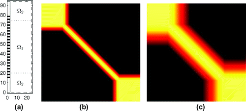
The covariance matrix for the 1D problem computed with the above method is shown in Figure 2. The elements (line segments) are indexed so that the first element is located on the bottom and the last element is on the top of the computation domain. The homogeneous parts of the computation domain can be seen in the covariance matrix as block type structures. The correlation length is ${\mathit{\beta }}_{\mathrm{z}}=5$ cm in Figure 2(b) and ${\mathit{\beta }}_{\mathrm{z}}=15$ cm in Figure 2(c).

Figure 2. (a) The computation domain and the measurement probe. The electrodes are shown with black patches. In some inverse solutions, the conductivity is assumed to be homogeneous in the upper and bottom parts of the computation domain. The cutting planes of the homogeneous parts are shown with dashed horizontal lines (location in the $z$-axis is $z=20$ and $z=74$). (b) A prior covariance matrix for 1D reconstructions (correlation length ${\mathit{\beta }}_{\mathrm{z}}=5$ cm and variance $a=1000$). (c) A prior covariance matrix for 1D reconstructions (correlation length ${\mathit{\beta }}_{\mathrm{z}}=15$ cm and variance $a=1000$).

4 Image reconstructions

4.1 Estimates and computation domains

All estimates were computed using Gauss–Newton iteration and the same stopping criterion was used in all computations. When the MAP-CEM estimate is computed the Gauss–Newton iteration is of the form31 $$\begin{array}{c}\hfill {\mathit{\sigma }}_{i+1}={\mathit{\sigma }}_i+{(J^{\mathrm{T}}{\mathrm{\Gamma }}_e^{-1}J+{\mathrm{\Gamma }}_{\mathrm{p}}{r}^{-1})}^{-1}\left(J^{\mathrm{T}},{\mathrm{\Gamma }}_e^{-1},(V-U_{\mathrm{\Omega }}({\mathit{\sigma }}_i)-e_{}\ast ),-,{\mathrm{\Gamma }}_{\mathrm{p}},r^{-1},({\mathit{\sigma }}_i-{\mathit{\sigma }}_{\mathrm{p}}r)\right),\end{array}$$31 where $J=J({\mathit{\sigma }}_i)$ is the Jacobian matrix. When the MAP-AEM estimate is computed the Gauss–Newton iteration is of the form32 $$\begin{array}{c}\hfill {\mathit{\sigma }}_{i+1}={\mathit{\sigma }}_i+{\left(J^{\mathrm{T}},{\mathrm{\Gamma }}_{\mathit{\eta }}^{-1},J,+,{\mathrm{\Gamma }}_{\mathrm{p}},r^{-1}\right)}^{-1}\left(J^{\mathrm{T}},{\mathrm{\Gamma }}_{\mathit{\eta }}^{-1},(V-U_{\tilde{\mathrm{\Omega }}}({\mathit{\sigma }}_i)-{\mathit{\eta }}_{}\ast ),-,{\mathrm{\Gamma }}_{\mathrm{p}},r^{-1},({\mathit{\sigma }}_i-{\mathit{\sigma }}_{\mathrm{p}}r)\right).\end{array}$$32 The starting point of the iteration ${\mathit{\sigma }}_0$ is the mean of the prior density ${\mathit{\sigma }}_0={\mathit{\sigma }}_{\mathrm{p}}r=4.61$. The correct values of the contact impedances are used, that is, the contact impedances used in the simulation of the measurements are used also in the inverse problem. The contact impedances were $z_{\ell }=0.1$.

The results were computed with different correlation lengths in the prior model (the values are given in Section 4). Based on the simulation tests, the variances of the inhomogeneous part $a$ and homogeneous part ${\mathit{\mu }}_{\mathrm{h}}{g}^2$ have to be different with 1D model compared to 3D and 2D models. In 3D and 2D reconstruction, problems variances were $a=2$ and ${\mathit{\mu }}_{\mathrm{h}}{g}^2=0$. In 1D reconstruction, problems variances were $a=1000$ and ${\mathit{\mu }}_{\mathrm{h}}{g}^2=1$. The values of the variances were found by visual inspection.

The proposed reduced forward models were applied for the simulated test cases of phase interface detection. The following type of estimates were computed.

(1)	MAP-AEM estimate with 3D computation domain using coarse discretization. In this case, the approximation error approach is applied to compensate the discretization errors. The coarse discretization is used to reduce the computation time. The approximation error approach has been applied by several authors for compensating discretization errors, see [13, 22] for details. Furthermore, the mean vertical conductivity profile is also computed using (2121 $$\begin{array}{c}\hfill \mathit{\sigma }(z)=\frac{1}{R-r_0}{\int }_{r_0}^R\mathit{\sigma }(r,z)dr={\tilde{P}}_{1D}{P}_{2D}\overline{\mathit{\sigma }}=P_{1D}\overline{\mathit{\sigma }},\end{array}$$21 ). This estimate is referred to full 3D reconstruction.
(2)	MAP-REF estimate in which the forward problems are solved using 3D model but the inverse problem is solved using 1D model for the conductivity. The idea of the approach is to divide the 3D computation domain into horizontal layers and model the conductivity to be homogeneous inside these layers. The Gauss–Newton iteration (3131 $$\begin{array}{c}\hfill {\mathit{\sigma }}_{i+1}={\mathit{\sigma }}_i+{(J^{\mathrm{T}}{\mathrm{\Gamma }}_e^{-1}J+{\mathrm{\Gamma }}_{\mathrm{p}}{r}^{-1})}^{-1}\left(J^{\mathrm{T}},{\mathrm{\Gamma }}_e^{-1},(V-U_{\mathrm{\Omega }}({\mathit{\sigma }}_i)-e_{}\ast ),-,{\mathrm{\Gamma }}_{\mathrm{p}},r^{-1},({\mathit{\sigma }}_i-{\mathit{\sigma }}_{\mathrm{p}}r)\right),\end{array}$$31 ) is modified so that the conductivity inside these layers is estimated. The indexes of the nodes in each layer (when linear basis functions for conductivity is used) are denoted as $\mathrm{i}n{d}_i,i=1,2,\dots ,n$, where $n$ is the number of layers. The new Jacobian matrix is computed as follows: $i$:th column of Jacobian $J_{1}D(:,i)$ is the sum of columns of 3D Jacobian: $J_{1}D(:,i)=\mathrm{s}um(J(:,\mathrm{i}n{d}_i))$. Similar type of approach is also used in [6, 7]. Note that this approach is computationally expensive since the forward problems and Jacobian matrix are computed using 3D model. This estimate is referred to 3D/1D reconstructions.
(3)	MAP-AEM estimate using 2D cylindrically symmetric model. In this estimate, the approximation error between the accurate 3D model and 2D cylindrically symmetric model is compensated using approximation error approach. Furthermore, the mean vertical conductivity profile is also computed using (2020 $$\begin{array}{c}\hfill \mathit{\sigma }(r,z)=\frac{1}{2\mathit{\pi }r}{\int }_0^{2\mathit{\pi }}\overline{\mathit{\sigma }}(r,\mathit{\theta },z)rd\mathit{\theta }=\frac{1}{2\mathit{\pi }}{\int }_0^{2\mathit{\pi }}\overline{\mathit{\sigma }}(r,\mathit{\theta },z)d\mathit{\theta }=P_{2D}\overline{\mathit{\sigma }},\end{array}$$20 ).This estimate is referred to 2D reconstruction.
(4)	MAP-AEM estimate using 1D forward model. In this estimate, the approximation error between the accurate 3D model and 1D model is compensated using approximation error approach. These estimates are computed using the Gaussian smoothness prior presented in Section 3.5. Two types of estimates are computed either assuming the homogeneity at both ends of the computation domain or without this assumption. This estimate is referred to 1D reconstruction.
(5)	MAP-CEM estimate using 1D forward model. These estimates are computed using the Gaussian smoothness prior presented in Section 3.5. Two types of estimates are computed either assuming the homogeneity at both ends of the computation domain or without this assumption. This estimate is referred to 1D MAP-CEM.

The feasibility of the estimates was evaluated by computing the relative estimation errors33 $$\begin{array}{c}\hfill {\mathrm{\Delta }}_{\mathit{\sigma }}=\frac{\mid \mid P_{1}D{\mathit{\sigma }}_{\mathrm{t}}rue-P_i{\mathit{\sigma }}_{\mathrm{M}AP}\mid \mid }{\mid \mid P_{1}D{\mathit{\sigma }}_{\mathrm{t}}rue\mid \mid }\times 100\%,\end{array}$$33 where ${\mathit{\sigma }}_{\mathrm{t}}rue$ is the true simulated 3D conductivity, $P_{1}D$ is mapping (2121 $$\begin{array}{c}\hfill \mathit{\sigma }(z)=\frac{1}{R-r_0}{\int }_{r_0}^R\mathit{\sigma }(r,z)dr={\tilde{P}}_{1D}{P}_{2D}\overline{\mathit{\sigma }}=P_{1D}\overline{\mathit{\sigma }},\end{array}$$21 ) and $P_i$ is mapping (2121 $$\begin{array}{c}\hfill \mathit{\sigma }(z)=\frac{1}{R-r_0}{\int }_{r_0}^R\mathit{\sigma }(r,z)dr={\tilde{P}}_{1D}{P}_{2D}\overline{\mathit{\sigma }}=P_{1D}\overline{\mathit{\sigma }},\end{array}$$21 ) for 3D reconstruction, mapping in (2020 $$\begin{array}{c}\hfill \mathit{\sigma }(r,z)=\frac{1}{2\mathit{\pi }r}{\int }_0^{2\mathit{\pi }}\overline{\mathit{\sigma }}(r,\mathit{\theta },z)rd\mathit{\theta }=\frac{1}{2\mathit{\pi }}{\int }_0^{2\mathit{\pi }}\overline{\mathit{\sigma }}(r,\mathit{\theta },z)d\mathit{\theta }=P_{2D}\overline{\mathit{\sigma }},\end{array}$$20 ) for 2D reconstruction and identity matrix for 1D reconstructions.

The 3D computation domain is shown in Figure 1. The radius and height of the computation domain are $R=25$ cm and 94 cm, respectively. The measurement probe, the arrangement of the electrodes (number of electrodes is 22) and 2D computation domain are shown in Figure 2. The radius of the measurement probe is $r_0=3$. The height of the electrodes is 1 cm and the space between every electrode is 2 cm. At both ends of the measurement probe, there is 15 cm of electrode-free space. The 1D computation domain is 94 cm long line where the electrodes are modelled as 1 cm long line segments.

Figure 3. Simulated conductivities used for the simulation of the measurements.

4.2 Target conductivities and simulation of measurements

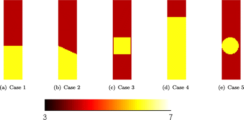
The cross-sections of the simulated 3D target conductivities for Cases 1–5 are shown in Figure 3. The cross-sections that are shown are from 2D plane that is defined using four corner points in Figure 1. The conductivities in Cases 1–4 are rotationally symmetric. In Case 5, the middle cross-section of a sphere with radius of 10 cm inside the homogeneous background is shown. Thus, the Case 5 represents a difficult case since the assumption of the cylindrical symmetry of the conductivity is violated. Note that the conductivity distributions in Case 3 and 5 are not realistic in flotation and sedimentation applications. These cases were chosen to evaluate the ability of the proposed approaches to locate phase interfaces in more complicated cases and also in a case when the conductivity violates the symmetry assumptions (Case 5). The conductivities in Cases 1 and 4 depend only on the vertical axis ($z$-axis). The reconstruction of the conductivity in Case 4 is expected to be more difficult than in Case 1 because the simulated phase interface in Case 4 is near the end of the electrode arrangement (between the 2. and 3. electrode).

The measurements were simulated using current injections between all adjacent pairs and one injection between the first and last electrodes. The voltages were measured using the same pairs of electrodes that were used for current injection leading to $22\times 22=484$ voltage measurements. When reconstructions were computed using 1D forward model, only measurements corresponding to current injection between the first and last electrodes were used. The measurements were computed using a mesh ${\mathcal{M}}_{\mathrm{s}im}$ that is denser than a mesh ${\mathcal{M}}_{3D}$ in order to prevent inverse crime (see Table 1). Furthermore, Gaussian mutually independent noise was added to the simulated voltages. The mean of the noise was zero and the standard deviation was 0.1% of the computed simulated voltages, i.e. ${(\mathrm{d}iag({\mathrm{\Gamma }}_e))}^{1/2}/U(\mathit{\sigma })\times 100\%=0.1\%$.

Table 1. Finite element meshes, where $N_n$ is the number of nodes, $N_e$ the number of elements in meshes and basis is the basis functions used for the conductivity.

Mesh	$N_n$	$N_e$	Basis	Usage
${\mathcal{M}}_{\mathrm{s}im}$	72,484	365,977	Linear	Simulation of measurements
${\mathcal{M}}_{3D}$	33,225	167,928	Linear	3D model
${\mathcal{M}}_{3D,\mathrm{i}nv}$	3448	16,170	Linear	3D inversion
${\mathcal{M}}_{2D}$	2280	4324	Constant	2D model
${\mathcal{M}}_{1D}$	941	940	Constant	1D model

The details of the meshes are listed in Table 1. For the 3D computations, three different meshes are used. As mentioned previously, ${\mathcal{M}}_{\mathrm{s}im}$ is used for the simulation of the measurements. The mesh ${\mathcal{M}}_{3D,\mathrm{i}nv}$ is used in the inverse problem and ${\mathcal{M}}_{3D}$ is used for the ‘accurate’ forward problem solutions in the estimation of the modelling error statistics. The computations of the 3D inverse problems were conducted using coarse mesh ${\mathcal{M}}_{3D,\mathrm{i}nv}$ to reduce the computation time.

4.3 Forward simulation tests

The simulated voltages in Case 1 are shown in Figure 4. The voltages are shown without added noise. The location of the simulated phase interface is between the 13. and 14. electrodes. As can be seen, the voltages corresponding to 3D and 2D cylindrically symmetric model are very similar as expected since the conductivity profile is cylindrically symmetric and therefore the assumptions are fulfilled. The voltage drop between the 13. and 14. electrodes is clearly visible. The difference between the computed voltages is due to discretization and different basis functions used for the conductivity. The voltages computed with the 1D forward model are highly erroneous. These errors are due to approximations made in the derivation of the model. Furthermore, the 1D model cannot model the current flow in the real 3D target. The voltage drop due to the phase interface is visible also in the voltages computed with the 1D model.

Figure 4. The simulated voltages for the Case 1. (a) All simulated voltages corresponding to current injection between the first and last electrodes are shown. (b) Only the voltages measured near the interface in the conductivity are shown. The voltages shown with blue (thick line), red (thin line) and black (dashed line) are computed with 3D, 2D and 1D models, respectively.

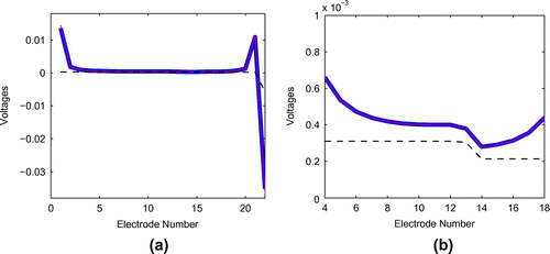
Figure 5. (a) The average percentual modelling error level between 3D and 1D model. (b) The average percentual modelling error level between 3D and 2D cylindrically symmetric model. The mean is shown with blue line and standard deviation with thick red line.

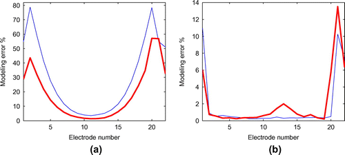
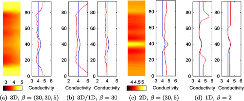
Figure 6. The cross-sections of the 3D reconstructions (Case 1) and vertical conductivity profiles (mean of the 3D conductivity (2121 $$\begin{array}{c}\hfill \mathit{\sigma }(z)=\frac{1}{R-r_0}{\int }_{r_0}^R\mathit{\sigma }(r,z)dr={\tilde{P}}_{1D}{P}_{2D}\overline{\mathit{\sigma }}=P_{1D}\overline{\mathit{\sigma }},\end{array}$$21 )). $\mathit{\beta }$ refers to the correlation length ($\mathit{\beta }=({\mathit{\beta }}_x,{\mathit{\beta }}_y,{\mathit{\beta }}_z)$) in the prior model (2929 $$\begin{array}{c}\hfill {\mathrm{\Gamma }}_{\mathrm{p}}r(i,j)=\left\{\begin{array}{cc}\hfill aexp\left\{-,\sum _{k=1}^{\mathrm{d}im},\frac{{\left(x_k^i,-,x_k^j\right)}^2}{2{\mathit{\beta }}_k^2}\right\}+{\mathit{\mu }}_{\mathrm{hg}}^2& ,\forall x_k^i,x_k^j\in {\mathrm{\Omega }}_1,\hfill \\ \hfill {\mathit{\mu }}_{\mathrm{hg}}^2& ,\forall x_k^i,x_k^j\in {\mathrm{\Omega }}_2,\hfill \\ \hfill aexp\left\{-,\sum _{k=1}^{\mathrm{d}im},\frac{{\left(x_k^i,-,x_k^l\right)}^2}{2{\mathit{\beta }}_k^2}\right\}+{\mathit{\mu }}_{\mathrm{hg}}^2& ,\forall x_k^i\in {\mathrm{\Omega }}_1,x_k^j\in {\mathrm{\Omega }}_2.\hfill \end{array}\right.\end{array}$$29 ) and ${\mathrm{\Delta }}_{\mathit{\sigma }}$ (%) are the relative reconstruction errors (3333 $$\begin{array}{c}\hfill {\mathrm{\Delta }}_{\mathit{\sigma }}=\frac{\mid \mid P_{1}D{\mathit{\sigma }}_{\mathrm{t}}rue-P_i{\mathit{\sigma }}_{\mathrm{M}AP}\mid \mid }{\mid \mid P_{1}D{\mathit{\sigma }}_{\mathrm{t}}rue\mid \mid }\times 100\%,\end{array}$$33 ).

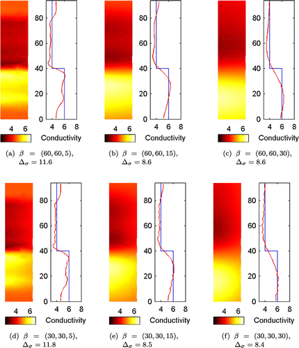
Table 2. Average computation times (s) for inverse problem using 1D, 2D, 3D-models and 3D/1D approach in Case 1.

	1D	2D	3D	3D/1D
Computation time	7	180	400	356

Figure 7. The estimated vertical conductivity profiles (Case 1) (3D/1D reconstructions). $\mathit{\beta }$ refers to correlation length ($\mathit{\beta }={\mathit{\beta }}_z$) in the prior model. On the right hand side estimates the conductivity is modelled to be homogeneous at the top and bottom end of the computation domain. ${\mathrm{\Delta }}_{\mathit{\sigma }}$ (%) are the relative reconstruction errors (3333 $$\begin{array}{c}\hfill {\mathrm{\Delta }}_{\mathit{\sigma }}=\frac{\mid \mid P_{1}D{\mathit{\sigma }}_{\mathrm{t}}rue-P_i{\mathit{\sigma }}_{\mathrm{M}AP}\mid \mid }{\mid \mid P_{1}D{\mathit{\sigma }}_{\mathrm{t}}rue\mid \mid }\times 100\%,\end{array}$$33 ). The first relative reconstruction errors are for the left figures and the second ones are for the right figures.

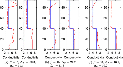
Figure 8. The 2D reconstructions (Case 1) and vertical conductivity profiles (mean of the 2D conductivity). $\mathit{\beta }$ refers to correlation length ($\mathit{\beta }=({\mathit{\beta }}_r,{\mathit{\beta }}_z)$) in the prior model and ${\mathrm{\Delta }}_{\mathit{\sigma }}$ (%) are the relative reconstruction errors (3333 $$\begin{array}{c}\hfill {\mathrm{\Delta }}_{\mathit{\sigma }}=\frac{\mid \mid P_{1}D{\mathit{\sigma }}_{\mathrm{t}}rue-P_i{\mathit{\sigma }}_{\mathrm{M}AP}\mid \mid }{\mid \mid P_{1}D{\mathit{\sigma }}_{\mathrm{t}}rue\mid \mid }\times 100\%,\end{array}$$33 ).

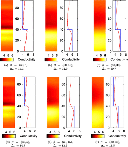
Figure 9. The 1D reconstructions (Case 1) with the approximation error approach are shown on the top row and 1D MAP-CEM reconstructions (without approximation error approach) on the bottom row. $\mathit{\beta }$ refers to the correlation length ($\mathit{\beta }={\mathit{\beta }}_z$) in the prior model. On the right hand side estimates the conductivity is modelled to be homogeneous at the ends of the computation domain. ${\mathrm{\Delta }}_{\mathit{\sigma }}$ (%) are the relative reconstruction errors (3333 $$\begin{array}{c}\hfill {\mathrm{\Delta }}_{\mathit{\sigma }}=\frac{\mid \mid P_{1}D{\mathit{\sigma }}_{\mathrm{t}}rue-P_i{\mathit{\sigma }}_{\mathrm{M}AP}\mid \mid }{\mid \mid P_{1}D{\mathit{\sigma }}_{\mathrm{t}}rue\mid \mid }\times 100\%,\end{array}$$33 ). The first relative reconstruction errors are for the left figures and the second ones are for the right figures.

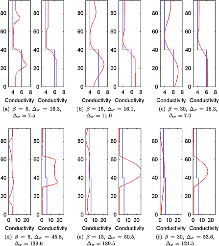
Figure 10. The estimated conductivities (Case 2). (a) 3D reconstructions (b) 3D/1D reconstruction (c) 2D reconstruction (d) 1D reconstruction.

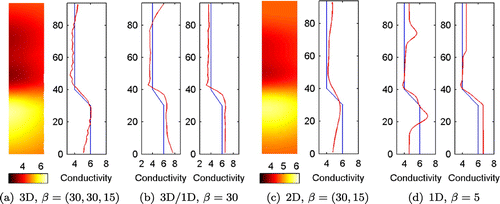
Figure 11. The sensitivity of the measurements in logarithmic scale (sum of absolute values of all rows in Jacobian matrix) with two different current patterns. (a) The adjacent current and measurement patterns that were used in the simulations. (b) The opposite current pattern and adjacent measurement pattern were used. The opposite current pattern was used in one test case, see Figure 12.

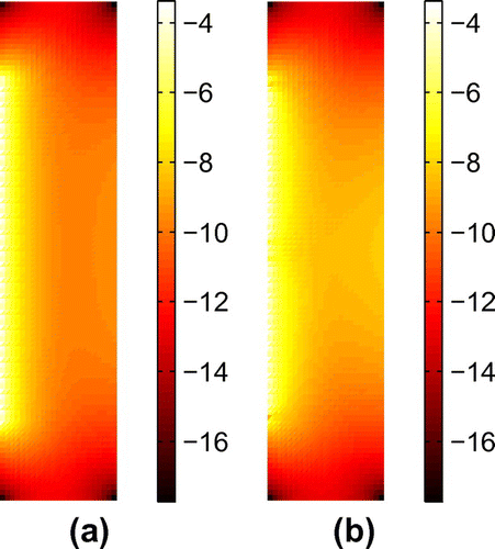
Figure 12. Estimated conductivity using 2D model with opposite current patterns. The correlation length was $\mathit{\beta }=(30,15)$.

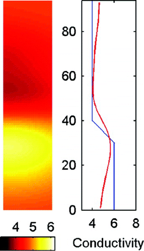
Figure 13. Estimated conductivities (Case 3). (a) 3D reconstruction (b) 3D/1D reconstruction (c) 2D reconstruction (d) 1D reconstruction.

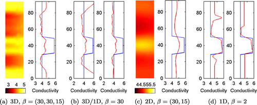
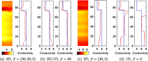
Figure 14. Estimated conductivities (Case 4). (a) 3D reconstruction (b) 3D/1D reconstruction (c) 2D reconstruction (d) 1D reconstruction (length of the homogeneous regions is 30 cm).

Figure 15. 1D reconstruction (Case 4), correlation length $\mathit{\beta }=2$. Length of the homogeneous regions is 15 cm.

Figure 16. The estimated conductivities (Case 5). (a) 3D reconstruction (b) 3D/1D reconstruction (c) 2D reconstruction (d) 1D reconstruction.

4.4 The statistics of the modelling error

The modelling error statistics was computed as explained in Section 3.4.4. The average percentual modelling error level is shown in Figure 5. As can be seen, the modelling error due to 1D forward model is very high compared to that of 2D cylindrically symmetric model. The error is particularly high on the electrodes that are near the ends of the measurement probe. This is due to the fact that the 1D model prevents the flow of currents to the electrode-free regions at the ends of the probe. The simulated conductivity samples were cylindrically symmetric and therefore the assumptions in the cylindrically symmetric model were fulfilled. The errors between 3D and cylindrically symmetric 2D model are due to discretization and different basis functions for the conductivity.

4.5 Reconstructions for Case 1

The cross-sections of the 3D reconstructions in Case 1 are shown in Figure 6 (left figures). The mean vertical conductivity profiles are shown in Figure 6 (right). The mean vertical conductivity profile was computed as $P_{1}D{\mathit{\sigma }}_{\mathrm{M}}AP$ for the estimated conductivity (red line) and for the true conductivity as $P_{1}D{\mathit{\sigma }}_{\mathrm{t}}rue$ (blue line), where $P_{1}D$ is linear mapping in (2121 $$\begin{array}{c}\hfill \mathit{\sigma }(z)=\frac{1}{R-r_0}{\int }_{r_0}^R\mathit{\sigma }(r,z)dr={\tilde{P}}_{1D}{P}_{2D}\overline{\mathit{\sigma }}=P_{1D}\overline{\mathit{\sigma }},\end{array}$$21 ). The relative reconstruction error (3333 $$\begin{array}{c}\hfill {\mathrm{\Delta }}_{\mathit{\sigma }}=\frac{\mid \mid P_{1}D{\mathit{\sigma }}_{\mathrm{t}}rue-P_i{\mathit{\sigma }}_{\mathrm{M}AP}\mid \mid }{\mid \mid P_{1}D{\mathit{\sigma }}_{\mathrm{t}}rue\mid \mid }\times 100\%,\end{array}$$33 ) is small when the correlation length is large in the direction of the $z$-axis, see Figure 6(c) and (f). These reconstructions are very smooth and the possible location of the phase interface can be said to be in the interval $z\in [20,50]$. Therefore, the relative reconstruction error (3333 $$\begin{array}{c}\hfill {\mathrm{\Delta }}_{\mathit{\sigma }}=\frac{\mid \mid P_{1}D{\mathit{\sigma }}_{\mathrm{t}}rue-P_i{\mathit{\sigma }}_{\mathrm{M}AP}\mid \mid }{\mid \mid P_{1}D{\mathit{\sigma }}_{\mathrm{t}}rue\mid \mid }\times 100\%,\end{array}$$33 ) gives misleading information about the ability to detect the location of the phase interface. To detect the location of the phase interface, the best estimates are obtained when the correlation length is small in the direction of the $z$-axis and fairly large in the direction of the $x$- and $y$-axis (Figure 6(a) and (d)). Based on these estimates, it can be said that the phase interface is in the interval $z\in [35,45]$. The conductivity estimates in the electrode-free regions at top and bottom of the computation domain are very unreliable. The vertical conductivity profiles also show the reconstruction errors in both ends of the computation domain clearly. The measurements give very small amount of information from these regions.

In Figure 7, the 3D/1D reconstructions are shown. On the left hand side figures, the reconstruction errors can be seen near the both ends of the probe similarly as in Figure 6. On right hand side figures, the conductivity is modelled to be homogeneous in the electrode-free regions $z\in [0,15]$ and $z\in [89,94]$, see Section 3.5. Clearly the reconstructions with the homogeneous model are better than those without the homogeneous model.

The 2D reconstructions are shown in Figure 8 (left figures). The mean vertical conductivity profiles are shown in Figure 8 (right). The mean vertical conductivity profile was computed as $P_{2}D{\mathit{\sigma }}_{\mathrm{M}}AP$ for the estimated conductivity (red line), and for the true conductivity as $P_{1}D{\mathit{\sigma }}_{\mathrm{t}}rue$ (blue line), where $P_{2}D$ and $P_{1}D$ are linear mappings in (2020 $$\begin{array}{c}\hfill \mathit{\sigma }(r,z)=\frac{1}{2\mathit{\pi }r}{\int }_0^{2\mathit{\pi }}\overline{\mathit{\sigma }}(r,\mathit{\theta },z)rd\mathit{\theta }=\frac{1}{2\mathit{\pi }}{\int }_0^{2\mathit{\pi }}\overline{\mathit{\sigma }}(r,\mathit{\theta },z)d\mathit{\theta }=P_{2D}\overline{\mathit{\sigma }},\end{array}$$20 ) and (2121 $$\begin{array}{c}\hfill \mathit{\sigma }(z)=\frac{1}{R-r_0}{\int }_{r_0}^R\mathit{\sigma }(r,z)dr={\tilde{P}}_{1D}{P}_{2D}\overline{\mathit{\sigma }}=P_{1D}\overline{\mathit{\sigma }},\end{array}$$21 ), respectively. As in the 3D case, the best reconstructions are obtained using large correlation length in the direction of the $r$-axis ($x$-axis in 3D) and small correlation length in the vertical direction.

The 1D reconstructions are shown in Figure 9 in the first row. The 1D MAP-CEM reconstructions (reconstructions without the approximation error approach) are shown in the second row. As can be seen, the 1D MAP-CEM reconstructions are completely useless. The reconstructions with the approximation error approach can locate the phase interface correctly. The estimated conductivity is nearest to correct values in the mid-section of the computation domain. On the right hand side figures, the conductivity is modelled to be homogeneous at the vertical locations $z\in [0,30]$ and $z\in [64,94]$. In 3D/1D reconstructions shown in Figure 7, only 15 cm intervals were used. The longer homogeneous intervals are used because the approximation errors are largest near the ends of the probe. Therefore, several measurements from the homogeneous region are needed to estimate the conductivity correctly.

The average computation times are shown in Table 2. The computation times with 1D and 2D cylindrically symmetric forward models are significantly shorter than those with conventional 3D models. The reduction in computation time by using the reduced forward models is achieved without compromising the accuracy of the reconstruction.

4.6 Reconstructions for Case 2

In the remaining cases, only the best reconstructions (chosen by visual inspection) are shown. The main criterion for the best reconstructions is the ability to locate the phase interface correctly and therefore the computed errors ${\mathrm{\Delta }}_{\mathit{\sigma }}$ were not considered. The reconstructions in Case 2 are shown in Figure 10. The location of the phase interface $(z=40)$ near the measurement probe is well estimated in all reconstructions. However, the true shape of the profile is not found that accurately further away from the probe in 2D and 3D reconstructions.

The probe measurements are most sensitive to conductivity changes near the probe, see the sensitivity of the measurements (sum of rows of the absolute values of the Jacobian matrix) in Figure 11 for adjacent and opposite current patterns. The adjacent current pattern refers here to the current pattern that is used in the simulation of the measurements and opposite patterns contain injections between the electrode pairs ((1 22) (2 21) $\dots$ (11 12)). Since the sensitivity is better with the opposite current injection, we estimated the conductivity also with this current pattern, see Figure 12. As can be seen, the reconstruction is only slightly better than that with the adjacent injection.

4.7 Reconstructions for Case 3

The reconstructions in the Case 3 are shown in Figure 13. All of the reconstructions capture the location of the inclusion to some extend. The estimated value near the inclusion are closest to the true values using the 1D model. It was also found that the best reconstructions were produced with very different correlation lengths. The correlation length was 30 cm in 3D/1D reconstruction and 2 cm in 1D reconstruction.

4.8 Reconstructions for Case 4

The reconstructions in the Case 4 are shown in Figure 14. The location of the phase interface is found using all models. This case is difficult for the 1D model since the phase interface is near the top region of the measurement probe and as discussed earlier the modelling errors are largest on the measurements near the ends of the probe. As can be seen in Figure 14(d) (right), the reconstruction does not give reliable results when too long (30 cm) homogeneous region is modelled to the ends of the computation domain. In Figure 15, the length of the homogeneous regions is decreased to 15 cm. With this prior model, the reconstructed conductivity profile is more accurate than that with the longer homogeneous regions although there are still some reconstruction errors on both sides of the interface.

4.9 Reconstructions for Case 5

The reconstruction in the Case 5 is shown in Figure 16. The true conductivity (sphere-shaped inclusion in homogeneous background) violates the symmetry assumptions of the conductivity in the reduced forward models. Therefore, this test case can be considered as a difficult case. The reconstructions with the cylindrically symmetric and 1D forward model reconstruct the inclusion more accurately than the 3D model.

5 Conclusions

In this paper, two reduced forward models for EIT in probe geometry were proposed. The aim was to reduce the computation time and take into account certain symmetry of the conductivity. In phase interface detection applications, the conductivity can often be assumed to be rotationally invariant. In this case, it is tempting to use the 2D forward model which is computationally more efficient than a full 3D model. However, the conventional 2D forward model is very approximative and causes reconstruction errors when static EIT imaging is employed. In this study, the 2D cylindrically symmetric forward model which takes into account the rotational invariance of the conductivity was proposed. As a second model, 1D forward model was proposed to further decrease the computation time. The 1D forward model is highly approximative and the reconstructions with this model using the conventional error model are useless. The Bayesian approximation error approach was applied to compensate the modelling errors. In the approximation error approach, the statistics of the modelling error is estimated and used in the inverse problem. By using approximation error approach, feasible reconstructions with the approximative forward models can be efficiently computed.

Five simulated examples of phase interface detection were considered. The location of the phase interface is an important parameter in flotation and sedimentation processes, for example. The 3D reconstructions were computed as reference estimates. It was found that the reconstructions using reduced forward models produced useful estimates in all cases. The conventional 3D reconstructions are more robust than those with 1D forward model when the phase interface is near the upper or lower end of the electrode array. This is due to the fact that the level of the modelling error is highest near the ends of the measurement probe. In one test case, feasible econstructions with reduced forward models were computed when the actual conductivity was not cylindrically symmetric. The variance of the inhomogeneous part had to be chosen very large in the prior model when the 1D model was used. The results with smaller variances in the prior model were worse using both the conventional and approximation error model. Based on the results, the reconstructions with the 1D model should be tested with wide range of the prior parameters. The computation times with the reduced forward models are significantly shorter compared to approaches with 3D models. The reduction of the computation time is achieved without compromising the ability to estimate the location of the phase interface. The computation time with 1D forward model was approximately 1/50 of that with 3D forward model. The reconstruction time is limited in most of the industrial applications since the process control is done in real time. Therefore, the reduced forward models can be useful when static images have to be computed in limited time.

The proposed approach can be applied to other applications with probe geometry as well as to other measurement geometries. For example, the translational invariance of the conductivity could be taken into account by using this approach. Two-dimensional forward models are typically used when one layer of electrodes is attached around the measurement target. One layer of electrodes is used in biomedical applications when the electrodes are typically attached around the patients chest and in industrial pipe flow measurements, the electrodes are attached around the flow pipe. In these cases, the reconstruction accuracy and speed could be improved by modelling the invariance of the conductivity in the direction of the central axis of the target.

Acknowledgments

The work was supported by the TEKES projects 2172/31/2010 and 2180/31/2011. Furthermore, this work was supported by the Academy of Finland (project 250215 Finnish Centre of Excellence in Inverse Problems Research). D. Sbarbaro also acknowledges the partial support of Fondecyt Project 1100272.

References

- Cheney M, Isaacson D, Newell JC. Electrical impedance tomography. SIAM Rev. 1999;41:85–101.
- Kaipio JP, Kolehmainen V, Somersalo E, Vauhkonen M. Statistical inversion and Monte Carlo sampling methods in electrical impedance tomography. Inv. Probl. 2000;16:1487–1522.
- Borcea L. Electrical impedance tomography. Inv. Probl. 2002;18:R99–R136.
- Brown BH. Electrical impedance tomography (EIT): a review. J. Med. Eng. Technol. 2003;27:97–108.
- Bayford R. Bioimpedance tomography (electrical impedance tomography). Annu. Rev. Biomed. Eng. 2006;8:63–91.
- Lehikoinen A, Laakkonen P, Vauhkonen M, Rinne A, Saloheimo K, Lähteenmäki S. Measuring flotation process using probe sensor based on 3D electrical resistance tomography. In: Flotation’11; 2011; Cape Town.
- Vauhkonen M, Lehikoinen A, Kourunen J, Mononen M, Huuskonen J. Flotation process optimization using Outotec Froth Control solution. In: Canadian Mineral Processors 2013; 2013; Ottawa.
- Ider YZ, Gencer NG, Atalar E, Tosun H. Electrical impedance tomography of translationally uniform cylindrical objects with general cross-sectional boundaries. IEEE Trans. Med. Imaging. 1990;9:49–59.
- Jerbi K, Lionheart WRB, Vauhkonen PJ, Vauhkonen M. Sensitivity matrix and reconstruction algorithm for EIT assuming axial uniformity. Physiol. Meas. 2000;21:61–66.
- Ammari H, Garnier J, Solna K. Resolution and stability analysis in full-aperture, linearized conductivity and wave imaging. Proc. Am. Math. Soc. 2013;141:3431–3446.
- Ammari H, Garnier J, Solna K. Partial data resolving power of conductivity imaging from boundary measurements. SIAM J. Math. Anal. 2013;45:1704–1722.
- Ammari H, Deng Y, Kang H, Lee H. Reconstruction of inhomogeneous conductivities via the concept of generalized polarization tensors. Annales de l’Institut Henri Poincare (C) Non Linear, Analysis. in press.
- Kaipio JP, Somersalo E. Statistical and computational inverse problems. Vol. 160, Applied Mathematical Sciences. New York (NY): Springer-Verlag; 2005.
- Kaipio JP, Somersalo E. Statistical inverse problems: discretization, model reduction and inverse crimes. J. Comput. Appl. Math. 2007;198:493–504.
- Nissinen A, Heikkinen LM, Kaipio JP. The Bayesian approximation error approach for electrical impedance tomography–experimental results. Meas. Sci. Technol. 2008;19:015501.
- Lehikoinen A, Finsterle S, Voutilainen A, Heikkinen LM, Vauhkonen M, Kaipio JP. Approximation errors and truncation of computational domains with application to geophysical tomography. Inv. Probl. Imaging. 2007;1:371–389.
- Nissinen A, Heikkinen LM, Kolehmainen V, Kaipio JP. Compensation of errors due to discretization, domain truncation and unknown contact impedances in electrical impedance tomography. Meas. Sci. Technol. 2009;20:105504.
- Nissinen A, Kolehmainen V, Kaipio JP. Compensation of modelling errors due to unknown domain boundary in electrical impedance tomography. IEEE Trans. Med. Imaging. 2011;30:231–242.
- Nissinen A, Kolehmainen V, Kaipio JP. Reconstruction of domain boundary and conductivity in electrical impedance tomography using the approximation error approach. I. J. Uncertainty Quantification. 2011;1:203–222.
- Heino J, Somersalo E. A modeling error approach for the estimation of optical absorption in the presence of anisotropies. Phys. Med. Biol. 2004;49:4785–4798.
- Heino J, Somersalo E, Kaipio JP. Compensation for geometric mismodelling by anisotropies in optical tomography. Opt. Express. 2005;13:296–308.
- Arridge SR, Kaipio JP, Kolehmainen V, Schweiger M, Somersalo E, Tarvainen T, Vauhkonen M. Approximation errors and model reduction with an application in optical diffusion tomography. Inv. Probl. 2006;22:175–195.
- Kolehmainen V, Schweiger M, Nissilä I, Tarvainen T, Arridge SR, Kaipio JP. Approximation errors and model reduction in three-dimensional diffuse optical tomography. J. Opt. Soc. Am. 2009;26:2257–2268.
- Tarvainen T, Kolehmainen V, Pulkkinen A, Vauhkonen M, Schweiger M, Arridge SR, Kaipio JP. Approximation error approach for compensating modelling errors between the radiative transfer equation and the diffusion approximation in diffuse optical tomography. Inv. Probl. 2010;26:015005 (18pp).
- Kolehmainen V, Tarvainen T, Arridge SR, Kaipio JP. Marginalization of uninteresting distributed parameters in inverse problems – application to diffuse optical tomography. Int. J. Uncertainty Quantification. 2011;1:1–17.
- Cheng KS, Isaacson D, Newell JC, Gisser DG. Electrode models for electric current computed tomography. IEEE Trans. Biomed. Eng. 1989;36:918–924.
- Somersalo E, Cheney M, Isaacson D. Existence and uniqueness for electrode models for electric current computed tomography. SIAM J. Appl. Math. 1992;52:1023–1040.
- Vauhkonen PJ, Vauhkonen M, Savolainen T, Kaipio JP. Three-dimensional electrical impedance tomography based on the complete electrode model. IEEE Trans. Biomed. Eng. 1999;46:1150–1160.
- Tarantola A. Inverse problem theory and methods for model parameter estimation. Philadelphia (PA): SIAM; 2004.
- Calvetti D, Somersalo E. An introduction to Bayesian scientific computing –- ten lectures on subjective computing. New York (NY): Springer; 2007.
- Lieberman C, Willcox K, Ghattas O. Parameter and state model reduction for large-scale statistical inverse problems. SIAM J. Sci. Comput. 2010;32:2523–2542.