Approaches to accommodate noisy data in the direct solution of inverse problems in incompressible plane strain elasticity

Abstract

We apply the adjoint-weighted equation method (AWE) to the direct solution of inverse problems of incompressible plane strain elasticity. We show that based on untreated noisy displacements, the reconstruction of the shear modulus can be very poor. We link this poor performance to loss of coercivity of the weak form when treating problems with discontinuous coefficients. We demonstrate that by smoothing the displacements and appending a regularization term to the AWE formulation, a dramatic improvement in the reconstruction can be achieved. With these improvements, the advantages of the AWE method as a direct solution approach can be extended to a wider range of problems.

Keywords:

• variational methods
• inverse problems
• incompressible plane strain
• smoothing
• regularization

1 Introduction

It has long been recognized that changes in tissue stiffness can indicate pathological developments. Manual palpation, which involves applying compression to various parts of the body in order to detect abnormalities, is routinely practised by physicians as a first line of diagnosis. While manual palpation can provide a quick qualitative assessment of the patient’s conditions, it suffers many limitations: it is highly dependent on the physician’s skill and experience, it is limited to pathological changes that are significant enough to be felt and can not provide a quantitative measure of the actual tissue structure.

The term ‘elastography’ was coined by Ophir and colleagues to refer to the imaging and assessment of pathological changes associated with changes in tissue stiffness.[1–9] When first proposed, the aim of elastography was to provide strain images of tissues under load, and from these strains infer the mechanical properties. The main idea was that when subjected to mechanical load, soft tissue deforms more than stiff tissue, and therefore tissue stiffness can be related to the reciprocal of the strain. While this method can provide a qualitative picture of the tissue stiffness, it is valid only for some very simple cases. In most cases of general loadings and inhomogeneous materials, the reciprocal of the strain is not directly proportional to actual tissue stiffness, and assuming so could lead to incorrect reconstruction of tissue properties. In certain cases, quantitative values of the mechanical properties are considered useful for identification of pathologies (e.g. differentiate benign from malignant lesions [10]). For this purpose, qualitative indications such as displacement or strain imaging are inadequate.

In order to obtain a more accurate estimate of the elastic properties of a tissue, an inverse elasticity problem must be solved. The main approach to solving inverse problems of elasticity is through iterative optimization.[11–13] This approach is robust and allows reconstruction of tissue properties from the measured displacement fields even in cases where these are only partially available or are corrupted by noise. On the other hand, the iterative procedure can involve long computational times, on the order of a few minutes. In real-time ultrasound imaging applications, this wait time is thought to be prohibitive. In cases where full-field displacement data are available on the other hand, a direct solution approach can be employed.[14–17] Here, the solution can be obtained in a single solve without the need to iterate.

The adjoint-weighted equation (AWE) method is a novel variational formulation for direct solution of inverse problems. The AWE method was first proposed for problems of thermal conductivity,[14] and was later extended to general problems of elasticity.[15–17] The AWE variational formulation has desirable properties. With sufficiently smooth data, it leads to a provably well-posed linear variational problem for the modulus distribution. A straightforward Galerkin discretization leads to a stable and optimally convergent numerical method, even for data corrupted with error.

The stability of the AWE formulation, however, depends on the continuity of the data.[15] As shown in [15], when the data involve discontinuities, coercivity, and hence numerical stability, is lost and the performance of the AWE method may be compromised.

There are two main sources for discontinuities in the data. The first is that the target itself may have a discontinuous distribution of properties, such as presented by a homogeneous inclusion in an otherwise homogeneous background of different properties. In this case, the strain formally has infinite gradients at the discontinuity. Secondly, the presence of random noise in the measurement can lead to large gradients of strain, which also can lead to a loss of coercivity of the AWE weak form.

Therefore, the presence of random noise in the data can have a deleterious impact in several ways. Most obviously, of course, noise leads to a loss of accuracy introduced by inaccuracy in the data. Secondly, the non-linear dependence of the AWE variational formulation on the data leads to a non-linear dependence on the noise amplitude. Finally, and of most concern in the present study, is the potential loss of stability of the formulation with rough random noise. That is, the presence of noise not only leads to inaccuracies in the solution, but alters the basic mathematical properties of the variational formulation of the inverse problem.

In this study, we concern ourselves with practical approaches to mitigate the deleterious impact of noise on the results of the AWE variational formulation. Our focus is on managing the loss of numerical stability associated with discontinuous and/or noisy data. To that end, we consider two approaches to address this problem. One is smoothing the data to lessen the impact of sharp gradients. The second is stabilizing the formulation by adding a regularization term. We apply these approaches to several problems, including both synthetic and experimental data. We find that using these approaches yields a dramatic improvement in the performance of the AWE method.

2 Formulation

2.1 Inverse problem of isotropic incompressible plane strain elasticity

Consider the equilibrium equations of elasticity in the absence of body forces:1 $$\begin{array}{c}\hfill \nabla ·\mathit{\sigma }=0\end{array}$$1 Here $\mathit{\sigma }$ is the Cauchy stress tensor, which, for an incompressible isotropic linear elastic material takes the form:2 $$\begin{array}{c}\hfill {\mathit{\sigma }}_{ij}=-p{\mathit{\delta }}_{ij}+2\mathit{\mu }{\mathit{ϵ}}_{ij}\end{array}$$2 Here $p$ represents the pressure, $\mathit{\mu }$ is the shear modulus and $\mathit{ϵ}$ is the strain tensor (the symmetric part of the displacement gradient). With this definition, the equilibrium equation becomes:3 $$\begin{array}{c}\hfill -\nabla p+2\nabla ·(\mathit{\mu }\mathit{ϵ})=\mathbf{0}\end{array}$$3 The standard problem of incompressible elasticity for displacements is subject to the constraint of preservation of volume, namely $\text{tr}(\mathit{ϵ})=0$. Consider the following inverse problem of isotropic incompressible plane strain elasticity: Given a strain field $\mathit{ϵ}$ in $\mathrm{\Omega }\subset {\mathbb{R}}^2$, find $\mathit{\mu }(\mathbf{x})$ and $p(\mathbf{x})$ satisfying Equation (33 $$\begin{array}{c}\hfill -\nabla p+2\nabla ·(\mathit{\mu }\mathit{ϵ})=\mathbf{0}\end{array}$$3 ). Here, in contrast to the standard (‘forward’) elasticity problem, the strains $\mathit{ϵ}$ are given data arising from measured displacements. Note that compared to the forward problem of elasticity, which is governed by a second-order elliptic partial differential equation for the displacements, the inverse problem is governed by a first-order system equation for the shear modulus and pressure.

The solution to partial differential equations without boundary data involves arbitrary functions. This is also the case for the inverse problem of incompressible plane strain with a single deformation field available, since boundary data (i.e. the shear modulus and pressure fields) are usually unknown a-priori. A solution in terms of arbitrary functions is too general for practical modulus reconstruction purposes. One way to cope with this challenge is to use an additional deformation field taken from the same elastic body, but with different loadings applied. This provides additional equations without increasing the unknown number of shear modulus distributions (since it is the same elastic body). Properties of the inverse problem of isotropic incompressible plane strain elasticity with two strain fields were considered in [18]. It is shown that the most general solution no longer involves arbitrary functions, but instead involves up to four arbitrary constants for the shear modulus. One additional arbitrary constant is also attributed to each of the two pressure fields. To remove the arbitrariness associated with the four constants related to the shear modulus, it is sufficient to know its value at four distinct points. For biomedical imaging applications, these can often be measured, for example along the exposed skin surface. Finally, since in the context of shear modulus reconstruction the pressure fields are often of no interest, their value at a point can be prescribed arbitrarily.

Consider a sub-region in the domain, $\overline{\mathrm{\Omega }}\subset \mathrm{\Omega }$, where the shear modulus distribution $\overline{\mathit{\mu }}$ is available. We refer to this region as a ‘calibration region’ and use it to impose the known shear modulus distribution via a single continuous calibration condition of the form:4 $$\begin{array}{c}\hfill \mathit{\mu }=\overline{\mathit{\mu }}\text{in}\overline{\mathrm{\Omega }}.\end{array}$$4 Satisfaction of this condition in the $L_2$ least-squares sense is enforced by the penalty method.

2.2 AWE variational method

The AWE method was first proposed for the solution of inverse thermal problems where the conductivity is the unknown.[14] The method is based on a variational formulation that is weighted by the adjoint operator, suggested by adjoint-stabilized finite element methods [19] that arise in the variational multiscale framework.[20] It is motivated by the goal to find optimal approximate solutions for partial differential equations presented in [21], and may be seen as a formal limit of the streamline upwind Petrov-Galerkin method,[22, 23] as the stabilization parameter becomes unbounded.

In what follows, we consider the AWE method for incompressible plane strain elasticity. We set up the equations based on the generalized formulation,[16] and employ two data-sets of strains.

Consider the AWE formulation for incompressible plane strain, with two strain fields provided. We seek functions $\mathit{\mu },p_1,p_2\in H^1(\mathrm{\Omega })$ such that $\forall w_1,w_2,w_3\in H^1(\mathrm{\Omega })$:5 $$\begin{array}{c}\hfill (2{\mathit{ϵ}}_1\nabla w_1,\nabla ·(2{\mathit{ϵ}}_1\mathit{\mu }-\mathbf{1}{p}_1))+(2{\mathit{ϵ}}_2\nabla w_1,\nabla ·(2{\mathit{ϵ}}_2\mathit{\mu }-\mathbf{1}{p}_2))=0\end{array}$$5 6 $$\begin{array}{c}\hfill (-\nabla w_2,\nabla ·(2{\mathit{ϵ}}_1\mathit{\mu }-\mathbf{1}{p}_1))=0\end{array}$$6 7 $$\begin{array}{c}\hfill (-\nabla w_3,\nabla ·(2{\mathit{ϵ}}_2\mathit{\mu }-\mathbf{1}{p}_2))=0\end{array}$$7 Here ${\mathit{ϵ}}_1$ and ${\mathit{ϵ}}_2$ are two strain fields with distinct principal directions, $p_1$ and $p_2$ are the unknown hydrostatic pressures associated with each of the strain fields, respectively, and $\mathit{\mu }$ is the sought shear modulus. Equations (55 $$\begin{array}{c}\hfill (2{\mathit{ϵ}}_1\nabla w_1,\nabla ·(2{\mathit{ϵ}}_1\mathit{\mu }-\mathbf{1}{p}_1))+(2{\mathit{ϵ}}_2\nabla w_1,\nabla ·(2{\mathit{ϵ}}_2\mathit{\mu }-\mathbf{1}{p}_2))=0\end{array}$$5 )–(77 $$\begin{array}{c}\hfill (-\nabla w_3,\nabla ·(2{\mathit{ϵ}}_2\mathit{\mu }-\mathbf{1}{p}_2))=0\end{array}$$7 ) provide a system of three equations for the three unknown fields ($\mathit{\mu },p_1,p_2$). The calibration condition on the shear modulus is enforced by a penalty term appended to Equation (55 $$\begin{array}{c}\hfill (2{\mathit{ϵ}}_1\nabla w_1,\nabla ·(2{\mathit{ϵ}}_1\mathit{\mu }-\mathbf{1}{p}_1))+(2{\mathit{ϵ}}_2\nabla w_1,\nabla ·(2{\mathit{ϵ}}_2\mathit{\mu }-\mathbf{1}{p}_2))=0\end{array}$$5 ), leading to8 $$\begin{array}{c}\hfill \left(2,{\mathit{ϵ}}_1,\nabla ,w_1,,,\nabla ,·,\left(2,{\mathit{ϵ}}_1,\mathit{\mu },-,\mathbf{1},p_1\right)\right)+\left(2,{\mathit{ϵ}}_2,\nabla ,w_1,,,\nabla ,·,\left(2,{\mathit{ϵ}}_2,\mathit{\mu },-,\mathbf{1},p_2\right)\right)+k{\left(w_1,,,\mathit{\mu },-,\overline{\mathit{\mu }}\right)}_{\overline{\mathrm{\Omega }}}=0\end{array}$$8 In Equation (88 $$\begin{array}{c}\hfill \left(2,{\mathit{ϵ}}_1,\nabla ,w_1,,,\nabla ,·,\left(2,{\mathit{ϵ}}_1,\mathit{\mu },-,\mathbf{1},p_1\right)\right)+\left(2,{\mathit{ϵ}}_2,\nabla ,w_1,,,\nabla ,·,\left(2,{\mathit{ϵ}}_2,\mathit{\mu },-,\mathbf{1},p_2\right)\right)+k{\left(w_1,,,\mathit{\mu },-,\overline{\mathit{\mu }}\right)}_{\overline{\mathrm{\Omega }}}=0\end{array}$$8 ), $\overline{\mathrm{\Omega }}$ denotes the calibration region, within which, the shear modulus is known to be $\overline{\mathit{\mu }}$. The penalty constant is $k$.

3 Treatment of noise and non-smooth solutions

The coefficients of Equation (88 $$\begin{array}{c}\hfill \left(2,{\mathit{ϵ}}_1,\nabla ,w_1,,,\nabla ,·,\left(2,{\mathit{ϵ}}_1,\mathit{\mu },-,\mathbf{1},p_1\right)\right)+\left(2,{\mathit{ϵ}}_2,\nabla ,w_1,,,\nabla ,·,\left(2,{\mathit{ϵ}}_2,\mathit{\mu },-,\mathbf{1},p_2\right)\right)+k{\left(w_1,,,\mathit{\mu },-,\overline{\mathit{\mu }}\right)}_{\overline{\mathrm{\Omega }}}=0\end{array}$$8 ) are composed of strain data obtained by differentiation of the measured displacement field. While some imaging methods provide more accurate displacement measurements than others, all are associated with some degree of noise. When noisy displacement measurements are differentiated for the strains, the deleterious effects of the noise on the solution are amplified. When considering (88 $$\begin{array}{c}\hfill \left(2,{\mathit{ϵ}}_1,\nabla ,w_1,,,\nabla ,·,\left(2,{\mathit{ϵ}}_1,\mathit{\mu },-,\mathbf{1},p_1\right)\right)+\left(2,{\mathit{ϵ}}_2,\nabla ,w_1,,,\nabla ,·,\left(2,{\mathit{ϵ}}_2,\mathit{\mu },-,\mathbf{1},p_2\right)\right)+k{\left(w_1,,,\mathit{\mu },-,\overline{\mathit{\mu }}\right)}_{\overline{\mathrm{\Omega }}}=0\end{array}$$8 ), we observe that the measured displacements are differentiated twice – first the displacements are differentiated to provide the strains, and then the strains are differentiated in the equation. With these two differentiations, even a small amount of noise can have a significant effect on the solution. Therefore, some treatment of the problem is often necessary.

In [15], it is shown that the conditioning of the AWE system deteriorates with roughness of the coefficients. This can occur with noise in the data, but can also occur in perfect data if the shear modulus distribution itself is not continuous.

Below we present two methods to ameliorate the effects of rough strain measurements. One uses smoothed data in the original variational formulation. The second augments the original AWE variational formulation with a stabilizing regularization term.

3.1 Smoothing the strain field

One method to deal with noise is by smoothing the noisy measurements.[24] We note that since the strain components appear as coefficients in a first-order advective system, the smoothing procedures described below may be interpreted as a form of Leray regularization. This form of regularization has been used to generate large eddy simulation models for fluid turbulence.[25] There, the rough velocity field in the advective term is replaced by a smoother, filtered version. In this way, a more regular solution of the Navier-Stokes equation is obtained. In a similar way, we consider two forms of smoothing below: spatially averaging the measurements and down-sampling the measurements to a coarser grid.

3.1.1 Smoothing by spatial averaging

We first consider spatial averaging. Here, the value of the measured displacement at each measurement point is replaced with the average value of several neighbouring points on a grid containing the measured displacements. When the noise is random, averaging can reduce the noise level significantly. The amount of smoothing can be controlled by the number of points averaged; increasing the number of points increases the level of smoothing. This however comes at the expense of also smearing the solution and losing sharp edges.

3.1.2 Smoothing by down-sampling

Another method of smoothing is by down-sampling the measured displacements. When considering compatible (noise-free) displacement fields, continuity of the displacements is satisfied. In the presence of noise, however, this continuity is lost. For a given level of noise on the displacements, this loss of continuity becomes more evident when measurements are taken on fine grids (the change in the displacement value between two adjacent measurement points is more influenced by the noise). When differentiating these noisy displacements, the strains will be very different from those of the noise-free field. The down-sampling procedure involves increasing the space between the measured points by removing some of them from the grid, effectively reducing the influence of the noise. Of course, the down-sampling procedure comes at the expense of losing the information at the points removed, and ending up with a coarse grid of points. One way to improve the results is to interpolate the down-sampled displacement field back onto a finer grid. In what follows, we shall consider two interpolations: the first is that of the down-sampled displacements themselves and the second is of the strain field obtained from the differentiated down-sampled displacements.

3.2 Regularization of the AWE formulation

A second method to improve performance in the presence of noise is by adding stability to the formulation through a regularization term. This can be done instead of, or in addition to, smoothing the measured displacements. In this section, we augment the AWE formulation with a total variation (TV) regularization term [17, 26, 27] which is well suited for piecewise constant solutions. The TV regularization is useful for reducing the effect of noise while still preserving sharp gradients in the solution. Such sharp gradients appear in the inclusion problems we will consider which resemble problems encountered in biomedical imaging. The total variation regularization is approximated in the form:9 $$\begin{array}{c}\hfill R(\mathit{\mu })={\int }_{\mathrm{\Omega }}\sqrt{{\left|\nabla ,\mathit{\mu }\right|}^2+{\mathit{\beta }}^2}\end{array}$$9 We augment (55 $$\begin{array}{c}\hfill (2{\mathit{ϵ}}_1\nabla w_1,\nabla ·(2{\mathit{ϵ}}_1\mathit{\mu }-\mathbf{1}{p}_1))+(2{\mathit{ϵ}}_2\nabla w_1,\nabla ·(2{\mathit{ϵ}}_2\mathit{\mu }-\mathbf{1}{p}_2))=0\end{array}$$5 ) (the AWE equation related to the shear modulus) with $D_{\mathit{\mu }}R(\mathit{\mu })[w_1]$ to obtain:10 $$\begin{array}{cc}\hfill \left(2,{\mathit{ϵ}}_1,\nabla ,w_1,,,\nabla ,·,\left(2,{\mathit{ϵ}}_1,\mathit{\mu },-,\mathbf{1},p_1\right)\right)& +\left(2,{\mathit{ϵ}}_2,\nabla ,w_1,,,\nabla ,·,\left(2,{\mathit{ϵ}}_2,\mathit{\mu },-,\mathbf{1},p_2\right)\right)\hfill \\ \hfill & +\mathit{\alpha }\left(\nabla ,w_1,,,\frac{\nabla \mathit{\mu }}{\sqrt{{\left|\nabla ,\mathit{\mu }\right|}^2+{\mathit{\beta }}^2}}\right)=0\hfill \end{array}$$10 Here $\mathit{\alpha }$ is a parameter that controls the amount of regularization and $\mathit{\beta }$ is a constant used to assure continuity at $\left|\nabla ,\mathit{\mu }\right|=0$. The regularization term added in (1010 $$\begin{array}{cc}\hfill \left(2,{\mathit{ϵ}}_1,\nabla ,w_1,,,\nabla ,·,\left(2,{\mathit{ϵ}}_1,\mathit{\mu },-,\mathbf{1},p_1\right)\right)& +\left(2,{\mathit{ϵ}}_2,\nabla ,w_1,,,\nabla ,·,\left(2,{\mathit{ϵ}}_2,\mathit{\mu },-,\mathbf{1},p_2\right)\right)\hfill \\ \hfill & +\mathit{\alpha }\left(\nabla ,w_1,,,\frac{\nabla \mathit{\mu }}{\sqrt{{\left|\nabla ,\mathit{\mu }\right|}^2+{\mathit{\beta }}^2}}\right)=0\hfill \end{array}$$10 ) may be interpreted as a discontinuity capturing operator, similar to that used in computational fluid dynamics to treat shocks.[28–31] There are well-known procedures for selecting the parameter of Tikhonov-type regularization,[32] including unbiased predictive risk estimate, generalized cross-validation, discrepancy principle and L-curve. In the present formulation, however, the regularization is not quadratic, nor do we formulate the problem in a least-squares sense, so that these procedures would not apply directly, and others are not readily available. Instead, we propose some guidelines for selection of the regularization parameter when the noise level can be estimated, and based on some a-priori knowledge about the solution, if available. These are presented in the appendix.

The TV regularization gives rise to non-linear equations with the calibration data acting as a load. We use eight increments with each taking 3–7 Newton iterations to converge. Therefore, up to 60 solves were necessary to obtain a solution compared to a single solve without regularization. Even with this increase in computational effort, it is still well below the computational cost of most optimization procedures.

4 Computational examples

4.1 Description

In this section, we test the performance of the AWE formulation with the two approaches to regularization. We first demonstrate convergence of the method under ideal circumstances. Next we consider several inclusion problems involving synthetic data, which are motivated by problems encountered in the field of biomedical imaging. We will consider inclusions with smoothly varying material properties and inclusions involving a discontinuity in material properties (stepped inclusions). Finally, we consider an inclusion problem involving experimental data. The data are measured in a gelatin phantom using ultrasound.

4.2 Convergence study

The generalized AWE formulation leads to a convergent method provided that certain conditions on the measured strains are satisfied.[16] Consider the following two strain fields:11 $$\begin{array}{c}\hfill {\mathit{ϵ}}_1=\left[\begin{array}{cc}1& e^{-2x}+x\\ e^{-2x}+x& -1\end{array}\right]{\mathit{ϵ}}_2=\left[\begin{array}{cc}0& e^{-2y}\\ e^{-2y}& 0\end{array}\right]\end{array}$$11 A corresponding non-trivial smooth analytical shear modulus distribution satisfying the inverse problem (33 $$\begin{array}{c}\hfill -\nabla p+2\nabla ·(\mathit{\mu }\mathit{ϵ})=\mathbf{0}\end{array}$$3 ) is:12 $$\begin{array}{c}\hfill \mathit{\mu }=e^{x+y}\end{array}$$12 Two pressure distributions corresponding to the first and second strain fields are, respectively:13 $$\begin{array}{cc}\hfill p_1& =2x{e}^{x+y}-2e^{-x+y}\hfill \end{array}$$13 14 $$\begin{array}{cc}\hfill p_2& =-2e^{x-y}\hfill \end{array}$$14 The problem is solved numerically in a square domain using structured meshes of bilinear elements sequentially refined from $8\times 8$ to $256\times 256$ elements. 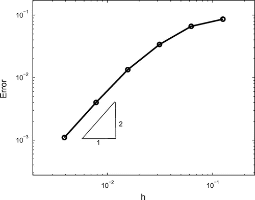The calibration region is composed of a strip of full width and $1/12$ height at the bottom of the domain where the shear modulus distribution is assumed to be known. Since the solution to the problem involves smoothly varying material properties and there is no noise in the data, smoothing and regularization are not used and the AWE solution is expected to converge to the analytical solution. Figure 1 depicts the error in the $L_2$ norm with respect to mesh refinement. Note that the slope of the curve is 2, which implies second-order convergence (in the logarithmic scale). For the bilinear finite elements used, this means that optimal rate of convergence with respect to the mesh parameter is achieved.

Figure 1. Convergence of the AWE method with mesh refinement.

4.3 Inclusion problems

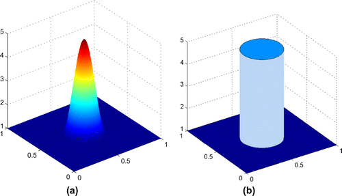
We wish to reconstruct two types of circular inclusions in a homogeneous background. The first has a smooth profile (Figure 2(a)), with the shear modulus smoothly increasing from the interface with the homogeneous background to a maximum contrast of 5:1 at the centre. The second profile is stepped (Figure  2(b)). Here, the inclusion is homogeneous, and a discontinuity exists on the interface. The contrast (between the two homogeneous regions) is 5:1. The calibration region is composed of a strip of full width and $1/12$ height at the bottom of the domain where the shear modulus distribution is assumed to be known.

Figure 2. Modulus distribution to be reconstructed: (a) circular inclusion with smoothly varying material properties and (b) a homogeneous inclusion.

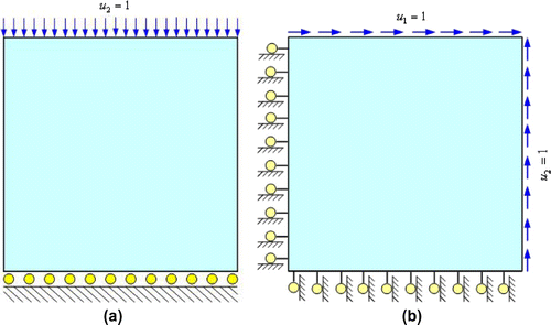
The strain fields for each inverse problem are generated synthetically by solving two forward problems, one with a compression load (Figure 3(a)) and the second with a shear load (Figure  3(b)). These provide two strain fields with distinct principal directions.

Figure 3. Loads for generating ‘synthetic data’: (a) compression test and (b) shear test.

To solve the incompressible plane strain elasticity forward problem, we use a displacement formulation with selective reduced integration.[33] The problem is solved on a mesh of $100\times 100$ bilinear elements and the displacements are then down-sampled to a $50\times 50$ mesh in order to avoid an ‘inverse crime’. To obtain a continuous strain distribution, we use an $L_2$ projection of the symmetric part of the displacement gradient.

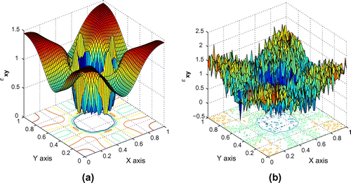
Figure 4 depicts a sample solution to the forward problem with a stepped inclusion using the shear load. Figure 4(a) presents the strain field obtained from noise-free displacements. Sharp gradients associated with the discontinuity in material properties are evident along the interface with the inclusion. Figure 4(b) presents the strain field obtained from displacements that have been corrupted by white gaussian noise, resulting in 30% noise in the strain field. This strain field is very different from the noise-free field and reconstruction of material properties using this data is expected to be challenging.

Figure 4. Strain field for the stepped inclusion problem: (a) without noise (b) and with 30% noise.

4.3.1 Reconstruction with noise-free data

We first investigate the ideal case where the strain data are derived from noise-free displacement measurements. Although actual measurements always involve a certain amount of noise, these tests can provide useful insight on the performance that can be achieved using the AWE method under optimal conditions.

Using the synthetically generated continuous strains, the inverse problem is solved on a mesh of $50\times 50$ bilinear square elements. Figure 5 presents the recovered material properties obtained for the smooth profile. The results obtained by the AWE method for this profile are very accurate. In this case, we might reasonably expect good results since the target solution is smooth and hence in $H^1$. 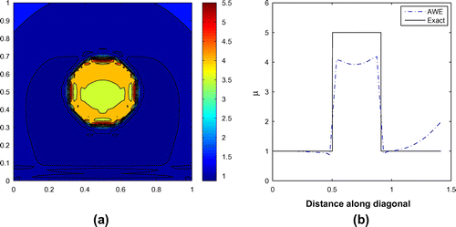Figure 6 presents the recovered material properties obtained for the stepped profile. The AWE method struggles more with this case. Though the interface between the background and the circular inclusion is sharp and well defined and the inclusion itself appears relatively homogeneous, about 20% of the targeted contrast is lost, and the background is drifting away from the correct value with distance from the calibration layer.

Figure 5. Smooth inclusion problem: (a) recovered shear modulus in the entire region and (b) along the diagonal.

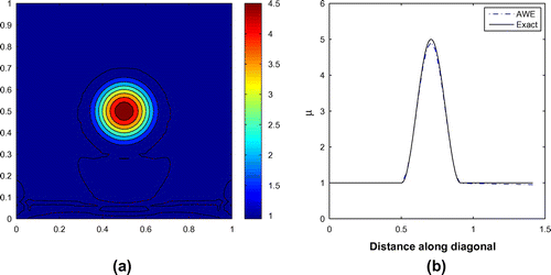
Figure 6. Stepped inclusion problem: (a) recovered shear modulus in the entire region and (b) along the diagonal.

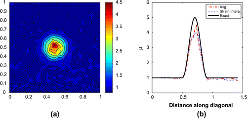
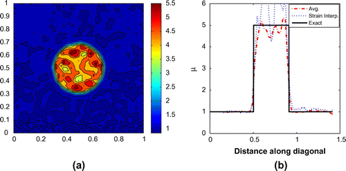
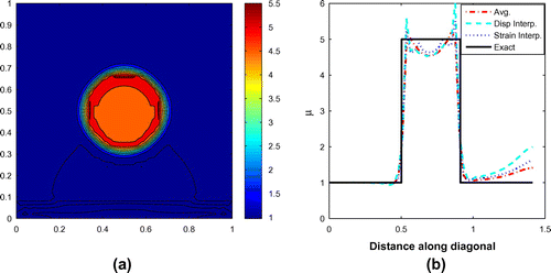
Therefore, we consider smoothing and regularization to improve the reconstruction for this noise-free but discontinuous problem. Figure 7 depicts the results obtained using smoothed data. Figure 7(a) is a contour plot obtained using the $3\times 3$ averaging procedure. Figure 7(b) presents the shear modulus distribution along the diagonal obtained using the $3\times 3$ averaging procedure and in addition, the two down-sampling and interpolation procedures. Compared to the untreated data (Figure 6), the improvement is significant. All methods show a significant improvement in the recovered contrast, and also some improvement in the background away from the inclusion. Of the three methods, the $3\times 3$ averaging procedure appears to provide the most accurate results. Of the two down-sampling and interpolation procedures, strain interpolation provides better results than displacement interpolation.

Figure 7. Stepped inclusion problem solved using smoothed data (cf. Figure 6): (a) solution in the entire region and (b) along the diagonal.

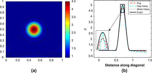
Next we apply the smoothing procedures to the smooth profiles. Although the results for the smooth profile were very accurate and no additional treatment is necessary, in practical applications a-priori knowledge about the inclusion form is usually unavailable. Therefore, we use the smooth profile as an additional test case to evaluate the effect of smoothing. Figure 8(a) is a contour plot obtained using the $3\times 3$ averaging procedure and Figure 8(b) presents the shear modulus distribution along the diagonal. The results obtained are quite accurate and close to those obtained using the unsmoothed data. We find again that $3\times 3$ averaging provides the most accurate results, followed by the strain interpolation procedure and then by the displacement interpolation. For the displacement interpolation, we find the shape of the inclusion is slightly distorted around the tip.

Figure 8. Smooth inclusion problem solved using smoothed data (cf. Figure 5): (a) solution in the entire region and (b) along the diagonal.

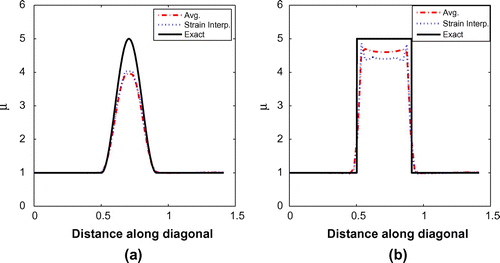
The last test we consider for the noise-free data involves a combination of smoothing and regularization. Smoothing had proven useful in recovering some of the lost contrast for the stepped inclusion problem, but the accuracy away from the calibration region is still fairly low. Considering the discussion in the appendix, the regularization parameter is set to $\mathit{\alpha }=3$ (the suggested regularization level for the stepped inclusion). Figure 9 presents the recovered material properties when regularization is applied in addition to the $3\times 3$ averaging procedure and in addition to the strain interpolation procedure (the displacement interpolation which was least accurate is no longer tested). For the stepped inclusion (Figure 9(b)), the results have further improved. The solution away from the calibration region is now accurate, and the inclusion appears more homogeneous with very little loss of contrast. The $3\times 3$ averaging procedure once more appears to provide better results than strain interpolation. For the smooth inclusion (Figure 9(a)), the results are now more accurate away from the calibration region, but about 20% of the contrast has also been diminished as a results of the regularization. The regularization level suggested in the appendix for the smooth inclusion ($\mathit{\alpha }=0.2$) is much lower than the value for the stepped inclusion which we set here. In those cases where smooth inclusions are sought, lower values should be set. When no a-priori information about the shape of the inclusion is available, the general guidelines provided in the end of the appendix can be used.

Figure 9. Inclusion problem with smoothed data and with TV regularization applied ($\mathit{\alpha }=3$): (a) reconstructed material properties for the smooth profile and (b) the stepped profile.

As we saw above, when large gradients are present in the strain data, some stabilizing influence of filtering can lead to improved performance of the AWE formulation. The same benefits may be expected when the data are corrupted by random noise, as shown in the next section.

4.3.2 Performance with noise

In practical applications, measured displacements always involve a certain amount of noise which compromises the accuracy of the solution to the inverse problem. The extent to which the solution is impaired is related to the robustness of the method used to solve the inverse problem. In this section, we evaluate the performance of the AWE method in the presence of noise. We add white Gaussian noise to the displacements such that $30\%$ noise is measured on the strains (see Figure 4). This level of noise is consistent with that found in measurements collected by ultrasound, particularly in directions perpendicular to the ultrasound beam direction and is challenging for the AWE method considering the two differentiations of the displacement field in Equations (55 $$\begin{array}{c}\hfill (2{\mathit{ϵ}}_1\nabla w_1,\nabla ·(2{\mathit{ϵ}}_1\mathit{\mu }-\mathbf{1}{p}_1))+(2{\mathit{ϵ}}_2\nabla w_1,\nabla ·(2{\mathit{ϵ}}_2\mathit{\mu }-\mathbf{1}{p}_2))=0\end{array}$$5 )–(77 $$\begin{array}{c}\hfill (-\nabla w_3,\nabla ·(2{\mathit{ϵ}}_2\mathit{\mu }-\mathbf{1}{p}_2))=0\end{array}$$7 ) (the first differentiation provides the strains).

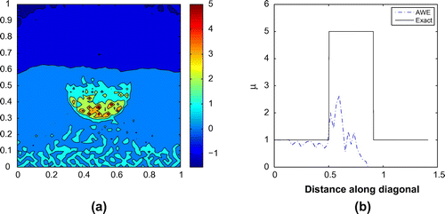
We begin by testing the AWE method without smoothing or regularization. Figures 10 and 11 depict the recovered material properties for the smooth and the stepped profiles, respectively. The solution for the the smooth profile is very poor, and the solution for the stepped profile fails completely.

Figure 10. Smooth inclusion problem with 30% noise and no treatment: (a) solution in the entire region and (b) along the diagonal.

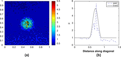
Figure 11. Stepped inclusion problem with 30% noise and no treatment: (a) solution in the entire region and (b) along the diagonal.

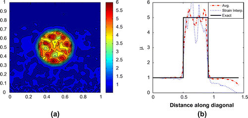
Next we apply smoothing to the noisy displacement field. Figures 12 and 13 depict the recovered material properties using $3\times 3$ averaging and strain interpolation (the contour plots are for $3\times 3$ averaging). Smoothing has introduced a dramatic improvement in the results. The improvement for the smooth profile (Figure 12) is significant and the shape and contrast are recovered fairly well. The results using the averaging procedure are more accurate than those obtained using strain interpolation, although both methods lose accuracy away from the calibration region. For the stepped profile (Figure 13), the improvement is even more significant. The results obtained using the $3\times 3$ averaging procedure are quite close to the target solution. The results obtained using strain interpolation are less accurate and involve significant oscillations inside the inclusion, but are still a significant improvement over the untreated data.

Figure 12. Smooth inclusion problem with 30% noise solved using smoothed data: (a) solution in the entire region and (b) along the diagonal.

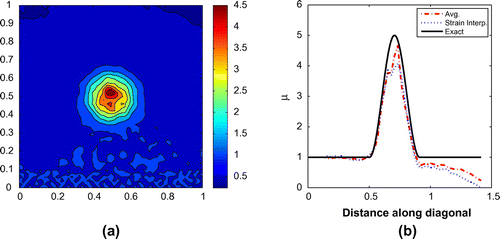
Figure 13. Stepped inclusion problem with 30% noise solved using smoothed data: (a) solution in the entire region and (b) along the diagonal.

Finally, we consider a combination of smoothing and regularization. The values suggested in the appendix for the regularization parameter in this case (stepped profile) are only slightly higher than those of the noise-free problems, so we choose again $\mathit{\alpha }=3$. The implication is that stabilizing the large strain jump in the data is more important than stabilizing against noise. Figures 14 and 15 present the recovered material properties for the smooth and the stepped profiles, respectively. For the both profiles, the results have significantly improved away from the calibration region, and are now close to the target solution. For the smooth profile, the loss in contrast is commensurate with that obtained without regularization. For the stepped profile with $3\times 3$ averaging, the regularization has dampened some of the oscillations in the inclusion. For the strain interpolation on the other hand, the oscillations remain significant.

Figure 14. Smooth inclusion problem with 30% noise solved using smoothed data and TV regularization ($\mathit{\alpha }=3$): (a) solution in the entire region and (b) along the diagonal.

Figure 15. Stepped inclusion problem with 30% noise solved using smoothed data and TV regularization ($\mathit{\alpha }=3$): (a) solution in the entire region and (b) along the diagonal.

4.4 Application to ultrasound measured deformations of a gelatin phantom

4.4.1 Gelatin phantom manufacture

A tissue-mimicking phantom was constructed from a gelatin-water-alcohol mixture to mimic the mechanical and acoustic properties of soft tissue (human breast tissue, with an approximate shear modulus of  0.5 MPa). Polyethylene granules were included to simulate the backscatter properties of soft tissue. The phantom was brick shaped with a base of $35$ mm, a height of $50$ mm and a length of $150$ mm. In the centre of the phantom, a $12$ mm diameter cylindrical inclusion, running the entire $150$ mm length, was made to mimic the relative stiffness of a tumor compared to healthy tissue. A $10$ mm calibration layer was created on top of the phantom with properties identical to those of the inclusion.

Figure 16. Photograph (Left) of cross-section of tissue-mimicking ultrasound phantom. Box shows area that was imaged. Rule is marked in mm. Horizontal (Centre) and vertical (Right) displacement estimates for compression field in ultrasound phantom. The ultrasound point spread function is highly anisotropic and provides much more precise displacement estimates in axial (vertical) direction, which is the direction of sound propagation. All values above in mm.

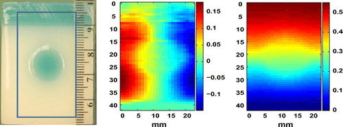
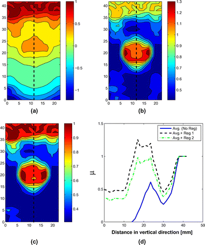
Figure 17. Reconstructed shear modulus from a gelatin phantom: (a) Solution in the entire region using averaged displacements, no regularization ($\mathit{\alpha }=0$); (b) using averaged displacements and regularization $\mathit{\alpha }=7\times {10}^{-6}$; (c) using averaged displacements and regularization $\mathit{\alpha }=3.5\times {10}^{-6}$; and (d) solution along a vertical line through the centre.

The phantom was constructed by first pouring the background gelatin into a plastic mould. The background was made with a solution that was $8\%$ by mass concentration of gelatin. The gelatin was allowed to set by cooling at 4 degrees Celsius. Portions of the plastic moulding forming the inclusion and the calibration layer were then removed. A second solution, $16\%$ by mass concentration of gelatin, was then poured to form the inclusion and calibration layer. The gel was again allowed to set at $4^{\circ }$C and the final phantom was then removed from the mould for imaging. Based on gelatin concentration, the expected shear modulus contrast between the background and inclusion is (very approximately) $4:1$.

4.4.2 Mechanical deformation and imaging

The tissue phantom was placed on a mechanical stage and deformed in small displacement increments. Pre-deformation and post-deformation radio-frequency ultrasound images were obtained on an Analogic Ultrasound Engine (AN 2300, Analogic, Peabody, MA), with a $10-12$ MHz (nominal) linear array. Ultrasound images at normal incidence, and steered to $\pm 0.1$   radians, were obtained at every displacement increment. The applied deformations were uniaxial compression under plane strain conditions, followed by a simple shear. Displacement fields were measured from the radio-frequency ultrasound images by an in-house finite element based non-rigid regularized image registration method.[34–36] The measured displacements were arranged on a structured grid of $16\times 32$ bilinear rectangular elements which was used in the computations.

4.4.3 Modulus inversion

As is typical with ultrasound measured displacements, the horizontal component of displacement (see Figure 16) is significantly noisier than the vertical component. Therefore, we apply smoothing to only the horizontal component of the measured displacement. We do so by averaging a $5\times 3$ stencil of points. The displacement data are generated using two loadings similar to those used for the synthetic data, i.e. a shear load and a compression load.

For determining the regularization parameter, we use Equation (A10) in Appendix 1, and the following choices of parameters: $U=0.8$ mm, maximum axial displacement; $L=32$ mm = the domain perimeter / 4; $\mathit{\delta }\mathit{\mu }=1=$ reference modulus in calibration strip; $h=1.36$ mm = element perimeter/4; $\overline{L}=2h$, assuming a sharp jump in properties over a distance $2h$. Further, we choose $\mathit{\eta }=0$, which assumes that stabilizing against steep property gradients dominates over steep noise gradients. These choices lead to ${\mathit{\alpha }}_1=7\times {10}^{-6}$, which is much smaller than that obtained for the synthetic data. The main reason for the decrease in magnitude is the much smaller magnitude of strains here. In order to consider the dependence of the solution on the choice of the regularization parameter, we also consider the values ${\mathit{\alpha }}_2=3.5\times {10}^{-6}$ (which results from the same choices above, except for $\mathit{\delta }\mathit{\mu }=1/2$), and $\mathit{\alpha }=0$ (i.e. no regularization).

To enforce the calibration condition, we note that Figure 16 shows the top calibration layer to be about $5$  mm tall, which is about 3 elements. We assign this region a unit shear modulus. Figure 17 presents the recovered material properties with smoothing and regularization applied. Figure 17(a)–(c) is contour plots of the solution in the entire domain, and Figure 17(d) presents a plot along a vertical line in the centre (denoted by the dashed line in the contour plot). Figure 17(a) (and the corresponding curve in Figure 17(d)) presents the reconstruction using displacement averaging only (i.e. $\mathit{\alpha }=0$, or no regularization). The results are relatively poor, probably due to loss of stability. Figure 17(b) and (c) presents the reconstruction with the regularization parameters $\mathit{\alpha }={\mathit{\alpha }}_1$ and $\mathit{\alpha }={\mathit{\alpha }}_2$, respectively. The improvement is dramatic, and a circular inclusion with elevated stiffness is clearly visible in the centre of the domain. The reconstructed inclusion has a location, size and shape consistent with the phantom manufacture and the photograph of the phantom cross-section. The stiffness contrast between the inclusion and background is about $2.8$, which is significantly below the rough $4:1$ expectation, but within range of accuracy of the rough rule of thumb provided by the concentration. More precise measures of accuracy in the reconstruction are the homogeneity of the modulus within each of the three regions, and the agreement (or lack thereof) of the reconstructed modulus within the inclusion and the calibration layer. By these measures, Figure 17(b) and (c) shows the combination of averaging and regularization has performed quite well.

5 Summary

In this work, we investigated the ability of the AWE method to recover discontinuous solutions in the presence of noise. We find that the AWE method on its own performs poorly when applied directly to problems involving 30% noise in strains. We also observe that the reconstruction of discontinuous solutions is difficult, especially away from the calibration region. These two phenomena are linked to the loss of stability in the AWE formulation when applied to discontinuous data. We considered two approaches to address this problem: smoothing the data and stabilizing the formulation by adding a regularization term. After smoothing and regularization, a significant improvement in the performance of the AWE method is observed.

We find that smoothing the displacements prior to differentiating them is crucial for obtaining acceptable results when noise levels are high. We also find that smoothing improves the contrast and the accuracy away from the calibration region for problems involving discontinuous solutions. Of the two methods considered for smoothing, averaging values of neighbouring nodes provided better results than down-sampling followed by interpolation. This is likely due to a loss of information with down-sampling.

Total variation regularization, in addition to smoothing, has also proven useful. Total variation regularization tends to rectify the degraded results observed away from the calibration region which smoothing alone does not do very well. The main advantage of the total variation regularization is when applied to stepped inclusion problems. When it is known a-priori that the solution is discontinuous, then the regularization parameters can be set fairly high, removing spurious oscillations from the solution with little compromise to the contrast. The main disadvantage of using TV regularization is that the problem becomes non-linear, significantly increasing the computational costs.

The low computational costs of direct solution approaches like the AWE make them potential candidates for real-time imaging. On the other hand, for these methods to become useful, proper adaptations for handling noise are necessary. Here, we were able to show that using relatively simple procedures, direct solutions to inverse problems of elasticity are possible even at relatively high levels on noise. Specifically, smoothing is a necessary first step for obtaining acceptable reconstructions. The use of TV regularization should be considered mainly for problems involving discontinuous solutions.

Acknowledgements

This work was supported by the United States-Israel Binational Science Foundation (BSF), Jerusalem, Israel, under Grant No. 2004400 and the National Institutes of Health under Grant No. NCI-R01CA140271.

Appendix 1

Selection of the regularization parameter

The TV regularization term appended to the AWE formulation is scaled by the regularization parameter $\mathit{\alpha }$. The choice of this parameter depends of the level of noise in the data and on the geometry of the inclusion. We propose some guidelines for choosing the TV regularization parameter by considering the length scales associated with the inverse problem considered.

Consider the AWE equation with the TV regularization term, Equation (1010 $$\begin{array}{cc}\hfill \left(2,{\mathit{ϵ}}_1,\nabla ,w_1,,,\nabla ,·,\left(2,{\mathit{ϵ}}_1,\mathit{\mu },-,\mathbf{1},p_1\right)\right)& +\left(2,{\mathit{ϵ}}_2,\nabla ,w_1,,,\nabla ,·,\left(2,{\mathit{ϵ}}_2,\mathit{\mu },-,\mathbf{1},p_2\right)\right)\hfill \\ \hfill & +\mathit{\alpha }\left(\nabla ,w_1,,,\frac{\nabla \mathit{\mu }}{\sqrt{{\left|\nabla ,\mathit{\mu }\right|}^2+{\mathit{\beta }}^2}}\right)=0\hfill \end{array}$$10 ). For simplicity, we shall use a single strain field, disregard the pressure term, and take $\mathit{\beta }$ (in the regularization term) to be zero. We use these assumptions in Equation (1010 $$\begin{array}{cc}\hfill \left(2,{\mathit{ϵ}}_1,\nabla ,w_1,,,\nabla ,·,\left(2,{\mathit{ϵ}}_1,\mathit{\mu },-,\mathbf{1},p_1\right)\right)& +\left(2,{\mathit{ϵ}}_2,\nabla ,w_1,,,\nabla ,·,\left(2,{\mathit{ϵ}}_2,\mathit{\mu },-,\mathbf{1},p_2\right)\right)\hfill \\ \hfill & +\mathit{\alpha }\left(\nabla ,w_1,,,\frac{\nabla \mathit{\mu }}{\sqrt{{\left|\nabla ,\mathit{\mu }\right|}^2+{\mathit{\beta }}^2}}\right)=0\hfill \end{array}$$10 ) and also substitute $w$ for the shear modulus, which is appropriate for the purpose of the analysis. Defining $\mathit{A}=2\mathit{ϵ}$ the equation becomes:A.1 $$\begin{array}{c}\hfill \left(\mathit{A},\nabla ,w,,,\nabla ,·,(,\mathit{A},w,)\right)+\mathit{\alpha }\int |\nabla w|d\mathrm{\Omega }\approx 0\end{array}$$A.1 Next we use Young’s inequality for the first term in (A1):A.2 $$\begin{array}{c}\hfill \left(\mathit{A},\nabla ,w,,,\nabla ,·,(,\mathit{A},w,)\right)\ge \frac{1}{2}{\Vert \mathit{A}\nabla w\Vert }^2-\frac{1}{2}{\Vert (\nabla ·\mathit{A})w\Vert }^2\end{array}$$A.2 Consider now a domain of characteristic size $L$, and assume that the measured displacement field $U_0$ is corrupted by noise of characteristic amplitude $E_0$. We define the noise fraction in the displacement as:A.3 $$\begin{array}{c}\hfill \mathit{\eta }=\frac{E_0}{U_0}\end{array}$$A.3 Assume that the sampling length scale of the noise is $\tilde{h}$. With the noise included, then $\mathit{A}$ scales as:A.4 $$\begin{array}{c}\hfill \mathit{A}\sim \mathit{ϵ}+{\mathit{ϵ}}_{noise}\sim \frac{U_0}{L}+\frac{\mathit{\eta }{U}_0}{\tilde{h}}\end{array}$$A.4 Now assume scalings:A.5 $$\begin{array}{ccc}\hfill \nabla ·\mathit{A}& \sim \hfill & \hfill \frac{U_0}{L}\left(\frac{1}{\overline{L}},+,\frac{\mathit{\eta }L}{{\tilde{h}}^2}\right)\end{array}$$A.5 A.6 $$\begin{array}{ccc}\hfill w& \sim \hfill & \hfill \mathit{\delta }\mathit{\mu }\end{array}$$A.6 A.7 $$\begin{array}{ccc}\hfill \nabla w& \sim \hfill & \hfill \frac{\mathit{\delta }\mathit{\mu }}{h}\end{array}$$A.7 Here $\mathit{\delta }\mathit{\mu }$ represents the change in the shear modulus inside the domain which can be taken as ${\mathit{\mu }}_{max}-{\mathit{\mu }}_{min}$. The parameter $\overline{L}$ denotes the ‘feature size’, i.e. the part of the domain where the shear modulus varies. If the shear modulus varies slowly, it is approximately $L$ and if it varies quickly, it is the mesh parameter $h$. Note also that $\nabla w$ is not assumed to scale with $\overline{L}$, since it is a variation.

Substituting (A2)–(A6) in (A1) gives:A.8 $$\begin{array}{ccc}\hfill \mathit{\alpha }\frac{\mathit{\delta }\mathit{\mu }}{h}& \approx \hfill & \hfill C{\left(\frac{U_0}{L}\right)}^2{\left(\frac{1}{\overline{L}},+,\frac{\mathit{\eta }L}{{\tilde{h}}^2}\right)}^2{\left(\mathit{\delta }\mathit{\mu }\right)}^2-{\left(\frac{U_0}{L}\right)}^2{\left(1,+,\frac{\mathit{\eta }L}{\tilde{h}}\right)}^2{\left(\frac{\mathit{\delta }\mathit{\mu }}{h}\right)}^2\\ & \approx \hfill & \hfill C{\left(\frac{U_0}{L}\right)}^2{\left(\mathit{\delta }\mathit{\mu }\right)}^2\left[{\left(\frac{1}{\overline{L}},+,\frac{\mathit{\eta }L}{{\tilde{h}}^2}\right)}^2,-,{\left(\frac{1}{h},+,\frac{\mathit{\eta }L}{h\tilde{h}}\right)}^2\right]\\ \hfill \mathit{\alpha }& \approx \hfill & \hfill C{\left(\frac{U_0}{L}\right)}^2\left(\mathit{\delta }\mathit{\mu }\right)\left[h,{\left(\frac{1}{\overline{L}},+,\frac{\mathit{\eta }L}{{\tilde{h}}^2}\right)}^2,-,\frac{1}{h},{\left(\frac{1}{1},+,\frac{\mathit{\eta }L}{\tilde{h}}\right)}^2\right]\end{array}$$A.8 Since $\mathit{\alpha }$ should be positive, the above shows that for sufficiently small $h$, no regularization is required, provided $\overline{L}$ is fixed and finite (i.e. does not scale with $h$). When regularization is required, it scales with the positive term in (A9). Thus, considering the positive term, we get:A.9 $$\begin{array}{ccc}\hfill \mathit{\alpha }& \approx \hfill & \hfill C{\left(\frac{U_0}{L}\right)}^2\left(\mathit{\delta }\mathit{\mu }\right)\left[h,{\left(\frac{1}{\overline{L}},+,\frac{\mathit{\eta }L}{{\tilde{h}}^2}\right)}^2\right]\\ \hfill & \approx \hfill & \hfill C{\left(\frac{U_0}{L}\right)}^2\left(\frac{\mathit{\delta }\mathit{\mu }}{L}\right)\left[\left(\frac{hL}{{\overline{L}}^2},+,2,\frac{h\mathit{\eta }{L}^2}{\overline{L}{\tilde{h}}^2},+,\frac{h{\mathit{\eta }}^2{L}^3}{{\tilde{h}}^4}\right)\right]\\ \hfill & \approx \hfill & \hfill C{\left(\frac{U_0}{L}\right)}^2\left(\frac{\mathit{\delta }\mathit{\mu }}{L}\right)\left[\left(\frac{hL}{{\overline{L}}^2},+,2,\frac{h\mathit{\eta }{L}^2}{\overline{L}{\tilde{h}}^2}\right)\right]\\ & \approx \hfill & \hfill C{\left(\frac{U_0}{L}\right)}^2\left(\frac{\mathit{\delta }\mathit{\mu }}{L}\right)\left[\frac{hL}{{\overline{L}}^2},\left(1,+,2,\frac{\mathit{\eta }L}{\tilde{h}},\frac{\overline{L}}{\tilde{h}}\right)\right]\end{array}$$A.9 Consider Equation (A10). In many cases, the noise level $\mathit{\eta }$ can be estimated based on the measuring technique used (e.g. ultrasound or MRI). In addition, $U_0$,$L$ and $\tilde{h}$ are assumed to be known. On the other hand, $\mathit{\delta }\mathit{\mu }$ and $\overline{L}$ which are associated with the solution to the problem are usually unknown a-priori and should be estimated based on the specific problem considered.

The formula in Equation (A10) can be used to determine $\mathit{\alpha }$ up to a multiplicative constant. To determine this constant, we consider a synthetically set problem with a known solution. Assume a stepped inclusion problem with a contrast of 3:1 (compared to 5:1 considered in the sample problems), with $3\times 3$ displacement averaging, and with no noise. For this problem, we have $\mathit{\eta }=0$, $U_0=1$, $L=1=50$ h, $\mathit{\delta }\mathit{\mu }=3-1=2$, $\overline{L}=2$ h (i.e. $3\times 3$ filter). Solving Equation (A10) for the regularization parameter gives $\mathit{\alpha }\approx 25C$. Next we solve the inverse problem varying the regularization parameter in (1010 $$\begin{array}{cc}\hfill \left(2,{\mathit{ϵ}}_1,\nabla ,w_1,,,\nabla ,·,\left(2,{\mathit{ϵ}}_1,\mathit{\mu },-,\mathbf{1},p_1\right)\right)& +\left(2,{\mathit{ϵ}}_2,\nabla ,w_1,,,\nabla ,·,\left(2,{\mathit{ϵ}}_2,\mathit{\mu },-,\mathbf{1},p_2\right)\right)\hfill \\ \hfill & +\mathit{\alpha }\left(\nabla ,w_1,,,\frac{\nabla \mathit{\mu }}{\sqrt{{\left|\nabla ,\mathit{\mu }\right|}^2+{\mathit{\beta }}^2}}\right)=0\hfill \end{array}$$10 ) and find that good results are obtained for $\mathit{\alpha }\approx 1.5$. We conclude that the multiplicative constant should be $C=1.5/25=0.06$

With the multiplicative constant available, we estimate the regularization coefficient for our sample problems. First, for the stepped inclusion problem (recall the contrast is 5:1) with no noise we have $\mathit{\eta }=0$, $U_0=1$, $L=1=50$ h, $\mathit{\delta }\mathit{\mu }=5-1=4$, $\overline{L}=2$ h (i.e. $3\times 3$ filter). Solving (A10) and multiplying by the constant we find that the regularization parameter is approximately $\mathit{\alpha }\approx 50C=3$. Next we consider the same problem with $30\%$ noise, i.e. $\mathit{\eta }L/h=0.3$. Again filtering using $3\times 3$, we have $\tilde{h}=2$ h which gives $\mathit{\eta }L/\tilde{h}=0.15$. Solving (A10) and multiplying by the constant, we find now that $\mathit{\alpha }\approx 64C=3.8$. This suggests that we hardly need to change the regularization parameter at all from the zero noise case which is consistent with our results.

For the smooth profile, we may take $\overline{L}=0.15$ which is approximately the range where the shear modulus varies from the background to its maximum value. Then for zero noise and no filtering, the regularization parameter is $\mathit{\alpha }\approx 3.6C=0.2$. This suggests that little to no regularization is necessary, which is consistent with our good results for the untreated AWE solution (Figure 5(a)). If we now add $30\%$ noise, the value increases to $\mathit{\alpha }\approx 20C=1.2$ which has relatively small effect, indicating that for the smooth profile the regularization should be kept fairly low at this noise level.

The formula for the regularization parameter $\mathit{\alpha }$ (Equation (A10)) contains the parameters $\tilde{h}$, $\overline{L}$, and $\mathit{\delta }\mathit{\mu }$. Of these, $\tilde{h}$ can be set equal to an estimate of the correlation length of the noise. The other two parameters $\overline{L}$ and $\mathit{\delta }\mathit{\mu }$ depend on the solution and need to be guessed. A good initial estimate for $\overline{L}=L/3$, where $L$ is the characteristic length of the domain of interest and $\mathit{\delta }\mathit{\mu }=\overline{\mathit{\mu }}$, where $\overline{\mathit{\mu }}$ is the value for the shear modulus in the calibration layer.

References

- Ophir J, Céspedes I, Ponnekanti H, Yazdi Y, Li X. Elastography: a method for imaging the elasticity of biological tissues. Ultrason. Imaging. 1991;13:111–134.
- Céspedes I, Ophir J, Ponnekanti H, Maklad NF. Elastography: elasticity imaging using ultrasound with application to muscle and breast in vivo. Ultrason. Imaging. 1993;15:73–88.
- Belaid N, Céspedes I, Thijssen J, Ophir J. Lesion detection in simulated elastographic and echographic images: a psychophysical study. Ultrasound Med. Biol. 1994;20:877–891.
- Ophir J, Céspedes I, Garra BS, Ponnekanti H, Huang Y, Maklad N. Elastography: ultrasonic imaging of tissue strain and elastic modulus in vivo. Eur. J. Ultrasound. 1996;3:49–70.
- Garra BS, Céspedes I, Ophir J, Spratt S, Zuurbier RA, Magnant CM, Pennanen MF. Elastography of breast lesions: initial clinical results. Radiology. 1997;202:79–86.
- Konofagou EE, Ophir J. Precision estimation and imaging of normal and shear components of the 3D strain tensor in elastography. Phys. Med. Biol. 2000;45:1553–1563.
- Konofagou EE, Dhooge J, Ophir J. Myocardial elastography a feasibility study in vivo. Ultrasound Med. Biol. 2002;28:475–482.
- Hoyt K, Forsberg F, Merritt CRB, Liu JB, Ophir J. In vivo elastographic investigation of ethanol induced hepatic lesions. Ultrasound Med. Biol. 2005;31:607–612.
- Righetti R, Garra BS, Mobbs LM, Kraemer-Chant CM, Ophir J, Krouskop TA. The feasibility of using poroelastography techniques for distinguishing between normal and lymphedematous tissues in vivo. Phys. Med. Biol. 2007:6525–6541.
- Evans A, Whelehan P, Thomson K, McLean D, Brauer K, Purdie C, Jordan L, Baker L, Thompson A. Quantitative shear wave ultrasound elastography: initial experience in solid breast masses. Breast Cancer Res. 2010;12.
- Van Houten EEW, Paulsen KD, Miga MI, Kennedy FE, Weaver JB. An overlapping subzone technique for MR-based elastic property reconstruction, magnetic resonance in medicine. Magnet. Reson. Med. 1999;42:779–786.
- Doyley MM, Meaney PM, Bamber JC. Evaluation of an iterative reconstruction method for quantitative elastography. Phys. Med. Biol. 2000;45:1521–1540.
- Oberai AA, Gokhale NH, Feijoo GR. Solution of inverse problems in elasticity imaging using the adjoint method. Inverse Probl. 2003;19:297–313.
- Barbone PE, Oberai AA, Harari I. Adjoint-weighted variational formulation for direct solution of inverse heat conduction problem. Inverse Probl. 2007;23:2325–2342.
- Albocher U, Oberai AA, Barbone PE, Harari I. Adjoint-weighted equation for inverse problems of incompressible plane-stress elasticity. Comput. Method. Appl. M. 2009;198:2412–2420.
- Barbone PE, Rivas CE, Harari I, Albocher U, Oberai AA, Zhang Y. Adjoint-weighted variational formulation for the direct solution of inverse problems of general linear elasticity with full interior data. Int. J. Numer. Meth. Eng. 2010;81:1713–1736.
- Zhang Y, Oberai AA, Barbone PE, Harari I. Solution of the time-harmonic viscoelastic inverse problem with interior data in two dimensions. Int. J. Numer. Meth. Eng. 2012;92:1100–1116.
- Barbone PE, Gokhale NH. Elastic modulus imaging: on the uniqueness and nonuniqueness of the elastography inverse problem in two dimensions. Inverse Probl. 2004;20:283–296.
- Franca LP, Frey SL, Hughes TJR. Stabilized finite element methods. I: Application to the advective-diffusive model. Comput. Method. Appl. M. 1992;95:253–276.
- Hughes TJR. Multiscale phenomena: Green’s functions, the Dirichlet-to-Neumann formulation, subgrid scale models, bubbles and the origins of stabilized methods. Comput. Method. Appl. M. 1995;127:387–401.
- Barbone PE, Harari I. Nearly H1-optimal finite element methods. Comput. Method. Appl. M. 2001;190:5679–5690.
- Brooks AN, Hughes TJR. Streamline upwind/Petrov-Galerkin formulations for convection dominated flows with particular emphasis on the incompressible Navier-Stokes equations. Comput. Method. Appl. M. 1982;32:199–259.
- Hughes TJR, Brooks AN. A multi-dimensional upwind scheme with no crosswind diffusion. In: Hughes TJR,editor. Finite element methods for convection dominated flows, AMD, Vol. 34. New York (NY): ASME; 1979. p. 19–35.
- Simonoff JS. Smoothing methods in statistics. New York (NY): Springer; 1996.
- Geurts BJ, Holm DD. Regularization modeling for large-eddy simulation. Phys. fluids. 2003;15:L13.
- Rudin LI, Osher S, Fatemi E. Nonlinear total variation based noise removal algorithms. Phys. D: Nonlinear Phenomena. 1992;60:259–268.
- Vogel CR, Oman ME. Fast, robust total variation-based reconstruction of noisy, blurred images. IEEE Trans. Image Process. 2002;7:813–824.
- Hughes TJR, Mallet M. A new finite element formulation for computational fluid dynamics: IV. A discontinuity-capturing operator for multidimensional advective-diffusive systems. Comput. Method. Appl. M. 1986;58:329–336.
- Tezduyar TE, Park YJ. Discontinuity-capturing finite element formulations for nonlinear convection-diffusion-reaction equations. Comput. Method. Appl. M. 1986;59:307–325.
- Galeao AC. Dutra do Carmo EG. A consistent approximate upwind Petrov-Galerkin method for convection-dominated problems. Comput. Method. Appl. M. 1988;68:83–95.
- Codina R. A discontinuity-capturing crosswind-dissipation for the finite element solution of the convection-diffusion equation. Comput. Method. Appl. M. 1993;110:325–342.
- Vogel CR. Computational methods for inverse problems. Philadelphia (PA): Society for industrial and applied mathematics; 2002.
- Hughes TJR. The finite element method. Mineola (NY): Dover; 2000.
- Richards MS. Quantitative three dimensional elasticity imaging [PhD thesis]. Boston (MA): Boston University; 2007.
- Richards MS, Barbone PE, Oberai AA. Quantitative three dimensional elasticity imaging from quasi-static deformation: a phantom study. Phys. Med. Biol. 2009;54:757–779.
- Richards MS, Doyley MM. Non-rigid image registration based strain estimator for intravascular ultrasound elastography. Ultrasound Med. Biol. 2013;39:515–533.