Parametric identification of a heating mobile source in a three-dimensional geometry

Abstract

The resolution of an inverse problem of heat conduction in a three-dimensional plate using an iterative regularization method based on Alifanov’s iterative regularization method is investigated. Considering temperature observation on the upper face centre of a small thin steel plate, the time dependent strength of a plane heat source has to be identified. Two configurations are studied. For the first one, the heat source is fixed on the lower face centre. For the second one, the heat source is mobile and the trajectory is assumed to be known. For both situations, robustness of the approach is stated considering noisy measurements.

Keywords:

• inverse heat conduction problem
• mobile source identification
• conjugate gradient method

1. Introduction

For several decades, resolution of inverse problems in thermal sciences is a key-goal in numerous engineering applications. Related literature is quite wide since applications deal with different geometries and configurations for many identification purposes like initial conditions [1], boundary exchange coefficient [2], thermal parameters[3] or heat source characterization. In this last framework, several applications are investigated in recent references: control of welding processes using nonintrusive observations [4,5]; prediction of the thermal effect of High Energy Laser (HEL) weapons, in order to predict the potential damage on a target [6] and estimation of temperature in human tissues submitted to a laser occurrence.[7] During the two past decades, several studies have been investigated from one-dimensional geometry [8] to two-dimensional geometries (see [9–11]). It is well known that such inverse problems are ill-posed.[12,13] Several approaches can be implemented to deal with parametric identification: singular value decomposition [13], Tikhonov regularization [14] and function specification.[15] The Alifanov’s iterative regularization method has been successfully implemented in [16]. However, three-dimensional configurations are scarcely investigated due to important CPU time required for identification purposes (in [17–22] parametric identification in a thermal context is investigated). Nowadays, heat flux identification still remains a lively research topic (see recent references [23–26]).

In the following, identification of timewise-varying strength of a fixed or mobile heating source is investigated. The spatial distribution of the source is assumed to be a disc which is moved on the lower surface of a plane-parallel sample. A sensor located on the upper surface provides temperature observations for identification purposes. Two configurations are studied: for the first one, the source is fixed; while for the second one, its trajectory is circular.

This communication is organized as follows. In the next section, the studied thermal process is modelled and numerical resolutions of the direct problem (considering finite element method implemented with Comsol Multiphysics™ and Matlab® softwares) are presented and analysed. In the third section, inverse problem is investigated: inverse heat conduction problem is formulated and conjugate gradient algorithm is presented. For these minimization methods, resolution of three well-posed problems is required: direct problem (for quadratic cost function estimation), adjoint problem (for cost function gradient computation) and sensitivity problem (for descent depth estimation). In this section, the stop criterion is also discussed. Then numerical implementation is performed and analysed in section four. Several configurations are studied in order to estimate the identification efficiency: fixed and mobile source with or without noise on measurements. In the last section, experimental results are analysed. Then, concluding remarks and several outlooks are proposed in the last section.

2. Direct problem

In this section, the direct thermal problem is described and the studied partial differential equation system is defined. When all the parameters (model inputs) are given, numerical resolution of such problem leads to the determination of the temperature evolution at each point of the investigated domain.

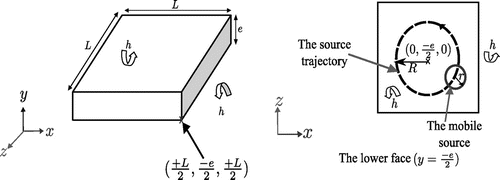
Let us consider a square plate $\mathrm{\Omega }$ (thickness is denoted by $e$ and length is denoted by $L$). The space variables are $(x,y,z)\in \mathrm{\Omega }=]\frac{-L}{2},\frac{L}{2}[\times ]\frac{-e}{2},\frac{e}{2}[\times ]\frac{-L}{2},\frac{L}{2}[$, while the time variable is $t\in T=[0,t_f]$; boundary of $\mathrm{\Omega }$ is denoted by $\mathit{\partial }\mathrm{\Omega }$ and $\mathit{\theta }(x,y,z;t)$ is the temperature in Kelvin. The studied three-dimensional sample is heated on its lower face ${\mathrm{\Gamma }}_{heated}=\{(x,\frac{-e}{2},z)\in \mathit{\partial }\mathrm{\Omega }\}$ considering a mobile (or fixed) source assumed to be uniform on a disc $D$: radius $r=2{10}^{-3}$ m, centre $I(t)$. Then, the heating flux $\mathrm{\Phi }(x,y,z;t)$ is defined as follows:$$\mathrm{\Phi }(x,y,z;t)=\left\{\begin{array}{cc}\mathit{\varphi }(t)\hfill & \text{if}\left(x,-\frac{e}{2},z\right)\in D(I(t),r)\hfill \\ 0\hfill & \text{else}\hfill \end{array}\right.$$

This heating flux expression can also be written as follows:$$\mathrm{\Phi }(x,z;t)\approx -\frac{\mathit{\varphi }(t)}{\mathit{\pi }}\left(\text{atan}\left(\mathit{\mu }\sqrt{{(x-X(t))}^2+{(z-Z(t))}^2}-\mathit{\mu }r\right)-\frac{\mathit{\pi }}{2}\right)$$

where $(X(t),Z(t))$ are the centre source coordinates at time $t$ and $\mathit{\mu }>0$ is a positive constant arbitrarily chosen in order to describe the spatial discontinuity on disc boundary. Let us consider a circular trajectory such that $I(t)=(Rcos(\mathit{\omega }t),\frac{-e}{2},Rsin(\mathit{\omega }t))$ on the lower surface where $R$ is the trajectory radius in $(\text{m})$ and $\mathit{\omega }$ is the angular velocity in $(\text{rad/s})$. Moreover, natural convection is considered on $\mathit{\partial }\mathrm{\Omega }$, convection coefficient is $h$ in $(\text{W}{\text{m}}^{\text{- 2}}{\text{K}}^{-1})$. The considered three-dimensional geometry is presented in Figure 1.

Figure 1. Three-dimensional geometry.

Considering the initial uniform temperature ${\mathit{\theta }}_0$ (equal to the ambient temperature) and the set of the known parameters $\{\mathit{\lambda },\mathit{\rho }c,h,\mathrm{\Phi },L,e\}$, the direct problem resolution aims to find the temperature $\mathit{\theta }(x,y,z;t)$ which satisfies:(1) $$\left\{\begin{array}{cc}\mathit{\lambda }\left(\frac{{\mathit{\partial }}^2\mathit{\theta }(.)}{\mathit{\partial }{x}^2}+\frac{{\mathit{\partial }}^2\mathit{\theta }(.)}{\mathit{\partial }{y}^2}+\frac{{\mathit{\partial }}^2\mathit{\theta }(.)}{\mathit{\partial }{z}^2}\right)=\mathit{\rho }c\frac{\mathit{\partial }\mathit{\theta }(.)}{\mathit{\partial }t}\hfill & \forall (x,y,z;t)\in \mathrm{\Omega }\times T\hfill \\ \mathit{\theta }(x,y,z;0)={\mathit{\theta }}_0\hfill & \forall (x,y,z)\in \mathrm{\Omega }\hfill \\ -\mathit{\lambda }\frac{\mathit{\partial }\mathit{\theta }(.)}{\mathit{\partial }\overrightarrow{n}}=h(\mathit{\theta }(.)-{\mathit{\theta }}_0)-\mathrm{\Phi }(x,y,z;t)\hfill & \forall (x,y,z;t)\in \mathit{\partial }\mathrm{\Omega }\times T\hfill \end{array}\right.$$(1)

In order to highlight the three-dimensional heat transfer, a thermal insulating material is chosen (a glass plate). All the input parameters are presented in the following table and figure.

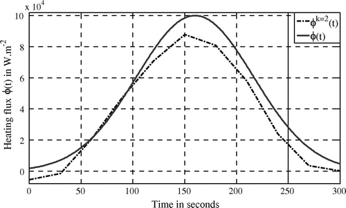
Heating flux $\mathit{\varphi }(t)$ is $\mathit{\varphi }(t)={10}^{5}exp\left(-{\left(\frac{t-160}{80}\right)}^2\right)$; see Figure 2.

Figure 2. Heating flux $\mathit{\varphi }(t)$.

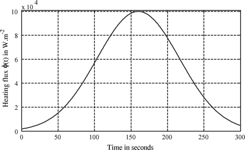
Based on the previous Equation (1$$\mathrm{\Phi }(x,y,z;t)=\left\{\begin{array}{cc}\mathit{\varphi }(t)\hfill & \text{if}\left(x,-\frac{e}{2},z\right)\in D(I(t),r)\hfill \\ 0\hfill & \text{else}\hfill \end{array}\right.$$), the set of parameters (Table 1) and the heating flux strength (Figure 2), the direct problem can be solved using finite element method implemented with Comsol Multiphysics^TM solver and Matlab® software. Two numerical examples are presented hereafter: the first one corresponds to a fixed source, while the second one describes a mobile source (circular trajectory).

Table 1. Parameters for direct problem resolution.

Square length $L$ in m	Plate thickness $e$ in m	Initial temperature ${\mathit{\theta }}_0$ in K	Final time $t_f$ in s
$5\times {10}^{-2}$	$2\times {10}^{-3}$	293	300
Thermal conductivity $\mathit{\lambda }$ in $\text{W}{\text{m}}^{\text{- 1}}{\text{K}}^{-1}$	Volumetric heat capacity $\mathit{\rho }c$ in $\text{J}{\text{m}}^{\text{- 3}}{\text{K}}^{-1}$	Natural convection coefficient $h$ in $\text{W}{\text{m}}^{\text{- 2}}{\text{K}}^{-1}$
1.2	$2\times {10}^6$	20

Table 2. Cost function values for several iterations (fixed source).

Iteration k	0	1	2	3	4	5	6
$J({\mathit{\varphi }}^k)$	827,622	10,709	646	489	360	184	149
$Err$	182,812	26,066	8530	5974	4180	2322	2440

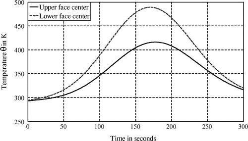
For a fixed source located on the centre of the lower face (corresponding to an axisymmetric configuration), temperature evolution issued from the direct problem resolution is presented in Figure 3 for the centre of both lower and upper faces.

Figure 3. Temperature evolution for the fixed heating source (direct problem).

For a mobile source ($R=2\times {10}^{-2}\text{m}$, $\mathit{\omega }=\frac{2\mathit{\pi }}{300}\text{rad}{\text{s}}^{-1}$), temperature evolution is shown for several points $C_{j=1,\dots ,5}$ located on the upper face (see Figure 4).

Figure 4. Sensors’ locations (upper face) and source trajectory (lower face).

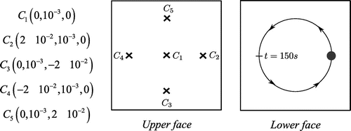
In Figure 5, it is shown that the highest temperature, obtained at point $C_4$ at $t=154\text{s}$ is equal to $\mathit{\theta }(C_4,154)=372.6\text{K}$. Such result is obviously in adequacy with the heating flux which is high at $t=154\text{s}$ (see Figure 3) and located near point $C_4$.

Figure 5. Temperature evolution on the upper face (mobile source – direct problem).

In the following section, identification of the unknown heating flux considering temperature observations is investigated (a single point located in the upper face centre is considered). Then, for the fixed source thermogram presented in Figure 3, (continuous line) is taken into account while for the mobile source temperature observed at point $C_1$ is considered (Figure 5). Temperature is assumed to be measured each second (then 300 observations are available for heat flux identification).

3. Inverse problem

3.1. Alifanov’s iterative regularization method

Let us consider that the strength heating flux of the fixed or the mobile source is unknown and denoted $({\mathit{\varphi }}^{\ast }(t))$. In order to estimate this unknown parameter, a three-dimensional inverse heat conduction problem (3D-IHCP) is formulated as a classical optimization problem which consists in the minimization of a quadratic criterion denoted by $J(\mathit{\varphi }(t),\mathit{\theta })$. This criterion describes the quadratic difference between the simulated temperature (solution of direct problem (1)) and the measured temperature $\widehat{\mathit{\theta }}(t)$ obtained at sensor $C_1$.

Thus, the identification problem can be formulated as an inverse one:

Find the unknown heating flux ${\mathit{\varphi }}^{\ast }(t)$ such that the following quadratic functional $J(\mathit{\varphi })$ is minimal: (2) $${\mathit{\varphi }}^{\ast }(t)=\underset{\mathit{\varphi }\in L^2(T)}{\text{Arg}min}J(\mathit{\varphi })=\underset{\mathit{\varphi }\in L^2(T)}{\text{Arg}min}\frac{1}{2}{\int }_0^{t_f}{\left(\mathit{\theta }\left(0,\frac{e}{2},0;t;\mathit{\varphi }\right)-\widehat{\mathit{\theta }}(t)\right)}^{2}dt$$(2)

with the constraint $\mathit{\theta }(x,y,z;t;\mathit{\varphi })$ solution of the direct problem (1).

The functional space is defined as the space of quadratically integrable functions on $T$: $L^2(T)=\{\mathit{\varphi }/{\int }_T{\mathit{\varphi }}^2(t)dt<+\infty \}$. Usually, a parameterization of the functional $\mathit{\varphi }(t)$ is proposed and without lack of generalities let us consider continuous piecewise linear function. Thus, in the following, heating flux is assumed to be defined $\forall t\in T=[0300]$ on $N_t=10$ time intervals $I_n=[p_{n-1},p_n]=[30(n-1),30n]$ with $n=1,\dots ,10$ and time step duration $\mathit{\tau }=p_n-p_{n-1}=30\text{s}$ by $\mathit{\varphi }(t)={\sum }_{i=1}^{11}{\mathit{\varphi }}_i{s}_i(t)=\overline{\mathit{\varphi }}\dots {\overline{s(t)}}^{tr}$ where $\overline{\mathit{\varphi }}=({\mathit{\varphi }}_1,\cdots ,{\mathit{\varphi }}_{11})\in {\mathbb{R}}^{11}$, $\overline{s(t)}=(s_1(t),\cdots ,s_{11}(t))$ and $tr$ is the transpose operator. The basis functions $s_i(t)$ are:$$s_i(t)=\left\{\begin{array}{cc}\frac{t-p_{i-2}}{\mathit{\tau }}& \text{if}t\in [p_{i-2},p_{i-1}]\\ \frac{p_i-t}{\mathit{\tau }}& \text{if}t\in [p_{i-1},p_i]\\ 0& \text{elsewhere}\end{array}\right..$$

In Figure 6, basis functions $s_i(t)$ are drawn.

Figure 6. Basis functions $s_i(t)$.

Discrete formulation of the inverse problem leads to determine the unknown heating flux(3) $${\overline{\mathit{\varphi }}}^{\ast }={({\mathit{\varphi }}_i^{\ast })}_{i=1,\cdots ,11}=\underset{\overline{\mathit{\varphi }}\in {\mathbb{R}}^{11}}{\text{Arg}min}J(\overline{\mathit{\varphi }})=\underset{\overline{\mathit{\varphi }}\in {\mathbb{R}}^{11}}{\text{Arg}min}\frac{1}{2}{\int }_0^{t_f}{\left(\mathit{\theta }\left(0,\frac{e}{2},0;t;\overline{\mathit{\varphi }}\right)-\widehat{\mathit{\theta }}(t)\right)}^{2}dt$$(3)

with the constraint $\mathit{\theta }(x,y,z,t;\overline{\mathit{\varphi }})$ solution of the direct problem $(1)$.

In order to solve the previous ill-posed problem, Alifanov’s iterative regularization method is implemented. In this communication, a conjugate gradient method (see for example [8,14,27]) is proposed with an adjoint equation that leads to the gradient. Such algorithm leads to the iterative numerical resolution of three well-posed problems. At each iteration $k$

• Resolution of the direct problem (1) and criterion computation $J({\overline{\mathit{\varphi }}}^k)$.

• Resolution of an adjoint problem in order to estimate cost function gradient ${\left(\frac{\mathit{\partial }J}{\mathit{\partial }{\overline{\mathit{\varphi }}}_i^k}\right)}_{i=1,\cdots ,11}$ and to determine the descent direction ${\overline{d}}^k$.

• Resolution of the sensitivity problem (in the descent direction) in order to estimate descent depth ${\mathit{\gamma }}^k$.

More details are given on such procedure in [9,10,19,28]. Direct problem resolution using finite element solver has been presented in previous section. In the following, sensitivity problem and adjoint problem are formulated.

3.2. Sensitivity problem

This problem consists in the determination of the temperature variation $\mathit{\delta }\mathit{\theta }(x,y,z;t)$ induced by a variation of the unknown function $\mathit{\delta }\mathit{\varphi }(t)={\sum }_{i=1}^{11}(\mathit{\delta }{\mathit{\varphi }}_i)s_i(t)$ (applications of variational calculus are presented in [29]). Considering the partial differential equations system satisfied by the temperature $\mathit{\theta }(x,y,z;t)+\mathit{\epsilon }\mathit{\delta }\mathit{\theta }(x,y,z;t)$ (see direct problem (1) with an heating flux $\mathit{\varphi }(t)+\mathit{\epsilon }\mathit{\delta }\mathit{\varphi }(t)$) then while $\mathit{\epsilon }\to 0$, the sensitivity problem [9,10] becomes:(4) $$\left\{\begin{array}{cc}\mathit{\lambda }\left(\frac{{\mathit{\partial }}^2\mathit{\delta }\mathit{\theta }(.)}{\mathit{\partial }{x}^2}+\frac{{\mathit{\partial }}^2\mathit{\delta }\mathit{\theta }(.)}{\mathit{\partial }{y}^2}+\frac{{\mathit{\partial }}^2\mathit{\delta }\mathit{\theta }(.)}{\mathit{\partial }{z}^2}\right)=\mathit{\rho }c\frac{\mathit{\partial }\mathit{\delta }\mathit{\theta }(.)}{\mathit{\partial }t}\hfill & \forall (x,y,z;t)\in \mathrm{\Omega }\times T\hfill \\ \mathit{\delta }\mathit{\theta }(x,y,z;0)=0\hfill & \forall (x,y,z)\in \mathrm{\Omega }\hfill \\ -\mathit{\lambda }\frac{\mathit{\partial }\mathit{\delta }\mathit{\theta }(.)}{\mathit{\partial }\overrightarrow{n}}=h\mathit{\delta }\mathit{\theta }(.)-\mathit{\delta }\mathrm{\Phi }(.)\hfill & \forall (x,y,z;t)\in \mathit{\partial }\mathrm{\Omega }\times T\hfill \end{array}\right.$$(4)

In the studied configuration, the heating flux variation $\mathit{\delta }\mathrm{\Phi }(x,y,z;t)$ is:$$\mathit{\delta }\mathrm{\Phi }(x,y,z;t)=\left\{\begin{array}{cc}\mathit{\delta }\mathit{\varphi }(t)={\sum }_{i=1}^{11}(\mathit{\delta }{\mathit{\varphi }}_i)s_i(t)=\mathit{\delta }\overline{\mathit{\varphi }}·{\overline{s(t)}}^{tr}\hfill & \text{if}\left(x,-\frac{e}{2},z\right)\in D(I(t),r)\hfill \\ 0\hfill & \text{else}\hfill \end{array}\right.$$

The analytical expression of the heat flux variation is:$$\mathit{\delta }\mathrm{\Phi }(x,z;t)=-\frac{\mathit{\delta }\mathit{\varphi }(t)}{\mathit{\pi }}\left(\text{atan}\left(\mathit{\mu }\sqrt{{(x-X(t))}^2+{(z-Z(t))}^2}-\mathit{\mu }r\right)-\frac{\mathit{\pi }}{2}\right)$$

Using the sensitivity problem formulation, the descent depth can be easily formulated. At each iteration $k$, descent depth ${\mathit{\gamma }}^k$ is a real value corresponding to the optimal depth for the new value of the unknown heating flux ${\overline{\mathit{\varphi }}}^{k+1}={\overline{\mathit{\varphi }}}^k-{\mathit{\gamma }}^k{\overline{d}}^k$. Thus, it is defined as:(5) $${\mathit{\gamma }}^k=\underset{\mathit{\gamma }\in {\mathbb{R}}^{*}}{\text{Arg}min}J({\overline{\mathit{\varphi }}}^k-\mathit{\gamma }{\overline{d}}^k)=\underset{\mathit{\gamma }\in {\mathbb{R}}^{*}}{\text{Arg}min}\frac{1}{2}{\int }_0^{t_f}{(\mathit{\theta }(C_1;t;{\overline{\mathit{\varphi }}}^k-\mathit{\gamma }{\overline{d}}^k)-\widehat{\mathit{\theta }}(t))}^{2}dt$$(5)

Then, (6) $${\mathit{\gamma }}^k=\frac{{\int }_0^{t_f}(\mathit{\theta }(C_1;t;{\overline{\mathit{\varphi }}}^k)-\widehat{\mathit{\theta }}(t))\mathit{\delta }{\mathit{\theta }}_{{\overline{d}}^k}(C_1;t)dt}{{\int }_0^{t_f}{(\mathit{\delta }{\mathit{\theta }}_{{\overline{d}}^k}(C_1;t))}^{2}dt}$$(6)

Then, at each iteration $k$, the sensitivity problem has to be solved in the descent direction ${\overline{d}}^k$ to compute the descent depth ${\mathit{\gamma }}^k$. In order to compute the descent direction ${\overline{d}}^k$, an adjoint problem is formulated.

3.3. Adjoint problem

The aim of this problem is to introduce an adjoint function $\mathit{\psi }(x,y,z;t)$ in order to determine the gradient $\overrightarrow{\mathrm{\nabla }J}=\overrightarrow{\text{grad}J(\overline{\mathit{\varphi }})}={\left(\frac{\mathit{\partial }J}{\mathit{\partial }{\mathit{\varphi }}_i}\right)}_{i=1,\dots ,11}$ and then deduce the descent direction ${\overline{d}}^{k+1}={\overrightarrow{\mathrm{\nabla }J}}^k+{\mathit{\beta }}^k{\overline{d}}^k$ (with: ${\mathit{\beta }}^k=||{\overrightarrow{\mathrm{\nabla }J}}^k{||}^2||{\overrightarrow{\mathrm{\nabla }J}}^{k+1}{||}^2$, β^k=0 = 0 and ||.|| is the Euclidian norm). This step is essential for CGM implementation (cf. e.g. in [9,10,18,19,28]). Let $\ell (\mathit{\theta },\mathit{\varphi }(t),\mathit{\psi })$ be the Lagrangian associated to the direct problem defined in (1):(7) $$\ell (\mathit{\theta },\mathit{\varphi }(t),\mathit{\psi })=J(\mathit{\theta },\mathit{\varphi })+{\int }_0^{t_f}{\int }_{\mathrm{\Omega }}\left(\mathit{\rho }c\frac{\mathit{\partial }\mathit{\theta }(.)}{\mathit{\partial }t}-\mathit{\lambda }\mathrm{\Delta }\mathit{\theta }(.)\right)\mathit{\psi }(.)dtd\mathrm{\Omega }$$(7)

Let us consider: $\mathit{\delta }\ell (\mathit{\theta },\mathit{\varphi }(t),\mathit{\psi })=\frac{\mathit{\partial }\ell }{\mathit{\partial }\mathit{\theta }}\mathit{\delta }\mathit{\theta }+\frac{\mathit{\partial }\ell }{\mathit{\partial }\mathit{\varphi }}\mathit{\delta }\mathit{\varphi }+\frac{\mathit{\partial }\ell }{\mathit{\partial }\mathit{\psi }}\mathit{\delta }\mathit{\psi }$.

• If $\mathit{\theta }$ is solution of (1), then $\ell (\mathit{\theta },\mathit{\varphi }(t),\mathit{\psi })=J(\mathit{\theta },\mathit{\varphi }(t))$ and $\mathit{\delta }\ell (\mathit{\theta },\mathit{\varphi }(t),\mathit{\psi })=\mathit{\delta }J(\mathit{\theta },\mathit{\varphi }(t))$,

• If $\mathit{\psi }$ is fixed, then $\frac{\mathit{\partial }\ell }{\mathit{\partial }\mathit{\psi }}\mathit{\delta }\mathit{\psi }=0$ and $\mathit{\delta }\ell (\mathit{\theta },\mathit{\varphi }(t),\mathit{\psi })=\frac{\mathit{\partial }\ell }{\mathit{\partial }\mathit{\theta }}\mathit{\delta }\mathit{\theta }+\frac{\mathit{\partial }\ell }{\mathit{\partial }\mathit{\varphi }}\mathit{\delta }\mathit{\varphi }$.

Then, the choice of the fixed Lagrange multiplier $\mathit{\psi }$ is performed in order to satisfy the following equation:(8) $$\frac{\mathit{\partial }\ell }{\mathit{\partial }\mathit{\theta }}\mathit{\delta }\mathit{\theta }=0,\forall \mathit{\delta }\mathit{\theta }$$(8)

In order to determine a fixed $\mathit{\psi }(x,y,z;t)$ which satisfy (8), let us formulate $\mathit{\delta }\ell (\mathit{\theta },\mathit{\varphi }(t),\mathit{\psi })$ considering (7):(9) $$\mathit{\delta }\ell (\mathit{\theta },\mathit{\varphi }(t),\mathit{\psi })={\int }_0^{t_f}{\int }_{\mathrm{\Omega }}(\mathit{\theta }(.)-\widehat{\mathit{\theta }}(.))\mathit{\delta }\mathit{\theta }(.){\mathit{\delta }}_{Dirac}(C_1)dtd\mathrm{\Omega }+{\int }_0^{t_f}{\int }_{\mathrm{\Omega }}\left(\mathit{\rho }c\frac{\mathit{\partial }\mathit{\delta }\mathit{\theta }(.)}{\mathit{\partial }t}-\mathit{\lambda }\mathrm{\Delta }\mathit{\delta }\mathit{\theta }(.)\right)\mathit{\psi }(.)dtd\mathrm{\Omega }$$(9)

where δ_Dirac(C₁) is the Dirac distribution considered on sensor position C₁. Let $E(x,y,z;t)$ the error function expressed by:$$E(x,y,z;t)=(\mathit{\theta }(x,y,z;t)-\widehat{\mathit{\theta }}(t)){\mathit{\delta }}_{Dirac}(C_1).$$

Equation (9$$\mathit{\delta }\mathrm{\Phi }(x,z;t)=-\frac{\mathit{\delta }\mathit{\varphi }(t)}{\mathit{\pi }}\left(\text{atan}\left(\mathit{\mu }\sqrt{{(x-X(t))}^2+{(z-Z(t))}^2}-\mathit{\mu }r\right)-\frac{\mathit{\pi }}{2}\right)$$) becomes:(10) $$\mathit{\delta }\ell (\mathit{\theta },\mathit{\varphi }(t),\mathit{\psi })={\int }_0^{t_f}{\int }_{\mathrm{\Omega }}E(.)\mathit{\delta }\mathit{\theta }(.)dtd\mathrm{\Omega }+{\int }_0^{t_f}{\int }_{\mathrm{\Omega }}\left(\mathit{\rho }c\frac{\mathit{\partial }\mathit{\delta }\mathit{\theta }(.)}{\mathit{\partial }t}-\mathit{\lambda }\mathrm{\Delta }\mathit{\delta }\mathit{\theta }(.)\right)\mathit{\psi }(.)dtd\mathrm{\Omega }$$(10)

Considering the integral by parts and using the Green theorem [29], the Lagrangian variation is:$$\mathit{\delta }\ell (\mathit{\theta },\mathit{\varphi }(t),\mathit{\psi })={\int }_0^{t_f}{\int }_{\mathrm{\Omega }}E(.)\mathit{\delta }\mathit{\theta }(.)dtd\mathrm{\Omega }+{\int }_{\mathrm{\Omega }}\mathit{\rho }c\mathit{\delta }\mathit{\theta }(.;t_f)\mathit{\psi }(.;t_f)d\mathrm{\Omega }-{\int }_{\mathrm{\Omega }}\mathit{\rho }c\mathit{\delta }\mathit{\theta }(.;0)\mathit{\psi }(.;0)d\mathrm{\Omega }-{\int }_0^{t_f}{\int }_{\mathrm{\Omega }}\mathit{\rho }c\frac{\mathit{\partial }\mathit{\psi }(.)}{\mathit{\partial }t}\mathit{\delta }\mathit{\theta }(.)d\mathrm{\Omega }dt-{\int }_0^{t_f}{\int }_{\mathrm{\Omega }}\mathit{\lambda }\mathit{\delta }\mathit{\theta }(.)\mathrm{\Delta }\mathit{\psi }(.)d\mathrm{\Omega }dt+{\int }_0^{t_f}{\int }_{\mathit{\partial }\mathrm{\Omega }}\mathit{\lambda }\mathit{\delta }\mathit{\theta }(.)\frac{\mathit{\partial }\mathit{\psi }(.)}{\mathit{\partial }\overrightarrow{n}}d\mathit{\partial }\mathrm{\Omega }dt-{\int }_0^{t_f}{\int }_{\mathit{\partial }\mathrm{\Omega }\mathit{\lambda }\mathit{\psi }(.)}\frac{\mathit{\partial }\mathit{\delta }\mathit{\theta }(.)}{\mathit{\partial }\overrightarrow{n}}d\mathit{\partial }\mathrm{\Omega }dt$$

Previous expression of δ$\ell$(.) is simplified considering sensitivity Equation (4(2) $${\mathit{\varphi }}^{\ast }(t)=\underset{\mathit{\varphi }\in L^2(T)}{\text{Arg}min}J(\mathit{\varphi })=\underset{\mathit{\varphi }\in L^2(T)}{\text{Arg}min}\frac{1}{2}{\int }_0^{t_f}{\left(\mathit{\theta }\left(0,\frac{e}{2},0;t;\mathit{\varphi }\right)-\widehat{\mathit{\theta }}(t)\right)}^{2}dt$$(2) ):(11) $$\mathit{\delta }\ell (\mathit{\theta },\mathit{\varphi }(t),\mathit{\psi })={\int }_0^{t_f}{\int }_{\mathrm{\Omega }}\left(E(.)-\mathit{\rho }c\frac{\mathit{\partial }\mathit{\psi }(.)}{\mathit{\partial }t}-\mathit{\lambda }\mathrm{\Delta }\mathit{\psi }(.)\right)\mathit{\delta }\mathit{\theta }(.)dtd\mathrm{\Omega }+{\int }_{\mathrm{\Omega }}\mathit{\rho }c\mathit{\delta }\mathit{\theta }(.;t_f)\mathit{\psi }(.;t_f)d\mathrm{\Omega }+{\int }_0^{t_f}{\int }_{\mathit{\partial }\mathrm{\Omega }}\mathit{\lambda }\mathit{\delta }\mathit{\theta }(.)\frac{\mathit{\partial }\mathit{\psi }(.)}{\mathit{\partial }\overrightarrow{n}}d\mathit{\partial }\mathrm{\Omega }dt+{\int }_0^{t_f}{\int }_{\mathit{\partial }\mathrm{\Omega }}h\mathit{\delta }\mathit{\theta }(.)\mathit{\psi }(.)d\mathit{\partial }\mathrm{\Omega }dt-{\int }_0^{t_f}{\int }_{{\mathrm{\Gamma }}_{heated}}\mathit{\delta }\mathrm{\Phi }(.)\mathit{\psi }(.)d\mathit{\partial }\mathrm{\Omega }dt$$(11)

In order to satisfy (8) and considering (9), let us introduce the adjoint problem satisfied by $\mathit{\psi }(x,y,z;t)$ such as:(12) $$\left\{\begin{array}{c}\mathit{\rho }c\frac{\mathit{\partial }\mathit{\psi }(.)}{\mathit{\partial }t}+\mathit{\lambda }\left(\frac{{\mathit{\partial }}^2\mathit{\psi }(.)}{\mathit{\partial }{x}^2}+\frac{{\mathit{\partial }}^2\mathit{\psi }(.)}{\mathit{\partial }{y}^2}+\frac{{\mathit{\partial }}^2\mathit{\psi }(.)}{\mathit{\partial }{z}^2}\right)=E(.)\forall (x,y,z;t)\in \mathrm{\Omega }\times T\hfill \\ \mathit{\psi }(x,y,z;t_f)=0\forall (x,y,z)\in \mathrm{\Omega }\hfill \\ -\mathit{\lambda }\frac{\mathit{\partial }\mathit{\psi }(.)}{\mathit{\partial }\overrightarrow{n}}=h\mathit{\psi }(.)\forall (x,y,z;t)\in \mathit{\partial }\mathrm{\Omega }\times T\hfill \end{array}\right.$$(12)

If $\mathit{\psi }(x,y,z;t)$ is solution of adjoint problem (12) then (11) becomes:(13) $$\begin{array}{c}\mathit{\delta }\ell (\mathit{\theta },\mathit{\varphi }(t),\mathit{\psi })=-{\int }_0^{t_f}{\int }_{{\mathrm{\Gamma }}_{heated}}\mathit{\delta }\mathrm{\Phi }(x,z;t)\mathit{\psi }(x,y,z;t)d\mathit{\partial }\mathrm{\Omega }dt\\ ={\int }_0^{t_f}{\int }_{{\mathrm{\Gamma }}_{heated}}\frac{\mathit{\delta }\mathit{\varphi }(t)}{\mathit{\pi }}\left(\text{atan}\left(\mathit{\mu }\sqrt{{(x-X(t))}^2+{(z-Z(t))}^2}-\mathit{\mu }r\right)-\frac{\mathit{\pi }}{2}\right)\mathit{\psi }(.)d\mathit{\partial }\mathrm{\Omega }dt\\ ={\sum }_{i=1}^{11}\left(\mathit{\delta }{\mathit{\varphi }}_i{\int }_0^{t_f}{\int }_{{\mathrm{\Gamma }}_{heated}}\frac{s_i(t)}{\mathit{\pi }}\left(\text{atan}\left(\mathit{\mu }\sqrt{{(x-X(t))}^2+{(z-Z(t))}^2}-\mathit{\mu }r\right)-\frac{\mathit{\pi }}{2}\right)\mathit{\psi }(.)d\mathit{\partial }\mathrm{\Omega }dt\right)\end{array}$$(13)

Moreover, $\mathit{\delta }\ell (\mathit{\theta },\mathit{\varphi }(t),\mathit{\psi })=\mathit{\delta }J(\mathit{\theta },\mathit{\varphi }(t))={\sum }_{i=1}^{11}\mathit{\delta }{\mathit{\varphi }}_i\frac{\mathit{\partial }J}{\mathit{\partial }{\mathit{\varphi }}_i}$. Then, criterion gradient is:(14) $$\frac{\mathit{\partial }J}{\mathit{\partial }{\mathit{\varphi }}_i}=\sum _{i=1}^{11}{\int }_0^{t_f}{\int }_{{\mathrm{\Gamma }}_{heated}}\frac{s_i(t)}{\mathit{\pi }}\left(\text{atan}\left(\mathit{\mu }\sqrt{{(x-X(t))}^2+{(z-Z(t))}^2}-\mathit{\mu }r\right)-\frac{\mathit{\pi }}{2}\right)\mathit{\psi }(.)d\mathit{\partial }\mathrm{\Omega }dt$$(14)

3.4. Admissible level of minimization

In order to implement the conjugate gradient algorithm, a threshold $J_{stop}$ has to be defined in order to stop the iterative minimization. If perturbations are neglected and if the model is in perfect adequacy with experimentation and if the numerical resolution (based on finite element method) of the three well-posed problems is achieved with a great accuracy, then $J_{stop}$ can be ideally fixed close to zero.

As measurements errors occur in experimentations, the stopping criterion has to take into account such uncertainties. For example, based on the discrepancy principle (see e.g. [8,30] if the standard deviation of the measurement errors is denoted by $\mathit{\sigma }$, then $J_{stop}=\frac{1}{2}{\mathit{\sigma }}^2{t}_f$ (in the case of a unique sensor).

In the specific situation where algorithm robustness is tested (with a given heating flux which has to be identified, see Figure 2), a tracking error is also quite informative.

Then, let us consider:

$\text{Err}=\frac{1}{2}\sqrt{{\sum }_{i=1}^{11}{({\mathit{\varphi }}_i-{\mathit{\varphi }}_i^{\ast })}^2}$ where ${\mathit{\varphi }}_i^{\ast }={10}^{5}exp\left(-{\left(\frac{p_{i-1}-160}{80}\right)}^2\right)$

4. Numerical implementation

In the following, inverse problems for both situations (fixed and mobile heating source) are solved using the CGM algorithm (based on an iterative resolution of three well-posed problems: direct, adjoint and sensitivity problems). Several configurations are investigated for the heating flux $\mathit{\varphi }(t)$ identification. Numerical results are obtained with Comsol-Multiphysics^TM (Matlab® interface). Moreover, it is important to notice that the restart descent direction procedure proposed in [31] is taken into consideration in the present numerical algorithm implementation.

4.1. Fixed heating source

Case 1

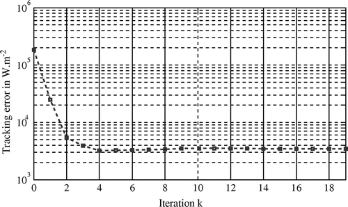
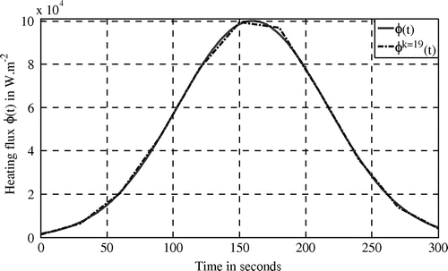
Let the initial value of the flux be defined by ${\overline{\mathit{\varphi }}}^{k=0}(t)=0$. Resolution of inverse problem is performed considering CGM and measured temperature (see continuous line in Figure 3). In Figure 7, tracking error evolution is shown.

Figure 7. Tracking error evolution (Case 1).

According to this minimization, heating flux is accurately identified (see Figure 8 for the identified flux at iteration 19 while cost function is $J({\mathit{\varphi }}^{k=19})\approx 0.69$).

Figure 8. Identified heating flux (Case 1).

At iteration 19, measured temperature $\widehat{\mathit{\theta }}(t)$ and simulated temperature $\mathit{\theta }(C_1,t)$ are quite similar:$$\underset{t\in T}{max}|\widehat{\mathit{\theta }}(t)-\mathit{\theta }(C_1,t)|\approx 0.78\text{K};\underset{t\in T}{max}\left|\frac{\widehat{\mathit{\theta }}(t)-\mathit{\theta }(C_1,t)}{\widehat{\mathit{\theta }}(t)}\right|\approx 0.19\%;$$

The obtained results confirm the CGM algorithm performance in order to identify the strength heating flux $\mathit{\varphi }(t)$. The robustness of this method is highlighted in the following case considering disturbed measurements.

Case 2

Let us consider the same fixed source as in Case 1 but measurements at sensor $C_1$ are disturbed by a Gaussian noise $\mathcal{N}(0,1)$. Then, admissible level of minimization is equal to $J_{stop}=150$ considering the definition proposed in paragraph 3.4. In the following table, both cost function and tracking errors evolutions versus iteration are presented.

Identified and desired (real) heating fluxes are shown in Figure 9.

Figure 9. Identified heating flux (Case 2).

Errors between measured and simulated temperatures (for identified flux at iteration 6) are:$$\underset{t\in T}{max}|\widehat{\mathit{\theta }}(C_1,t)-\mathit{\theta }(C_1,t)|\approx 5\text{K};\underset{t\in T}{max}\left|\frac{\widehat{\mathit{\theta }}(C_1,t)-\mathit{\theta }(C_1,t)}{\widehat{\mathit{\theta }}(C_1,t)}\right|\approx 1.2\%;$$

Considering the previous results, it is shown that convergence of the iterative algorithm is achieved in six iterations and that $J_{stop}$ previously defined is a reliable threshold.

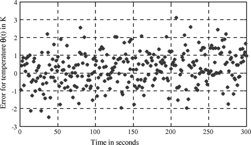
Agreement between measured and predicted temperature (according to the heating flux identified at iteration 6) is shown in Figure 10.

Figure 10. Residual temperature error (Case 2).

Average error is about −0.49 K. It is important to notice that standard deviation between measured and simulated temperature is 1.13 K of the same order of magnitude as Gaussian measurement noise $\mathcal{N}(0,1)$. Thus, even with noisy measurements, identification can be achieved with CGM implementation.

4.2. Mobile heating source

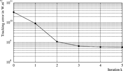
Case 3

Considering the initial heating flux value defined by ${\overline{\mathit{\varphi }}}^{k=0}(t)=0$, resolution of the inverse problem is performed considering CGM and measured temperature (see temperature evolution for sensor $C_1$ in Figure 5). In Figure 11, tracking error evolution is shown.

Figure 11. Tracking error evolution (Case 3).

Identified heating flux is shown in Figure 12. Average relative error is about 0.53%. Measured temperature $\widehat{\mathit{\theta }}(C_1,t)$ and simulated temperature $\mathit{\theta }(C_1,t)$ are quite similar:$$\underset{t\in T}{max}|\widehat{\mathit{\theta }}(C_1,t)-\mathit{\theta }(C_1,t)|\approx 0.11\text{K};\underset{t\in T}{max}\left|\frac{\widehat{\mathit{\theta }}(C_1,t)-\mathit{\theta }(C_1,t)}{\widehat{\mathit{\theta }}(C_1,t)}\right|\approx 0.038\%;$$

Figure 12. Identified heating flux (Case 3).

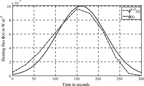
The obtained convergence confirms the efficiency of the conjugate gradient method for the identification of a mobile source strength considering temperature measurements given by a single sensor located on the centre of the upper face (circular trajectory of the heating source is performed on the lower face). In order to validate the robustness of the proposed method, the same objective with a noisy disturbed thermogram is investigated in the following case.

Case 4

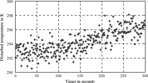
For this final case, let us consider an observed temperature disturbed according to an additive Gaussian noise $\mathcal{N}(0,1)$ (see Figure 13). Such noise is more important considering temperature evolution (Figure 13) than in previous case 2 where maximum temperature is greater than 416 K on the upper plate face (Figure 3).

Figure 13. Disturbed measurements at $C_1$ (Case 4).

Iterative procedure is halted on $J_{stop}=150$ (see paragraph 3.4.) and cost function evolution versus iteration is presented in Table 3.

Table 3. Cost function values at each iteration (Case 4).

Iteration k	0	1	2	3
$J({\mathit{\varphi }}^k)$	625	170	143.8	131.9
Err	$3.34{10}^{10}$	$8.97{10}^9$	8.71 × 10^8	$9.99{10}^8$

The previous numerical results illustrate the role of the admissible level of minimization. Iterative procedure is stopped at $k=2$ (considering Table 3) in order to prevent the convergence of the simulated temperature values (based on the heating flux value) towards the disturbed measured temperature. If iterative procedure is not stopped, heating flux is not well identified (tracking error increases; see Table 3).

Desired and identified heating fluxes are drawn in Figure 14.

Figure 14. Heating flux identification (Case 4).

Errors values between simulated and measured temperatures are:$$\underset{t\in T}{max}|\widehat{\mathit{\theta }}(C_1,t)-\mathit{\theta }(C_1,t)|=3.1\text{K};\underset{t\in T}{max}\left|\frac{\widehat{\mathit{\theta }}(C_1,t)-\mathit{\theta }(C_1,t)}{\widehat{\mathit{\theta }}(C_1,t)}\right|\approx 1\%.$$

Considering the previous values, it is shown that convergence of the iterative algorithm in case 4 is achieved in one iteration. In previous case 2, $J_{stop}=150$ has been obtained at iteration 6. This faster convergence in case 4 is due to the lower level of observed temperature inducing lower values of cost function $J$ (see Tables 2 and 3 for comparison). Agreement between measured and predicted temperature (according to the heating flux identified at iteration 3) is shown in Figure 15.

Figure 15. Residual temperature error (Case 4).

Average residual error of temperature is about 0.24 K. Moreover, standard deviation between measured and simulated temperature is 0.95 K and of the same order of magnitude as Gaussian measurement noise $\mathcal{N}(0,1)$. Thus, even with noisy measurements, identification can be achieved thanks to the CGM implementation.

It is quite important to notice that even if minimization algorithm is stopped after one iteration, identification of unknown heating flux (11 parameters) is performed (see Figure 14). Important noises (see Figure 13 for disturbed observations) lead to an average relative error on identified heating flux equal to 71.3%.

5. Experimental results

The experimental device developed in our research institute is made up three main elements:

• heating source: halogen lamp associated with an optical Kohler device in order to provide a uniform circular heat flux on the lower surface of a metallic plate,

• a micrometric device used to move the heating disc in XZ plane,

• infrared observations on the upper surface of the sample in order to obtain relative temperature measurements for several points.

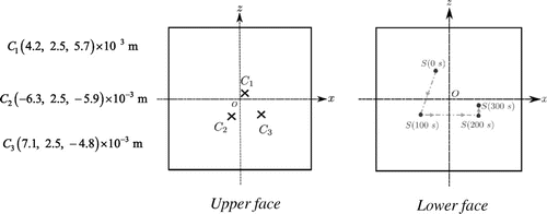
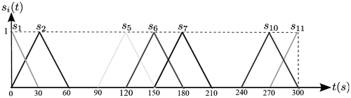
In the following, sample is a square black coated titanium sample (length is 10 cm, thickness is 5 mm). Plate surface centres coordinates are $(0,2.5\times {10}^{-3},0)\text{m}$ and $(0,-2.5\times {10}^{-3},0)\text{m}$. Sensors on the upper face are located at: $(4.2,2.5,5.7)\times {10}^{-3}\text{m}$; $(-6.3,2.5,-5.9)\times {10}^{-3}\text{m}$ and $(7.1,2.5,-4.8)\times {10}^{-3}\text{m}$. Heating source radius is 3 mm and mobile trajectory on the lower surface is described by a piecewise continuous linear function defined in the Table 4 and Figure 16.

Table 4. Mobile source trajectory.

Time (s)	0	100	200	300
$X$ in m	−0.01	−0.02	0.02	0.02
$Z$ in m	0.02	−0.01	−0.01	−0.005

Table 5. Cost function values for several iterations (experimentation).

Iteration k	0	1	2	3	4	5	…	15	…	29	30	…	36
$J({\mathit{\varphi }}^k)$	8694	190	45	41	34	33	…	30	…	29.8	29.7	…	29.6

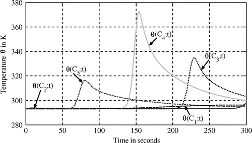
Figure 16. Sensors positions (upper face) and heating source trajectory (lower face).

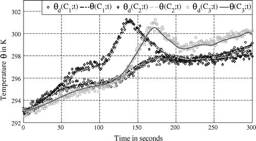
Measured temperatures obtained during 300s are presented Figure 17 (square). Considering the experimental observations presented in Figure 17, the previous identification method has been implemented in order to identify the unknown heating flux every 10 s (31 unknown values have to be determined). Cost function evolution is shown in the following table:

Figure 17. Measured (square) and calculated temperature.

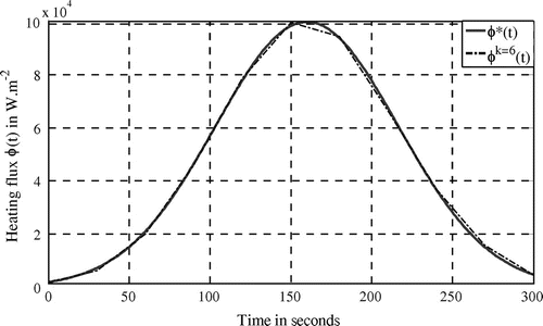
Identified flux at iteration 36 is presented Figure 18.

Figure 18. Identified experimental heating flux.

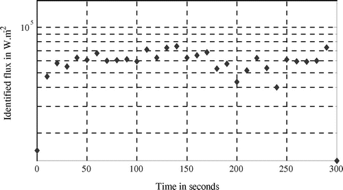
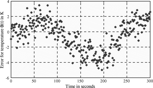
It is shown that the flux is quasi-constant (average value is about $57k\text{W}{\text{m}}^{-2}$). Such result is in adequacy with the experimentation. Moreover, considering residual temperatures (issued from Figure 17) drawn in Figure 19, it is shown that heat flux identification has been accurately performed (see Table 6).

Figure 19. Residual temperature (experimentation).

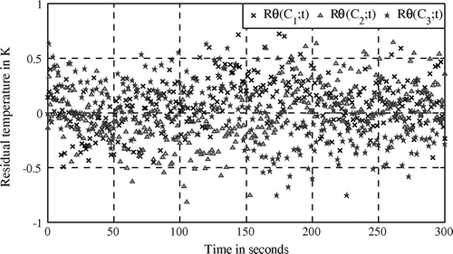
Table 6. Residual temperatures (experimentation).

	Sensor $C_1$	Sensor $C_2$	Sensor $C_3$
Average value	0.08	−0.01	−0.01
Standard deviation	0.23	0.26	0.26

6. Conclusion

In this communication, the identification of the time dependent heating flux generated by a fixed or a mobile source has been investigated in a three-dimensional geometry. The Alifanov’s iterative regularization method has been successfully implemented for such an ill-posed problem (conjugate gradient method with an adjoint equation in order to compute the gradient). At each iteration, conjugate descent directions are computed considering an adjoint problem (issued from Lagrangian formulation) while descent depth is obtained from sensitivity problem resolution (derived from variational calculus). Considering noisy measurements, iterative regularization is reliable and it is shown that minimization algorithm is quite robust. Moreover, convergence is quickly achieved.

Several outlooks can be considered for further works. The simultaneous identification of both trajectory and heat strength of the mobile source can be investigated considering sliding time intervals. Moreover, in many thermal processes, thermal properties of the studied materials are temperature dependent and such nonlinearities have to be carefully taken into account. The last but not the least, an experimental apparatus is actually developed in the LISA research institute in order to test numerous situations with a set of mobile sensors for mobile source tracking.

References

- Muniz WB, de Campos Velho HFD, Ramos FM. A comparison of some inverse methods for estimating the initial condition of the heat equation. J. Comput. Appl. Math. 1999;103:145–163.10.1016/S0377-0427(98)00249-0
- Li HY, Yan WM. Identification of wall heat flux for turbulent forced convection by inverse analysis. Int. J. Heat Mass Transfer. 2003;46:1041–1048.10.1016/S0017-9310(02)00364-2
- Telejko T, Malinowski Z. Application of an inverse solution to the thermal conductivity identification using the finite element method. J. Mater. Process. Technol. 2004;146:145–155.10.1016/j.jmatprotec.2003.10.006
- Silva SMMLE, Vilarinho L, Scotti A, Ong TH, Guimaraes G. Heat flux determination in the gas-tungsten-arc welding process by using a three-dimensional model in inverse heat conduction problem. High Temp. High Press. 2003;35/36:117–126.
- Wippo V, Devrient M, Kern M, Jaeschke P, Frick T, Stute U, Schmidt M, Haferkamp H. Evaluation of a pyrometric-based temperature measuring process for the laser transmission welding. Phys. Procedia. 2012;39:128–136.10.1016/j.phpro.2012.10.022
- Zhou JH, Zhang YW, Chen JK, Feng ZC. Inverse estimation of surface heating condition in a three-dimensional object using conjugate gradient method. Int. J. Heat Mass Transfer. 2010;53:2643–2654.10.1016/j.ijheatmasstransfer.2010.02.048
- Museux N, Perez L, Autrique L, Agay D. Skin burns after laser exposure: histological analysis and predictive simulation. Burns. 2012;38:658–667.10.1016/j.burns.2011.12.006
- Neto AJ, Özişik MN. Simultaneous estimation of location and timewise-varying strength of a plane heat source. Numer. Heat Transfer, Part A. 1993;24:467–477.10.1080/10407789308902635
- Khachfe RA, Jarny Y. Numerical solution of 2-D nonlinear inverse heat conduction problems using finite-element techniques. Numer. Heat Transfer, Part B. 2000;37:45–67.
- Abou khachfe RA, Jarny Y. Determination of heat sources and heat transfer coefficient for two-dimensional heat flow – numerical and experimental study. Int. J. Heat Mass Transfer. 2001;44:1309–1322.10.1016/S0017-9310(00)00186-1
- Lefèvre F, Le Niliot C. Multiple transient point heat sources identification in heat diffusion: application to experimental 2D problems. Int. J. Heat Mass Transfer. 2002;45:1951–1964.10.1016/S0017-9310(01)00299-X
- Beck JV, Blackwell B, Clair CRS. Inverse heat conduction. New York (NY): John Wiley; 1985.
- Hensel E. Inverse theory and applications for engineers. Englewood Cliffs (NJ): Prentice-Hall; 1991.
- Alifanov OM. Inverse heat transfer problems. Berlin: Springer-Verlag; 1979. p. 384.
- Blanc G, Raynaud M, Chau TH. A guide for the use of the function specification method for 2D inverse heat conduction problems. Revue Générale de Thermique. 1998;37:17–30.10.1016/S0035-3159(97)82463-4
- Jarny Y, Ozisik MN, Bardon JP. A general optimization method using adjoint equation for solving multidimensional inverse heat conduction. Int. J. Heat Mass Transfer. 1991;34:2911–2919.10.1016/0017-9310(91)90251-9
- Huang CH, Wang SP. A three-dimensional inverse heat conduction problem in estimating surface heat flux by conjugate gradient method. Int. J. Heat Mass Transfer. 1999;42:3387–3403.10.1016/S0017-9310(99)00020-4
- Huang CH, Chen WC. A three-dimensional inverse forced convection problem in estimating surface heat flux by conjugate gradient method. Int. J. Heat Mass Transfer. 2000;43:3171–3181.10.1016/S0017-9310(99)00330-0
- Rouquette S, Autrique L, Chaussavoine C, Thomas L. Identification of influence factors in a thermal model of a plasma-assisted chemical vapor deposition process. Inverse Prob. Sci. Eng. 2007;15:489–515.10.1080/17415970600838764
- Feng ZC, Chen JK, Zhang YW, Griggs JL. Estimation of front surface temperature and heat flux of a locally heated plate from distributed sensor data on the back surface. Int. J. Heat Mass Transfer. 2011;54:3431–3439.10.1016/j.ijheatmasstransfer.2011.03.043
- Zhou JH, Zhang YW, Chen JK, Feng ZC. Inverse estimation of surface temperature induced by a moving heat source in a 3-D object based on back surface temperature with random measurement errors. Numer. Heat Transfer, Part A. 2012;61:85–100.10.1080/10407782.2012.644166
- Zhou JH, Zhang YW, Chen JK, Feng ZC. Inverse estimation of front surface temperature of a plate with laser heating and convection–radiation cooling. Int. J. Therm. Sci. 2012;52:22–30.10.1016/j.ijthermalsci.2011.09.009
- Dennis B, Dulikravich GS. Inverse determination of unsteady temperatures and heat fluxes on inaccessible boundaries. J. Inverse and III-posed Prob. 2012;20:791–803.
- Gardarein JL, Corre Y, Rigollet F, Le Niliot C, Reichle R, Andrew P. Thermal quadrupoles approach for two-dimensional heat flux estimation using infrared and thermocouple measurements on the JET tokamak. Int. J. Therm. Sci. 2009;48:1–13.10.1016/j.ijthermalsci.2008.02.005
- Gaspar J, Gardarein JL, Rigollet F, Le Niliot C, Corre Y, Devaux S. Nonlinear heat flux estimation in the JET divertor with the ITER like wall. Int. J. Therm. Sci. 2013;72:82–91.10.1016/j.ijthermalsci.2013.04.029
- Le Niliot C, Lefèvre F. A parameter estimation approach to solve the inverse problem of point heat sources identification. Int. J. Heat Mass Transfer. 2004;47:827–841.10.1016/j.ijheatmasstransfer.2003.08.011
- Tarantola A. Inverse problem theory and Methods for Model Parameter Estimation. SIAM Soc. Ind. Appl. Math. 2005:342.
- Perez L, Gillet M, Autrique L. Parametric identification of a multi-layered intumescent system. In: 5th International Conference: Inverse Problems (Identification, Design and Control); 2007 May 10–17; Russia, Moscow.
- Weinstock RP. Calculus of variations. New York (NY): McGraw-Hill; 1952. p. 326.
- Alifanov OM, Artyukhin EA, Rumyantsev SV. Extreme methods for solving ill posed problems with applications to inverse heat transfer problems. New York (NY): Begell House; 1995.
- Powell MJD. Restart procedures for the conjugate gradient method. Math. Program. (North-Holland Publishing Company). 1977;12:241–254.