Estimation of parameter functions in ordinary differential equations with a stage structure: a linear case

Abstract

In many mathematical models with complex parameter functions, it is critical to suggest a strategy for estimating those functions. This paper considers the problem of fitting parameter functions to given data by using a finite number of piecewise functions. Here, the primary aim is to propose several necessary and sufficient conditions that can guarantee the existence of parameter functions. With these criteria, the paper provides an algorithm for solving the parameter estimation problem efficiently. Numerical examples verify that the proposed algorithm is effective in estimating parameter functions in differential equations.

Keywords:

• parameter estimation
• optimization
• distribution of nodes
• inverse problem

AMS Subject Classifications:

• 34A55
• 65D05

1 Introduction

Mathematical modelling using a system of differential equations with a set of parameters has been widely used in most scientific fields, including physics, chemistry, biology, earth and environmental sciences, and engineering. Mathematical problems related with such parameter-dependent differential equations can be classified into forward and inverse problems. Forward problems need the analysis and simulation of the model for given parameter values, whereas inverse problems require the estimation of parameters based on the measurement of output variables. The latter have received considerable attention in the last three decades (see e.g. [1, 2] and the references therein). As statistical approaches to parameter estimation problems, nonlinear regression and other data-fitting methods have been widely used.[3–7]

Among various important problems related to parameter estimation, this paper is particularly interested in the problem of fitting parameter functions to given data by using a finite number of piecewise functions. The primary aim of the paper is to propose some conditions for the existence of parameter functions and introduce an efficient algorithm for estimating these functions. The number of subintervals and the type of basis function in each subinterval are not known a priori, and therefore the main concern is how the number of subintervals and the basis function can be determined and how time nodes can be optimally found for each subinterval.

This paper begins with linear stage-structured differential equations whose parameter functions can be approximated by piecewise constants, and other types of basis functions for approximating parameter functions and nonlinear differential equations with noisy data are left to future research. For a given data-set, the focus is on finding a piecewise constant parameter function in a differential equation to interpolate the data. A necessary and sufficient condition for the existence and uniqueness of the piecewise constant parameter function when subintervals are known is addressed first. In addition, several criteria for determining time nodes and then parameter functions when subintervals are yet to be determined are proposed. These criteria are provided by a $C$-test function in Section 2. An algorithm is suggested to determine time nodes and coefficients for each subinterval optimally with the given data-set and the number of subintervals. Several numerical experiments demonstrate that the algorithm is effective in estimating parameter functions. Further, the solution of the linear stage-structured differential equation with the estimated parameter function provides a good approximation for the solution of the nonlinear differential equation.

The rest of this paper proceeds as follows: Section 2 starts with a formulation of the problem of estimating parameter functions with a linear stage-structured differential equation. A $C$-test function is defined to determine whether there exist suitable solutions of the differential equation to interpolate a set of given data. Section 3 presents the necessary and sufficient conditions for the given data-set to solve the problem of estimating parameter functions when time nodes of subintervals are known. Section 4 derives the conditions by using the $C$-test function for determining parameter functions when time nodes of subintervals are yet to be determined. Section 5 introduces an algorithm for determining parameter functions based on an optimization problem, and Section 6 presents the numerical results for estimated parameter functions and their corresponding solutions based on the proposed algorithm.

2 Parameter estimation problem

2.1 Motivation

Numerous biological phenomena can be described by stage-structured modelling. For instance, growth rates of most fish species are sensitive to seasonal effects, mainly to temperature changes, and it is well known that there is a strong relationship between specific growth rates and temperature for most populations of bacteria (see e.g. [8–10] and the references therein). In addition, many delay differential equations with a stage structure can be found in the literature.[11–15]

For the given data-set ${\{(p_j,q_j)\}}_{j=1}^J,p_1<p_2<\cdots <p_J,$ the following stage-structured differential equation is considered:$$\begin{array}{cc}& \frac{du}{dt}=f(t,u;\mathit{\theta }(t)),t\in (p_1,p_J);\hfill \\ & u(p_j)=q_j\text{for}j=1,\dots ,J.\hfill \end{array}$$with the parameter function1 $$\begin{array}{c}\hfill \mathit{\theta }(t)=\sum _{i=1}^I{\mathit{\theta }}_i{\mathit{\chi }}_{[t_{i-1},t_i)}(t),\end{array}$$1 where the number of intervals $I$, the node $t_i$ and the parameter ${\mathit{\theta }}_i$, $(i=1,\dots ,I)$ are to be determined by assuming that $t_0=p_1.$ Here, $I,t_i$, and ${\mathit{\theta }}_i$ depend on the differential equation and the given data-set ${\{(p_j,q_j)\}}_{j=1}^J$.

2.2 Linear case

This paper focuses on linear stage-structured differential equations by emphasizing the relationship between the parameter function and the data-set. Nonlinear differential equations are left to future research.

Now consider the following estimation problem: For a set of given data ${\{(p_j,q_j)\}}_{j=1}^J,$ find $\mathit{\theta }(t)$ in the form of (11 $$\begin{array}{c}\hfill \mathit{\theta }(t)=\sum _{i=1}^I{\mathit{\theta }}_i{\mathit{\chi }}_{[t_{i-1},t_i)}(t),\end{array}$$1 ) such that2a $$\begin{array}{c}\hfill \frac{du}{dt}=\mathit{\theta }(t)u,t\in (p_1,p_J),\end{array}$$2a 2b $$\begin{array}{c}\hfill u(p_j)=q_j\text{for}j=1,\dots ,J.\end{array}$$2b

Note that the solution $u(t)$ of (2) can be given by3 $$\begin{array}{c}\hfill u(t)=\sum _{i=1}^{I}u(t_{i-1})e^{{\mathit{\theta }}_i(t-t_{i-1})}{\mathit{\chi }}_{[t_{i-1},t_i)}(t),\end{array}$$3 when the parameter function $\mathit{\theta }(t)$ in (11 $$\begin{array}{c}\hfill \mathit{\theta }(t)=\sum _{i=1}^I{\mathit{\theta }}_i{\mathit{\chi }}_{[t_{i-1},t_i)}(t),\end{array}$$1 ) is known.

Because most physical data have positive values, solutions of Equation (2a2a $$\begin{array}{c}\hfill \frac{du}{dt}=\mathit{\theta }(t)u,t\in (p_1,p_J),\end{array}$$2a ) are assumed to be positive and data-sets are restricted to cases such as those described in Definition 2.1.

Definition 2.1

The data-set $D={\{(p_j,q_j)\}}_{j=1}^J$ is called positively well-posed if $D$ has the following two properties:

(i)	${\{p_j\}}_{j=1}^J$ is a strictly increasing sequence,
(ii)	$q_j>0\text{for}j=1,\dots ,J.$

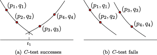
If there is only a single subinterval, then the necessary and sufficient condition for the constant function $\mathit{\theta }$ to be uniquely determined in the interval is summarized in the following lemma:

Lemma 2.2

Suppose that there is a given data set ${\{(p_j,q_j)\}}_{j=1}^J$ that is positively well-posed in a single interval $[t_0,t_1]$. Then the constant function $\mathit{\theta }$ and the solution $u(t)$ satisfying (2) can be uniquely determined if and only if$$dim(\mathrm{s}pan\{(1,p_j,log{q}_j)\mid j=1,\dots ,J\})=2.$$

Proof

Suppose that $u(t)$ satisfies$$\begin{array}{cc}\hfill u(t)& =u(t_0)e^{\mathit{\theta }(t-t_0)},\hfill \\ \hfill u(p_j)& =q_j\text{for}j=1,\dots ,J.\hfill \end{array}$$Then the given data-set ${\{(p_j,q_j)\}}_{j=1}^J$ must satisfy$$log{q}_j=logu(t_0)+\mathit{\theta }(p_j-t_0).$$That is, ${\{(p_j,log{q}_j)\}}_{j=1}^J$ are collinear. The existence and uniqueness of $u(t_0)$ and $\mathit{\theta }$ are equivalent to$$\begin{array}{c}\hfill dim(\mathrm{s}pan\{(1,p_j,log{q}_j)\mid j=1,\dots ,J\})=2.\square \end{array}$$

Before describing the relationship between data points, the $C$-test function is first defined.

Definition 2.3

Define the $C$-test function $C:{(\mathbb{R}\times {\mathbb{R}}_{+})}^3\to \mathbb{R}$ by$$\begin{array}{c}\hfill C(x_1,y_1,x_2,y_2,x_3,y_3):=(x_1-x_2)log{y}_3+(x_2-x_3)log{y}_1+(x_3-x_1)log{y}_2.\end{array}$$

Proposition 2.4

Suppose that $x_1<x_2<x_3$. If the $C$-test function C is positive (or negative), then there exists a log-concave (or log-convex) function that passes through $(x_1,y_1)$, $(x_2,y_2)$ and $(x_3,y_3)$. In addition, the following properties hold:4 $$\begin{array}{cc}& C(x_1,y_1,x_2,y_2,x_3,y_3)\hfill \\ & =-C(x_1,y_1,x_3,y_3,x_2,y_2)\hfill \\ & =C(x_2,y_2,x_3,y_3,x_1,y_1)=-C(x_2,y_2,x_1,y_1,x_3,y_3)\hfill \\ & =C(x_3,y_3,x_1,y_1,x_2,y_2)=-C(x_3,y_3,x_2,y_2,x_1,y_1).\hfill \end{array}$$4

Proof

Note that the $C$-test function $C$ can be rewritten as$$\begin{array}{c}\hfill C(x_1,y_1,x_2,y_2,x_3,y_3)=(x_1-x_2)(x_2-x_3)[\frac{log{y}_1-log{y}_2}{x_1-x_2}-\frac{log{y}_2-log{y}_3}{x_2-x_3}].\end{array}$$Suppose that $C(x_1,y_1,x_2,y_2,x_3,y_3)>0$. Then $(log{y}_1-log{y}_2)/(x_1-x_2)>(log{y}_2-log{y}_3)/(x_2-x_3)$ which implies the existence of a concave quadratic function that passes through $(x_1,log{y}_1),(x_2,log{y}_2)$ and $(x_3,log{y}_3).$ The case of $C(x_1,y_1,x_2,y_2,x_3,y_3)<0$ is similar. Equation (44 $$\begin{array}{cc}& C(x_1,y_1,x_2,y_2,x_3,y_3)\hfill \\ & =-C(x_1,y_1,x_3,y_3,x_2,y_2)\hfill \\ & =C(x_2,y_2,x_3,y_3,x_1,y_1)=-C(x_2,y_2,x_1,y_1,x_3,y_3)\hfill \\ & =C(x_3,y_3,x_1,y_1,x_2,y_2)=-C(x_3,y_3,x_2,y_2,x_1,y_1).\hfill \end{array}$$4 ) follows immediately from the definition of the $C$-test function $C$. $\square$

Remark 2.5

$C(x_1,y_1,x_2,y_2,x_3,y_3)=0$ implies that $(x_1,y_1),(x_2,y_2)$ and $(x_3,y_3)$ lie on one exponential curve: $y=a{e}^{\mathit{\theta }x},$ where$$a=y_j{\left(\frac{y_j}{y_k}\right)}^{\frac{x_j}{x_k-x_j}},\mathit{\theta }=\frac{log{y}_k-log{y}_j}{x_k-x_j},j,k=1,2,3,j\ne k.$$Equivalently, the exponential curve can be rewritten as$$y=y_j{\left(\frac{y_k}{y_j}\right)}^{\frac{x-x_j}{x_k-x_j}},j,k=1,2,3,j\ne k.$$

Definition 2.6

The data-set $D={\{(p_j,q_j)\}}_{j=1}^J$ is called reducible for the parameter estimation problem if and only if there exist three adjacent data points $\{(p_j,q_j),(p_{j+1},q_{j+1}),(p_{j+2},q_{j+2})\},$$(j=1,\dots ,J-2)$ such that $C(p_j,q_j,p_{j+1},q_{j+1},p_{j+2},$$q_{j+2})=0.$ Otherwise, the set of data $D={\{(p_j,q_j)\}}_{j=1}^J$ is called irreducible.

Remark 2.7

Suppose that the given data-set ${\{(p_j,q_j)\}}_{j=1}^J$ is positively well-posed and irreducible in the interval $[t_0,t_I]$ with the partition ${\cup }_{i=1}^I[t_{i-1},t_i)$. Then every subinterval contains no more than two data points if the data-set determines the parameter function $\mathit{\theta }(t)$ to be uniquely fulfilling (2).

3 The case of known subintervals

This section starts by looking at the case in which $t_i,$ ($i=1,\dots ,I$), are given. The following theorem provides the conditions for the given data-set to guarantee the existence and uniqueness of the parameter function $\mathit{\theta }(t)$ and the corresponding solution $u(t)$ of (2).

Theorem 3.1

Let $I=J-1.$ Suppose that the given data set ${\{(p_j,q_j)\}}_{j=1}^J$ is positively well-posed and let $t_0<t_1<\cdots <t_I$ be given time nodes of $[t_0,t_I].$ Then there exists a unique parameter function $\mathit{\theta }(t)$ and its solution $u(t)$ that satisfy (2) if and only if the following condition holds:

If any interval $[t_{k-1},t_k)$ contains two data points, then $k-1$ data points are located in $[t_0,t_{k-1})$ for any $k\in \{1,\dots ,I\}$.

Proof

Rearrange data points as follows:

(i)	For $1\le i\le I$, let $m_i$ be the number of data points in the interval $[t_{i-1},t_i)$ so that $m_1+\cdots +m_I=J$ and $m_i\in \{0,1,2\}$,
(ii)	For $1\le i\le I$, denote ${\{(p_j^i,q_j^i)\}}_{j=1}^{m_i}$ by the set of data points in the interval $[t_{i-1},t_i)$,
(iii)	For $1\le i\le I$, ${\{p_j^i\}}_{j=1}^{m_i}$ is a strictly increasing sequence.

Suppose that there is a continuous function $u(t)$ satisfying$$\begin{array}{c}\hfill \left\{\begin{array}{c}u(t)={\sum }_{i=1}^I\left[u,(t_{i-1}),e^{{\mathit{\theta }}_i(t-t_{i-1})}\right]{\mathit{\chi }}_{[t_{i-1},t_i)}(t).\hfill \\ u(p_j^i)=q_j^{i}j=1,\dots ,m_i,i=1,\dots ,I.\hfill \end{array}\right.\end{array}$$Then the given data $(p_j^i,q_j^i)$ must satisfy5 $$\begin{array}{c}\hfill log{q}_j^i=logu(t_{i-1})+{\mathit{\theta }}_i(p_j^i-t_{i-1})\text{for}1\le j\le m_i,1\le i\le I.\end{array}$$5 And by the continuity conditions, we obtain6 $$\begin{array}{c}\hfill logu(t_i)=logu(t_{i-1})+{\mathit{\theta }}_i(t_i-t_{i-1})\text{for}1\le i\le I-1.\end{array}$$6 Set$$\begin{array}{cc}\hfill \mathbf{x}& ={\left(log,u,(t_0),,,{\mathit{\theta }}_1,,,log,u,(t_1),,,{\mathit{\theta }}_2,,,\dots ,,,log,u,(t_{I-1}),,,{\mathit{\theta }}_I\right)}^t\in {\mathbb{R}}^{2I},\hfill \\ \hfill \mathbf{b}& ={\left(log,q_1^1,,,\dots ,,,log,q_{m_1}^1,,,0,,,log,q_1^2,,,\dots ,,,log,q_{m_2}^2,,,0,,,\dots ,,,0,,,log,q_1^I,,,\dots ,,,log,q_{m_I}^I\right)}^t\in {\mathbb{R}}^{J+I-1}.\hfill \end{array}$$ Combining (55 $$\begin{array}{c}\hfill log{q}_j^i=logu(t_{i-1})+{\mathit{\theta }}_i(p_j^i-t_{i-1})\text{for}1\le j\le m_i,1\le i\le I.\end{array}$$5 ) and (66 $$\begin{array}{c}\hfill logu(t_i)=logu(t_{i-1})+{\mathit{\theta }}_i(t_i-t_{i-1})\text{for}1\le i\le I-1.\end{array}$$6 ), we have$$\mathbf{A}\mathbf{x}=\mathbf{b},$$where the $(J+I-1)\times 2I$ matrix $\mathbf{A}$ is explicitly given by$$\begin{array}{c}\hfill \mathbf{A}=\left[\begin{array}{cccccccccc}1& (p_1^1-t_0)& 0& 0& 0& \cdots & 0& 0& 0& 0\\ ⋮& ⋮& ⋮& ⋮& ⋮& \ddots & ⋮& ⋮& ⋮& ⋮\\ 1& (p_{m_1}^1-t_0)& 0& 0& 0& \cdots & 0& 0& 0& 0\\ 1& (t_1-t_0)& -1& 0& 0& \cdots & 0& 0& 0& 0\\ 0& 0& 1& (p_1^2-t_1)& 0& \cdots & 0& 0& 0& 0\\ ⋮& ⋮& ⋮& ⋮& ⋮& \ddots & ⋮& ⋮& ⋮& ⋮\\ 0& 0& 1& (p_{m_2}^2-t_1)& 0& \cdots & 0& 0& 0& 0\\ 0& 0& 1& (t_2-t_1)& -1& \cdots & 0& 0& 0& 0\\ ⋮& ⋮& ⋮& ⋮& ⋮& \ddots & ⋮& ⋮& ⋮& ⋮\\ 0& 0& 0& 0& 0& \cdots & 1& (p^{I-1}-t_{I-1})& 0& 0\\ ⋮& ⋮& ⋮& ⋮& ⋮& \ddots & ⋮& ⋮& ⋮& ⋮\\ 0& 0& 0& 0& 0& \cdots & 1& (p^{I-1}-t_{I-1})& 0& 0\\ 0& 0& 0& 0& 0& \cdots & 1& (t_I-t_{I-1})& -1& 0\\ 0& 0& 0& 0& 0& \cdots & 0& 0& 1& (p_1^I-t_{I-1})\\ ⋮& ⋮& ⋮& ⋮& ⋮& \ddots & ⋮& ⋮& ⋮& ⋮\\ 0& 0& 0& 0& 0& \cdots & 0& 0& 1& (p_{m_I}^I-t_{I-1})\end{array}\right].\end{array}$$It then follows that the existence of a unique parameter function $\mathit{\theta }(t)$ and the corresponding function $u(t)$ that satisfy (2) is equivalent to the invertibility of the matrix $\mathbf{A}.$ Because $m_i\le 2$ ($i=1,\dots ,I$) and $I=J-1$, there exists at least one $k\in \{1,\dots ,I\}$ such that $m_k=2$ by the pigeon hole principle.

With some elementary operations, $\mathbf{A}$ can be transformed into the following matrix$$\mathbf{A}\sim \left[\begin{array}{ccc}{\mathbf{A}}_1& \mathbf{0}& \mathbf{0}\\ \mathbf{0}& {\mathbf{A}}_2& \mathbf{0}\\ \mathbf{0}& \mathbf{0}& {\mathbf{A}}_3\end{array}\right],$$where $\mathbf{0}$ denotes a zero block matrix and$${\mathbf{A}}_1=\left[\begin{array}{cccccc}1& (p_1^1-t_0)& 0& \cdots & 0& 0\\ ⋮& ⋮& ⋮& ⋮& ⋮& ⋮\\ 1& (p_{m_1}^1-t_0)& 0& \cdots & 0& 0\\ 1& (t_1-t_0)& -1& \cdots & 0& 0\\ ⋮& ⋮& ⋮& \ddots & ⋮& ⋮\\ 0& 0& 0& \cdots & 1& (p_1^{k-1}-t_{k-2})\\ ⋮& ⋮& ⋮& ⋮& ⋮& ⋮\\ 0& 0& 0& \cdots & 1& (p_{m_{k-1}}^{k-1}-t_{k-2})\\ 0& 0& 0& \cdots & 1& (t_{k-1}-t_{k-2})\end{array}\right],$$$${\mathbf{A}}_2=\left[\begin{array}{cc}1& 0\\ 0& 1\end{array}\right],$$and$${\mathbf{A}}_3=\left[\begin{array}{cccccc}-1& 0& 0& \cdots & 0& 0\\ 1& (p_1^{k+1}-t_k)& 0& \cdots & 0& 0\\ ⋮& ⋮& ⋮& ⋮& ⋮& ⋮\\ 1& (p_{m_{k+1}}^{k+1}-t_k)& 0& \cdots & 0& 0\\ 1& (t_{k+1}-t_k)& -1& \cdots & 0& 0\\ ⋮& ⋮& ⋮& \ddots & ⋮& ⋮\\ 0& 0& 0& \cdots & 1& (p_1^I-t_{I-1})\\ ⋮& ⋮& ⋮& ⋮& ⋮& ⋮\\ 0& 0& 0& \cdots & 1& (p_{m_I}^I-t_{I-1})\end{array}\right].$$Since$$\begin{array}{cc}\hfill \mathrm{r}ank({\mathbf{A}}_1)& \le min\{m_1+\cdots +m_{k-1}+(k-1),2(k-1)\},\hfill \\ \hfill \mathrm{r}ank({\mathbf{A}}_2)& =2,\hfill \\ \hfill \mathrm{r}ank({\mathbf{A}}_3)& \le min\{m_{k+1}+\cdots +m_I+(I-k),2(I-k)\},\hfill \end{array}$$the following can be obtained by recalling $I=J+1={\sum }_{j=1}^I{m}_j+1$ :$$\begin{array}{cc}\hfill \mathrm{r}ank(\mathbf{A})=& \mathrm{r}ank({\mathbf{A}}_1)+\mathrm{r}ank({\mathbf{A}}_2)+\mathrm{r}ank({\mathbf{A}}_3)\hfill \\ \hfill \le & min\{m_1+\cdots +m_{k-1}+(k-1),2(k-1)\}+2\hfill \\ & +min\{m_{k+1}+\cdots +m_I+(I-k),2(I-k)\}\hfill \\ \hfill =& min\{m_1+\cdots +m_{k-1}+(k-1),2(k-1)\}+2\hfill \\ & +min\{(2I-k-1)-(m_1+\cdots +m_{k-1}),2(I-k)\}\hfill \\ \hfill =& min\{m_1+\cdots +m_{k-1},k-1\}+(k-1)+2\hfill \\ & -max\{m_1+\cdots +m_{k-1},k-1\}+(2I-k-1).\hfill \end{array}$$Based on the above, in the case of $m_1+\cdots +m_{k-1}\ne k-1$, $\mathrm{r}ank(\mathbf{A})<2I$, and thus $\mathbf{A}$ is not invertible. Therefore, there is a need for the condition $m_1+\cdots +m_{k-1}=k-1$ with $m_k=2$ to make $\mathbf{A}$ invertible. $\square$

Remark 3.2

   

(i)	Theorem 3.1 provides the necessary and sufficient condition for data and subintervals for the determination of a parameter function $\mathit{\theta }(t)$ uniquely to fulfil (2). That is, if a subinterval contains two data points, then the number of data points should equal that of subintervals in the whole left side of the interval.
(ii)	In the case of $I>J-1,$$\mathrm{r}ank(\mathbf{A})\le J+I-1<2I,$ and therefore $\mathbf{A}$ is not invertible. Although the parameter function $\mathit{\theta }(t)$ can be determined, the uniqueness of $\mathit{\theta }(t)$ and its corresponding function $u(t)$ satisfying (2) cannot be guaranteed.
(iii)	In the case of $I<J-1,$ there is an over-determined problem. The only case in which the over-determined system $\mathbf{A}\mathbf{x}=\mathbf{b}$ has a unique solution is that the linear system can be reduced to the system ${\mathbf{A}}^{\prime }\mathbf{x}={\mathbf{b}}^{\prime }$ with $\mathrm{r}ank({\mathbf{A}}^{\prime })=2I.$

Remark 3.3

Let ${\{(p_j,q_j)\}}_{j=1}^J$ a given data-set that is positively well posed and $t_0<t_1<\cdots <t_I$ be given time nodes in $[t_0,t_I]$ with $I=J-1.$ Suppose that there are two consecutive subintervals $[t_{k-1},t_k)$ and $[t_k,t_{k+1})$ containing two data points in each subinterval. Then the parameter function $\mathit{\theta }(t)$ cannot be determined uniquely. Indeed, for $\mathit{\theta }(t)$ to be determined uniquely, Theorem 3.1 requires that $[t_0,t_{k-1})$ and $[t_0,t_k)$ contain $k-1$ and $k$ data points, respectively, which leads to a contradiction.

4 The case of subintervals not yet determined

The previous section describes the necessary and sufficient condition for a data-set to determine a parameter function and its corresponding solution uniquely when $I=J-1.$ The parameter function estimation problem is over-determined in the case of $I<J-1.$ If the problem is over-determined with too much information, then a particular solution may not exist. As one way to address this problem, the number of unknown parameters can be increased by assuming that time nodes ${\{t_i\}}_{i=1}^{I-1}$ need to be determined. Suppose a given data-set ${\{(p_j,q_j)\}}_{j=1}^J$ is positively well-posed and irreducible. Then every subinterval should have at most two data points. Note that in each subinterval, the constant value of the parameter $\mathit{\theta }$ and its corresponding solution $u(t)$ is uniquely determined by two data points. Therefore, to determine the parameter function for the whole interval, the following types of contiguous subintervals need to be considered:

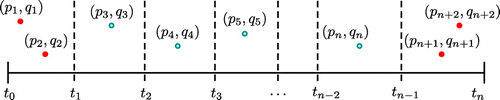
(T1)	The first and last subintervals in this category both contain two data points, whereas all other subintervals contain only one data point,
(T2)	Only the first or last subinterval in this category contains two data points, whereas all other subintervals contain only one data point.

In the case of T2, the existence of $t_i$ and the corresponding parameter ${\mathit{\theta }}_i$ is always guaranteed, and therefore this section focuses on the case of T1. Note that $I=J-2$ in the case of T1.

Figure 1. For given data with $I=2,$$t_1$ can be uniquely determined in case (a), whereas $t_1$ cannot be determined in case (b).

Lemma 4.1

Assume that $x_1,x_2$ and $x_3$ are any nonzero real numbers. Then the following two conditions are equivalent:

(i)	$x_1·x_3<0$ or $x_2·x_3>0$,
(ii)	$x_1·x_2>0$ or $x_2·x_3>0.$

Proof

Suppose (ii) is not true, that is, $x_1·x_2<0\text{and}{x}_2·x_3<0.$ Then $x_1·x_3>0\text{and}{x}_2·x_3>0,$ which implies that (i) is not true. By contrapositive, this completes the proof. $\square$

Lemma 4.2

Suppose that $I=2$ and the given data set ${\{(p_j,q_j)\}}_{j=1}^4$ is positively well-posed and irreducible over the whole interval $[t_0,t_2].$ Then there exist unique $t_1\in [p_2,p_3]$ and the corresponding parameters ${\mathit{\theta }}_1$ and ${\mathit{\theta }}_2$ such that the function $u(t)$ given by (33 $$\begin{array}{c}\hfill u(t)=\sum _{i=1}^{I}u(t_{i-1})e^{{\mathit{\theta }}_i(t-t_{i-1})}{\mathit{\chi }}_{[t_{i-1},t_i)}(t),\end{array}$$3 ) satisfies (2) if and only if$$C(p_1,q_1,p_2,q_2,p_3,q_3)\times C(p_2,q_2,p_3,q_3,p_4,q_4)\ge 0.$$

Proof

Suppose that there exist $t_1\in [p_2,p_3]$ and the corresponding parameters ${\mathit{\theta }}_1$ and ${\mathit{\theta }}_2$ such that the function $u(t)$ given by (33 $$\begin{array}{c}\hfill u(t)=\sum _{i=1}^{I}u(t_{i-1})e^{{\mathit{\theta }}_i(t-t_{i-1})}{\mathit{\chi }}_{[t_{i-1},t_i)}(t),\end{array}$$3 ) satisfies (2). Then we have$$\begin{array}{c}\hfill u(t)=u(t_0)e^{{\mathit{\theta }}_1(t-t_0)}{\mathit{\chi }}_{[t_0,t_1)}(t)+u(t_1)e^{{\mathit{\theta }}_2(t-t_1)}{\mathit{\chi }}_{[t_1,t_2)}(t)\in C^0(t_0,t_2),\end{array}$$and (2b2b $$\begin{array}{c}\hfill u(p_j)=q_j\text{for}j=1,\dots ,J.\end{array}$$2b ) also requires the following relationships:$$\begin{array}{cc}\hfill u(t_0)e^{{\mathit{\theta }}_1(p_1-t_0)}=q_1,& u(t_0)e^{{\mathit{\theta }}_1(p_2-t_0)}=q_2,\hfill \\ \hfill u(t_1)e^{{\mathit{\theta }}_2(p_3-t_1)}=q_3,& u(t_1)e^{{\mathit{\theta }}_2(p_4-t_1)}=q_4.\hfill \end{array}$$The parameter values of ${\mathit{\theta }}_1$ and ${\mathit{\theta }}_2$ and the logarithmic values of $u(t_0)$ and $u(t_1)$ can be determined in terms of ${\{(p_j,q_j)\}}_{j=1}^4$ by solving the above equations:7 $$\begin{array}{cc}& {\mathit{\theta }}_1=\frac{log{q}_1-log{q}_2}{p_1-p_2},{\mathit{\theta }}_2=\frac{log{q}_3-log{q}_4}{p_3-p_4},\hfill \\ & logu(t_0)=\frac{log{q}_1-log{q}_2}{p_1-p_2}{t}_0+\frac{p_{1}log{q}_2-p_{2}log{q}_1}{p_1-p_2},\hfill \\ & logu(t_1)=\frac{log{q}_3-log{q}_4}{p_3-p_4}{t}_1+\frac{p_{3}log{q}_4-p_{4}log{q}_3}{p_3-p_4}.\hfill \end{array}$$7 From the continuity condition ${lim}_{t\to t_1-}u(t)=u(t_1)$, we have8 $$\begin{array}{c}\hfill u(t_1)=u(t_0)e^{{\mathit{\theta }}_1(t_1-t_0)}.\end{array}$$8 Combining (77 $$\begin{array}{cc}& {\mathit{\theta }}_1=\frac{log{q}_1-log{q}_2}{p_1-p_2},{\mathit{\theta }}_2=\frac{log{q}_3-log{q}_4}{p_3-p_4},\hfill \\ & logu(t_0)=\frac{log{q}_1-log{q}_2}{p_1-p_2}{t}_0+\frac{p_{1}log{q}_2-p_{2}log{q}_1}{p_1-p_2},\hfill \\ & logu(t_1)=\frac{log{q}_3-log{q}_4}{p_3-p_4}{t}_1+\frac{p_{3}log{q}_4-p_{4}log{q}_3}{p_3-p_4}.\hfill \end{array}$$7 ) and (88 $$\begin{array}{c}\hfill u(t_1)=u(t_0)e^{{\mathit{\theta }}_1(t_1-t_0)}.\end{array}$$8 ) gives9 $$\begin{array}{c}\hfill {\displaystyle \frac{log{q}_3-log{q}_4}{p_3-p_4}{t}_1+\frac{p_{3}log{q}_4-p_{4}log{q}_3}{p_3-p_4}=\frac{log{q}_1-log{q}_2}{p_1-p_2}{t}_1+\frac{p_{1}log{q}_2-p_{2}log{q}_1}{p_1-p_2},}\end{array}$$9 and finally,$$\begin{array}{c}\hfill t_1=-\left(\frac{p_{1}log{q}_2-p_{2}log{q}_1}{p_1-p_2},-,\frac{p_{3}log{q}_4-p_{4}log{q}_3}{p_3-p_4}\right)/\left(\frac{log{q}_1-log{q}_2}{p_1-p_2},-,\frac{log{q}_3-log{q}_4}{p_3-p_4}\right).\end{array}$$ Now the condition in which $t_1$ lies between $p_2$ and $p_3$ needs to be derived (see Figure 1). This condition can be restated as $(t_1-p_2)(t_1-p_3)\le 0,$ and a direct calculation gives$$\begin{array}{cc}\hfill 0& \ge (t_1-p_2)(t_1-p_3)\hfill \\ & =-\frac{C(p_1,q_1,p_2,q_2,p_3,q_3)\times C(p_2,q_2,p_3,q_3,p_4,q_4)}{(p_1-p_2)(p_3-p_4)(\frac{log{q}_1-log{q}_2}{p_1-p_2}-\frac{log{q}_3-log{q}_4}{p_3-p_4}{)}^2}.\hfill \end{array}$$Note that the denominator is not zero because data points are irreducible. Therefore, $t_1\in [p_2,p_3]$ if and only if $C(p_1,q_1,p_2,q_2,p_3,q_3)\times C(p_2,q_2,p_3,q_3,p_4,q_4)\ge 0.$$\square$

Lemma 4.3

Suppose that $I=3$ and the given data set ${\{(p_j,q_j)\}}_{j=1}^5$ is positively well-posed and irreducible over the whole interval $[t_0,t_3].$ Then there exist $t_1\in [p_2,p_3],$$t_2\in [p_3,p_4]$ and corresponding parameters ${\mathit{\theta }}_1,{\mathit{\theta }}_2,$ and ${\mathit{\theta }}_3$ such that the function $u(t)$ given by (33 $$\begin{array}{c}\hfill u(t)=\sum _{i=1}^{I}u(t_{i-1})e^{{\mathit{\theta }}_i(t-t_{i-1})}{\mathit{\chi }}_{[t_{i-1},t_i)}(t),\end{array}$$3 ) satisfies (2) if and only if$$\begin{array}{cc}& C(p_1,q_1,p_2,q_2,p_3,q_3)\times C(p_2,q_2,p_3,q_3,p_4,q_4)\ge 0\text{or}\hfill \\ & C(p_2,q_2,p_3,q_3,p_4,q_4)\times C(p_3,q_3,p_4,q_4,p_5,q_5)\ge 0.\hfill \end{array}$$

Figure 2. An example of the case in which five data points satisfy the $C$-test condition.

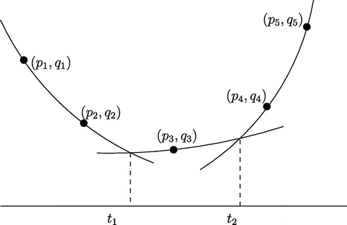
Proof

Suppose that there exist two free nodes $t_1$ and $t_2$ such that following conditions hold (see Figure 2):10 $$\begin{array}{cc}& u(t_0)e^{{\mathit{\theta }}_1(p_1-t_0)}=q_1,u(t_0)e^{{\mathit{\theta }}_1(p_2-t_0)}=q_2,u(t_1)e^{{\mathit{\theta }}_2(p_3-t_1)}=q_3,\hfill \\ & u(t_2)e^{{\mathit{\theta }}_3(p_4-t_2)}=q_4,u(t_2)e^{{\mathit{\theta }}_3(p_5-t_2)}=q_5.\hfill \end{array}$$10 For this problem, we need to determine eight variables ${\mathit{\theta }}_1,{\mathit{\theta }}_2,{\mathit{\theta }}_3,u(t_0),u(t_1),u(t_2),t_1$ and $t_2$. From (1010 $$\begin{array}{cc}& u(t_0)e^{{\mathit{\theta }}_1(p_1-t_0)}=q_1,u(t_0)e^{{\mathit{\theta }}_1(p_2-t_0)}=q_2,u(t_1)e^{{\mathit{\theta }}_2(p_3-t_1)}=q_3,\hfill \\ & u(t_2)e^{{\mathit{\theta }}_3(p_4-t_2)}=q_4,u(t_2)e^{{\mathit{\theta }}_3(p_5-t_2)}=q_5.\hfill \end{array}$$10 ), it is clear that11 $$\begin{array}{cc}& {\displaystyle {\mathit{\theta }}_1=\frac{log{q}_1-log{q}_2}{p_1-p_2},{\mathit{\theta }}_3=\frac{log{q}_4-log{q}_5}{p_4-p_5},}\hfill \\ & {\displaystyle logu(t_0)=\frac{log{q}_1-log{q}_2}{p_1-p_2}{t}_0+\frac{p_{1}log{q}_2-p_{2}log{q}_1}{p_1-p_2},}\hfill \\ & {\displaystyle logu(t_2)=\frac{log{q}_4-log{q}_5}{p_4-p_5}{t}_2+\frac{p_{4}log{q}_5-p_{5}log{q}_4}{p_4-p_5}.}\hfill \end{array}$$11 By the continuity condition of the solution12 $$\begin{array}{cc}& {\displaystyle logu(t_1)=\frac{log{q}_1-log{q}_2}{p_1-p_2}{t}_1+\frac{p_{1}log{q}_2-p_{2}log{q}_1}{p_1-p_2},}\hfill \\ & {\displaystyle u(t_1)e^{{\mathit{\theta }}_2(t_2-t_1)}=u(t_2).}\hfill \end{array}$$12 Therefore, ${\mathit{\theta }}_1,{\mathit{\theta }}_3,u(t_0),u(t_1)$ and $u(t_2)$ can be determined by $t_1,t_2,{\mathit{\theta }}_2,$ and the data-set ${\{(p_j,q_j)\}}_{j=1}^5$. However, ${\mathit{\theta }}_2$ is related to $t_1$ and $t_2$, and therefore showing the existence of ${\mathit{\theta }}_2$ is equivalent to showing that the algebraic system$$\begin{array}{cc}\hfill log{q}_3-logu(t_1)& ={\mathit{\theta }}_2(p_3-t_1),\hfill \\ \hfill logu(t_2)-logu(t_1)& ={\mathit{\theta }}_2(t_2-t_1)\hfill \end{array}$$has at least one solution ${\mathit{\theta }}_2$. This leads to the relationship$$\begin{array}{c}\hfill {\displaystyle \frac{log{q}_3-logu(t_1)}{p_3-t_1}=\frac{logu(t_2)-logu(t_1)}{t_2-t_1},}\end{array}$$which is equivalent to13 $$\begin{array}{c}\hfill (p_3-t_2)logu(t_1)-(t_1-t_2)log{q}_3+(t_1-p_3)logu(t_2)=0.\end{array}$$13 Combining Equations (1111 $$\begin{array}{cc}& {\displaystyle {\mathit{\theta }}_1=\frac{log{q}_1-log{q}_2}{p_1-p_2},{\mathit{\theta }}_3=\frac{log{q}_4-log{q}_5}{p_4-p_5},}\hfill \\ & {\displaystyle logu(t_0)=\frac{log{q}_1-log{q}_2}{p_1-p_2}{t}_0+\frac{p_{1}log{q}_2-p_{2}log{q}_1}{p_1-p_2},}\hfill \\ & {\displaystyle logu(t_2)=\frac{log{q}_4-log{q}_5}{p_4-p_5}{t}_2+\frac{p_{4}log{q}_5-p_{5}log{q}_4}{p_4-p_5}.}\hfill \end{array}$$11 ), (1212 $$\begin{array}{cc}& {\displaystyle logu(t_1)=\frac{log{q}_1-log{q}_2}{p_1-p_2}{t}_1+\frac{p_{1}log{q}_2-p_{2}log{q}_1}{p_1-p_2},}\hfill \\ & {\displaystyle u(t_1)e^{{\mathit{\theta }}_2(t_2-t_1)}=u(t_2).}\hfill \end{array}$$12 ) and (1313 $$\begin{array}{c}\hfill (p_3-t_2)logu(t_1)-(t_1-t_2)log{q}_3+(t_1-p_3)logu(t_2)=0.\end{array}$$13 ) gives14 $$\begin{array}{cc}\hfill 0=& \left(\frac{log{q}_1-log{q}_2}{p_1-p_2},-,\frac{log{q}_4-log{q}_5}{p_4-p_5}\right)t_1{t}_2\hfill \\ & -\left({\displaystyle \frac{log{q}_1-log{q}_2}{p_1-p_2}{p}_3-log{q}_3+\frac{p_{4}log{q}_5-p_{5}log{q}_4}{p_4-p_5}}\right)t_1\hfill \\ & +\left({\displaystyle \frac{p_{1}log{q}_2-p_{2}log{q}_1}{p_1-p_2}-log{q}_3+\frac{log{q}_4-log{q}_5}{p_4-p_5}{p}_3}\right)t_2\hfill \\ & -\left({\displaystyle \frac{p_{1}log{q}_2-p_{2}log{q}_1}{p_1-p_2}-\frac{p_{4}log{q}_5-p_{5}log{q}_4}{p_4-p_5}}\right)p_3.\hfill \end{array}$$14 The RHS of (1414 $$\begin{array}{cc}\hfill 0=& \left(\frac{log{q}_1-log{q}_2}{p_1-p_2},-,\frac{log{q}_4-log{q}_5}{p_4-p_5}\right)t_1{t}_2\hfill \\ & -\left({\displaystyle \frac{log{q}_1-log{q}_2}{p_1-p_2}{p}_3-log{q}_3+\frac{p_{4}log{q}_5-p_{5}log{q}_4}{p_4-p_5}}\right)t_1\hfill \\ & +\left({\displaystyle \frac{p_{1}log{q}_2-p_{2}log{q}_1}{p_1-p_2}-log{q}_3+\frac{log{q}_4-log{q}_5}{p_4-p_5}{p}_3}\right)t_2\hfill \\ & -\left({\displaystyle \frac{p_{1}log{q}_2-p_{2}log{q}_1}{p_1-p_2}-\frac{p_{4}log{q}_5-p_{5}log{q}_4}{p_4-p_5}}\right)p_3.\hfill \end{array}$$14 ) is denoted as $f(t_1,t_2)$. Then the roots of the function $f$ in the rectangular domain $[p_2,p_3]\times [p_3,p_4]$ are considered. Since $f$ is a polynomial of $t_1,t_2$ and $f(p_3,p_3)=0,$ the function $f(t_1,t_2)$ has roots in the domain $[p_2,p_3]\times [p_3,p_4],$ provided that$$\begin{array}{c}\hfill f(p_2,p_3)\times f(p_2,p_4)\le 0\text{or}f(p_2,p_4)\times f(p_3,p_4)\le 0.\end{array}$$Representing the above conditions by using the $C$-function (see the Appendix) gives$$\begin{array}{cc}& C(p_1,q_1,p_2,q_2,p_3,q_3)\times C(p_2,q_2,p_3,q_3,p_4,q_4)\ge 0\text{or}\hfill \\ & C(p_2,q_2,p_3,q_3,p_4,q_4)\times C(p_3,q_3,p_4,q_4,p_5,q_5)\ge 0,\hfill \end{array}$$which completes the proof. $\square$

Lemma 4.3 can be extended to general cases.

Theorem 4.4

($C$-test)   Suppose that $I=n+2$ ($n$ is a positive integer) and the given data set ${\{(p_j,q_j)\}}_{j=1}^{n+4}$ is positively well-posed and irreducible over the whole interval $[t_0,t_{n+2}].$ Then there exist $t_i\in [p_{i+1},p_{i+2}]$ for all $i=1,\dots ,n+1$, and corresponding parameters ${\mathit{\theta }}_1,\dots ,{\mathit{\theta }}_{n+2}$ such that the function $u(t)$ given by (33 $$\begin{array}{c}\hfill u(t)=\sum _{i=1}^{I}u(t_{i-1})e^{{\mathit{\theta }}_i(t-t_{i-1})}{\mathit{\chi }}_{[t_{i-1},t_i)}(t),\end{array}$$3 ) satisfies (2) if and only if15 $$\begin{array}{c}\hfill C(p_i,q_i,p_{i+1},q_{i+1},p_{i+2},q_{i+2})\times C(p_{i+1},q_{i+1},p_{i+2},q_{i+2},p_{i+3},q_{i+3})\ge 0\end{array}$$15 for some $i\in \{1,\dots ,n+1\}.$

Proof

As in Lemma 4.3, the theorem holds for $n=1$. Assume that it also holds for $n-1$.

($\Rightarrow$)Suppose that there exist $t_i\in [p_{i+1},p_{i+2}]$ for all $i=1,\dots ,n+1$, and corresponding parameters ${\mathit{\theta }}_1,\dots ,{\mathit{\theta }}_{n+2}$ such that the function $u(t)$ given by (33 $$\begin{array}{c}\hfill u(t)=\sum _{i=1}^{I}u(t_{i-1})e^{{\mathit{\theta }}_i(t-t_{i-1})}{\mathit{\chi }}_{[t_{i-1},t_i)}(t),\end{array}$$3 ) satisfies (2). By the continuity condition as in Equation (99 $$\begin{array}{c}\hfill {\displaystyle \frac{log{q}_3-log{q}_4}{p_3-p_4}{t}_1+\frac{p_{3}log{q}_4-p_{4}log{q}_3}{p_3-p_4}=\frac{log{q}_1-log{q}_2}{p_1-p_2}{t}_1+\frac{p_{1}log{q}_2-p_{2}log{q}_1}{p_1-p_2},}\end{array}$$9 ), we have$$\begin{array}{c}\hfill {\displaystyle logu(t_1)=\frac{log{q}_1-log{q}_2}{p_1-p_2}{t}_1+\frac{p_{1}log{q}_2-p_{2}log{q}_1}{p_1-p_2}.}\end{array}$$Now consider the new data-set $\{(t_1,u(t_1))\}\cup {\{(p_j,q_j)\}}_{j=3}^{n+4}.$ Since the theorem holds for $n-1,$ the following condition holds:16 $$\begin{array}{cc}& C(t_1,u(t_1),p_3,q_3,p_4,q_4)\times C(p_3,q_3,p_4,q_4,p_5,q_5)\ge 0\text{or}\hfill \\ & C(p_i,q_i,p_{i+1},q_{i+1},p_{i+2},q_{i+2})\times C(p_{i+1},q_{i+1},p_{i+2},q_{i+2},p_{i+3},q_{i+3})\ge 0\hfill \end{array}$$16 for some $i\in \{3,\dots ,n+1\}$. Define $L:\mathbb{R}\to \mathbb{R}$ by $L(t_1):=C(t_1,u(t_1),p_3,q_3,p_4,q_4),$ that is,$$\begin{array}{cc}\hfill L(t_1)=& (p_3-p_4)logu(t_1)+(p_4-t_1)log{q}_3+(t_1-p_3)log{q}_4\hfill \\ \hfill =& {\displaystyle (p_3-p_4)(\frac{log{q}_1-log{q}_2}{p_1-p_2}{t}_1+\frac{p_{1}log{q}_2-p_{2}log{q}_1}{p_1-p_2})MYAMP]+(p_4-t_1)log{q}_3+(t_1-p_3)log{q}_4.}\hfill \end{array}$$Since $L$ is a linear function of $t_1$ and $p_2\le t_1\le p_3$, the condition (1616 $$\begin{array}{cc}& C(t_1,u(t_1),p_3,q_3,p_4,q_4)\times C(p_3,q_3,p_4,q_4,p_5,q_5)\ge 0\text{or}\hfill \\ & C(p_i,q_i,p_{i+1},q_{i+1},p_{i+2},q_{i+2})\times C(p_{i+1},q_{i+1},p_{i+2},q_{i+2},p_{i+3},q_{i+3})\ge 0\hfill \end{array}$$16 ) implies$$\begin{array}{c}\hfill L(p_2)\times C(p_3,q_3,p_4,q_4,p_5,q_5)\ge 0\text{or}L(p_3)\times C(p_3,q_3,p_4,q_4,p_5,q_5)\ge 0.\end{array}$$From the calculation, we get$$\begin{array}{c}\hfill L(p_2)\times C(p_3,q_3,p_4,q_4,p_5,q_5)=C(p_2,q_2,p_3,q_3,p_4,q_4)\times C(p_3,q_3,p_4,q_4,p_5,q_5)\end{array}$$and$$\begin{array}{cc}& L(p_3)\times C(p_3,q_3,p_4,q_4,p_5,q_5)\hfill \\ & =-\left({\displaystyle \frac{p_3-p_4}{p_1-p_2}}\right)\times C(p_1,q_1,p_2,q_2,p_3,q_3)\times C(p_3,q_3,p_4,q_4,p_5,q_5).\hfill \end{array}$$Therefore,$$\begin{array}{cc}& C(p_2,q_2,p_3,q_3,p_4,q_4)\times C(p_3,q_3,p_4,q_4,p_5,q_5)\ge 0\text{or}\hfill \\ & C(p_1,q_1,p_2,q_2,p_3,q_3)\times C(p_3,q_3,p_4,q_4,p_5,q_5)\le 0.\hfill \end{array}$$By Lemma 4.1, we obtain$$\begin{array}{cc}& C(p_1,q_1,p_2,q_2,p_3,q_3)\times C(p_2,q_2,p_3,q_3,p_4,q_4)\ge 0\text{or}\hfill \\ & C(p_2,q_2,p_3,q_3,p_4,q_4)\times C(p_3,q_3,p_4,q_4,p_5,q_5)\ge 0.\hfill \end{array}$$This means that there exists $i\in \{1,\dots ,n+1\}$ such that (1515 $$\begin{array}{c}\hfill C(p_i,q_i,p_{i+1},q_{i+1},p_{i+2},q_{i+2})\times C(p_{i+1},q_{i+1},p_{i+2},q_{i+2},p_{i+3},q_{i+3})\ge 0\end{array}$$15 ) holds.

($\Leftarrow$)Suppose that (1515 $$\begin{array}{c}\hfill C(p_i,q_i,p_{i+1},q_{i+1},p_{i+2},q_{i+2})\times C(p_{i+1},q_{i+1},p_{i+2},q_{i+2},p_{i+3},q_{i+3})\ge 0\end{array}$$15 ) holds for some $i\in \{1,\dots ,n\}.$ Then consider the new data-set ${\{(p_j,q_j)\}}_{j=1}^{n+3}.$ Since the theorem holds for $n-1,$ there exist $t_i\in [p_{i+1},p_{i+2}]$ for all $i=1,\dots ,n$, and corresponding parameters ${\mathit{\theta }}_1,\dots ,{\mathit{\theta }}_{n+1}$ such that the function $u(t)$ given by (33 $$\begin{array}{c}\hfill u(t)=\sum _{i=1}^{I}u(t_{i-1})e^{{\mathit{\theta }}_i(t-t_{i-1})}{\mathit{\chi }}_{[t_{i-1},t_i)}(t),\end{array}$$3 ) satisfies (2). If $t_{n+1}=p_{n+3}$ is chosen, then ${\mathit{\theta }}_{n+2}$ can be determined such that the function $u(t)$ in the subinterval $[t_{n+1},t_{n+2}]$ passes the data point $(p_{n+4},q_{n+4}).$ Suppose that (1515 $$\begin{array}{c}\hfill C(p_i,q_i,p_{i+1},q_{i+1},p_{i+2},q_{i+2})\times C(p_{i+1},q_{i+1},p_{i+2},q_{i+2},p_{i+3},q_{i+3})\ge 0\end{array}$$15 ) holds for some $i=n+1.$ Then consider the new data-set ${\{(p_j,q_j)\}}_{j=2}^{n+4}.$ By similar arguments, $t_i\in [p_{i+1},p_{i+2}]$ can be constructed for all $i=1,\dots ,n+1$, and corresponding parameters ${\mathit{\theta }}_1,\dots ,{\mathit{\theta }}_{n+2}.$$\square$

Figure 3. The first and last intervals both contain two data points, whereas the others, only one data point (T1).

Remark 4.5

Under the assumption of the irreducibility of data points, the value of the $C$-function is always nonzero. From this fact, the condition (1515 $$\begin{array}{c}\hfill C(p_i,q_i,p_{i+1},q_{i+1},p_{i+2},q_{i+2})\times C(p_{i+1},q_{i+1},p_{i+2},q_{i+2},p_{i+3},q_{i+3})\ge 0\end{array}$$15 ) can be rewritten as (1717 $$\begin{array}{c}\hfill C(p_i,q_i,p_{i+1},q_{i+1},p_{i+2},q_{i+2})\times C(p_{i+1},q_{i+1},p_{i+2},q_{i+2},p_{i+3},q_{i+3})>0\end{array}$$17 ).

Theorem 4.6

(modified $C$-test)    Suppose that $I=n+2$ ($n$ is a positive integer) and the given data set ${\{(p_j,q_j)\}}_{j=1}^{n+4}$ is positively well-posed and irreducible over the whole interval $[t_0,t_{n+2}].$ Then there exist $t_i\in [p_{i+1},p_{i+2}]$ for all $i=1,\dots ,n+1$, and corresponding parameters ${\mathit{\theta }}_1,\dots ,{\mathit{\theta }}_{n+2}$ such that the function $u(t)$ given by (33 $$\begin{array}{c}\hfill u(t)=\sum _{i=1}^{I}u(t_{i-1})e^{{\mathit{\theta }}_i(t-t_{i-1})}{\mathit{\chi }}_{[t_{i-1},t_i)}(t),\end{array}$$3 ) satisfies (2) if and only if17 $$\begin{array}{c}\hfill C(p_i,q_i,p_{i+1},q_{i+1},p_{i+2},q_{i+2})\times C(p_{i+1},q_{i+1},p_{i+2},q_{i+2},p_{i+3},q_{i+3})>0\end{array}$$17 for some $i\in \{1,\dots ,n+1\}.$

Then the existence of a solution of Equation (2) can be easily checked by the above theorem when $I=J-2$. However, this theorem cannot guarantee the uniqueness of $t_i$, the parameter ${\mathit{\theta }}_i$ and the solution $u(t).$ In this regard, a meaningful algorithm is now introduced to determine the time nodes, the parameter function and its corresponding solution $u(t)$ by formulating an appropriate optimization problem.

5 An algorithm for estimating parameter functions

This section introduces an algorithm for estimating a piecewise constant parameter function in the case of $I<J-1.$ If input information (data points, the number of subintervals and the structure of subintervals) is given, then the whole interval can be divided into several subgroups that are of the form T1 or T2. As discussed earlier, the modified $C$-test is conducted only on T1 because the existence of $t_i$ and ${\mathit{\theta }}_i$ is always guaranteed in the case of T2. If the modified $C$-test fails, then the existence of $t_i$ and ${\mathit{\theta }}_i$ cannot be guaranteed, and therefore another structure of subintervals needs to be chosen.

Assume that the modified $C$-test is successful in T1. Then $t_i$ can be found by minimizing the total variation of the constant parameter ${\mathit{\theta }}_i$ in the whole interval. For this, the objective functional can be defined as18 $$\begin{array}{c}\hfill {\displaystyle f(t_1,\dots ,t_{n-1})=\sum _{i=1}^{n-1}{({\mathit{\theta }}_{i-1}-{\mathit{\theta }}_i)}^2,}\end{array}$$18 where ${\mathit{\theta }}_i$ is a constant parameter in the subinterval depending on ${\{t_i\}}_{i=1}^{n-1}.$ Here, $n$ is the number of intervals in T1 or T2. In addition, there are following inequality constraints for the form of T1(see Figure 3):19 $$\begin{array}{c}\hfill p_1<p_2\le t_1\le p_3\le t_2\le \cdots \le t_{n-2}\le p_n\le t_{n-1}\le p_{n+1}<p_{n+2}.\end{array}$$19 Since $t_{n-1}$ can be expressed uniquely in terms of $(t_{n-2},u(t_{n-2})),(p_n,q_n),(p_{n+1},q_{n+1})$ and $(p_{n+2},q_{n+2}),$ the domain variables of the functional (1818 $$\begin{array}{c}\hfill {\displaystyle f(t_1,\dots ,t_{n-1})=\sum _{i=1}^{n-1}{({\mathit{\theta }}_{i-1}-{\mathit{\theta }}_i)}^2,}\end{array}$$18 ) can be reduced by one. Then the explicit formulation for the functional $f$ can be rewritten as follows:$$\begin{array}{cc}\hfill f(t_1,\dots ,t_{n-2})=& {\displaystyle (\frac{log{q}_1-log{q}_2}{p_1-p_2}-\frac{logu(t_1)-log{q}_1}{t_1-p_1}{)}^2}\hfill \\ & {\displaystyle +\sum _{j=1}^{n-3}(\frac{logu(t_j)-log{q}_{j+2}}{t_j-p_{j+2}}-\frac{logu(t_{j+1})-log{q}_{j+3}}{t_{j+1}-p_{j+3}}{)}^2}\hfill \\ & {\displaystyle +(\frac{logu(t_{n-2})-log{q}_n}{t_{n-2}-p_n}-\frac{log{q}_{n+1}-log{q}_{n+2}}{p_{n+1}-p_{n+2}}{)}^2,}\hfill \end{array}$$where$$\begin{array}{c}\hfill u(t_1)=q_{1}exp{\displaystyle \}\frac{log{q}_1-log{q}_2}{p_1-p_2}(t_1-p_1)\{}=q_{2}exp{\displaystyle \}\frac{log{q}_1-log{q}_2}{p_1-p_2}(t_1-p_2)\{}\end{array}$$and$$\begin{array}{c}\hfill u(t_k)=q_{k+1}exp{\displaystyle \}\frac{logu(t_{k-1})-log{q}_{k+1}}{t_{k-1}-p_{k+1}}(t_k-p_{k+1})\{}\end{array}$$for $k=2,\dots ,n-2$. Combining these recursive relationships gives$$\begin{array}{cc}\hfill logu(t_k)=& {\displaystyle \frac{(t_k-p_{k+1})\cdots (t_2-p_3)}{(t_{k-1}-p_{k+1})\cdots (t_1-p_3)}logu(t_1)}\hfill \\ & {\displaystyle -\frac{(t_k-p_{k+1})\cdots (t_3-p_4)(t_2-t_1)}{(t_{k-1}-p_{k+1})\cdots (t_1-p_3)}log{q}_3}\hfill \\ & {\displaystyle -\cdots -\frac{(t_k-p_{k+1})(t_{k-1}-t_{k-2})}{(t_{k-1}-p_{k+1})(t_{k-2}-p_k)}log{q}_k}\hfill \\ & {\displaystyle -\frac{t_k-t_{k-1}}{t_{k-1}-p_{k+1}}log{q}_{k+1}}\hfill \end{array}$$for $k=2,\dots ,n-2.$ This implies that the term $u(t_k)$ can be represented by time nodes ${\{t_i\}}_{i=1}^k$ and data points.

In a similar manner, the constraint $p_n\le t_{n-1}\le p_{n+1}$ in the condition (1919 $$\begin{array}{c}\hfill p_1<p_2\le t_1\le p_3\le t_2\le \cdots \le t_{n-2}\le p_n\le t_{n-1}\le p_{n+1}<p_{n+2}.\end{array}$$19 ) can be expressed for the variables $t_1,\dots ,t_{n-2}$ as$$\begin{array}{c}\hfill (\frac{log{q}_n-log{q}_{n+1}}{p_n-p_{n+1}}-\frac{log{q}_{n+1}-log{q}_{n+2}}{p_{n+1}-p_{n+2}})(\frac{log{q}_n-log{q}_{n+1}}{p_n-p_{n+1}}-\frac{logu(t_{n-2})-log{q}_n}{t_{n-2}-p_n})\le 0.\end{array}$$This is obtained by applying Lemma 4.2 to the following set:$$\begin{array}{c}\hfill \{(t_{n-2},u(t_{n-2})),(p_n,q_n),(p_{n+1},q_{n+1}),(p_{n+2},q_{n+2})\}.\end{array}$$Here, the numerical method proposed in [16] is employed to find ${\{t_i\}}_{i=1}^{I-1}$ that can minimize the objective functional subject to inequality constraints. Now the proposed algorithm is briefly introduced (see Algorithm  1).

6 Numerical simulation

6.1 Data-set 1

Data-set 1 deals with a set of 10 data points listed in Table 1.

Table 1. Simulated data in data set 1.

j	1	2	3	4	5	6	7	8	9	10
$p_j$	0.10	0.20	0.25	0.30	0.45	0.55	0.60	0.85	0.75	0.90
$q_j$	5.46	13.87	21.86	34.03	110.53	195.22	238.65	356.29	329.98	363.17

These data points are generated from the analytic solution to the following logistic differential equation.20 $$\begin{array}{c}\hfill \frac{du}{dt}=ru(1-\frac{u}{K})\text{for}t\in (p_1,p_{10})\text{and}u(p_1)=u_0,\end{array}$$20 where the parameters $K=375$, $r=9.547976955$ and $u_0=2.121772657$ are from [17]. Note that this is a positively well-posed data-set.

Here, the goal is to find a piecewise parameter function for the stage-structured differential Equation (2) that minimizes the functional (1818 $$\begin{array}{c}\hfill {\displaystyle f(t_1,\dots ,t_{n-1})=\sum _{i=1}^{n-1}{({\mathit{\theta }}_{i-1}-{\mathit{\theta }}_i)}^2,}\end{array}$$18 ). Before proceeding, choose an appropriate number of subintervals and the structure of the subinterval. Because 10 data points are considered, the appropriate number of subintervals, $I$, ranging from 5 to 9. If $I$ is less than 5, then it goes against to the definition of an irreducible data-set. If $I$ is greater than 9, then its subinterval contains only one or zero data point, and this does not properly reflect on the dependency of data points. For this reason, select $I\in \{5,6,7,8,9\}$.

In this example, assume that the number of subintervals is seven, that is, $I=7$, and the structure of subintervals is (2, 2, 1, 1, 1, 1, 2), which means that the first, second and seventh intervals have two data points, whereas the others, one data point. As shown in Figure 4, the whole interval is composed of two subgroups (G1 and G2) that are rectangled to identify which data points belong to which subgroups. This decomposition is based on Lemma 2.2 and determines parameters uniquely by using two data points in a single subinterval.

Figure 4. Given information in data-set 1.

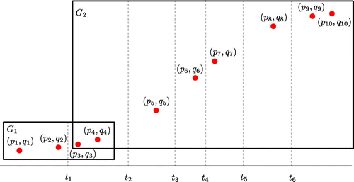
First, consider the subgroup G1. Note that this subgroup has two subintervals and is classified as T1. According to Algorithm 1, the modified $C$-test needs to be conducted for G1. From the simple calculation$$\begin{array}{c}\hfill C(p_1,q_1,p_2,q_2,p_3,q_3)\times C(p_2,q_2,p_3,q_3,p_4,q_4)=6.8894\times {10}^{-7}>0,\end{array}$$there exist $t_1,$${\mathit{\theta }}_1$ and ${\mathit{\theta }}_2$ for the solution $u(t)$ of Equation (2), as shown in Lemma 4.2.

Similarly, the second group G2 has six subintervals and is classified as T1. Here, of course, two data points $(p_3,q_3)$ and $(p_4,q_4)$ are common elements of G1 and G2. The subgroup G2 is also T1, and therefore the modified $C$-test is again needed. Since$$\begin{array}{c}\hfill C(p_4,q_4,p_5,q_5,p_6,q_6)\times C(p_5,q_5,p_6,q_6,p_7,q_7)=2.7138\times {10}^{-7}>0,\end{array}$$the existence of time nodes and parameters in G2 is guaranteed. Then the results shown in Table 2 can be obtained by applying a minimization scheme to minimize the functional (1818 $$\begin{array}{c}\hfill {\displaystyle f(t_1,\dots ,t_{n-1})=\sum _{i=1}^{n-1}{({\mathit{\theta }}_{i-1}-{\mathit{\theta }}_i)}^2,}\end{array}$$18 ).

Table 2. Minimization results for the functional (18) for data-set 1.

$j$	0	1	2	3	4	5	6	7
$t_j$	0.10000	0.22691	0.36204	0.46342	0.55737	0.60754	0.77273	0.90000
${\mathit{\theta }}_j$	9.31914	8.84667	7.15449	5.46094	3.76750	2.07546	0.38248

With estimated time nodes and parameters, the $L_2$ error between the derived and exact solutions of (2) is $1.7055\times {10}^{-2}$. Figure 5 shows the graph of the solutions.

Figure 5. The dashed line indicates the exact solution of (2020 $$\begin{array}{c}\hfill \frac{du}{dt}=ru(1-\frac{u}{K})\text{for}t\in (p_1,p_{10})\text{and}u(p_1)=u_0,\end{array}$$20 ), the solid line is the derived solution and dots represent data points.

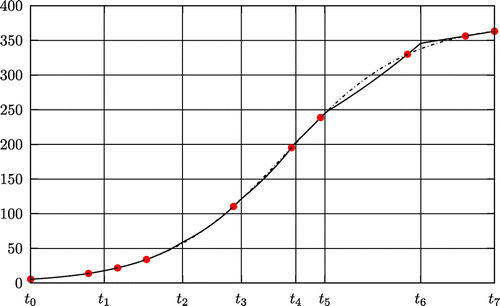
Table 3. Simulated data in data-set 2.

j	1	2	3	4	5	6	7	8	9	10
$p_j$	-0.90	-0.75	-0.55	-0.45	-0.20	0.00	0.25	0.30	0.60	0.85
$q_j$	0.7843	0.8688	0.9461	0.9701	0.9973	1.00	1.0052	1.0090	1.0747	1.2272

Figure 6. Given information in data-set 2 (dots represent data points).

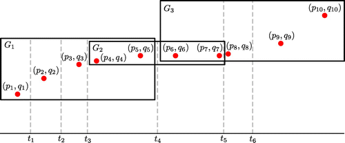
Table 4. Minimization results for the functional (18) for data set 2.

$j$	0	1	2	3	4	5	6	7
$t_j$	-0.90000	-0.75750	-0.59574	-0.34737	-0.00000	0.28494	0.59400	0.85000
${\mathit{\theta }}_j$	0.69334	0.47768	0.25085	0.013339	0.020822	0.20346	0.53083

Figure 7. The dashed line indicates the exact solution of (2121 $$\begin{array}{c}\hfill \frac{du}{dt}=t^{2}u\text{in}(p_1,p_{10})\text{and}u(p_1)=exp(p_1^3/3).\end{array}$$21 ), the solid line is the derived solution and dots represent data points.

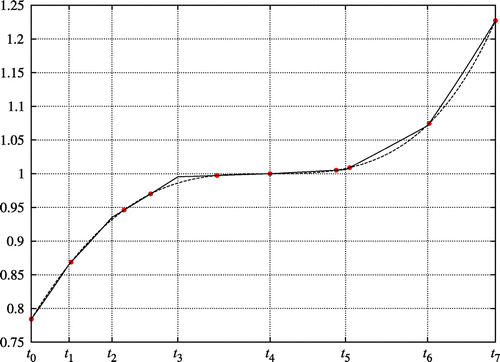
6.2 Data-set 2

Data-set 2 generates ${\{p_j\}}_{j=1}^{10}$ as random numbers in $[-1,1]$ and ${\{q_j\}}_{j=1}^{10}$ by solving the following differential equation at $p_j$:21 $$\begin{array}{c}\hfill \frac{du}{dt}=t^{2}u\text{in}(p_1,p_{10})\text{and}u(p_1)=exp(p_1^3/3).\end{array}$$21 The generated data-set ${\{(p_j,q_j)\}}_{j=1}^{10}$ is shown in Table 3. Data-set 2 considers seven subintervals ($I=7$), and the structure of subintervals is (1, 1, 1, 2, 2, 1, 2). In other words, the fourth, fifth and seventh subintervals have two data points, whereas the others, one data point. As depicted in Figure 6, the whole interval can be decomposed by three subgroups G1, G2 and G3. The first subgroup G1 has four subintervals and is classified as T2. In this case, there is no need to conduct the modified $C$-test because it is T2, and therefore the existence of time nodes and corresponding parameters are always guaranteed. On the other hand, G2 and G3 have two and three subintervals, respectively, and both are classified as T1. Therefore, the modified $C$-test needs to be conducted. In G2, however, the value of$$\begin{array}{c}\hfill C(p_4,q_4,p_5,q_5,p_6,q_6)\times C(p_5,q_5,p_6,q_6,p_7,q_7)=-1.8281\times {10}^{-6}\end{array}$$is negative, implying the nonexistence of $t_4$. Accordingly, it is not possible to determine a piecewise constant parameter function $\mathit{\theta }(t)$ satisfying (2) with this structure.

Consider another structure of subintervals. Suppose that seven subintervals ($I=7$) are given and the structure of subintervals is (1, 1, 2, 1, 2, 1, 2). In this case, the third, fifth and seventh subintervals have two data points, whereas the others, one data point. The whole interval can be decomposed into three subgroups G1, G2 and G3. As in the cases of the other data-sets, the modified $C$-test needs to be conducted for G2 and G3, which are of T1 type. Here simple calculations indicate that the modified $C$-test is successful, and therefore the optimal parameter function can be calculated. Table 4 shows the results. In addition, the $L_2$ error between the derived and exact solutions of (2121 $$\begin{array}{c}\hfill \frac{du}{dt}=t^{2}u\text{in}(p_1,p_{10})\text{and}u(p_1)=exp(p_1^3/3).\end{array}$$21 ) is $4.9836\times {10}^{-3}.$ Figure 7 shows the graph of the solutions with estimated time nodes and parameters.

7 Funding

This research was supported by NRF of Korea [grant number 2011-0000344], [grant number 2009-0065241], [grant number 2008-C00043].

Details of calculation in Lemma 4.3

 $$\begin{array}{cc}\hfill f(p_2,p_3)& {\displaystyle =[\frac{log{q}_1-log{q}_2}{p_1-p_2}-\frac{log{q}_4-log{q}_5}{p_4-p_5}]p_2{p}_3}\hfill \\ & {\displaystyle -[\frac{log{q}_1-log{q}_2}{p_1-p_2}{p}_3-log{q}_3+\frac{p_{4}log{q}_5-p_{5}log{q}_4}{p_4-p_5}]p_2}\hfill \\ & {\displaystyle +[\frac{p_{1}log{q}_2-p_{2}log{q}_1}{p_1-p_2}-log{q}_3+\frac{log{q}_4-log{q}_5}{p_4-p_5}{p}_3]p_3}\hfill \\ & {\displaystyle -[\frac{p_{1}log{q}_2-p_{2}log{q}_1}{p_1-p_2}-\frac{p_{4}log{q}_5-p_{5}log{q}_4}{p_4-p_5}]p_3}\hfill \\ & =\frac{p_2{p}_3-p_2{p}_3-p_2{p}_3+p_2{p}_3}{p_1-p_2}log{q}_1-\frac{p_2{p}_3-p_2{p}_3-p_1{p}_3-p_1{p}_3}{p_1-p_2}log{q}_2\hfill \\ & -(p_3-p_2)log{q}_3-\frac{p_2{p}_3-p_2{p}_5-p_3^2+p_3{p}_5}{p_4-p_5}log{q}_4\hfill \\ & +\frac{p_2{p}_3-p_2{p}_4-p_3^2+p_3{p}_4}{p_4-p_5}log{q}_5\hfill \\ & =(p_2-p_3)log{q}_3-\frac{(p_2-p_3)(p_3-p_5)}{p_4-p_5}log{q}_4+\frac{(p_2-p_3)(p_3-p_4)}{p_4-p_5}log{q}_5\hfill \\ & =\frac{p_2-p_3}{p_4-p_5}\times C(p_3,q_3,p_4,q_4,p_5,q_5),\hfill \end{array}$$$$\begin{array}{cc}\hfill f(p_2,p_4)& {\displaystyle =[\frac{log{q}_1-log{q}_2}{p_1-p_2}-\frac{log{q}_4-log{q}_5}{p_4-p_5}]p_2{p}_4}\hfill \\ & {\displaystyle -[\frac{log{q}_1-log{q}_2}{p_1-p_2}{p}_3-log{q}_3+\frac{p_{4}log{q}_5-p_{5}log{q}_4}{p_4-p_5}]p_2}\hfill \\ & {\displaystyle +[\frac{p_{1}log{q}_2-p_{2}log{q}_1}{p_1-p_2}-log{q}_3+\frac{log{q}_4-log{q}_5}{p_4-p_5}{p}_3]p_4}\hfill \\ & {\displaystyle -[\frac{p_{1}log{q}_2-p_{2}log{q}_1}{p_1-p_2}-\frac{p_{4}log{q}_5-p_{5}log{q}_4}{p_4-p_5}]p_3}\hfill \\ & =\frac{p_2{p}_4-p_2{p}_3-p_2{p}_4+p_2{p}_3}{p_1-p_2}log{q}_1-\frac{p_2{p}_4-p_2{p}_3-p_1{p}_4+p_1{p}_3}{p_1-p_2}log{q}_2\hfill \\ & -(p_4-p_2)log{q}_3-\frac{p_2{p}_4-p_2{p}_5-p_3{p}_4+p_3{p}_5}{p_4-p_5}log{q}_4\hfill \\ & +\frac{p_2{p}_4-p_2{p}_4-p_3{p}_4+p_3{p}_4}{p_4-p_5}log{q}_5\hfill \\ & =-(p_3-p_4)log{q}_2-(p_4-p_2)log{q}_3-(p_2-p_3)log{q}_4\hfill \\ & =-C(p_2,q_2,p_3,q_3,p_4,q_4),\hfill \end{array}$$

References

- Beck JV, Arnold KJ. Parameter estimation in engineering and science. New York (NY): John Wiley & Sons; 1977.
- Tarantola A. Inverse problem theory. Methods for data fitting and model parameter estimation. Amsterdam: Elsevier; 1987.
- Banks HT, Bihari KL. Modelling and estimating uncertainty in parameter estimation. Inverse Probl. 2001;17:95–111.
- Banks HT, Fitzpatrick BG. Statistical methods for model comparison in parameter estimation problems for distributed systems. J. Math. Biol. 1990;28:501–527.
- Hvala N, Zec M, Strmc̆nik S. Non-linear model parameter estimation-estimating a feasible parameter set with respect to model use. Math. Comput. Modell. Dyn. Syst. Meth. Tools Appl. Eng. Related Sci. 2008;14:587–605.
- Martinsons CD. Optimal parameterization of a mathematical model for solving parameter estimation problems. Inverse Probl. Sci. Eng. 2005;13:109–131.
- Seber GAF, Wild CJ. Nonlinear regression. Hoboken (NJ): Wiley-Interscience; 2003.
- Beverton RJH, Holt SJ. A review of the lifespans and mortality rates of fish in nature, and their relation to growth and other physiological characteristics. Chichester: John Wiley & Sons Ltd; 2008. p. 142–180.
- Cren EDL. The length-weight relationship and seasonal cycle in gonad weight and condition in the perch (perca fluviatilis). J. Animal Ecol. 1951;20:201–219.
- White P, Kalff J, Rasmussen J, Gasol J. The effect of temperature and algal biomass on bacterial production and specific growth rate in freshwater and marine habitats. Microb. Ecol. 1991;21:99–118.
- Aiello WG, Freedman H. A time-delay model of single-species growth with stage structure. Math. Biosci. 1990;101:139–153.
- Aiello WG, Freedman HI, Wu J. Analysis of a model representing stage-structured population growth with state-dependent time delay. SIAM J. Appl. Math. 1992;52:855–869.
- Gourley SA, Kuang. Y. A stage structured predator-prey model and its dependence on maturation delay and death rate. J. Math. Biol. 2004;49:188–200.
- Gurney WSC, Nisbet RM. Fluctuation periodicity, generation separation, and the expression of larval competition. Theoret. Population Biol. 1985;28:150–180.
- Nisbet RM, Blythe SP, Gurney WSC, Metz JAJ. Stage-structure models of populations with distinct growth and development processes. IMA J. Math. Appl. Med. Biol. 1985;2:57–68.
- Rockafellar RT. The multiplier method of Hestenes and Powell applied to convex programming. J. Optim. Theory Appl. 1973;12:555–562.
- Gauze GF. The struggle for existence. Baltimore (MD): The Williams & Wilkins company; 1934.