Identification of linear and non-linear physical parameters of multistory shear buildings using artificial neural network

Abstract

In this research, a novel method has been proposed for simultaneous identification of physical parameters (i.e. mass, stiffness and damping matrices) as well as for separation of linear physical parameters from non-linear ones by use of artificial neural networks (ANNs) in non-linear multi-degree-of-freedom (DOF) systems. To design an appropriate ANN in this method, the vibration equation of the lumped mass system is re-arranged into a new form. The proposed ANN has two parts; namely linear and non-linear. The outputs of the non-linear part of the proposed ANN identify the non-linear properties of the system. Moreover, the number of the employed ANNs is equal to the number of DOFs considered for the non-linear system. Initially, the first ANN is trained and the corresponding parameters of the linear part are then identified. Afterwards, the second ANN is trained using the identified mass of the first DOF. This procedure of training and identifying the parameters of each DOF is repeated in this manner until all DOF parameters are identified; then the identification of the non-linear part begins by exciting the non-linear part of ANN. Finally, the linear stiffness values and non-linear patterns are obtained from the output results of the excitations. The proposed algorithm has been verified through some examples.

Keywords:

• Mass–damping–stiffness identification
• linear and non-linear identification
• inverse problems
• shear building model
• forced vibration
• artificial neural networks

1. Introduction

To record non-linear hysteresis cycles of structures, one has to wait for earthquakes to occur. On the other hand, to identify structures by forced vibration methods,[1] an actual structure cannot be excited so that the non-linear cycles may be recorded, as strong excitations may lead to structural damage. The non-linear behaviour may be observed in structures due to factors such as infill non-structural elements, structural damages and various elements with non-linear behaviour.[2] In the linear parameters’ identification with the presence of non-linearity, non-linear factors may be considered and recognized with an appropriate non-linear pattern. In this approach, non-linear factors are considered as a non-Gaussian noise in the system. The history of non-linear identification roots back to 1970s and to the principal works of Ibáñez.[3] Since then, the development of the non-linear identification methods has led to the publication of several text books. One of the first books published in this field was authored by Worden and Tomlinson.[4] Moreover, there are some other books based on the Bouc–Wen model written in recent years.(see e.g. Ref. [5]) There are various approaches in the field of identification of non-linear multi-degree-of-freedom (MDOF) systems. One of these approaches is identified with reduction of the number of DOFs used in data acquisition. Platten et al. [6] applied the extended modal space model to the identification of non-linear MDOFs systems with excitation of some specific DOFs. In non-linear identification, one may use a predefined pattern to decrease the indeterminacy in non-linear systems. Xueqi et al. [7] proposed a method to identify non-linear systems by a piecewise linear pattern. Zhang et al. [8] employed three methods to identify non-linear systems assuming that the non-linear behaviour of the model follows that of the Bouc-Wen’s.

The identification of systems may be performed in the frequency or the time domain. Due to the course of development in the control science, the time domain methods have been more variable and prevalent than the frequency domain ones. A group of common methods called as non-linear autoregressive moving average model with exogenous inputs family can be used for solving a wide range of time domain problems, owing to their nature being based on time history windows.[9] Another common time domain method is Kalman Filtering. Ghanem and Ferro [10] utilized this tool to identify non-linear systems in the field of health monitoring. Their proposed non-linear model is similar to Bouc-Wen model. The Kalman Filter method has been introduced in a branch of the modern control science; therefore, health monitoring and damage detection have brought it more into play in sub-branches of system identification.[11] In recent years, some non-linear identification based on least square (LS) methods has been carried out by Yang and his co-workers.[12,13] In addition, some methods have been created by the combination of time-domain and frequency domain-methods.[14]

In addition to numerous approaches in the field of non-linear system identification which are based on hard computing methods, there are other approaches which are in accordance with soft computing methods; particularly those based on artificial intelligence.[15,16] The advantage of intelligence-based methods, such as those based on artificial neural network (ANN), is that the solution procedure is independent from complex mathematical equations or even from recursive trends. The purpose of the present study is to obtain the linear parameters as well as to estimate the non-linear patterns of structures. In this method, the required vibrations are not so strong. In this regard, some parts of the equation solving procedure are achieved using ANN. The proposed method of this research does not require any predefined patterns beyond the common methods. Besides, this method can be used in the fields of damage detection and system identification, owing to its potential to recognize non-linear patterns.

2. Linear and non-linear single DOF system identification

In this section, a system identification method based on ANN, which is able to separate linear terms from non-linear ones, is proposed. At first a single DOF system is identified and then the proposed method will be generalized to multi DOF systems. The behaviour of a single DOF system may be given by(1) $$m\ddot{x}(t)+c\dot{x}(t)+kx(t)+h\left(x(t),\dot{x}(t)\right)=f(t)$$(1)

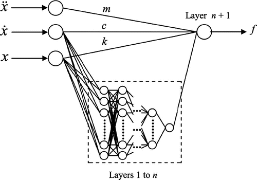
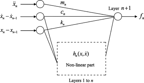
in which m, c and k represent unknown structural parameters of mass, damping and stiffness, respectively, that should be identified uniquely. Furthermore, $x(t)$, $\dot{x}(t)$ and $\ddot{x}(t)$ indicate known displacement, velocity and acceleration values, respectively. In addition, $h\left(x(t),\dot{x}(t)\right)$ denotes the non-linear part of the system. Figure 1 illustrates the proposed ANN identification scheme to find the linear part of Equation (1).

Figure 1. The proposed ANN architecture for the identification of linear and non-linear terms.

The most popular method for learning in multi-layer neural networks is called back-propagation (BP). It was first invented in 1969 by Bryson and Ho [17], but was largely ignored until the mid-1980s.[18–20] The name of BP was firstly coined by Rumelhart et al. [21]. The proposed ANN of Figure 1 employs a non-linear BP multi-layer neural network which is supposed to identify the non-linear term $h\left(x(t),\dot{x}(t)\right)$. The layer $n+1$ is a neuron with a linear threshold function which is only used for weighted sum of the input signals feeding input to this neuron, while the other neurons have the sigmoid threshold function. It should be noted that the sigmoid functions are very similar to the input–output relationships of typical biological neurons.[15] Furthermore, the derivatives of sigmoid functions may be easily calculated, which is helpful for function approximation. The number of layers and neurons in each layer as well as the training ratio depend upon the primary assumption and are improved at the next recursion of the training phase. In this research, the application of the proposed method is limited to dynamical systems that have only a non-linear term in x. In other words, the simultaneous identification of non-linear x and non-linear $\dot{x}$ turns out to undesirable identified patterns. In fact, the ANN will get trapped in a local optimum. If we know which of these two parameters (x or $\dot{x}$) have more influence on the behaviour of the structure, it will help us to perform a more suitable identification. In addition, supervised learning is selected as the ANN’s learning rule for all examples of the present research.[19]

2.1. Example 1

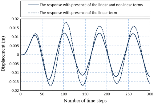
As the first example, a one-story shear building is considered. Mass, stiffness and damping of the building are equal to 1000 Ns² m⁻¹, 120,000 N m⁻¹ and 3300 N m⁻¹ s, respectively. Moreover, the non-linear term is assumed to be 250,000,000$x^3$. This structure has been excited by a harmonic vibration with a frequency of 1.27 Hz and sampling rate of 100 Hz. Figure 2 shows both linear and non-linear responses. In this figure, linear response is obtained by elimination of the non-linear term of the model. Obviously, in this case study the non-linear term makes the system stiffer almost in all time steps. Hence, existence of the non-linear term has affected the structural responses. This effect on the structural response cannot be neglected.

Figure 2. The response of the first example with or without presence of the non-linear term.

Solving this problem via the classical LS method will lead to the answers demonstrated in Table 1. The well-known LS method is a linear identification method that provides a rough estimation of the accurate solution. For this example, a cubic polynomial is used to estimate the accurate solution of the problem. As shown in Table 1, the mass of the structure has been estimated with about 25% error compared to its accurate value, which is not acceptable for this single DOF system. In other words, small inaccuracy at this single DOF will propagate as the proposed method is generalized to multi-DOFs, which may lead to substantially large errors in identification of physical parameters therein.

Table 1. The first example: estimation of the corresponding physical parameters by the LS method. For this table, equation $[[M]⋮[C]⋮[K]][Y]={[F]}_{}$ is used to identify the physical parameters.

	Accurate	Estimated
Mass (Ns^2 m^−1)	1000	746
Stiffness (N m^−1)	120,000	128,300
Damping (N m^−1 s)	3300	3423

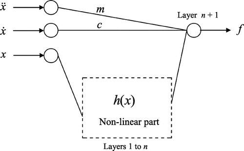
Now let us suppose that the displacement has a non-linear behaviour, while the velocity remains linear. Note that the supposition of non-linear stiffness and linear damping is a logical assumption in the buildings. By using ANN for identification, the mass and damping identifications have been assigned to the linear part of the proposed ANN, while both linear and non-linear stiffness identifications will be performed by the non-linear part of the proposed ANN (see Figure 3).

Figure 3. Proposed ANN for the identification of non-linear systems.

The non-linear part of the ANN consists of five layers. The number of the neurons in the layers is 8, 4, 3, 2 and 2, respectively. The important point in training this specific ANN is that the common normalizations, in popular practice of ANN training, must be avoided in the training data. Due to the existence of a linear part in the ANN, normalisation may lead to undesirable weight training. Instead of data normalisation, one is supposed to define lower and upper limits for the input data. In this case study, supposing the ANN gets trained correctly, one may expect that the weights of the non-linear neural network identify a polynomial of third order. In Table 2, the mass and damping values have been directly obtained from the weights of the linear part in the trained ANN of Figure 3.

Table 2. The first example: estimation of corresponding physical parameters by the ANN method shown in Figure 1.

	Accurate	Estimated
Mass (Ns^2 m^−1)	1000	1014
Stiffness (N m^−1)	120,000	123,000
Damping (N m^−1 s)	3300	3366

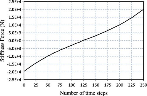
As previously mentioned, the identification of linear and non-linear stiffness values has been assigned to the non-linear part of the ANN. Therefore, the stiffness value cannot be directly presented in the form of identified model of the system shown in Figure 3. In order to extract the linear stiffness, one has to first apply the appropriate input data to the ANN of Figure 3. For this purpose, the subsequent identification steps are as follows: (a) separating the non-linear part of the trained ANN from its linear part; (b) identification of the separated non-linear part by applying an input vector starting from a lower limit and ending with an upper one. In this example, the lower and upper limits are selected as −0.0125 and +0.0125, respectively. As already discussed, the input of the network is displacement, and hence the mentioned limits have been obtained by considering the average maximum displacement with the presence of the linear and non-linear terms (see Figure 2). The chosen values are the minimum and maximum response values of the system, which has been linearly divided into 250 time steps of identical increasing rate. Output values of the ANN are corresponding to the stiffness force of the problem as illustrated in Figure 4. This figure depicts a third-order polynomial as predicted from $kx(t)+h\left(x(t),\dot{x}(t)\right)$ terms of Equation (1).

Figure 4. Non-linear pattern investigation by the proposed ANN.

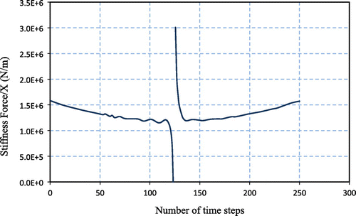
Both linear and non-linear stiffness patterns may be identified using the non-linear part of the ANN through dividing the output values by the input values (see Figure 5). The linear stiffness should be obtained by taking the average values adjacent to the 125th time step, after eliminating the large values which are resulted from dividing by an infinitesimal value. In fact, the linear stiffness is equal to the limit of the function shown in Figure 5, as the time step approaches to the 125th one. The estimated linear stiffness is 123,000 N m⁻¹ which involves only 2.4% errors. In the next section, the idea of applying ANN is generalised to the identification of physical parameters for multistory shear buildings.

Figure 5. Estimation of the linear stiffness.

3. Algorithm of the proposed identification method

In this section, the proposed identification algorithm which involves the following principal steps is introduced^{Figure 3}:^{Figure 6}

• Step 1: Model selection: The model should include two major linear and non-linear parts. For this purpose, we select the connection between the two major parts and neurons based on the vibration equation. We then select the number of ANN’s layers as well as neurons of each layer. As may be shown later, in this step, two different ANN’s architectures could be selected (see Figures 3 and 6).

• Step 2: Data selection: The identification needs a database including forced vibration, displacement, and its first and second derivatives at the same time step.

• Step 3: Training the proposed ANN model: In the present algorithm, the back-propagation training method is adopted. It should be noted that the noise of experimental data is removed before training. To this end, by using high-order finite impulse response filters, undesirable effects of noises may partially be eliminated from training data.[22,23]

• Step 4: Separation: The non-linear part is separated from the general model of the trained ANN model. In fact, the mass is directly identified in this step. Assuming that the structural damping is linear, it is directly identified in this step. At the end of this step, two various cases may occur:

  • (4a) if the selected architecture of step 1 is similar to Figure 3, the linear stiffness is identified;

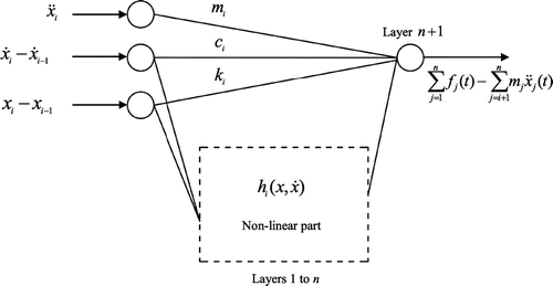
  • (4b) if the selected architecture of step 1 is the same as Figure 6, both linear and non-linear parameters may be identified in step 5.

• Step 5: Non-linear identification: Identification of the separated non-linear part of the model by using applied appropriate input vectors and interpretation of output diagrams.

Figure 6. The proposed ANN for the identification of the nth DOF.

These steps will be described in more details in the examples of following section.

4. Linear and non-linear multi DOF system identification

Let us consider a shear building structural system with n story, governed by the following equation:(2) $$[M]{\{\ddot{X}\}}_t+[C]{\{\dot{X}\}}_t+[K]{\{X\}}_t+\{H({\{X\}}_t,{\{\dot{X}\}}_t)\}={\{F\}}_t$$(2)

where ${\{\ddot{X}\}}_t$, ${\{\dot{X}\}}_t$ and ${\{X\}}_t$ indicate known acceleration, velocity and displacement vectors, respectively. Moreover,(3) $$[M]=\text{diag}[\begin{array}{ccccc}{m}_1& m_2& \cdots & m_{n-1}& m_n\end{array}],$$(3) (4) $$[C]=\left[\begin{array}{ccccc}{c}_1+c_2& -c_2& \cdots & 0& 0\\ -c_2& c_2+c_3& \cdots & 0& 0\\ ⋮& ⋮& \ddots & ⋮& ⋮\\ 0& 0& \cdots & c_{n-1}+c_n& -c_n\\ 0& 0& \cdots & -c_n& c_n\end{array}\right],$$(4) (5) $$[K]=\left[\begin{array}{ccccc}{k}_1+k_2& -k_2& \cdots & 0& 0\\ -k_2& k_2+k_3& \cdots & 0& 0\\ ⋮& ⋮& \ddots & ⋮& ⋮\\ 0& 0& \cdots & k_{n-1}+k_n& -k_n\\ 0& 0& \cdots & -k_n& k_n\end{array}\right].$$(5)

Furthermore, ${\{F\}}_t$ and $\{H({\{X\}}_t,{\{\dot{X}\}}_t)\}$ are recorded excitations and unknown non-linear parameter vectors, respectively.

In order to employ Equation (2) for system identification purpose using the proposed ANN model, the equation can be written as:(6) $${[M]}_{n\times n}{[\ddot{X}]}_{n\times np}+{[C]}_{n\times n}{[\dot{X}]}_{n\times np}+{[K]}_{n\times n}{[X]}_{n\times np}+{[H]}_{n\times np}={[F]}_{n\times np}$$(6)

in which $np$ denotes the number of time windows on the displacement, velocity and acceleration matrices, which in turn show the state of the dynamic system. The linear and non-linear parameters of Equation (6) can be separated using the following compact form:(7) $${[[M]⋮[C]⋮[K]]}_{n\times 3n}{\left[\begin{array}{c}[\ddot{X}]\\ [\dot{X}]\\ [X]\end{array}\right]}_{3n\times np}+{[H]}_{n\times np}={[F]}_{n\times np}$$(7)

or(8) $${[A]}_{n\times 3n}{[Y]}_{3n\times np}+{[H]}_{n\times np}={[F]}_{n\times np}$$(8)

where(9) $$[A]=[[M]⋮[C]⋮[K]],[Y]=\left[\begin{array}{c}[\ddot{X}]\\ [\dot{X}]\\ [X]\end{array}\right].$$(9)

In order to solve Equation (8) to estimate the unknown matrix $[A]$, different hard-computing (e.g. singular value decomposition) and/or soft-computing (e.g. ANNs and Genetic Algorithms) methods may appear to be efficient.[22,23] As it is obvious from Equation (9), the dimensions of known $[Y]$ matrix are very large. As a result, direct application of hard- and/or soft-computing methods may provide meaningless results for unknown parameters.[24,25] To resolve this problem, a new method is presented in this research. To illustrate the details of proposed formulation, a shear building of n DOF is considered. For this case, the following set of equations may be rewritten from Equations (2)–(5):(10) $$m_1{\ddot{x}}_1(t)+(c_1+c_2){\dot{x}}_1(t)-c_2{\dot{x}}_2(t)+(k_1+k_2)x_1(t)-k_2{x}_2(t)+h_1(x_1(t),{\dot{x}}_1(t))-h_2(x_2(t)-x_1(t),{\dot{x}}_2(t)-{\dot{x}}_1(t))=f_1(t)$$(10)

and(11) $$m_i{\ddot{x}}_i(t)-c_i{\dot{x}}_{i-1}(t)+(c_i+c_{i+1}){\dot{x}}_i(t)-c_{i+1}{\dot{x}}_{i+1}(t)-k_i{x}_{i-1}(t)+(k_i+k_{i+1})x_i(t)-k_{i+1}{x}_{i+1}(t)+h_i\left(x_i(t)-x_{i-1}(t),{\dot{x}}_i(t)-{\dot{x}}_{i-1}(t)\right)-h_{i+1}\left(x_{i+1}(t)-x_i(t),{\dot{x}}_{i+1}(t)-{\dot{x}}_i(t)\right)=f_i(t)$$(11)

for $i=2,3,\dots ,n-1$.

Finally, for the nth DOF, one may write(12) $$m_n{\ddot{x}}_n(t)-c_n{\dot{x}}_{n-1}(t)+c_n{\dot{x}}_n(t)-k_n{x}_{n-1}(t)+k_n{x}_n(t)+h_n(x_n(t)-x_{n-1}(t),{\dot{x}}_n(t)-{\dot{x}}_{n-1}(t))=f_n(t)$$(12)

As the main purpose of the present method is direct estimation of structural parameters, Equation (12) may be given by(13) $$m_n{\ddot{x}}_n(t)+c_n[{\dot{x}}_n(t)-{\dot{x}}_{n-1}(t)]+k_n[x_n(t)-x_{n-1}(t)]+h_n(x_n(t)-x_{n-1}(t),{\dot{x}}_n(t)-{\dot{x}}_{n-1}(t))=f_n(t)$$(13)

Employing the information of previous $np$ time steps, Equation (13) can be solved using the proposed ANN of Figure 1. The inputs of this network are structural acceleration, relative velocity and relative displacement of the nth story, respectively. The output of the network is the applied force at time t. While solving Equation (13) using this network, the training process is achieved using $np$ training patterns. Afterwards, by setting the weighting matrix of the ANN, the corresponding components of this matrix indicate the unknown $m_n$, $c_n$ and $k_n$ parameters, respectively. At the next step, the mass of the nth story is used in the identification of the ($n-1$)th story. Assuming that the parameters of the nth story are identified values, Equation (11) is written as:(14) $$m_i{\ddot{x}}_i(t)+c_i\left({\dot{x}}_i(t)-{\dot{x}}_{i-1}(t)\right)+k_i\left(x_i(t)-x_{i-1}(t)\right)+h_i\left(x_i(t)-x_{i-1}(t),{\dot{x}}_i(t)-{\dot{x}}_{i-1}(t)\right)=f_i(t)+c_{i+1}\left({\dot{x}}_{i+1}(t)-{\dot{x}}_i(t)\right)+k_{i+1}\left(x_{i+1}(t)-x_i(t)\right)+h_{i+1}\left(x_{i+1}(t)-x_i(t),{\dot{x}}_{i+1}(t)-{\dot{x}}_i(t)\right)$$(14)

or(15) $$m_i{\ddot{x}}_i(t)+c_i\left({\dot{x}}_i(t)-{\dot{x}}_{i-1}(t)\right)+k_i\left(x_i(t)-x_{i-1}(t)\right)+h_i\left(x_i(t)-x_{i-1}(t),{\dot{x}}_i(t)-{\dot{x}}_{i-1}(t)\right)=f_i(t)+f_{i+1}(t)-m_{i+1}{\ddot{x}}_{i+1}(t)$$(15)

in which, $i=n-1$, and all parameters of right-hand side of Equation (15) are identified. Equation (15) is solved by using an ANN with similar topology as the former one used for the nth story. The corresponding components of weighting matrix of linear part of this network present the unknown $m_i$, $c_i$ and $k_i$ parameters. At the final step, the unknown parameters of the first story are determined using the same procedure as the second story. Therefore, in general form (for $i=2,3,\dots ,n-1$), Equation (15) may be written as(16) $$m_i{\ddot{x}}_i(t)+c_i\left({\dot{x}}_i(t)-{\dot{x}}_{i-1}(t)\right)+k_i\left(x_i(t)-x_{i-1}(t)\right)+h_i\left(x_i(t)-x_{i-1}(t),{\dot{x}}_i(t)-{\dot{x}}_{i-1}(t)\right)=\sum _{j=i}^n{f}_j(t)-\sum _{j=i+1}^n{m}_j{\ddot{x}}_j(t)$$(16)

Moreover, Equation (16) may be used for the first story (for $i=1$), if we assume that $x_0={\dot{x}}_0={\ddot{x}}_0=0$. All equations used in the present identification method can be summarised in the following matrix form(17) $$\begin{array}{c}\left[\begin{array}{cccccccccccccc}{m}_1& 0& \cdots & 0& |& c_1& 0& \cdots & 0& |& k_1& 0& \cdots & 0\\ 0& m_2& \cdots & 0& |& 0& c_2& \cdots & 0& |& 0& k_2& \cdots & 0\\ ⋮& ⋮& \ddots & ⋮& |& ⋮& ⋮& \ddots & ⋮& |& ⋮& ⋮& \ddots & ⋮\\ 0& 0& \cdots & m_n& |& 0& 0& \cdots & c_n& |& 0& 0& \cdots & k_n\end{array}\right]\hfill \\ \times {\left\{\begin{array}{c}{\ddot{x}}_1\hfill \\ {\ddot{x}}_2\hfill \\ ⋮\hfill \\ {\ddot{x}}_n\hfill \\ {\dot{x}}_1\hfill \\ {\dot{x}}_2-{\dot{x}}_1\hfill \\ ⋮\hfill \\ {\dot{x}}_n-{\dot{x}}_{n-1}\hfill \\ x_1\hfill \\ x_2\hfill \\ ⋮\hfill \\ x_n-x_{n-1}\hfill \end{array}\right\}}_{(t)}+{\left[\begin{array}{c}{h}_1(x_1,{\dot{x}}_1)\\ h_2(x_2-x_1,{\dot{x}}_2-{\dot{x}}_1)\\ ⋮\\ h_n(x_n-x_{n-1},{\dot{x}}_n-{\dot{x}}_{n-1})\end{array}\right]}_{(t)}\hfill \\ ={\left\{\begin{array}{c}{f}_1+f_2+\cdots +f_n-m_2{\ddot{x}}_2-\cdots -m_n{\ddot{x}}_n\\ f_2+f_3+\cdots +f_n-m_3{\ddot{x}}_3-\cdots -m_n{\ddot{x}}_n\\ ⋮\\ f_n\end{array}\right\}}_{(t)}\hfill \end{array}$$(17)

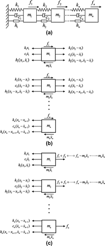
The above set of equations is schematically illustrated in Figure 7. Now, the former mathematical form of Equation (17) may be easily examined using an ANN representation as shown in Figure 6, in which a general ANN identification form is depicted.

Figure 7. The schematic illustration of Equation (17): (a) the equivalent mass–stiffness–damper system, (b) the common form of vibration equations and (c) re-arrangement form of vibration equations.

The identification of the ANN shown in Figure 6 may result in the physical parameters of the nth DOF (or story). Now, using the subsequent $m_n$, a new ANN is used for identification of the ($n-1$)th story. Figure 8 illustrates the inputs and outputs of the ANN designed to identify the physical parameters of the ith story. The physical parameters of the first story can be calculated by changing the inputs and outputs of the same network based on Figure 6 as shown in Figure 8.

Figure 8. The proposed ANN for the identification of the ith DOF.

It should be noted that all neurons of input layer are connected to the next layer. Actually, this configuration (i.e. the relation between mass, spring, damper and the non-linear part of the model) is selected based on the mathematics of the problem, which is shown in Equation (17). In other words, neurons’ connections are deleted wherever the components of the right matrix of Equation (17) are zero. The main concern now would be to choose the optimum number of layers and neurons for the non-linear part of the model. It is important to note that we are actually able to estimate the total mass of each story in the building. In any building, the material used for construction is known, so we can directly calculate the mass of each story by implementation of known material’s volumes and densities. In the present approach, the mass of building has been assumed to be unknown. Therefore, the difference between the identified mass and the accurate mass as given by

(18) $$\text{Performance}\text{criterion}=\frac{M_{\text{Estimated}}-M_{\text{Accurate}}}{M_{\text{Accurate}}}\times 100$$(18)

is a good criterion to evaluate the precision of the neural network’s performance as well as to choose the number of layers and neurons. The present method is evaluated through some examples.

4.1. Example 2

As the second example, let us consider a three-story shear building whose linear characteristics are given in Table 3. The structure is excited by a harmonic loading of 1.27 Hz, and the associated structure responses are sampled by a frequency of 100 Hz. As already discussed, the identification of the ANN shown in Figure 6 results in the physical parameters of the nth DOF. The results of estimation using the proposed method are presented in Table 4. As may be observed from Table 4, the estimation results show very good agreement with the actual characteristics, especially for the mass and damping parameters.

Table 3. The second example: physical parameters of the three-story building.

	1st story	2nd story	3rd story
Mass (Ns^2 m^−1)	3000	3000	2000
Stiffness (N m^−1)	1.2E6	$0.8\text{E}6+1.3\text{E}11\times {(x_2-x_1)}^3$	$0.6\text{E}6+2.5\text{E}12\times {(x_3-x_2)}^3$
Damping (N m^−1 s)	8000	5000	4000

Table 4. The second example: estimation of physical parameters by the proposed method.

	1st story	2nd story	3rd story
Mass (Ns^2 m^−1)	3000.2	3000.2	2000.1
Stiffness (N m^−1)	1,200,000	800,100	618,380
Damping (N m^−1 s)	7998.6	4992.5	3998.9
Performance criteria	0.006	0.006	0.005

4.2. Example 3

Consider another three-story shear building with linear characteristics of Table 5. This structure is excited by a 7.96 Hz harmonic vibration and the structural response is sampled by a frequency of 100 Hz. The results of estimation by the proposed method are summarised in Table 6. As may be observed, the proposed method is capable of recognising the linear part and separating it from the non-linear one. The ANN presented in Figure 3 is employed for identification of the structure.

Table 5. The third example: physical parameters of the three-story building.

	1st story	2nd story	3rd story
Mass (Ns^2 m^−1)	3000	3000	2000
Stiffness (N m^−1)	1.2E6	$0.8\text{E}6+6.5\text{E}12\times {(x_2-x_1)}^3$	$0.6\text{E}6+1.25\text{E}14\times {(x_3-x_2)}^3$
Damping (N m^−1 s)	8000	5000	4000

Table 6. The third example: estimation of physical parameters by the proposed method.

	1st story	2nd story	3rd story
Mass (Ns^2 m^−1)	3000.9	2998.8	2000.5
Stiffness (N m^−1)	1,200,000	799,799	600,100
Damping (N m^−1 s)	7988.1	4998.8	4001.3
Performance criteria	0.03	−0.04	0.025

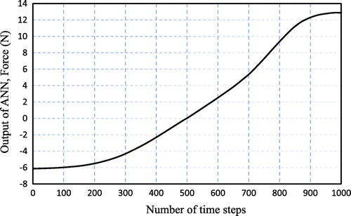
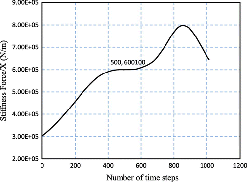
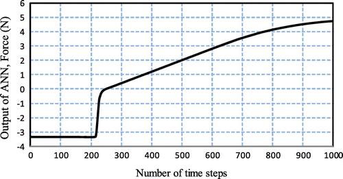
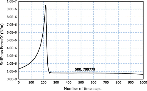
The method described in Section 3 is used to identify the structure. Furthermore, the architecture of ANN presented in Figure 3 is employed instead of the ANN shown in Figures 6 and 8. It should be noted that the topology illustrated in Figures 6 or 8 is not generally suitable for all examples. In fact, in this topology the linear and non-linear parts of the ANN compete against each other to minimise the error. Therefore, the linear coefficient is shared between linear and non-linear parts. The ANN architecture shown in Figure 3 is more general, and there is no competition between two parts. Consequently, the ANN architecture of Figure 3 employed to identify the non-linear part, in this example. When the training process is accomplished and the linear part of the ANN is separated from the primary neural network, an appropriate vector, within the training range, is assigned to the non-linear part. The third DOF output results corresponding to the non-linear part are illustrated in Figure 9. In this figure, the horizontal axis shows the time steps of the input data, while the vertical axis represents the output of the non-linear part of the proposed neural network. The result of division of the vertical values by the horizontal ones has been illustrated in Figure 10, which represents the stiffness values of the 3rd DOF. The value of the vertical axis at the vicinity of the 500th time step yields the linear stiffness of the third DOF (see Figure 10). For the second and first DOFs, the approach is identical to that of the third one. Figures 11 and 12 correspond to the second DOF, while its identification results are given in Table 6.

Figure 9. The output of non-linear part of the third DOF for the corresponding input vector.

Figure 10. The stiffness of the third DOF.

Figure 11. The output of non-linear part of the second DOF for the corresponding input vector.

Figure 12. The stiffness of the second DOF.

The 300 patterns of the training data including input and output vectors have been directly obtained by simulating the non-linear dynamic of structural model, and have been applied in the present work. Moreover, the parameters implemented in the simulation are mentioned in examples 1–3. The presented examples are simulated using a MATLAB programme provided by the authors. In this programme, the CPU time of examples 1, 2 and 3 are 32, 41 and 47 min, respectively. In this work, the training algorithm has been set to stop when the number of epochs exceeds 5000.

5. Conclusions

In this paper, a novel method based on ANN has been proposed for simultaneous identification of physical parameters as well as separation of linear physical parameters from the non-linear ones, for non-linear multi-DOF systems. This study has started with proposing a general method to identify a single-DOF system, and thereafter extended by developing the model for the multi-DOF system. At first, a single DOF with a non-linear term in its stiffness has been investigated and the obtained results of identification have shown the robustness of the proposed method. It should be noted that training data should not be normalised in order to achieve true identification.

Instead, three terminating criteria have been considered as follows to terminate the training procedure: (a) when the number of epochs exceeds predefined number, or; (b) when the neural network weights change less than a certain value or; (c) when changes in the weights gradient are small. Finally, to generalise the identification to multi DOF systems, the present study has stepped further to re-arrange the common vibration equation, and to be able to employ an upgraded version of the equation for the preceding method. Two more examples have been investigated to illustrate the method in more detail. As expected, the examples show that the estimated values of physical parameters are in very good agreement with the actual values and separate the linear stiffness of the system from its non-linear counterpart with adequate accuracy.

Acknowledgements

The authors would like to acknowledge and express their special gratitude to anonymous reviewers, for their constructive advice that improved the manuscript.

References

- Karimi I, Khaji N, Ahmadi MT, Mirzayee M. System identification of concrete gravity dams using artificial neural networks based on a hybrid FE–BE approach. Eng. Struct. 2011;32:3583–3591.
- Khaji N, Shafiei M, Jalalpour M. Closed-form solutions for crack detection problem of Timoshenko beams with various boundary conditions. Int. J. Mech. Sci. 2009;51:667–681.10.1016/j.ijmecsci.2009.07.004
- Ibáñez P. Identification of dynamic parameters of linear and non-linear structural models from experimental data. Nucl. Eng. Des. 1973;25:30–41.10.1016/0029-5493(73)90059-9
- Worden K, Tomlinson GR. Nonlinearity in structural dynamics: detection, identification and modeling. Bristol: Institute of Physics; 2001.10.1887/0750303565
- Ikhouane F, Rodellar J. Systems with hysteresis analysis, identification and control using the Bouc–Wen model. London: Wiley; 2007.
- Platten MF, Wright JR, Dimitriadis G, Cooper JE. Identification of multi-degree of freedom non-linear systems using an extended modal space model. Mech. Syst. Sig. Proc. 2009;23:8–29.10.1016/j.ymssp.2007.11.016
- Xueqi C, Qiuhai L, Zhichao H, Tieneng G. A two-step method to identify parameters of piecewise linear systems. J. Sound Vibr. 2009;320:808–821.10.1016/j.jsv.2008.08.025
- Zhang J, Sato T, Iai S, Hutchinson T. A pattern recognition technique for structural identification using observed vibration signals: nonlinear case studies. Eng. Struct. 2008;30:1417–1423.10.1016/j.engstruct.2007.08.007
- Rahrooh A, Shepard S. Identification of nonlinear systems using NARMAX model. Nonlinear Anal. 2009;71:1198–1202.
- Ghanem R, Ferro G. Health monitoring for strongly non-linear systems using the ensemble Kalman filter. Struct. Control Health Monit. 2006;13:245–259.10.1002/(ISSN)1545-2263
- Lin J-W, Betti R. On-line identification and damage detection in non-linear structural systems using a variable forgetting factor approach. Earthquake Eng. Struct. Dyn. 2004;33:419–444.10.1002/(ISSN)1096-9845
- Yang JN, Huang H, Lin S. Sequential non-linear least-square estimation for damage identification of structures. Int. J. Non Linear Mech. 2006;41:124–140.10.1016/j.ijnonlinmec.2005.06.006
- Yang JN, Huang H. Sequential non-linear least-square estimation for damage identification of structures with unknown inputs and unknown outputs. Int. J. Non Linear Mech. 2007;42:789–801.10.1016/j.ijnonlinmec.2007.03.004
- Haroon M, Adams DE, Luk YW, Ferri AA. A time and frequency domain approach for identifying nonlinear mechanical system models in the absence of an input measurement. J. Sound Vib. 2005;283:1137–1155.10.1016/j.jsv.2004.06.008
- Masri SF, Chassiakos AG, Caughey TK. Identification of nonlinear dynamic systems using neural networks. J. Appl. Mech. 1993;60:123–133.10.1115/1.2900734
- Huang CS, Hung SL, Wen CM, Tu TT. A neural network approach for structural dynamic system using neural networks. ASME J. Appl. Mech. 2003;60:123–133.
- Bryson AE, Ho Y-C. Applied optimal control: optimization, estimation, and control. London: Blaisdell Publishing Company or Xerox College Publishing; 1969.
- Werbos PJ. Beyond regression: new tools for prediction and analysis in the behavioral sciences [ PhD thesis]. Cambridge (MA): Harvard University; 1974.
- Alpaydin E. Introduction to machine learning. Cambridge (MA): The MIT Press; 2010.
- Russell S, Norvig P. Artificial intelligence: a modern approach. London: Prentice Hall; 2010.
- Rumelhart DE, Hinton GE, Williams RJ. Learning representations by back-propagating errors. Nature. 1986;323:533–536.10.1038/323533a0
- Mehrjoo M, Khaji N, Moharrami H, Bahreininejad A. Damage detection of truss bridge joints using artificial neural networks. Expert Syst. Appl. 2008;35:1122–1131.10.1016/j.eswa.2007.08.008
- Khanmirza E, Khaji N, Johari Majd V. Model updating of multistory shear buildings for simultaneous identification of mass, stiffness and damping matrices using two different soft-computing methods. Expert Syst. Appl. 2011;38:5320–5329.10.1016/j.eswa.2010.10.026
- Mehrjoo M, Khaji N, Ghafory-Ashtiany M. Application of genetic algorithm in crack detection of beam-like structures using a new cracked Euler–Bernoulli beam element. Appl. Soft Comput. 2013;13:867–880.10.1016/j.asoc.2012.09.014
- Mehrjoo M, Khaji N, Ghafory-Ashtiany M. New Timoshenko-cracked beam element and crack detection in beam-like structures using genetic algorithm. Inverse Prob. Sci. Eng. 2014;22:359–382.10.1080/17415977.2013.788170