The inverse source problem for time-fractional diffusion equation: stability analysis and regularization

Abstract

In the present paper, we consider an inverse source problem for a fractional diffusion equation. This problem is ill-posed, i.e. the solution (if it exists) does not depend continuously on the data. Based on an a priori assumption, we give the optimal error bound analysis and a conditional stability result. Moreover, we use the Fourier regularization method to deal with this problem. An a priori error estimate between the exact solution and its regularized approximation is obtained. Meanwhile, a new a posteriori parameter choice rule is also proposed. For the a priori and the a posteriori regularization parameters choice rules, we all obtain the convergence error estimates which are all order optimal. Numerical examples are presented to illustrate the validity and effectiveness of this method.

Keywords:

• time-dependent heat source
• time-fractional diffusion equation
• optimal error bound
• a conditional stability
• a posteriori parameter choice

AMS Subject Classifications:

• 35J05
• 35R25
• 47A52
• 35R30

1 Introduction

In recent years, a lot of attention has been devoted to the study of fractional differential equations. Fractional derivative calculus and fractional differential equations have been used recently to describe a range of problems in physical, chemical, biology, mechanical engineering, signal processing and systems identification, electrical, control theory, finance and fractional dynamics, refer to [1–3]. One of the major advantages of the fractional derivatives is that they can be considered as a super set of integer-order derivatives. Thus, fractional derivatives have the potential to accomplish what integer-order derivatives cannot do.[4] A history of the development of fractional differential operators can be found in [5, 6]. Time-fractional diffusion equation is deduced by replacing the standard time derivative with a time-fractional derivative and can be used to describe the superdiffusion and subdiffusion phenomena.[7] As pointed out in [8], many anomalous diffusion phenomena have been observed which show different aspects from the classical diffusion. For example, Adams and Gelhar [9] pointed out that field data in the saturated zone of a highly heterogeneous aquifer are not well simulated by the classical advection–diffusion equation which is based on the random walk, and the data indicate slower diffusion than the classical one. The slow diffusion is characterized by the long-tailed profile in the spatial distribution of densities as the time passes; see also Zhou and Selim [10]. Such slow diffusion is called the anomalous diffusion. Since [9] there have been many studies for better models, and from the practical viewpoint, the anomalous diffusion is seriously concerned, e.g. with the quantitative environmental problems such as evaluation of underground contaminants. In particular, Berkowitz et al. [11] and Hatano and Hatano [12] have applied the continuous-time random walk to the underground environmental problem. The direct problems, i.e. initial value problems and initial boundary value problems for time-fractional diffusion equation have been studied extensively in recent years.[13–18] However, in some practical situations, part of boundary data, or initial data, or diffusion coefficients, or source term may not be given and we want to find them by additional measured data which will yield to some fractional diffusion inverse problems. Such as in [19], the authors used the optimal regularization method to solve a fractional order backward heat conduction problem in two-dimensional space.

In this paper, we first consider the following inverse source problems of determining the unknown source term $f(t)$, in the following time-fractional diffusion equation:1.1 $$\begin{array}{c}\hfill \left\{\begin{array}{cc}{\mathit{\partial }}_{0^{+}}^{\mathit{\alpha }}u(x,t)-u_{xx}(x,t)=f(t),\hfill & x>0,t>0,\hfill \\ u(x,0)=0,\hfill & x\ge 0,\hfill \\ u(0,t)=0,\hfill & t\ge 0,\hfill \\ {u(x,t)|}_{x\to \infty }\mathrm{bounded},\hfill & t\ge 0,\hfill \\ u(1,t)=g(t),\hfill & t\ge 0,\hfill \end{array}\right.\end{array}$$1.1 where the time-fractional derivative ${\mathit{\partial }}_{0^{+}}^{\mathit{\alpha }}u(x,t)$ is the Caputo fractional derivative of order $\mathit{\alpha }$$(0<\mathit{\alpha }\le 1)$ defined by [1]1.2 $$\begin{array}{cc}\hfill {\mathit{\partial }}_{0^{+}}^{\mathit{\alpha }}u(x,t)& =\frac{1}{\mathrm{\Gamma }(1-\mathit{\alpha })}{\int }_0^t\frac{\mathit{\partial }u(x,s)}{\mathit{\partial }s}\frac{ds}{{(t-s)}^{\mathit{\alpha }}},0<\mathit{\alpha }<1,\hfill \end{array}$$1.2 1.3 $$\begin{array}{cc}\hfill {\mathit{\partial }}_{0^{+}}^{\mathit{\alpha }}u(x,t)& =\frac{\mathit{\partial }u(x,t)}{\mathit{\partial }t},\mathit{\alpha }=1,\hfill \end{array}$$1.3 $f(t)$ denotes the source (sink) term. Our purpose is to identify $f(t)$ from the additional data $u(1,t)=g(t)$. Since the data $g(t)$ is based on (physical) observation, there must be measurement errors, and we assume the measured data function $g^{\mathit{\delta }}(t)\in L^2(\mathbb{R})$, and satisfies1.4 $$\begin{array}{c}\hfill \Vert g-g^{\mathit{\delta }}\Vert \le \mathit{\delta },\end{array}$$1.4 where $\Vert ·\Vert$ denotes $L^2$ -norm, the constant $\mathit{\delta }>0$ represents a noise level.

For $\mathit{\alpha }=1$, the inverse source problem for standard diffusion equation has been investigated in many articles for different forms of heat source.[20–28] To the authors’ knowledge, there were few papers for identifying an unknown source in a fractional diffusion equation by regularization method. In [29], using the analytic continuation and Laplace transform, the authors proved the uniqueness of the identification of the unknown source dependent only on spatial variable for the fractional diffusion equation in a bound domain. In [30], using the coupled method, the authors identified the unknown source for the spatial fractional diffusion equations. In [31], the authors used an optimal perturbation regularization algorithm to identify the unknown source which depends only on the spatial variable for the spatial fractional diffusion equations. In [32], the authors used the boundary element method combined with a generalized Tikhonov regularization method to identify the unknown source which depends only on the time variable for the time-fractional diffusion equation. In [33], the authors used the Fourier method to identify the unknown source which depends only on the spatial variable for the space-fractional diffusion equation, but the regularization parameter is a priori choice rule.

It is well known that the Fourier regularization method is well studied and being widely used as regularization methods in many ill-posed problems. So far, this method has been successfully applied to the inverse heat conduction problems,[34–36] the Cauchy problems for the Laplace equation and Helmholtz equation,[37–39] the backward heat equation,[40] the numerical differentiation,[41] the numerical analytic continuation [42] and the identification problems for the unknown heat source functions.[43, 44]

However, many above works focus on a priori choice of the regularization parameter. Generally speaking, there is a defect in any a priori methods; i.e. the a priori choice of the regularization parameter depends obviously on the a priori bound $E$ of the unknown solution. But the a priori bound $E$ cannot be known exact in practice, and working with a wrong constant $E$ may lead to the bad regularization solution. In this paper, one of our purposes is that we consider the a posteriori choice of the regularization parameter for the Fourier regularization method. The other purpose is that we prove an optimal error bound with Höder type for the identification in a special ‘source condition’. For a priori and a posteriori choices of the regularization parameter, we obtain the Hölder type stability estimates which are order optimal. Moreover, the comparison of numerical effect between a priori and a posteriori methods is provided.

The problem is ill-posed in the sense of Hadamard, i.e. small changes in the measured data can blow up in the solution. The ill-posedness can be seen by solving the problem in the frequency domain. In order to analyse the problem (1.11.1 $$\begin{array}{c}\hfill \left\{\begin{array}{cc}{\mathit{\partial }}_{0^{+}}^{\mathit{\alpha }}u(x,t)-u_{xx}(x,t)=f(t),\hfill & x>0,t>0,\hfill \\ u(x,0)=0,\hfill & x\ge 0,\hfill \\ u(0,t)=0,\hfill & t\ge 0,\hfill \\ {u(x,t)|}_{x\to \infty }\mathrm{bounded},\hfill & t\ge 0,\hfill \\ u(1,t)=g(t),\hfill & t\ge 0,\hfill \end{array}\right.\end{array}$$1.1 ) in $L^2(\mathbb{R})$, we define all functions to be zero for $t<0$. The notation $\Vert ·\Vert$ denotes $L^2$-norm, and1.5 $$\begin{array}{c}\hfill \widehat{f}(\mathit{\xi }):=\frac{1}{\sqrt{2\mathit{\pi }}}{\int }_{-\infty }^{\infty }{e}^{-i\mathit{\xi }t}f(t)dt\end{array}$$1.5 is the Fourier transform of the function $f(t)$.

The problem (1.11.1 $$\begin{array}{c}\hfill \left\{\begin{array}{cc}{\mathit{\partial }}_{0^{+}}^{\mathit{\alpha }}u(x,t)-u_{xx}(x,t)=f(t),\hfill & x>0,t>0,\hfill \\ u(x,0)=0,\hfill & x\ge 0,\hfill \\ u(0,t)=0,\hfill & t\ge 0,\hfill \\ {u(x,t)|}_{x\to \infty }\mathrm{bounded},\hfill & t\ge 0,\hfill \\ u(1,t)=g(t),\hfill & t\ge 0,\hfill \end{array}\right.\end{array}$$1.1 ) can now be formulated in frequency space as follows:1.6 $$\begin{array}{c}\hfill \left\{\begin{array}{cc}{(i\mathit{\xi })}^{\mathit{\alpha }}\widehat{u}(x,\mathit{\xi })-{\widehat{u}}_{xx}(x,\mathit{\xi })=\widehat{f}(\mathit{\xi }),\hfill & \mathit{\xi }\in \mathbb{R},x>0,\hfill \\ \widehat{u}(0,\mathit{\xi })=0,\hfill & \mathit{\xi }\in \mathbb{R},\hfill \\ \widehat{u}{(x,\mathit{\xi })|}_{x\to \infty }\mathrm{bounded},\hfill & \mathit{\xi }\in \mathbb{R},\hfill \\ \widehat{u}(1,\mathit{\xi })=\widehat{g}(\mathit{\xi }),\hfill & \mathit{\xi }\in \mathbb{R}.\hfill \end{array}\right.\end{array}$$1.6 By elementary calculations, we get1.7 $$\begin{array}{c}\hfill \widehat{f}(\mathit{\xi })=\frac{{(i\mathit{\xi })}^{\mathit{\alpha }}}{1-e^{-{(i\mathit{\xi })}^{\frac{\mathit{\alpha }}{2}}}}\widehat{g}(\mathit{\xi }),\end{array}$$1.7 i.e.1.8 $$\begin{array}{c}\hfill f(t)=\frac{1}{\sqrt{2\mathit{\pi }}}{\int }_{-\infty }^{\infty }{e}^{i\mathit{\xi }t}\frac{{(i\mathit{\xi })}^{\mathit{\alpha }}}{1-e^{-{(i\mathit{\xi })}^{\frac{\mathit{\alpha }}{2}}}}\widehat{g}(\mathit{\xi })d\mathit{\xi }.\end{array}$$1.8 From the right side of (1.71.7 $$\begin{array}{c}\hfill \widehat{f}(\mathit{\xi })=\frac{{(i\mathit{\xi })}^{\mathit{\alpha }}}{1-e^{-{(i\mathit{\xi })}^{\frac{\mathit{\alpha }}{2}}}}\widehat{g}(\mathit{\xi }),\end{array}$$1.7 ) or (1.81.8 $$\begin{array}{c}\hfill f(t)=\frac{1}{\sqrt{2\mathit{\pi }}}{\int }_{-\infty }^{\infty }{e}^{i\mathit{\xi }t}\frac{{(i\mathit{\xi })}^{\mathit{\alpha }}}{1-e^{-{(i\mathit{\xi })}^{\frac{\mathit{\alpha }}{2}}}}\widehat{g}(\mathit{\xi })d\mathit{\xi }.\end{array}$$1.8 ), we know1.9 $$\begin{array}{cc}& \left|\frac{{(i\mathit{\xi })}^{\mathit{\alpha }}}{1-e^{-{(i\mathit{\xi })}^{\frac{\mathit{\alpha }}{2}}}}\right|\hfill \\ \hfill & =\frac{{|\mathit{\xi }|}^{\mathit{\alpha }}}{\sqrt{1-2e^{-{|\mathit{\xi }|}^{\frac{\mathit{\alpha }}{2}cos(\frac{\mathit{\pi }}{4}\mathit{\alpha })}}{cos(|\mathit{\xi }|}^{\frac{\mathit{\alpha }}{2}}sin(\frac{\mathit{\pi }}{4}\mathit{\alpha }))+e^{-{2|\mathit{\xi }|}^{\frac{\mathit{\alpha }}{2}}cos(\frac{\mathit{\pi }}{4}\mathit{\alpha })}}}\to \infty ,\text{as}|\mathit{\xi }|\to \infty .\hfill \end{array}$$1.9 Therefore, when we consider our problem in $L^2(\mathbb{R})$, the exact data function $\widehat{g}(\mathit{\xi })$ must decay. However, the measured data function $g^{\mathit{\delta }}(t)$, which is merely in $L^2(\mathbb{R})$, does not possess such a decay property in general. Thus, if we try to obtain the unknown source $f(t)$, high-frequency components in the error are magnified and can destroy the solution. It is impossible to solve the problem (1.11.1 $$\begin{array}{c}\hfill \left\{\begin{array}{cc}{\mathit{\partial }}_{0^{+}}^{\mathit{\alpha }}u(x,t)-u_{xx}(x,t)=f(t),\hfill & x>0,t>0,\hfill \\ u(x,0)=0,\hfill & x\ge 0,\hfill \\ u(0,t)=0,\hfill & t\ge 0,\hfill \\ {u(x,t)|}_{x\to \infty }\mathrm{bounded},\hfill & t\ge 0,\hfill \\ u(1,t)=g(t),\hfill & t\ge 0,\hfill \end{array}\right.\end{array}$$1.1 ) by using the classical method. In the following section, we will use the Fourier regularization method to deal with the ill-posed problem. Before doing that, we impose an a priori bound on the input data, i.e.1.10 $$\begin{array}{c}\hfill {\Vert f(·)\Vert }_p\le E,p>0,\end{array}$$1.10 where $E>0$ is a constant, ${\Vert ·\Vert }_p$ denotes the norm in sobolev space $H^p(\mathbb{R})$ defined by1.11 $$\begin{array}{c}\hfill {\Vert f(·)\Vert }_p:={\left({\int }_{-\infty }^{\infty },{|\widehat{f}(\mathit{\xi })|}^2,{(1+{\mathit{\xi }}^2)}^p,d,\mathit{\xi }\right)}^{\frac{1}{2}}.\end{array}$$1.11 The outline of the paper is as follows. Section 2 gives the optimal error bound for problem (1.11.1 $$\begin{array}{c}\hfill \left\{\begin{array}{cc}{\mathit{\partial }}_{0^{+}}^{\mathit{\alpha }}u(x,t)-u_{xx}(x,t)=f(t),\hfill & x>0,t>0,\hfill \\ u(x,0)=0,\hfill & x\ge 0,\hfill \\ u(0,t)=0,\hfill & t\ge 0,\hfill \\ {u(x,t)|}_{x\to \infty }\mathrm{bounded},\hfill & t\ge 0,\hfill \\ u(1,t)=g(t),\hfill & t\ge 0,\hfill \end{array}\right.\end{array}$$1.1 ). In Section 3, we prove the conditional stability estimate for problem (1.11.1 $$\begin{array}{c}\hfill \left\{\begin{array}{cc}{\mathit{\partial }}_{0^{+}}^{\mathit{\alpha }}u(x,t)-u_{xx}(x,t)=f(t),\hfill & x>0,t>0,\hfill \\ u(x,0)=0,\hfill & x\ge 0,\hfill \\ u(0,t)=0,\hfill & t\ge 0,\hfill \\ {u(x,t)|}_{x\to \infty }\mathrm{bounded},\hfill & t\ge 0,\hfill \\ u(1,t)=g(t),\hfill & t\ge 0,\hfill \end{array}\right.\end{array}$$1.1 ). The order-optimal error estimates are obtained for the a priori and the a posteriori parameter choice rules in Section 4. In Section 5, some numerical examples are proposed to show the effectiveness of this method. In Section 6, we use the Fourier regularization method to identify the unknown source which is separable variable, i.e. $f(x,t)=\mathit{\lambda }(x)f(t)$. Section 7 puts an end to this paper with a brief conclusion.

2 Preliminary result and optimal error bound for problem (1.1)

2.1 Preliminary result

Consider an arbitrary ill-posed operator equation [45–49]:2.1 $$\begin{array}{c}\hfill Ax=y\end{array}$$2.1 where $A\in \mathcal{L}(X,Y)$ is a linear bounded between infinite-dimensional Hilbert spaces $X$ and $Y$ with non-closed range $R(A)$ of $A$. Assume that $y^{\mathit{\delta }}\in Y$ are available noisy data with $\Vert y-y^{\mathit{\delta }}\Vert \le \mathit{\delta }$. Any operator $R:Y\to X$ can be considered as a special method for approximately solving (2.12.1 $$\begin{array}{c}\hfill Ax=y\end{array}$$2.1 ), and the approximate solution of (2.12.1 $$\begin{array}{c}\hfill Ax=y\end{array}$$2.1 ) is given by $R{y}^{\mathit{\delta }}$.

Let $M\subset X$ be a bounded set. Let us introduce the worst case error $▵(\mathit{\delta },R)$ for identifying $x$ from $y^{\mathit{\delta }}$ as.[45–48]2.2 $$\begin{array}{c}\hfill ▵(\mathit{\delta },R):=sup\{\Vert R{y}^{\mathit{\delta }}-x\Vert |x\in M,y^{\mathit{\delta }}\in Y,\Vert Ax-y^{\mathit{\delta }}\Vert \le \mathit{\delta }\}.\end{array}$$2.2 The best possible error bound (or optimal error bound) is defined as the infimum over all mappings $R:Y\to X$:2.3 $$\begin{array}{c}\hfill \mathit{\omega }(\mathit{\delta }):=\underset{R}{inf}▵(\mathit{\delta },R).\end{array}$$2.3 Now let us review some optimality results if the set $M=M_{\mathit{\phi },E}$ is given by2.4 $$\begin{array}{c}\hfill M_{\mathit{\phi },E}=\{x\in X|x={[\mathit{\phi }(A^{\ast }A)]}^{\frac{1}{2}}v,\Vert v\Vert \le E\},\end{array}$$2.4 where the operator function $\mathit{\phi }(A^{\ast }A)$ is well defined via spectral representation [47–50]2.5 $$\begin{array}{c}\hfill \mathit{\phi }(A^{\ast }A)={\int }_0^a\mathit{\phi }(\mathit{\lambda })d{E}_{\mathit{\lambda }},\end{array}$$2.5 where $A^{\ast }A={\int }_0^a\mathit{\lambda }d{E}_{\mathit{\lambda }}$ is the spectral decomposition of $A^{\ast }A$, $E_{\mathit{\lambda }}$ denotes the spectral family of the operator $A^{\ast }A$, and $a$ is a constant such that $\Vert A^{\ast }A\Vert \le a$ with $a=\infty$ if $A^{\ast }A$ is unbounded. In the case when $A:L^2(\mathbb{R})\to L^2(\mathbb{R})$ is a multiplication operator, $Ax(s)=\mathit{\gamma }(s)x(s)$, the operator function $\mathit{\phi }(A^{\ast }A)$ has the form2.6 $$\begin{array}{c}\hfill \mathit{\phi }(A^{\ast }A)x(s)=\mathit{\phi }(|\mathit{\gamma }(s){|}^2)x(s).\end{array}$$2.6 Then a method $R_0$ is called [48]

(i)	optimal on the set $M_{p,E}$ if $▵(\mathit{\delta },R_0)=\mathit{\omega }(\mathit{\delta },E)$ holds;
(ii)	order optimal on the set $M_{p,E}$ if $▵(\mathit{\delta },R_0)\le C\mathit{\omega }(\mathit{\delta },E)$ with $C\ge 1$ holds.

In order to derive an explicit (best possible) optimal error bound for the worst case error $▵(\mathit{\delta },R)$ defined in (2.22.2 $$\begin{array}{c}\hfill ▵(\mathit{\delta },R):=sup\{\Vert R{y}^{\mathit{\delta }}-x\Vert |x\in M,y^{\mathit{\delta }}\in Y,\Vert Ax-y^{\mathit{\delta }}\Vert \le \mathit{\delta }\}.\end{array}$$2.2 ), we assume that the function $\mathit{\phi }$ in (2.52.5 $$\begin{array}{c}\hfill \mathit{\phi }(A^{\ast }A)={\int }_0^a\mathit{\phi }(\mathit{\lambda })d{E}_{\mathit{\lambda }},\end{array}$$2.5 ) satisfies the following assumption:

Assumption 2.1.1

([47, 48, 50]).The function $\mathit{\phi }(\mathit{\lambda }):(0,a]\to (0,\infty )$ in (2.62.6 $$\begin{array}{c}\hfill \mathit{\phi }(A^{\ast }A)x(s)=\mathit{\phi }(|\mathit{\gamma }(s){|}^2)x(s).\end{array}$$2.6 ), where $a$ is a constant such that $\Vert A^{\ast }A\Vert \le a$, is continuous and has the following properties:

(i)	${lim}_{\mathit{\lambda }\to 0}\mathit{\phi }(\mathit{\lambda })=0$;
(ii)	$\mathit{\phi }$ is strictly monotonically increasing on $(0,a]$;
(iii)	$\mathit{\rho }(\mathit{\lambda })=\mathit{\lambda }{\mathit{\phi }}^{-1}(\mathit{\lambda }):(0,\mathit{\phi }(a)]\to (0,a\mathit{\phi }(a)]$ is convex.

Under Assumption 2.1.1, the next theorem gives us a general formula for the optimal error bound.

Theorem 2.1.2

([47, 48, 50]).Let $M_{\mathit{\phi },E}$ be given by (2.42.4 $$\begin{array}{c}\hfill M_{\mathit{\phi },E}=\{x\in X|x={[\mathit{\phi }(A^{\ast }A)]}^{\frac{1}{2}}v,\Vert v\Vert \le E\},\end{array}$$2.4 ), let Assumption 2.1.1 be satisfied, and let $\frac{{\mathit{\delta }}^2}{E^2}\in \mathit{\sigma }(A^{\ast }A\mathit{\phi }(A^{\ast }A))$, where $\mathit{\sigma }(A^{\ast }A)$ denotes the spectrum of operator $A^{\ast }A$, then2.7 $$\begin{array}{c}\hfill \mathit{\omega }(\mathit{\delta },E)=E\sqrt{{\mathit{\rho }}^{-1}\left(\frac{{\mathit{\delta }}^2}{E^2}\right)}.\end{array}$$2.7

2.2 Optimal error bound for problem (1.1)

In this section we consider problem (1.11.1 $$\begin{array}{c}\hfill \left\{\begin{array}{cc}{\mathit{\partial }}_{0^{+}}^{\mathit{\alpha }}u(x,t)-u_{xx}(x,t)=f(t),\hfill & x>0,t>0,\hfill \\ u(x,0)=0,\hfill & x\ge 0,\hfill \\ u(0,t)=0,\hfill & t\ge 0,\hfill \\ {u(x,t)|}_{x\to \infty }\mathrm{bounded},\hfill & t\ge 0,\hfill \\ u(1,t)=g(t),\hfill & t\ge 0,\hfill \end{array}\right.\end{array}$$1.1 ) and deal with the question concerning the best possible worst case error (2.32.3 $$\begin{array}{c}\hfill \mathit{\omega }(\mathit{\delta }):=\underset{R}{inf}▵(\mathit{\delta },R).\end{array}$$2.3 ) for identifying $f(t)$ from noisy data $g^{\mathit{\delta }}(t)\in L^2(\mathbb{R})$ provided (1.21.2 $$\begin{array}{cc}\hfill {\mathit{\partial }}_{0^{+}}^{\mathit{\alpha }}u(x,t)& =\frac{1}{\mathrm{\Gamma }(1-\mathit{\alpha })}{\int }_0^t\frac{\mathit{\partial }u(x,s)}{\mathit{\partial }s}\frac{ds}{{(t-s)}^{\mathit{\alpha }}},0<\mathit{\alpha }<1,\hfill \end{array}$$1.2 ) and $f\in M_{p,E}$ hold, where $M_{p,E}$ is given by2.8 $$\begin{array}{c}\hfill f\in M_{p,E}=\{f\in L^2{(\mathbb{R})|\Vert f\Vert }_p\le E,p>0\},\end{array}$$2.8 where ${\Vert ·\Vert }_p$ denotes the norm in Sobolev space $H^p$:2.9 $$\begin{array}{c}\hfill H^0(\mathbb{R})=L^2(\mathbb{R}),H^p(\mathbb{R})=\{v\in L^2{(\mathbb{R})|\Vert v\Vert }_p<\infty \},\end{array}$$2.9 with2.10 $$\begin{array}{c}\hfill {\Vert f(·)\Vert }_p:={\left({\int }_{-\infty }^{\infty },{|\widehat{f}(\mathit{\xi })|}^2,{(1+{\mathit{\xi }}^2)}^p,d,\mathit{\xi }\right)}^{\frac{1}{2}}.\end{array}$$2.10 Let us formulate problem (1.11.1 $$\begin{array}{c}\hfill \left\{\begin{array}{cc}{\mathit{\partial }}_{0^{+}}^{\mathit{\alpha }}u(x,t)-u_{xx}(x,t)=f(t),\hfill & x>0,t>0,\hfill \\ u(x,0)=0,\hfill & x\ge 0,\hfill \\ u(0,t)=0,\hfill & t\ge 0,\hfill \\ {u(x,t)|}_{x\to \infty }\mathrm{bounded},\hfill & t\ge 0,\hfill \\ u(1,t)=g(t),\hfill & t\ge 0,\hfill \end{array}\right.\end{array}$$1.1 ) as an operator equation2.11 $$\begin{array}{c}\hfill Af=g\end{array}$$2.11 with linear operator $A\in \mathcal{L}(L^2(\mathbb{R}),L^2(\mathbb{R}))$. Obviously, this equation is equivalent to the operator equation in the frequency space2.12 $$\begin{array}{c}\hfill \widehat{A}\widehat{f}=\widehat{g},\widehat{A}=\mathcal{F}A{\mathcal{F}}^{-1},\end{array}$$2.12 where $\mathcal{F}:L^2(\mathbb{R})\to L^2(\mathbb{R})$ is the (unitary) Fourier transformation operator that maps any function $v(t)\in L^2(\mathbb{R})$ into its Fourier transform $\widehat{v}(\mathit{\xi })$. From (1.71.7 $$\begin{array}{c}\hfill \widehat{f}(\mathit{\xi })=\frac{{(i\mathit{\xi })}^{\mathit{\alpha }}}{1-e^{-{(i\mathit{\xi })}^{\frac{\mathit{\alpha }}{2}}}}\widehat{g}(\mathit{\xi }),\end{array}$$1.7 ), we obtain2.13 $$\begin{array}{c}\hfill \frac{1-e^{-{(i\mathit{\xi })}^{\frac{\mathit{\alpha }}{2}}}}{{(i\mathit{\xi })}^{\mathit{\alpha }}}\widehat{f}(\mathit{\xi })=\widehat{g}(\mathit{\xi }).\end{array}$$2.13 So2.14 $$\begin{array}{c}\hfill \widehat{A}=\frac{1-e^{-{(i\mathit{\xi })}^{\frac{\mathit{\alpha }}{2}}}}{{(i\mathit{\xi })}^{\mathit{\alpha }}},\end{array}$$2.14 which shows that $\widehat{A}:L^2(\mathbb{R})\to L^2(\mathbb{R})$ in (2.132.13 $$\begin{array}{c}\hfill \frac{1-e^{-{(i\mathit{\xi })}^{\frac{\mathit{\alpha }}{2}}}}{{(i\mathit{\xi })}^{\mathit{\alpha }}}\widehat{f}(\mathit{\xi })=\widehat{g}(\mathit{\xi }).\end{array}$$2.13 ) is a linear and bounded multiplication operator, where the inverse ${\widehat{A}}^{-1}$ is unbounded. Since ${\widehat{A}}^{\ast }=\frac{\overline{1-e^{-{(i\mathit{\xi })}^{\frac{\mathit{\alpha }}{2}}}}}{\overline{{(i\mathit{\xi })}^{\mathit{\alpha }}}}$, we obtain2.15 $$\begin{array}{cc}\hfill \widehat{A}{\widehat{A}}^{\ast }& ={\widehat{A}}^{\ast }\widehat{A}=\frac{{\left|1,-,e^{-{(i\mathit{\xi })}^{\frac{\mathit{\alpha }}{2}}}\right|}^2}{{|(i\mathit{\xi })}^{\mathit{\alpha }}{|}^2}\hfill \\ \hfill & =\frac{1-2e^{-{|\mathit{\xi }|}^{\frac{\mathit{\alpha }}{2}}cos(\frac{\mathit{\pi }}{4}\mathit{\alpha })}cos\left({|\mathit{\xi }|}^{\frac{\mathit{\alpha }}{2}},sin,\left(\frac{\mathit{\pi }}{4},\mathit{\alpha }\right)\right)+e^{-{2|\mathit{\xi }|}^{\frac{\mathit{\alpha }}{2}}cos\left(\frac{\mathit{\pi }}{4},\mathit{\alpha }\right)}}{{|\mathit{\xi }|}^{2\mathit{\alpha }}}.\hfill \end{array}$$2.15 The smoothness condition (2.82.8 $$\begin{array}{c}\hfill f\in M_{p,E}=\{f\in L^2{(\mathbb{R})|\Vert f\Vert }_p\le E,p>0\},\end{array}$$2.8 ) can also be transformed into an equivalent ‘source condition’ in the frequency domain. From (2.102.10 $$\begin{array}{c}\hfill {\Vert f(·)\Vert }_p:={\left({\int }_{-\infty }^{\infty },{|\widehat{f}(\mathit{\xi })|}^2,{(1+{\mathit{\xi }}^2)}^p,d,\mathit{\xi }\right)}^{\frac{1}{2}}.\end{array}$$2.10 ) we have that condition (2.82.8 $$\begin{array}{c}\hfill f\in M_{p,E}=\{f\in L^2{(\mathbb{R})|\Vert f\Vert }_p\le E,p>0\},\end{array}$$2.8 ) is equivalent to the condition2.16 $$\begin{array}{c}\hfill \widehat{f}\in {\widehat{M}}_{p,E}=\{\widehat{f}\in L^2(\mathbb{R})|\Vert \widehat{f}{\Vert }_p\le E,p>0\},\end{array}$$2.16 where2.17 $$\begin{array}{c}\hfill \Vert \widehat{f}{(·)\Vert }_p:={\left({\int }_{-\infty }^{\infty },{|\widehat{f}(\mathit{\xi })|}^2,{(1+{\mathit{\xi }}^2)}^p,d,\mathit{\xi }\right)}^{\frac{1}{2}}.\end{array}$$2.17 This condition can be reformulated into an equivalent ‘source condition’ with a set of the structure (2.42.4 $$\begin{array}{c}\hfill M_{\mathit{\phi },E}=\{x\in X|x={[\mathit{\phi }(A^{\ast }A)]}^{\frac{1}{2}}v,\Vert v\Vert \le E\},\end{array}$$2.4 ).

Proposition 2.2.1

Consider the operator Equation (2.112.11 $$\begin{array}{c}\hfill Af=g\end{array}$$2.11 ). Then the set ${\widehat{M}}_{p,E}$ given in (2.162.16 $$\begin{array}{c}\hfill \widehat{f}\in {\widehat{M}}_{p,E}=\{\widehat{f}\in L^2(\mathbb{R})|\Vert \widehat{f}{\Vert }_p\le E,p>0\},\end{array}$$2.16 ) is equivalent to the general source set2.18 $$\begin{array}{c}\hfill {\widehat{M}}_{\mathit{\phi },E}=\{\widehat{f}\in L^2(\mathbb{R})|,\Vert {[\mathit{\phi }(A^{\ast }A)]}^{-\frac{1}{2}}\widehat{f}\Vert \le E\},\end{array}$$2.18 where $\mathit{\phi }=\mathit{\phi }(\mathit{\lambda })$ is given (in parameter representation) by2.19 $$\begin{array}{c}\hfill \left\{\begin{array}{c}\mathit{\lambda }(r)=\frac{1-2e^{-rcos(\frac{\mathit{\pi }}{4}\mathit{\alpha })}cos(rsin(\frac{\mathit{\pi }}{4}\mathit{\alpha }))+e^{-2rcos(\frac{\mathit{\pi }}{4}\mathit{\alpha })}}{r^4},\hfill \\ \mathit{\phi }(r)={(1+r^{\frac{4}{\mathit{\alpha }}})}^{-p},\hfill \end{array}\right.0\le r<\infty .\end{array}$$2.19

Proof

Comparing (2.162.16 $$\begin{array}{c}\hfill \widehat{f}\in {\widehat{M}}_{p,E}=\{\widehat{f}\in L^2(\mathbb{R})|\Vert \widehat{f}{\Vert }_p\le E,p>0\},\end{array}$$2.16 ) with (2.182.18 $$\begin{array}{c}\hfill {\widehat{M}}_{\mathit{\phi },E}=\{\widehat{f}\in L^2(\mathbb{R})|,\Vert {[\mathit{\phi }(A^{\ast }A)]}^{-\frac{1}{2}}\widehat{f}\Vert \le E\},\end{array}$$2.18 ), we obtain2.20 $$\begin{array}{c}\hfill \mathit{\phi }(\widehat{A^{\ast }}\widehat{A})={(1+{\mathit{\xi }}^2)}^{-p}.\end{array}$$2.20 From this representation and (2.152.15 $$\begin{array}{cc}\hfill \widehat{A}{\widehat{A}}^{\ast }& ={\widehat{A}}^{\ast }\widehat{A}=\frac{{\left|1,-,e^{-{(i\mathit{\xi })}^{\frac{\mathit{\alpha }}{2}}}\right|}^2}{{|(i\mathit{\xi })}^{\mathit{\alpha }}{|}^2}\hfill \\ \hfill & =\frac{1-2e^{-{|\mathit{\xi }|}^{\frac{\mathit{\alpha }}{2}}cos(\frac{\mathit{\pi }}{4}\mathit{\alpha })}cos\left({|\mathit{\xi }|}^{\frac{\mathit{\alpha }}{2}},sin,\left(\frac{\mathit{\pi }}{4},\mathit{\alpha }\right)\right)+e^{-{2|\mathit{\xi }|}^{\frac{\mathit{\alpha }}{2}}cos\left(\frac{\mathit{\pi }}{4},\mathit{\alpha }\right)}}{{|\mathit{\xi }|}^{2\mathit{\alpha }}}.\hfill \end{array}$$2.15 ), we obtain that $\mathit{\phi }$ is given (in parameter representation) by $\mathit{\lambda }(\mathit{\xi })=\frac{1-2e^{-{|\mathit{\xi }|}^{\frac{\mathit{\alpha }}{2}}cos(\frac{\mathit{\pi }}{4}\mathit{\alpha })}{cos(|\mathit{\xi }|}^{\frac{\mathit{\alpha }}{2}}sin(\frac{\mathit{\pi }}{4}\mathit{\alpha }))+e^{-{2|\mathit{\xi }|}^{\frac{\mathit{\alpha }}{2}}cos(\frac{\mathit{\pi }}{4}\mathit{\alpha })}}{{|\mathit{\xi }|}^{2\mathit{\alpha }}}$, $\mathit{\phi }(\mathit{\xi })={(1+{\mathit{\xi }}^2)}^{-p},\mathit{\xi }\in \mathbb{R}$. We substitute ${|\mathit{\xi }|}^{\frac{\mathit{\alpha }}{2}}=r$ and obtain (2.192.19 $$\begin{array}{c}\hfill \left\{\begin{array}{c}\mathit{\lambda }(r)=\frac{1-2e^{-rcos(\frac{\mathit{\pi }}{4}\mathit{\alpha })}cos(rsin(\frac{\mathit{\pi }}{4}\mathit{\alpha }))+e^{-2rcos(\frac{\mathit{\pi }}{4}\mathit{\alpha })}}{r^4},\hfill \\ \mathit{\phi }(r)={(1+r^{\frac{4}{\mathit{\alpha }}})}^{-p},\hfill \end{array}\right.0\le r<\infty .\end{array}$$2.19 ).$\square$

We will discuss properties of the function $\mathit{\phi }=\mathit{\phi }(\mathit{\lambda })(\mathit{\lambda }\in (0,\infty ))$ which is given (in parameter representation) by (2.192.19 $$\begin{array}{c}\hfill \left\{\begin{array}{c}\mathit{\lambda }(r)=\frac{1-2e^{-rcos(\frac{\mathit{\pi }}{4}\mathit{\alpha })}cos(rsin(\frac{\mathit{\pi }}{4}\mathit{\alpha }))+e^{-2rcos(\frac{\mathit{\pi }}{4}\mathit{\alpha })}}{r^4},\hfill \\ \mathit{\phi }(r)={(1+r^{\frac{4}{\mathit{\alpha }}})}^{-p},\hfill \end{array}\right.0\le r<\infty .\end{array}$$2.19 ) in the following.

Proposition 2.2.2

The function $\mathit{\phi }(\mathit{\lambda })$ defined by (2.192.19 $$\begin{array}{c}\hfill \left\{\begin{array}{c}\mathit{\lambda }(r)=\frac{1-2e^{-rcos(\frac{\mathit{\pi }}{4}\mathit{\alpha })}cos(rsin(\frac{\mathit{\pi }}{4}\mathit{\alpha }))+e^{-2rcos(\frac{\mathit{\pi }}{4}\mathit{\alpha })}}{r^4},\hfill \\ \mathit{\phi }(r)={(1+r^{\frac{4}{\mathit{\alpha }}})}^{-p},\hfill \end{array}\right.0\le r<\infty .\end{array}$$2.19 ) is continuous and has the following properties:

(i)	${lim}_{\mathit{\lambda }\to 0}\mathit{\phi }(\mathit{\lambda })=0$;
(ii)	$\mathit{\phi }$ is strictly monotonically increasing;
(iii)	$\mathit{\rho }(\mathit{\lambda })=\mathit{\lambda }{\mathit{\phi }}^{-1}(\mathit{\lambda })$ is strictly monotonically increasing and possesses the following parameter representation:2.21 $$\begin{array}{c}\hfill \left\{\begin{array}{c}\mathit{\lambda }(r)={(1+r^{\frac{4}{\mathit{\alpha }}})}^{-p},\hfill \\ \mathit{\rho }(r)={(1+r^{\frac{4}{\mathit{\alpha }}})}^{-p}\frac{1-2e^{-rcos(\frac{\mathit{\pi }}{4}\mathit{\alpha })}cos(rsin(\frac{\mathit{\pi }}{4}\mathit{\alpha }))+e^{-2rcos(\frac{\mathit{\pi }}{4}\mathit{\alpha })}}{r^4},\hfill \end{array}\right.0\le r<\infty .\end{array}$$2.21
(iv)	${\mathit{\rho }}^{-1}(\mathit{\lambda })$ is strictly monotonically increasing and possesses the following parameter representation:2.22 $$\begin{array}{c}\hfill \left\{\begin{array}{c}\mathit{\lambda }(r)={(1+r^{\frac{4}{\mathit{\alpha }}})}^{-p}\frac{1-2e^{-rcos(\frac{\mathit{\pi }}{4}\mathit{\alpha })}cos(rsin(\frac{\mathit{\pi }}{4}\mathit{\alpha }))+e^{-2rcos(\frac{\mathit{\pi }}{4}\mathit{\alpha })}}{r^4},\hfill \\ {\mathit{\rho }}^{-1}(r)={(1+r^{\frac{4}{\mathit{\alpha }}})}^{-p},\hfill \end{array}\right.0\le r<\infty .\end{array}$$2.22
(v)	For the inverse function ${\mathit{\rho }}^{-1}(\mathit{\lambda })$, there holds2.23 $$\begin{array}{c}\hfill {\mathit{\rho }}^{-1}(\mathit{\lambda })={\mathit{\lambda }}^{\frac{p}{p+\mathit{\alpha }}}(1+o(1)),\mathrm{for}\mathit{\lambda }\to 0.\end{array}$$2.23

Proof

The proof of (i), (ii), (iii) and (iv) is obvious. We only give the proof of (v). Let $F(\mathit{\lambda })={\mathit{\rho }}^{-1}(\mathit{\lambda }){\mathit{\lambda }}^{-\frac{p}{p+\mathit{\alpha }}}$, we obtain$$\begin{array}{cc}\hfill {\displaystyle \underset{\mathit{\lambda }\to 0}{lim}F(\mathit{\lambda })}& =\underset{r\to \infty }{lim}{\left(1,+,r^{\frac{4}{\mathit{\alpha }}}\right)}^{-p}{\left(1,+,r^{\frac{4}{\mathit{\alpha }}}\right)}^{\frac{p^2}{p+\mathit{\alpha }}}\hfill \\ \hfill & \times \frac{r^{\frac{4p}{p+\mathit{\alpha }}}}{{(1-2e^{-rcos(\frac{\mathit{\pi }}{4}\mathit{\alpha })}cos(rsin(\frac{\mathit{\pi }}{4}\mathit{\alpha }))+e^{-2rcos(\frac{\mathit{\pi }}{4}\mathit{\alpha })})}^{\frac{p}{p+\mathit{\alpha }}}}\hfill \\ \hfill {\displaystyle }& =\underset{r\to \infty }{lim}{r}^{-\frac{4p}{\mathit{\alpha }}+\frac{4p^2}{\mathit{\alpha }(p+\mathit{\alpha })}+\frac{4p}{p+\mathit{\alpha }}}=\underset{r\to \infty }{lim}{r}^0=1.\hfill \end{array}$$The proof of (2.232.23 $$\begin{array}{c}\hfill {\mathit{\rho }}^{-1}(\mathit{\lambda })={\mathit{\lambda }}^{\frac{p}{p+\mathit{\alpha }}}(1+o(1)),\mathrm{for}\mathit{\lambda }\to 0.\end{array}$$2.23 ) is completed.$\square$

Proposition 2.2.3

The function $\mathit{\rho }(\mathit{\lambda })$ defined by (2.202.20 $$\begin{array}{c}\hfill \mathit{\phi }(\widehat{A^{\ast }}\widehat{A})={(1+{\mathit{\xi }}^2)}^{-p}.\end{array}$$2.20 ) is strictly convex.

Proof

The proof is similar to [43, 47, 48, 50], and we omit it.$\square$

Now we will formulate our main result of this section concerning the best possible worst case error $\mathit{\omega }(\mathit{\delta },E)$ defined in (2.22.2 $$\begin{array}{c}\hfill ▵(\mathit{\delta },R):=sup\{\Vert R{y}^{\mathit{\delta }}-x\Vert |x\in M,y^{\mathit{\delta }}\in Y,\Vert Ax-y^{\mathit{\delta }}\Vert \le \mathit{\delta }\}.\end{array}$$2.2 ) for identifying the solution $f(t)$ of problem (1.11.1 $$\begin{array}{c}\hfill \left\{\begin{array}{cc}{\mathit{\partial }}_{0^{+}}^{\mathit{\alpha }}u(x,t)-u_{xx}(x,t)=f(t),\hfill & x>0,t>0,\hfill \\ u(x,0)=0,\hfill & x\ge 0,\hfill \\ u(0,t)=0,\hfill & t\ge 0,\hfill \\ {u(x,t)|}_{x\to \infty }\mathrm{bounded},\hfill & t\ge 0,\hfill \\ u(1,t)=g(t),\hfill & t\ge 0,\hfill \end{array}\right.\end{array}$$1.1 ) from noisy data $g^{\mathit{\delta }}(t)\in L^2(\mathbb{R})$ under condition (1.41.4 $$\begin{array}{c}\hfill \Vert g-g^{\mathit{\delta }}\Vert \le \mathit{\delta },\end{array}$$1.4 ) and $f\in M_{p,E}$ , where the set $M_{p,E}$ is given by (2.82.8 $$\begin{array}{c}\hfill f\in M_{p,E}=\{f\in L^2{(\mathbb{R})|\Vert f\Vert }_p\le E,p>0\},\end{array}$$2.8 ). Since the Fourier operator $\mathcal{F}$ is unitary (i.e. ${\mathcal{F}}^{-1}={\mathcal{F}}^{\ast }$), we introduce the optimal error bound by2.24 $$\begin{array}{c}\hfill \mathit{\omega }(\mathit{\delta },E)=\widehat{\mathit{\omega }}(\mathit{\delta },E):=\mathrm{infsup}\{\Vert \widehat{R}{\widehat{g}}^{\mathit{\delta }}-\widehat{f}\Vert |\widehat{f}\in {\widehat{M}}_{p,E},{\widehat{g}}^{\mathit{\delta }}\in L^2(\mathbb{R}),\Vert \widehat{g}-{\widehat{g}}^{\mathit{\delta }}\Vert \le \mathit{\delta }\},\end{array}$$2.24 where $\widehat{R}$ is an arbitrary method for approximately solving (2.122.12 $$\begin{array}{c}\hfill \widehat{A}\widehat{f}=\widehat{g},\widehat{A}=\mathcal{F}A{\mathcal{F}}^{-1},\end{array}$$2.12 ), and ‘inf’ means the minimum over all methods $\widehat{R}:L^2(\mathbb{R})\to L^2(\mathbb{R})$.

Theorem 2.2.4

Suppose conditions (1.21.2 $$\begin{array}{cc}\hfill {\mathit{\partial }}_{0^{+}}^{\mathit{\alpha }}u(x,t)& =\frac{1}{\mathrm{\Gamma }(1-\mathit{\alpha })}{\int }_0^t\frac{\mathit{\partial }u(x,s)}{\mathit{\partial }s}\frac{ds}{{(t-s)}^{\mathit{\alpha }}},0<\mathit{\alpha }<1,\hfill \end{array}$$1.2 ) and (2.182.18 $$\begin{array}{c}\hfill {\widehat{M}}_{\mathit{\phi },E}=\{\widehat{f}\in L^2(\mathbb{R})|,\Vert {[\mathit{\phi }(A^{\ast }A)]}^{-\frac{1}{2}}\widehat{f}\Vert \le E\},\end{array}$$2.18 ) hold. Then the optimal error bound for solving problem (1.11.1 $$\begin{array}{c}\hfill \left\{\begin{array}{cc}{\mathit{\partial }}_{0^{+}}^{\mathit{\alpha }}u(x,t)-u_{xx}(x,t)=f(t),\hfill & x>0,t>0,\hfill \\ u(x,0)=0,\hfill & x\ge 0,\hfill \\ u(0,t)=0,\hfill & t\ge 0,\hfill \\ {u(x,t)|}_{x\to \infty }\mathrm{bounded},\hfill & t\ge 0,\hfill \\ u(1,t)=g(t),\hfill & t\ge 0,\hfill \end{array}\right.\end{array}$$1.1 ) is:2.25 $$\begin{array}{c}\hfill \mathit{\omega }(\mathit{\delta },E)={\mathit{\delta }}^{\frac{p}{p+\mathit{\alpha }}}{E}^{\frac{\mathit{\alpha }}{p+\mathit{\alpha }}}(1+o(1)),for\mathit{\delta }\to 0.\end{array}$$2.25

Proof

Combining (2.72.7 $$\begin{array}{c}\hfill \mathit{\omega }(\mathit{\delta },E)=E\sqrt{{\mathit{\rho }}^{-1}\left(\frac{{\mathit{\delta }}^2}{E^2}\right)}.\end{array}$$2.7 ) with (2.232.23 $$\begin{array}{c}\hfill {\mathit{\rho }}^{-1}(\mathit{\lambda })={\mathit{\lambda }}^{\frac{p}{p+\mathit{\alpha }}}(1+o(1)),\mathrm{for}\mathit{\lambda }\to 0.\end{array}$$2.23 ), we obtain$$\begin{array}{cc}\hfill \mathit{\omega }(\mathit{\delta },E)& =E\sqrt{{\mathit{\rho }}^{-1}\left(\frac{{\mathit{\delta }}^2}{E^2}\right)}=E\sqrt{{\left(\frac{{\mathit{\delta }}^2}{E^2}\right)}^{\frac{p}{p+\mathit{\alpha }}}}(1+o(1))\hfill \\ \hfill & ={\mathit{\delta }}^{\frac{p}{p+\mathit{\alpha }}}{E}^{\frac{\mathit{\alpha }}{p+\mathit{\alpha }}}(1+o(1)),for\mathit{\delta }\to 0.\hfill \end{array}$$$\square$

3 The conditional stability result

In this section, we establish the stability estimate for the problem (1.11.1 $$\begin{array}{c}\hfill \left\{\begin{array}{cc}{\mathit{\partial }}_{0^{+}}^{\mathit{\alpha }}u(x,t)-u_{xx}(x,t)=f(t),\hfill & x>0,t>0,\hfill \\ u(x,0)=0,\hfill & x\ge 0,\hfill \\ u(0,t)=0,\hfill & t\ge 0,\hfill \\ {u(x,t)|}_{x\to \infty }\mathrm{bounded},\hfill & t\ge 0,\hfill \\ u(1,t)=g(t),\hfill & t\ge 0,\hfill \end{array}\right.\end{array}$$1.1 ).

Lemma 3.1

If $x>1$, the following inequality holds:3.1 $$\begin{array}{c}\hfill \frac{1}{1-e^{-x}}<2.\end{array}$$3.1

Theorem 3.2

Suppose problem (1.11.1 $$\begin{array}{c}\hfill \left\{\begin{array}{cc}{\mathit{\partial }}_{0^{+}}^{\mathit{\alpha }}u(x,t)-u_{xx}(x,t)=f(t),\hfill & x>0,t>0,\hfill \\ u(x,0)=0,\hfill & x\ge 0,\hfill \\ u(0,t)=0,\hfill & t\ge 0,\hfill \\ {u(x,t)|}_{x\to \infty }\mathrm{bounded},\hfill & t\ge 0,\hfill \\ u(1,t)=g(t),\hfill & t\ge 0,\hfill \end{array}\right.\end{array}$$1.1 ) has a solution in the Sobolev space $H^p$ under the a priori assumption. Let $f(t)$ be the solution of problem (1.11.1 $$\begin{array}{c}\hfill \left\{\begin{array}{cc}{\mathit{\partial }}_{0^{+}}^{\mathit{\alpha }}u(x,t)-u_{xx}(x,t)=f(t),\hfill & x>0,t>0,\hfill \\ u(x,0)=0,\hfill & x\ge 0,\hfill \\ u(0,t)=0,\hfill & t\ge 0,\hfill \\ {u(x,t)|}_{x\to \infty }\mathrm{bounded},\hfill & t\ge 0,\hfill \\ u(1,t)=g(t),\hfill & t\ge 0,\hfill \end{array}\right.\end{array}$$1.1 ) with the exact data $g(t)$. Then the following estimate holds:3.2 $$\begin{array}{c}\hfill \Vert f(·)\Vert \le \frac{2}{{(cos(\frac{\mathit{\pi }}{4}\mathit{\alpha }))}^2}\Vert g(·)\Vert +2^{\frac{p}{p+\mathit{\alpha }}}{E}^{\frac{\mathit{\alpha }}{p+\mathit{\alpha }}}{\Vert g(·)\Vert }^{\frac{p}{p+\mathit{\alpha }}}.\end{array}$$3.2

Proof

According to (1.71.7 $$\begin{array}{c}\hfill \widehat{f}(\mathit{\xi })=\frac{{(i\mathit{\xi })}^{\mathit{\alpha }}}{1-e^{-{(i\mathit{\xi })}^{\frac{\mathit{\alpha }}{2}}}}\widehat{g}(\mathit{\xi }),\end{array}$$1.7 ), and by the Parseval identity, we have$$\begin{array}{cc}\hfill {∥f,(,·,)∥}^2& ={∥\widehat{f},(·)∥}^2={∥\frac{{(i\mathit{\xi })}^{\mathit{\alpha }}}{1-e^{-{(i\mathit{\xi })}^{\frac{\mathit{\alpha }}{2}}}},\widehat{g},(\mathit{\xi })∥}^2=\underset{{|\mathit{\xi }|}^{\frac{\mathit{\alpha }}{2}}cos(\frac{\mathit{\pi }}{4}\mathit{\alpha })\le 1}{\int }{\left|\frac{{(i\mathit{\xi })}^{\mathit{\alpha }}}{1-e^{-{(i\mathit{\xi })}^{\frac{\mathit{\alpha }}{2}}}},\widehat{g},(\mathit{\xi })\right|}^{2}d\mathit{\xi }\hfill \\ \hfill & +\underset{{|\mathit{\xi }|}^{\frac{\mathit{\alpha }}{2}}cos(\frac{\mathit{\pi }}{4}\mathit{\alpha })\ge 1}{\int }{\left|\frac{{(i\mathit{\xi })}^{\mathit{\alpha }}}{1-e^{-{(i\mathit{\xi })}^{\frac{\mathit{\alpha }}{2}}}},\widehat{g},(\mathit{\xi })\right|}^{2}d\mathit{\xi }\hfill \\ \hfill & =:A_1+A_2.\hfill \end{array}$$Let ${|\mathit{\xi }|}^{\frac{\mathit{\alpha }}{2}}cos(\frac{\mathit{\pi }}{4}\mathit{\alpha })=s$, and ${|\mathit{\xi }|}^{\mathit{\alpha }}={(\frac{s}{cos(\frac{\mathit{\pi }}{4}\mathit{\alpha })})}^2$. As $|s|\le 1$, we obtain3.3 $$\begin{array}{c}\hfill \left|\frac{{(i\mathit{\xi })}^{\mathit{\alpha }}}{1-e^{-{(i\mathit{\xi })}^{\frac{\mathit{\alpha }}{2}}}}\right|\le \frac{{|\mathit{\xi }|}^{\mathit{\alpha }}}{1-e^{-{|\mathit{\xi }|}^{\frac{\mathit{\alpha }}{2}}cos(\frac{\mathit{\pi }}{4}\mathit{\alpha })}}=\frac{1}{{(cos(\frac{\mathit{\pi }}{4}\mathit{\alpha }))}^2}\frac{s^2}{1-e^{-s}}\le \frac{2}{{(cos(\frac{\mathit{\pi }}{4}))}^2}.\end{array}$$3.3 So3.4 $$\begin{array}{c}\hfill A_1\le {\left(\frac{2}{{(cos(\frac{\mathit{\pi }}{4}\mathit{\alpha }))}^2}\right)}^2{\Vert \widehat{g}(·)\Vert }^2.\end{array}$$3.4 Using the Hölder inequality, we obtain$$\begin{array}{cc}\hfill A_2& =\underset{{|\mathit{\xi }|}^{\frac{\mathit{\alpha }}{2}}cos(\frac{\mathit{\pi }}{4}\mathit{\alpha })\ge 1}{\int }{\left|\frac{{(i\mathit{\xi })}^{\mathit{\alpha }}}{1-e^{-{(i\mathit{\xi })}^{\frac{\mathit{\alpha }}{2}}}},\widehat{g},(\mathit{\xi })\right|}^{2}d\mathit{\xi }=\underset{{|\mathit{\xi }|}^{\frac{\mathit{\alpha }}{2}}cos(\frac{\mathit{\pi }}{4}\mathit{\alpha })\ge 1}{\int }{|\widehat{f}(\mathit{\xi })|}^{2}d\mathit{\xi }\hfill \\ \hfill & =\underset{{|\mathit{\xi }|}^{\frac{\mathit{\alpha }}{2}}cos(\frac{\mathit{\pi }}{4}\mathit{\alpha })\ge 1}{\int }[{(1+{\mathit{\xi }}^2)}^p|\widehat{f}(\mathit{\xi }){|}^2{]}^{\frac{\mathit{\alpha }}{p+\mathit{\alpha }}}[{(1+{\mathit{\xi }}^2)}^{-\mathit{\alpha }}|\widehat{f}(\mathit{\xi }){{|}^2]}^{\frac{p}{p+\mathit{\alpha }}}d\mathit{\xi }\hfill \\ \hfill & \le {\left(\underset{{|\mathit{\xi }|}^{\frac{\mathit{\alpha }}{2}}cos(\frac{\mathit{\pi }}{4}\mathit{\alpha })\ge 1}{\int },([,{(1+{\mathit{\xi }}^2)}^p,|,\widehat{f},(\mathit{\xi }),{|}^2,{{]}^{\frac{\mathit{\alpha }}{p+\mathit{\alpha }}})}^{\frac{p+\mathit{\alpha }}{\mathit{\alpha }}},,,d,\mathit{\xi }\right)}^{\frac{\mathit{\alpha }}{p+\mathit{\alpha }}}\hfill \\ \hfill & \times {\left(\underset{{|\mathit{\xi }|}^{\frac{\mathit{\alpha }}{2}}cos(\frac{\mathit{\pi }}{4}\mathit{\alpha })\ge 1}{\int },([,{(1+{\mathit{\xi }}^2)}^{-\mathit{\alpha }},|,\widehat{f},(\mathit{\xi }),{|}^2,{{]}^{\frac{p}{p+\mathit{\alpha }}})}^{\frac{p+\mathit{\alpha }}{p}},,,d,\mathit{\xi }\right)}^{\frac{p}{p+\mathit{\alpha }}}\hfill \\ \hfill & ={\left(\underset{{|\mathit{\xi }|}^{\frac{\mathit{\alpha }}{2}}cos(\frac{\mathit{\pi }}{4}\mathit{\alpha })\ge 1}{\int },{(1+{\mathit{\xi }}^2)}^p,{|\widehat{f}(\mathit{\xi })|}^2,,,d,\mathit{\xi }\right)}^{\frac{\mathit{\alpha }}{p+\mathit{\alpha }}}\hfill \\ \hfill & \times {\left(\underset{{|\mathit{\xi }|}^{\frac{\mathit{\alpha }}{2}}cos(\frac{\mathit{\pi }}{4}\mathit{\alpha })\ge 1}{\int },{(1+{\mathit{\xi }}^2)}^{-\mathit{\alpha }},{|\widehat{f}(\mathit{\xi })|}^2,,,d,\mathit{\xi }\right)}^{\frac{p}{p+\mathit{\alpha }}}\hfill \\ \hfill & ={\left(\underset{{|\mathit{\xi }|}^{\frac{\mathit{\alpha }}{2}}cos(\frac{\mathit{\pi }}{4}\mathit{\alpha })\ge 1}{\int },{(1+{\mathit{\xi }}^2)}^p,{|\widehat{f}(\mathit{\xi })|}^2,,,d,\mathit{\xi }\right)}^{\frac{\mathit{\alpha }}{p+\mathit{\alpha }}}\hfill \\ \hfill & \times {\left(\underset{{|\mathit{\xi }|}^{\frac{\mathit{\alpha }}{2}}cos(\frac{\mathit{\pi }}{4}\mathit{\alpha })\ge 1}{\int },{(1+{\mathit{\xi }}^2)}^{-\mathit{\alpha }},{\left|\frac{{(i\mathit{\xi })}^{\mathit{\alpha }}}{1-e^{-{(i\mathit{\xi })}^{\frac{\mathit{\alpha }}{2}}}}\right|}^2,{|\widehat{g}(\mathit{\xi })|}^2,,,d,\mathit{\xi }\right)}^{\frac{p}{p+\mathit{\alpha }}}\hfill \\ \hfill & \le {\Vert f(·)\Vert }_p^{\frac{2\mathit{\alpha }}{p+\mathit{\alpha }}}\underset{{|\mathit{\xi }|}^{\frac{\mathit{\alpha }}{2}}cos(\frac{\mathit{\pi }}{4}\mathit{\alpha })\ge 1}{sup}{\left|{(1+{\mathit{\xi }}^2)}^{-\mathit{\alpha }},{\left|\frac{{|\mathit{\xi }|}^{\mathit{\alpha }}}{1-e^{-{|\mathit{\xi }|}^{\frac{\mathit{\alpha }}{2}}cos(\frac{\mathit{\pi }}{4}\mathit{\alpha })}}\right|}^2\right|}^{\frac{p}{p+\mathit{\alpha }}}{\Vert \widehat{g}(·)\Vert }^{\frac{2p}{p+\mathit{\alpha }}}\hfill \\ \hfill & \le \underset{{|\mathit{\xi }|}^{\frac{\mathit{\alpha }}{2}}cos(\frac{\mathit{\pi }}{4}\mathit{\alpha })\ge 1}{sup}{\left|{(1+{\mathit{\xi }}^2)}^{-\mathit{\alpha }},{\left|\frac{{|\mathit{\xi }|}^{\mathit{\alpha }}}{1-e^{-{|\mathit{\xi }|}^{\frac{\mathit{\alpha }}{2}}cos(\frac{\mathit{\pi }}{4}\mathit{\alpha })}}\right|}^2\right|}^{\frac{p}{p+\mathit{\alpha }}}{E}^{\frac{2\mathit{\alpha }}{p+\mathit{\alpha }}}{\Vert \widehat{g}(·)\Vert }^{\frac{2p}{p+\mathit{\alpha }}}\hfill \\ \hfill & \le \underset{{|\mathit{\xi }|}^{\frac{\mathit{\alpha }}{2}}cos(\frac{\mathit{\pi }}{4}\mathit{\alpha })\ge 1}{sup}{\left|\frac{1}{1-e^{-{|\mathit{\xi }|}^{\frac{\mathit{\alpha }}{2}}cos(\frac{\mathit{\pi }}{4}\mathit{\alpha })}}\right|}^{\frac{2p}{p+\mathit{\alpha }}}{E}^{\frac{2\mathit{\alpha }}{p+\mathit{\alpha }}}{\Vert \widehat{g}(·)\Vert }^{\frac{2p}{p+\mathit{\alpha }}}\hfill \\ \hfill & \le 2^{\frac{2p}{p+\mathit{\alpha }}}{E}^{\frac{2\mathit{\alpha }}{p+\mathit{\alpha }}}{\Vert \widehat{g}(·)\Vert }^{\frac{2p}{p+\mathit{\alpha }}}.\hfill \end{array}$$So3.5 $$\begin{array}{c}\hfill \Vert f(·)\Vert \le \sqrt{A_1+A_2}\le \sqrt{A_1}+\sqrt{A_2}\le \frac{2}{{(cos(\frac{\mathit{\pi }}{4}\mathit{\alpha }))}^2}\Vert \widehat{g}(·)\Vert +2^{\frac{p}{p+\mathit{\alpha }}}{E}^{\frac{\mathit{\alpha }}{p+\mathit{\alpha }}}{\Vert \widehat{g}(·)\Vert }^{\frac{p}{p+\mathit{\alpha }}}.\end{array}$$3.5 $\square$

Remark 3.3

Suppose the functions $f_1(t)$ and $f_2(t)$ are the solutions of problem (1.11.1 $$\begin{array}{c}\hfill \left\{\begin{array}{cc}{\mathit{\partial }}_{0^{+}}^{\mathit{\alpha }}u(x,t)-u_{xx}(x,t)=f(t),\hfill & x>0,t>0,\hfill \\ u(x,0)=0,\hfill & x\ge 0,\hfill \\ u(0,t)=0,\hfill & t\ge 0,\hfill \\ {u(x,t)|}_{x\to \infty }\mathrm{bounded},\hfill & t\ge 0,\hfill \\ u(1,t)=g(t),\hfill & t\ge 0,\hfill \end{array}\right.\end{array}$$1.1 ) with the exact data $g_1(t)$ and $g_2(t)$, respectively. Let $\Vert f_1(·)-f_2{(·)\Vert }_p\le E$, then there holds the following estimate:3.6 $$\begin{array}{c}\hfill \Vert f_1(·)-f_2(·)\Vert \le \frac{2}{{(cos(\frac{\mathit{\pi }}{4}\mathit{\alpha }))}^2}\Vert g_1(·)-g_2(·)\Vert +E^{\frac{\mathit{\alpha }}{p+\mathit{\alpha }}}{2}^{\frac{p}{p+\mathit{\alpha }}}{\Vert g_1(·)-g_2(·)\Vert }^{\frac{p}{p+\mathit{\alpha }}}.\end{array}$$3.6 From (3.53.5 $$\begin{array}{c}\hfill \Vert f(·)\Vert \le \sqrt{A_1+A_2}\le \sqrt{A_1}+\sqrt{A_2}\le \frac{2}{{(cos(\frac{\mathit{\pi }}{4}\mathit{\alpha }))}^2}\Vert \widehat{g}(·)\Vert +2^{\frac{p}{p+\mathit{\alpha }}}{E}^{\frac{\mathit{\alpha }}{p+\mathit{\alpha }}}{\Vert \widehat{g}(·)\Vert }^{\frac{p}{p+\mathit{\alpha }}}.\end{array}$$3.5 ), it is obviously that $\Vert f_1(·)-f_2(·)\Vert \to 0$ when $\Vert g_1(·)-g_2(·)\Vert \to 0$.

4 The Fourier regularization method and the error estimates

4.1 The a priori parameter choice

It is obvious that the ill-posedness of problem (1.11.1 $$\begin{array}{c}\hfill \left\{\begin{array}{cc}{\mathit{\partial }}_{0^{+}}^{\mathit{\alpha }}u(x,t)-u_{xx}(x,t)=f(t),\hfill & x>0,t>0,\hfill \\ u(x,0)=0,\hfill & x\ge 0,\hfill \\ u(0,t)=0,\hfill & t\ge 0,\hfill \\ {u(x,t)|}_{x\to \infty }\mathrm{bounded},\hfill & t\ge 0,\hfill \\ u(1,t)=g(t),\hfill & t\ge 0,\hfill \end{array}\right.\end{array}$$1.1 ) is caused by disturb of the high frequencies. A natural way to stabilize the problem (1.11.1 $$\begin{array}{c}\hfill \left\{\begin{array}{cc}{\mathit{\partial }}_{0^{+}}^{\mathit{\alpha }}u(x,t)-u_{xx}(x,t)=f(t),\hfill & x>0,t>0,\hfill \\ u(x,0)=0,\hfill & x\ge 0,\hfill \\ u(0,t)=0,\hfill & t\ge 0,\hfill \\ {u(x,t)|}_{x\to \infty }\mathrm{bounded},\hfill & t\ge 0,\hfill \\ u(1,t)=g(t),\hfill & t\ge 0,\hfill \end{array}\right.\end{array}$$1.1 ) is to eliminate all high frequencies from the solution $f(t)$. This idea has appeared earlier in [51] and the authors considered the IHCP, called this method the Fourier regularization.

We define a regularization approximation solution of problem (1.11.1 $$\begin{array}{c}\hfill \left\{\begin{array}{cc}{\mathit{\partial }}_{0^{+}}^{\mathit{\alpha }}u(x,t)-u_{xx}(x,t)=f(t),\hfill & x>0,t>0,\hfill \\ u(x,0)=0,\hfill & x\ge 0,\hfill \\ u(0,t)=0,\hfill & t\ge 0,\hfill \\ {u(x,t)|}_{x\to \infty }\mathrm{bounded},\hfill & t\ge 0,\hfill \\ u(1,t)=g(t),\hfill & t\ge 0,\hfill \end{array}\right.\end{array}$$1.1 ) for noisy data $g^{\mathit{\delta }}(t)$ as follows:4.1 $$\begin{array}{c}\hfill f^{\mathit{\delta },{\mathit{\xi }}_{max}}(t):=\frac{1}{\sqrt{2\mathit{\pi }}}{\int }_{-\infty }^{\infty }{e}^{i\mathit{\xi }t}\frac{{(i\mathit{\xi })}^{\mathit{\alpha }}}{1-e^{-{(i\mathit{\xi })}^{\frac{\mathit{\alpha }}{2}}}}{\widehat{g}}^{\mathit{\delta }}(\mathit{\xi }){\mathit{\chi }}_{max}d\mathit{\xi },\end{array}$$4.1 which is called the Fourier truncation regularized solution of problem (1.11.1 $$\begin{array}{c}\hfill \left\{\begin{array}{cc}{\mathit{\partial }}_{0^{+}}^{\mathit{\alpha }}u(x,t)-u_{xx}(x,t)=f(t),\hfill & x>0,t>0,\hfill \\ u(x,0)=0,\hfill & x\ge 0,\hfill \\ u(0,t)=0,\hfill & t\ge 0,\hfill \\ {u(x,t)|}_{x\to \infty }\mathrm{bounded},\hfill & t\ge 0,\hfill \\ u(1,t)=g(t),\hfill & t\ge 0,\hfill \end{array}\right.\end{array}$$1.1 ), where ${\mathit{\chi }}_{max}$ is the characteristic function of the interval $[-{\mathit{\xi }}_{max},{\mathit{\xi }}_{max}]$, i.e.4.2 $$\begin{array}{c}\hfill {\mathit{\chi }}_{max}(\mathit{\xi })=\left\{\begin{array}{cc}1,\hfill & |\mathit{\xi }|\le {\mathit{\xi }}_{max},\hfill \\ 0,\hfill & |\mathit{\xi }|>{\mathit{\xi }}_{max},\hfill \end{array}\right.\end{array}$$4.2 and ${\mathit{\xi }}_{max}$ is a constant which will be selected appropriately as regularization parameter. The main conclusion of this section is

Theorem 4.1.1

Let $f(t)$ given by (1.81.8 $$\begin{array}{c}\hfill f(t)=\frac{1}{\sqrt{2\mathit{\pi }}}{\int }_{-\infty }^{\infty }{e}^{i\mathit{\xi }t}\frac{{(i\mathit{\xi })}^{\mathit{\alpha }}}{1-e^{-{(i\mathit{\xi })}^{\frac{\mathit{\alpha }}{2}}}}\widehat{g}(\mathit{\xi })d\mathit{\xi }.\end{array}$$1.8 ) be the exact solution of (1.11.1 $$\begin{array}{c}\hfill \left\{\begin{array}{cc}{\mathit{\partial }}_{0^{+}}^{\mathit{\alpha }}u(x,t)-u_{xx}(x,t)=f(t),\hfill & x>0,t>0,\hfill \\ u(x,0)=0,\hfill & x\ge 0,\hfill \\ u(0,t)=0,\hfill & t\ge 0,\hfill \\ {u(x,t)|}_{x\to \infty }\mathrm{bounded},\hfill & t\ge 0,\hfill \\ u(1,t)=g(t),\hfill & t\ge 0,\hfill \end{array}\right.\end{array}$$1.1 ) and $f^{\mathit{\delta },{\mathit{\xi }}_{max}}(t)$ be its regularization approximation given by (4.14.1 $$\begin{array}{c}\hfill f^{\mathit{\delta },{\mathit{\xi }}_{max}}(t):=\frac{1}{\sqrt{2\mathit{\pi }}}{\int }_{-\infty }^{\infty }{e}^{i\mathit{\xi }t}\frac{{(i\mathit{\xi })}^{\mathit{\alpha }}}{1-e^{-{(i\mathit{\xi })}^{\frac{\mathit{\alpha }}{2}}}}{\widehat{g}}^{\mathit{\delta }}(\mathit{\xi }){\mathit{\chi }}_{max}d\mathit{\xi },\end{array}$$4.1 ). Let assumptions (1.41.4 $$\begin{array}{c}\hfill \Vert g-g^{\mathit{\delta }}\Vert \le \mathit{\delta },\end{array}$$1.4 ) and priori condition (1.101.10 $$\begin{array}{c}\hfill {\Vert f(·)\Vert }_p\le E,p>0,\end{array}$$1.10 ) hold. If we select4.3 $$\begin{array}{c}\hfill {\mathit{\xi }}_{max}={\left(\frac{E}{\mathit{\delta }}\right)}^{\frac{1}{p+\mathit{\alpha }}},\end{array}$$4.3 then there holds the following estimate:4.4 $$\begin{array}{c}\hfill \Vert f(·)-f^{\mathit{\delta },{\mathit{\xi }}_{max}}(·)\Vert \le 3{\mathit{\delta }}^{\frac{p}{p+\mathit{\alpha }}}{E}^{\frac{\mathit{\alpha }}{p+\mathit{\alpha }}}(1+o(1)),as\mathit{\delta }\to 0.\end{array}$$4.4

Proof

Using the Parseval formula and the triangle inequality, we know$$\begin{array}{cc}& {\displaystyle \Vert f(·)-f^{\mathit{\delta },{\mathit{\xi }}_{max}}(·)\Vert }\hfill \\ \hfill {\displaystyle }& =\Vert \widehat{f}(·)-{\widehat{f}}^{\mathit{\delta },{\mathit{\xi }}_{max}}(·)\Vert \hfill \\ \hfill {\displaystyle }& =∥\frac{{(i\mathit{\xi })}^{\mathit{\alpha }}}{1-e^{-{(i\mathit{\xi })}^{\frac{\mathit{\alpha }}{2}}}},\widehat{g},(\mathit{\xi }),-,\frac{{(i\mathit{\xi })}^{\mathit{\alpha }}}{1-e^{-{(i\mathit{\xi })}^{\frac{\mathit{\alpha }}{2}}}},{\widehat{g}}^{\mathit{\delta }},(\mathit{\xi }),{\mathit{\chi }}_{max}∥\hfill \\ \hfill {\displaystyle }& \le ∥\frac{{(i\mathit{\xi })}^{\mathit{\alpha }}}{1-e^{-{(i\mathit{\xi })}^{\frac{\mathit{\alpha }}{2}}}},\widehat{g},(\mathit{\xi }),-,\frac{{(i\mathit{\xi })}^{\mathit{\alpha }}}{1-e^{-{(i\mathit{\xi })}^{\frac{\mathit{\alpha }}{2}}}},\widehat{g},(\mathit{\xi }),{\mathit{\chi }}_{max}∥\hfill \\ \hfill {\displaystyle }& +∥\frac{{(i\mathit{\xi })}^{\mathit{\alpha }}}{1-e^{-{(i\mathit{\xi })}^{\frac{\mathit{\alpha }}{2}}}},\widehat{g},(\mathit{\xi }),{\mathit{\chi }}_{max},-,\frac{{(i\mathit{\xi })}^{\mathit{\alpha }}}{1-e^{-{(i\mathit{\xi })}^{\frac{\mathit{\alpha }}{2}}}},{\widehat{g}}^{\mathit{\delta }},(\mathit{\xi }),{\mathit{\chi }}_{max}∥\hfill \\ \hfill {\displaystyle }& =∥\frac{{(i\mathit{\xi })}^{\mathit{\alpha }}}{1-e^{-{(i\mathit{\xi })}^{\frac{\mathit{\alpha }}{2}}}},\widehat{g},(\mathit{\xi }),(1-{\mathit{\chi }}_{max})∥+∥\frac{{(i\mathit{\xi })}^{\mathit{\alpha }}}{1-e^{-{(i\mathit{\xi })}^{\frac{\mathit{\alpha }}{2}}}},(\widehat{g}(\mathit{\xi })-{\widehat{g}}^{\mathit{\delta }}(\mathit{\xi })),{\mathit{\chi }}_{max}∥\hfill \\ \hfill {\displaystyle }& ={\left(\underset{|\mathit{\xi }|>{\mathit{\xi }}_{max}}{\int },{\left(\frac{{(i\mathit{\xi })}^{\mathit{\alpha }}}{1-e^{-{(i\mathit{\xi })}^{\frac{\mathit{\alpha }}{2}}}},\widehat{g},(\mathit{\xi })\right)}^2,d,\mathit{\xi }\right)}^{\frac{1}{2}}\hfill \\ \hfill {\displaystyle }& +{\left(\underset{|\mathit{\xi }|\le {\mathit{\xi }}_{max}}{\int },{(\frac{{(i\mathit{\xi })}^{\mathit{\alpha }}}{1-e^{-{(i\mathit{\xi })}^{\frac{\mathit{\alpha }}{2}}}}(\widehat{g}(\mathit{\xi })-{\widehat{g}}^{\mathit{\delta }}(\mathit{\xi })))}^2,d,\mathit{\xi }\right)}^{\frac{1}{2}}\hfill \\ \hfill {\displaystyle }& \le {\left(\underset{|\mathit{\xi }|>{\mathit{\xi }}_{max}}{\int },{(\widehat{f}(\mathit{\xi }){(1+{\mathit{\xi }}^2)}^{\frac{p}{2}}{(1+{\mathit{\xi }}^2)}^{-\frac{p}{2}})}^2,d,\mathit{\xi }\right)}^{\frac{1}{2}}\hfill \\ \hfill {\displaystyle }& +\underset{|\mathit{\xi }|\le {\mathit{\xi }}_{max}}{sup}\left|\frac{{(i\mathit{\xi })}^{\mathit{\alpha }}}{1-e^{-{(i\mathit{\xi })}^{\frac{\mathit{\alpha }}{2}}}}\right|{\left(\underset{|\mathit{\xi }|\le {\mathit{\xi }}_{max}}{\int },{(\widehat{g}(\mathit{\xi })-{\widehat{g}}^{\mathit{\delta }}(\mathit{\xi }))}^2,d,\mathit{\xi }\right)}^{\frac{1}{2}}\hfill \\ \hfill {\displaystyle }& \le \underset{|\mathit{\xi }|>{\mathit{\xi }}_{max}}{sup}{(1+{\mathit{\xi }}^2)}^{-\frac{p}{2}}{\left(\underset{|\mathit{\xi }|>{\mathit{\xi }}_{max}}{\int },{(\widehat{f}(\mathit{\xi }){(1+{\mathit{\xi }}^2)}^{\frac{p}{2}})}^2,d,\mathit{\xi }\right)}^{\frac{1}{2}}\hfill \\ \hfill {\displaystyle }& +\underset{|\mathit{\xi }|\le {\mathit{\xi }}_{max}}{sup}\left(\frac{{|\mathit{\xi }|}^{\mathit{\alpha }}}{1-e^{-{|\mathit{\xi }|}^{\frac{\mathit{\alpha }}{2}}cos(\frac{\mathit{\pi }}{4}\mathit{\alpha })}}\right)\mathit{\delta }.\hfill \\ \hfill {\displaystyle }& \le \frac{1}{{\mathit{\xi }}_{max}^p}E+\underset{|\mathit{\xi }|\le {\mathit{\xi }}_{max}}{sup}\left(\frac{{|\mathit{\xi }|}^{\mathit{\alpha }}}{1-e^{-{|\mathit{\xi }|}^{\frac{\mathit{\alpha }}{2}}cos(\frac{\mathit{\pi }}{4}\mathit{\alpha })}}\right)\mathit{\delta }.\hfill \\ \hfill \end{array}$$Let $A(\mathit{\xi })=\frac{{|\mathit{\xi }|}^{\mathit{\alpha }}}{1-e^{-{|\mathit{\xi }|}^{\frac{\mathit{\alpha }}{2}}cos(\frac{\mathit{\pi }}{4}\mathit{\alpha })}}$ and ${|\mathit{\xi }|}^{\frac{\mathit{\alpha }}{2}}cos(\frac{\mathit{\pi }}{4}\mathit{\alpha })=s$. So $A(\mathit{\xi })$ can be rewritten as $A(s)=\frac{s^2}{{(cos(\frac{\mathit{\pi }}{4}\mathit{\alpha }))}^2(1-e^s)}$. As $0<s\le 1$, we obtain $A(s)\le \frac{2}{{(cos(\frac{\mathit{\pi }}{4}\mathit{\alpha }))}^2}$. As $1\le s\le {\mathit{\xi }}_{max}^{\frac{\mathit{\alpha }}{2}}cos(\frac{\mathit{\pi }}{4}\mathit{\alpha })$, we obtain $A(s)\le 2{\mathit{\xi }}_{max}^{\mathit{\alpha }}$. So4.5 $$\begin{array}{c}\hfill \underset{|\mathit{\xi }|\le {\mathit{\xi }}_{max}}{sup}\left(\frac{{|\mathit{\xi }|}^{\mathit{\alpha }}}{1-e^{-{|\mathit{\xi }|}^{\frac{\mathit{\alpha }}{2}}cos(\frac{\mathit{\pi }}{4}\mathit{\alpha })}}\right)\le \frac{2}{{(cos(\frac{\mathit{\pi }}{4}\mathit{\alpha }))}^2}+2{\mathit{\xi }}_{max}^{\mathit{\alpha }}.\end{array}$$4.5 Thus$$\begin{array}{cc}\hfill {\displaystyle \Vert f(·)-f^{\mathit{\delta },{\mathit{\xi }}_{max}}(·)\Vert }& \le \frac{1}{{\mathit{\xi }}_{max}^p}E+2{\mathit{\xi }}_{max}^{\mathit{\alpha }}\mathit{\delta }+\frac{2}{{(cos(\frac{\mathit{\pi }}{4}\mathit{\alpha }))}^2}\mathit{\delta }\hfill \\ \hfill {\displaystyle }& =3{\mathit{\delta }}^{\frac{p}{p+\mathit{\alpha }}}{E}^{\frac{\mathit{\alpha }}{p+\mathit{\alpha }}}+\frac{2}{{(cos(\frac{\mathit{\pi }}{4}\mathit{\alpha }))}^2}\mathit{\delta }\hfill \\ \hfill {\displaystyle }& =3{\mathit{\delta }}^{\frac{p}{p+\mathit{\alpha }}}{E}^{\frac{\mathit{\alpha }}{p+\mathit{\alpha }}}(1+o(1)),as\mathit{\delta }\to 0.\hfill \end{array}$$$\square$

4.2 The a posteriori choice rule

In this section, we consider the a posteriori regularization parameter choice rule. Choose the regularization parameter ${\mathit{\xi }}_{max}$ as the solution of the equation4.6 $$\begin{array}{c}\hfill \Vert (1-{\mathit{\chi }}_{max}(\mathit{\xi })){\widehat{g}}^{\mathit{\delta }}(\mathit{\xi })\Vert =\mathit{\tau }\mathit{\delta },\mathit{\tau }>1\mathrm{is}\mathrm{a}\mathrm{constant},\end{array}$$4.6 where ${\mathit{\chi }}_{max}(\mathit{\xi })$ is defined by (4.24.2 $$\begin{array}{c}\hfill {\mathit{\chi }}_{max}(\mathit{\xi })=\left\{\begin{array}{cc}1,\hfill & |\mathit{\xi }|\le {\mathit{\xi }}_{max},\hfill \\ 0,\hfill & |\mathit{\xi }|>{\mathit{\xi }}_{max},\hfill \end{array}\right.\end{array}$$4.2 ). To establish existence and uniqueness of solution for Equation (4.64.6 $$\begin{array}{c}\hfill \Vert (1-{\mathit{\chi }}_{max}(\mathit{\xi })){\widehat{g}}^{\mathit{\delta }}(\mathit{\xi })\Vert =\mathit{\tau }\mathit{\delta },\mathit{\tau }>1\mathrm{is}\mathrm{a}\mathrm{constant},\end{array}$$4.6 ), we need the following lemma and remark:

Lemma 4.2.1

Let $\mathit{\rho }({\mathit{\xi }}_{max}):=\Vert (1-{\mathit{\chi }}_{max}(\mathit{\xi })){\widehat{g}}^{\mathit{\delta }}(\mathit{\xi })\Vert$, then for $\mathit{\delta }>0$, there hold

(a)	$\mathit{\rho }({\mathit{\xi }}_{max})$ is a continuous function;
(b)	${lim}_{{\mathit{\xi }}_{max}\to \infty }\mathit{\rho }({\mathit{\xi }}_{max})=0$;
(c)	${lim}_{{\mathit{\xi }}_{max}\to 0}\mathit{\rho }({\mathit{\xi }}_{max})=\Vert {\widehat{g}}^{\mathit{\delta }}\Vert$;
(d)	$\mathit{\rho }({\mathit{\xi }}_{max})$ is a strictly decreasing function.

The proof is very easy and we omit it here.

Remark 4.2.2

To establish existence and uniqueness of solution for Equation (4.64.6 $$\begin{array}{c}\hfill \Vert (1-{\mathit{\chi }}_{max}(\mathit{\xi })){\widehat{g}}^{\mathit{\delta }}(\mathit{\xi })\Vert =\mathit{\tau }\mathit{\delta },\mathit{\tau }>1\mathrm{is}\mathrm{a}\mathrm{constant},\end{array}$$4.6 ), we always suppose $0<\mathit{\delta }<\Vert g^{\mathit{\delta }}\Vert$.

To establish the error estimate for the a posteriori choice rule of the regularization parameter, we need the following lemmas:

Lemma 4.2.3

If ${\mathit{\xi }}_{max}$ is the solution of Equation (4.64.6 $$\begin{array}{c}\hfill \Vert (1-{\mathit{\chi }}_{max}(\mathit{\xi })){\widehat{g}}^{\mathit{\delta }}(\mathit{\xi })\Vert =\mathit{\tau }\mathit{\delta },\mathit{\tau }>1\mathrm{is}\mathrm{a}\mathrm{constant},\end{array}$$4.6 ), then the following inequality holds:4.7 $$\begin{array}{c}\hfill |{\mathit{\xi }}_{max}|\le {\left(\frac{2E}{(\mathit{\tau }-1)\mathit{\delta }}\right)}^{\frac{1}{p+\mathit{\alpha }}}.\end{array}$$4.7

Proof

Due to (1.101.10 $$\begin{array}{c}\hfill {\Vert f(·)\Vert }_p\le E,p>0,\end{array}$$1.10 ), we obtain$$\begin{array}{cc}\hfill {\displaystyle \Vert (1-{\mathit{\chi }}_{max}(\mathit{\xi }))\widehat{g}(\mathit{\xi })\Vert }& ={\left({\int }_{|\mathit{\xi }|\ge {\mathit{\xi }}_{max}},{|\widehat{g}(\mathit{\xi })|}^2,d,\mathit{\xi }\right)}^{\frac{1}{2}}=\left({\int }_{|\mathit{\xi }|\ge {\mathit{\xi }}_{max}},|,\frac{{(i\mathit{\xi })}^{\mathit{\alpha }}}{1-e^{-{(i\mathit{\xi })}^{\frac{\mathit{\alpha }}{2}}}},{|}^2,{|\widehat{g}(\mathit{\xi })|}^2\right.\hfill \\ \hfill & {\left.\times ,{(1+{\mathit{\xi }}^2)}^p,{|\frac{{(i\mathit{\xi })}^{\mathit{\alpha }}}{1-e^{-{(i\mathit{\xi })}^{\frac{\mathit{\alpha }}{2}}}}|}^{-2},{(1+{\mathit{\xi }}^2)}^{-p},d,\mathit{\xi }\right)}^{\frac{1}{2}}\hfill \\ \hfill & \le \underset{|\mathit{\xi }|\ge {\mathit{\xi }}_{max}}{sup}||\frac{1-e^{-{(i\mathit{\xi })}^{\frac{\mathit{\alpha }}{2}}}}{{(i\mathit{\xi })}^{\mathit{\alpha }}}|{(1+{\mathit{\xi }}^2)}^{-\frac{p}{2}}|E\hfill \\ \hfill & \le \underset{|\mathit{\xi }|\ge {\mathit{\xi }}_{max}}{sup}\frac{2}{{|\mathit{\xi }|}^{\mathit{\alpha }+p}}E\le \frac{2}{|{\mathit{\xi }}_{max}{|}^{p+\mathit{\alpha }}}E.\hfill \end{array}$$So4.8 $$\begin{array}{c}\hfill \Vert (1-{\mathit{\chi }}_{max}(\mathit{\xi }))\widehat{g}(\mathit{\xi })\Vert \le \frac{2}{|{\mathit{\xi }}_{max}{|}^{p+\mathit{\alpha }}}E.\end{array}$$4.8 On the other hand, using the triangle inequality, (1.21.2 $$\begin{array}{cc}\hfill {\mathit{\partial }}_{0^{+}}^{\mathit{\alpha }}u(x,t)& =\frac{1}{\mathrm{\Gamma }(1-\mathit{\alpha })}{\int }_0^t\frac{\mathit{\partial }u(x,s)}{\mathit{\partial }s}\frac{ds}{{(t-s)}^{\mathit{\alpha }}},0<\mathit{\alpha }<1,\hfill \end{array}$$1.2 ) and (4.64.6 $$\begin{array}{c}\hfill \Vert (1-{\mathit{\chi }}_{max}(\mathit{\xi })){\widehat{g}}^{\mathit{\delta }}(\mathit{\xi })\Vert =\mathit{\tau }\mathit{\delta },\mathit{\tau }>1\mathrm{is}\mathrm{a}\mathrm{constant},\end{array}$$4.6 ), we obtain$$\begin{array}{cc}\hfill {\displaystyle \Vert (1-{\mathit{\chi }}_{max}(\mathit{\xi }))\widehat{g}(\mathit{\xi })\Vert }& =\Vert (1-{\mathit{\chi }}_{max}(\mathit{\xi }))(\widehat{g}(\mathit{\xi })-{\widehat{g}}^{\mathit{\delta }}(\mathit{\xi })+{\widehat{g}}^{\mathit{\delta }}(\mathit{\xi }))\Vert \hfill \\ \hfill & =\Vert (1-{\mathit{\chi }}_{max}(\mathit{\xi })){\widehat{g}}^{\mathit{\delta }}(\mathit{\xi })+(1-{\mathit{\chi }}_{max}(\mathit{\xi }))(\widehat{g}(\mathit{\xi })-{\widehat{g}}^{\mathit{\delta }}(\mathit{\xi }))\Vert \hfill \\ \hfill & \ge \Vert (1-{\mathit{\chi }}_{max}(\mathit{\xi })){\widehat{g}}^{\mathit{\delta }}(\mathit{\xi })\Vert -\Vert (1-{\mathit{\chi }}_{max}(\mathit{\xi }))(\widehat{g}(\mathit{\xi })-{\widehat{g}}^{\mathit{\delta }}(\mathit{\xi }))\Vert \hfill \\ \hfill & \ge \mathit{\tau }\mathit{\delta }-\mathit{\delta }=(\mathit{\tau }-1)\mathit{\delta }.\hfill \end{array}$$So4.9 $$\begin{array}{c}\hfill \Vert (1-{\mathit{\chi }}_{max}(\mathit{\xi }))\widehat{g}(\mathit{\xi })\Vert \ge (\mathit{\tau }-1)\mathit{\delta }.\end{array}$$4.9 Combining (4.84.8 $$\begin{array}{c}\hfill \Vert (1-{\mathit{\chi }}_{max}(\mathit{\xi }))\widehat{g}(\mathit{\xi })\Vert \le \frac{2}{|{\mathit{\xi }}_{max}{|}^{p+\mathit{\alpha }}}E.\end{array}$$4.8 ) with (4.94.9 $$\begin{array}{c}\hfill \Vert (1-{\mathit{\chi }}_{max}(\mathit{\xi }))\widehat{g}(\mathit{\xi })\Vert \ge (\mathit{\tau }-1)\mathit{\delta }.\end{array}$$4.9 ), we obtain4.10 $$\begin{array}{c}\hfill (\mathit{\tau }-1)\mathit{\delta }\le \Vert (1-{\mathit{\chi }}_{max}(\mathit{\xi }))\widehat{g}(\mathit{\xi })\Vert \le \frac{2}{|{\mathit{\xi }}_{max}{|}^{p+\mathit{\alpha }}}E.\end{array}$$4.10 So4.11 $$\begin{array}{c}\hfill |{\mathit{\xi }}_{max}|\le {\left(\frac{2E}{(\mathit{\tau }-1)\mathit{\delta }}\right)}^{\frac{1}{p+\mathit{\alpha }}}.\end{array}$$4.11 $\square$

Lemma 4.2.4

If ${\mathit{\xi }}_{max}$ is the solution of Equation (4.64.6 $$\begin{array}{c}\hfill \Vert (1-{\mathit{\chi }}_{max}(\mathit{\xi })){\widehat{g}}^{\mathit{\delta }}(\mathit{\xi })\Vert =\mathit{\tau }\mathit{\delta },\mathit{\tau }>1\mathrm{is}\mathrm{a}\mathrm{constant},\end{array}$$4.6 ), then the following inequality also holds:4.12 $$\begin{array}{c}\hfill \Vert (1-{\mathit{\chi }}_{max}(\mathit{\xi }))\widehat{g}(\mathit{\xi })\Vert \le (\mathit{\tau }+1)\mathit{\delta }.\end{array}$$4.12

Proof

Due to the (1.41.4 $$\begin{array}{c}\hfill \Vert g-g^{\mathit{\delta }}\Vert \le \mathit{\delta },\end{array}$$1.4 ) and (4.64.6 $$\begin{array}{c}\hfill \Vert (1-{\mathit{\chi }}_{max}(\mathit{\xi })){\widehat{g}}^{\mathit{\delta }}(\mathit{\xi })\Vert =\mathit{\tau }\mathit{\delta },\mathit{\tau }>1\mathrm{is}\mathrm{a}\mathrm{constant},\end{array}$$4.6 ), we obtain$$\begin{array}{cc}\hfill \Vert (1-{\mathit{\chi }}_{max}(\mathit{\xi }))\widehat{g}(\mathit{\xi })\Vert & =\Vert (1-{\mathit{\chi }}_{max}(\mathit{\xi }))(\widehat{g}(\mathit{\xi })-{\widehat{g}}^{\mathit{\delta }}(\mathit{\xi })+{\widehat{g}}^{\mathit{\delta }}(\mathit{\xi }))\Vert \hfill \\ \hfill & \le \Vert (1-{\mathit{\chi }}_{max}(\mathit{\xi }))(\widehat{g}(\mathit{\xi })-{\widehat{g}}^{\mathit{\delta }}(\mathit{\xi })\Vert +\Vert (1-{\mathit{\chi }}_{max}(\mathit{\xi })){\widehat{g}}^{\mathit{\delta }}(\mathit{\xi })\Vert \hfill \\ \hfill & \le \mathit{\delta }+\mathit{\tau }\mathit{\delta }=(\mathit{\tau }+1)\mathit{\delta }.\hfill \end{array}$$$\square$

Now we give the main result of this section.

Theorem 4.2.5

Assume the conditions (1.21.2 $$\begin{array}{cc}\hfill {\mathit{\partial }}_{0^{+}}^{\mathit{\alpha }}u(x,t)& =\frac{1}{\mathrm{\Gamma }(1-\mathit{\alpha })}{\int }_0^t\frac{\mathit{\partial }u(x,s)}{\mathit{\partial }s}\frac{ds}{{(t-s)}^{\mathit{\alpha }}},0<\mathit{\alpha }<1,\hfill \end{array}$$1.2 ) and (1.101.10 $$\begin{array}{c}\hfill {\Vert f(·)\Vert }_p\le E,p>0,\end{array}$$1.10 ) hold and take the solution ${\mathit{\xi }}_{max}$ of Equation (4.64.6 $$\begin{array}{c}\hfill \Vert (1-{\mathit{\chi }}_{max}(\mathit{\xi })){\widehat{g}}^{\mathit{\delta }}(\mathit{\xi })\Vert =\mathit{\tau }\mathit{\delta },\mathit{\tau }>1\mathrm{is}\mathrm{a}\mathrm{constant},\end{array}$$4.6 ) as the regularization parameter, then there holds the following error estimate:4.13 $$\begin{array}{c}\hfill \Vert f(·)-f^{\mathit{\delta },{\mathit{\xi }}_{max}}(·)\Vert \le \left({(2(\mathit{\tau }+1))}^{\frac{p}{p+\mathit{\alpha }}},+,2,{\left(\frac{2}{\mathit{\tau }-1}\right)}^{\frac{\mathit{\alpha }}{p+\mathit{\alpha }}}\right)E^{\frac{\mathit{\alpha }}{p+\mathit{\alpha }}}{\mathit{\delta }}^{\frac{p}{p+\mathit{\alpha }}}(1+o(1)),as\mathit{\delta }\to 0.\end{array}$$4.13

Proof

Using the Parseval formula and the triangle inequality, we obtain$$\begin{array}{cc}\hfill {\displaystyle \Vert f(·)-f^{\mathit{\delta },{\mathit{\xi }}_{max}}(·)\Vert }& =\Vert \widehat{f}(·)-{\widehat{f}}^{\mathit{\delta },{\mathit{\xi }}_{max}}(·)\Vert \hfill \\ \hfill {\displaystyle }& =∥\frac{{(i\mathit{\xi })}^{\mathit{\alpha }}}{1-e^{-{(i\mathit{\xi })}^{\frac{\mathit{\alpha }}{2}}}},\widehat{g},(\mathit{\xi }),-,\frac{{(i\mathit{\xi })}^{\mathit{\alpha }}}{1-e^{-{(i\mathit{\xi })}^{\frac{\mathit{\alpha }}{2}}}},{\widehat{g}}^{\mathit{\delta }},(\mathit{\xi }),{\mathit{\chi }}_{max}∥\hfill \\ \hfill {\displaystyle }& \le ∥\frac{{(i\mathit{\xi })}^{\mathit{\alpha }}}{1-e^{-{(i\mathit{\xi })}^{\frac{\mathit{\alpha }}{2}}}},\widehat{g},(\mathit{\xi }),-,\frac{{(i\mathit{\xi })}^{\mathit{\alpha }}}{1-e^{-{(i\mathit{\xi })}^{\frac{\mathit{\alpha }}{2}}}},\widehat{g},(\mathit{\xi }),{\mathit{\chi }}_{max}∥\hfill \\ \hfill {\displaystyle }& +∥\frac{{(i\mathit{\xi })}^{\mathit{\alpha }}}{1-e^{-{(i\mathit{\xi })}^{\frac{\mathit{\alpha }}{2}}}},\widehat{g},(\mathit{\xi }),{\mathit{\chi }}_{max},-,\frac{{(i\mathit{\xi })}^{\mathit{\alpha }}}{1-e^{-{(i\mathit{\xi })}^{\frac{\mathit{\alpha }}{2}}}},{\widehat{g}}^{\mathit{\delta }},(\mathit{\xi }),{\mathit{\chi }}_{max}∥\hfill \\ \hfill {\displaystyle }& ={\left(\underset{|\mathit{\xi }|>{\mathit{\xi }}_{max}}{\int },|,\frac{{(i\mathit{\xi })}^{\mathit{\alpha }}}{1-e^{-{(i\mathit{\xi })}^{\frac{\mathit{\alpha }}{2}}}},{|}^2,{|\widehat{g}(\mathit{\xi })|}^2,d,\mathit{\xi }\right)}^{\frac{1}{2}}\hfill \\ \hfill & +{\left(\underset{|\mathit{\xi }|\le {\mathit{\xi }}_{max}}{\int },{\left(\frac{{(i\mathit{\xi })}^{\mathit{\alpha }}}{1-e^{-{(i\mathit{\xi })}^{\frac{\mathit{\alpha }}{2}}}},(\widehat{g}(\mathit{\xi })-{\widehat{g}}^{\mathit{\delta }}(\mathit{\xi }))\right)}^2,d,\mathit{\xi }\right)}^{\frac{1}{2}}\hfill \\ \hfill {\displaystyle }& =I_1+I_2.\hfill \end{array}$$Using the Hölder inequality and (4.124.12 $$\begin{array}{c}\hfill \Vert (1-{\mathit{\chi }}_{max}(\mathit{\xi }))\widehat{g}(\mathit{\xi })\Vert \le (\mathit{\tau }+1)\mathit{\delta }.\end{array}$$4.12 ), we obtain$$\begin{array}{cc}\hfill I_1^2& =\underset{|\mathit{\xi }|>{\mathit{\xi }}_{max}}{\int }|\frac{{(i\mathit{\xi })}^{\mathit{\alpha }}}{1-e^{-{(i\mathit{\xi })}^{\frac{\mathit{\alpha }}{2}}}}{|}^2{|\widehat{g}(\mathit{\xi })|}^{2}d\mathit{\xi }\hfill \\ \hfill & =\underset{|\mathit{\xi }|>{\mathit{\xi }}_{max}}{\int }|\frac{{(i\mathit{\xi })}^{\mathit{\alpha }}}{1-e^{-{(i\mathit{\xi })}^{\frac{\mathit{\alpha }}{2}}}}{|}^2|\widehat{g}{(\mathit{\xi })|}^{\frac{2\mathit{\alpha }}{p+\mathit{\alpha }}}{|\widehat{g}(\mathit{\xi })|}^{2(1-\frac{\mathit{\alpha }}{p+\mathit{\alpha }})}d\mathit{\xi }\hfill \\ \hfill & \le {\left(\underset{|\mathit{\xi }|>{\mathit{\xi }}_{max}}{\int },(|,\frac{{(i\mathit{\xi })}^{\mathit{\alpha }}}{1-e^{-{(i\mathit{\xi })}^{\frac{\mathit{\alpha }}{2}}}},{|}^2,|,\widehat{g},(\mathit{\xi }),{{|}^{\frac{2\mathit{\alpha }}{p+\mathit{\alpha }}})}^{\frac{p+\mathit{\alpha }}{\mathit{\alpha }}},d,\mathit{\xi }\right)}^{\frac{\mathit{\alpha }}{p+\mathit{\alpha }}}\hfill \\ \hfill & \times {\left(\underset{|\mathit{\xi }|>{\mathit{\xi }}_{max}}{\int },|,\widehat{g},(\mathit{\xi }),{{|}^{2(1-\frac{\mathit{\alpha }}{p+\mathit{\alpha }})})}^{\frac{p+\mathit{\alpha }}{p}},d,\mathit{\xi }\right)}^{\frac{p}{p+\mathit{\alpha }}}\hfill \\ \hfill & ={\left(\underset{|\mathit{\xi }|>{\mathit{\xi }}_{max}}{\int },|,\frac{{(i\mathit{\xi })}^{\mathit{\alpha }}}{1-e^{-{(i\mathit{\xi })}^{\frac{\mathit{\alpha }}{2}}}},{|}^{\frac{2(p+\mathit{\alpha })}{\mathit{\alpha }}},{|\widehat{g}(\mathit{\xi })|}^2,d,\mathit{\xi }\right)}^{\frac{\mathit{\alpha }}{p+\mathit{\alpha }}}{\left(\underset{|\mathit{\xi }|>{\mathit{\xi }}_{max}}{\int },{|\widehat{g}(\mathit{\xi })|}^2,d,\mathit{\xi }\right)}^{\frac{p}{p+\mathit{\alpha }}}\hfill \\ \hfill & ={\left(\underset{|\mathit{\xi }|>{\mathit{\xi }}_{max}}{\int },|,\frac{{(i\mathit{\xi })}^{\mathit{\alpha }}}{1-e^{-{(i\mathit{\xi })}^{\frac{\mathit{\alpha }}{2}}}},{|}^{\frac{2p}{\mathit{\alpha }}},||,\frac{{(i\mathit{\xi })}^{\mathit{\alpha }}}{1-e^{-{(i\mathit{\xi })}^{\frac{\mathit{\alpha }}{2}}}},\widehat{g},{(\mathit{\xi })|}^2,d,\mathit{\xi }\right)}^{\frac{\mathit{\alpha }}{p+\mathit{\alpha }}}{\left(\underset{|\mathit{\xi }|>{\mathit{\xi }}_{max}}{\int },{|\widehat{g}(\mathit{\xi })|}^2,d,\mathit{\xi }\right)}^{\frac{p}{p+\mathit{\alpha }}}\hfill \\ \hfill & ={\left(\underset{|\mathit{\xi }|>{\mathit{\xi }}_{max}}{\int },{(1+{\mathit{\xi }}^2)}^{-p},|,\frac{{(i\mathit{\xi })}^{\mathit{\alpha }}}{1-e^{-{(i\mathit{\xi })}^{\frac{\mathit{\alpha }}{2}}}},{|}^{\frac{2p}{\mathit{\alpha }}},{(1+{\mathit{\xi }}^2)}^p,{|\widehat{f}(\mathit{\xi })|}^2,d,\mathit{\xi }\right)}^{\frac{\mathit{\alpha }}{p+\mathit{\alpha }}}\hfill \\ \hfill & \times {\left(\underset{|\mathit{\xi }|>{\mathit{\xi }}_{max}}{\int },{|\widehat{g}(\mathit{\xi })|}^2,d,\mathit{\xi }\right)}^{\frac{p}{p+\mathit{\alpha }}}\hfill \\ \hfill & \le \underset{|\mathit{\xi }|>{\mathit{\xi }}_{max}}{sup}{\left|{(1+{\mathit{\xi }}^2)}^{-p},{|\frac{{|\mathit{\xi }|}^{\mathit{\alpha }}}{1-e^{-{|\mathit{\xi }|}^{\frac{\mathit{\alpha }}{2}}cos(\frac{\mathit{\pi }}{4}\mathit{\alpha })}}|}^{\frac{2p}{\mathit{\alpha }}}\right|}^{\frac{\mathit{\alpha }}{p+\mathit{\alpha }}}{E}^{\frac{2\mathit{\alpha }}{p+\mathit{\alpha }}}{\left(\underset{|\mathit{\xi }|>{\mathit{\xi }}_{max}}{\int },{|\widehat{g}(\mathit{\xi })|}^2,d,\mathit{\xi }\right)}^{\frac{p}{p+\mathit{\alpha }}}\hfill \\ \hfill & \le \underset{|\mathit{\xi }|>{\mathit{\xi }}_{max}}{sup}{\left|\frac{1}{1-e^{-{|\mathit{\xi }|}^{\frac{\mathit{\alpha }}{2}}cos(\frac{\mathit{\pi }}{4}\mathit{\alpha })}}\right|}^{\frac{2p}{p+\mathit{\alpha }}}{E}^{\frac{2\mathit{\alpha }}{p+\mathit{\alpha }}}\Vert (1-{\mathit{\xi }}_{max})|\widehat{g}(\mathit{\xi }){|\Vert }^{\frac{2p}{p+\mathit{\alpha }}}\hfill \\ \hfill & \le 2^{\frac{2p}{p+\mathit{\alpha }}}{E}^{\frac{2\mathit{\alpha }}{p+\mathit{\alpha }}}{((\mathit{\tau }+1)\mathit{\delta })}^{\frac{2p}{p+\mathit{\alpha }}}.\hfill \end{array}$$So4.14 $$\begin{array}{c}\hfill I_1\le 2^{\frac{p}{p+\mathit{\alpha }}}{E}^{\frac{\mathit{\alpha }}{p+\mathit{\alpha }}}{((\mathit{\tau }+1)\mathit{\delta })}^{\frac{p}{p+\mathit{\alpha }}}=2^{\frac{p}{p+\mathit{\alpha }}}{(\mathit{\tau }+1)}^{\frac{p}{p+\mathit{\alpha }}}{E}^{\frac{\mathit{\alpha }}{p+\mathit{\alpha }}}{\mathit{\delta }}^{\frac{p}{p+\mathit{\alpha }}}.\end{array}$$4.14 Combining (1.41.4 $$\begin{array}{c}\hfill \Vert g-g^{\mathit{\delta }}\Vert \le \mathit{\delta },\end{array}$$1.4 ) with (4.54.5 $$\begin{array}{c}\hfill \underset{|\mathit{\xi }|\le {\mathit{\xi }}_{max}}{sup}\left(\frac{{|\mathit{\xi }|}^{\mathit{\alpha }}}{1-e^{-{|\mathit{\xi }|}^{\frac{\mathit{\alpha }}{2}}cos(\frac{\mathit{\pi }}{4}\mathit{\alpha })}}\right)\le \frac{2}{{(cos(\frac{\mathit{\pi }}{4}\mathit{\alpha }))}^2}+2{\mathit{\xi }}_{max}^{\mathit{\alpha }}.\end{array}$$4.5 ), we obtain$$\begin{array}{cc}\hfill I_2^2& =\underset{|\mathit{\xi }|\le {\mathit{\xi }}_{max}}{\int }{\left(\frac{{(i\mathit{\xi })}^{\mathit{\alpha }}}{1-e^{-{(i\mathit{\xi })}^{\frac{\mathit{\alpha }}{2}}}},(\widehat{g}(\mathit{\xi })-{\widehat{g}}^{\mathit{\delta }}(\mathit{\xi }))\right)}^{2}d\mathit{\xi }\le \underset{|\mathit{\xi }|\le {\mathit{\xi }}_{max}}{sup}{\left|\frac{{|\mathit{\xi }|}^{\mathit{\alpha }}}{1-e^{-{|\mathit{\xi }|}^{\frac{\mathit{\alpha }}{2}}cos(\frac{\mathit{\pi }}{4}\mathit{\alpha })}}\right|}^2{\mathit{\delta }}^2\hfill \\ \hfill & \le {\left(\frac{2}{{(cos(\frac{\mathit{\pi }}{4}\mathit{\alpha }))}^2},+,2,{\mathit{\xi }}_{max}^{\mathit{\alpha }}\right)}^2{\mathit{\delta }}^2.\hfill \end{array}$$Using (4.74.7 $$\begin{array}{c}\hfill |{\mathit{\xi }}_{max}|\le {\left(\frac{2E}{(\mathit{\tau }-1)\mathit{\delta }}\right)}^{\frac{1}{p+\mathit{\alpha }}}.\end{array}$$4.7 ), we obtain$$\begin{array}{cc}\hfill I_2& \le \left(\frac{2}{{(cos(\frac{\mathit{\pi }}{4}\mathit{\alpha }))}^2},+,2,{\mathit{\xi }}_{max}^{\mathit{\alpha }}\right)\mathit{\delta }\le 2{\left(\frac{2E}{(\mathit{\tau }-1)\mathit{\delta }}\right)}^{\frac{\mathit{\alpha }}{p+\mathit{\alpha }}}\mathit{\delta }+\frac{2}{{(cos(\frac{\mathit{\pi }}{4}\mathit{\alpha }))}^2}\mathit{\delta }\hfill \\ \hfill & =2{\left(\frac{2}{\mathit{\tau }-1}\right)}^{\frac{\mathit{\alpha }}{p+\mathit{\alpha }}}{E}^{\frac{\mathit{\alpha }}{p+\mathit{\alpha }}}{\mathit{\delta }}^{\frac{p}{p+\mathit{\alpha }}}+\frac{2}{{(cos(\frac{\mathit{\pi }}{4}\mathit{\alpha }))}^2}\mathit{\delta }.\hfill \end{array}$$So4.15 $$\begin{array}{c}\hfill I_2\le 2{\left(\frac{2}{\mathit{\tau }-1}\right)}^{\frac{\mathit{\alpha }}{p+\mathit{\alpha }}}{E}^{\frac{\mathit{\alpha }}{p+\mathit{\alpha }}}{\mathit{\delta }}^{\frac{p}{p+\mathit{\alpha }}}+\frac{2}{{(cos(\frac{\mathit{\pi }}{4}\mathit{\alpha }))}^2}\mathit{\delta }.\end{array}$$4.15 Combining (4.144.14 $$\begin{array}{c}\hfill I_1\le 2^{\frac{p}{p+\mathit{\alpha }}}{E}^{\frac{\mathit{\alpha }}{p+\mathit{\alpha }}}{((\mathit{\tau }+1)\mathit{\delta })}^{\frac{p}{p+\mathit{\alpha }}}=2^{\frac{p}{p+\mathit{\alpha }}}{(\mathit{\tau }+1)}^{\frac{p}{p+\mathit{\alpha }}}{E}^{\frac{\mathit{\alpha }}{p+\mathit{\alpha }}}{\mathit{\delta }}^{\frac{p}{p+\mathit{\alpha }}}.\end{array}$$4.14 ) with (4.154.15 $$\begin{array}{c}\hfill I_2\le 2{\left(\frac{2}{\mathit{\tau }-1}\right)}^{\frac{\mathit{\alpha }}{p+\mathit{\alpha }}}{E}^{\frac{\mathit{\alpha }}{p+\mathit{\alpha }}}{\mathit{\delta }}^{\frac{p}{p+\mathit{\alpha }}}+\frac{2}{{(cos(\frac{\mathit{\pi }}{4}\mathit{\alpha }))}^2}\mathit{\delta }.\end{array}$$4.15 ), we obtain$$\begin{array}{cc}& {\displaystyle \Vert f(·)-f^{\mathit{\delta },{\mathit{\xi }}_{max}}(·)\Vert }\hfill \\ \hfill & \le 2^{\frac{p}{p+\mathit{\alpha }}}{(\mathit{\tau }+1)}^{\frac{p}{p+\mathit{\alpha }}}{E}^{\frac{\mathit{\alpha }}{p+\mathit{\alpha }}}{\mathit{\delta }}^{\frac{p}{p+\mathit{\alpha }}}+2{\left(\frac{2}{\mathit{\tau }-1}\right)}^{\frac{\mathit{\alpha }}{p+\mathit{\alpha }}}{E}^{\frac{\mathit{\alpha }}{p+\mathit{\alpha }}}{\mathit{\delta }}^{\frac{p}{p+\mathit{\alpha }}}+\frac{2}{{(cos(\frac{\mathit{\pi }}{4}\mathit{\alpha }))}^2}\mathit{\delta }.\hfill \\ \hfill & =({(2(\mathit{\tau }+1))}^{\frac{p}{p+\mathit{\alpha }}}+2{\left(\frac{2}{\mathit{\tau }-1}\right)}^{\frac{\mathit{\alpha }}{p+\mathit{\alpha }}})E^{\frac{\mathit{\alpha }}{p+\mathit{\alpha }}}{\mathit{\delta }}^{\frac{p}{p+\mathit{\alpha }}}(1+o(1)),as\mathit{\delta }\to 0.\hfill \end{array}$$The proof of Theorem 4.2.5 is completed. $\square$

5 Several numerical examples

In this section, we present three numerical examples intended to illustrate the usefulness of the proposed methods. The numerical results verify the validity of the theoretical results of these methods. Moreover, we would like to compare the a posteriori parameter choice (4.64.6 $$\begin{array}{c}\hfill \Vert (1-{\mathit{\chi }}_{max}(\mathit{\xi })){\widehat{g}}^{\mathit{\delta }}(\mathit{\xi })\Vert =\mathit{\tau }\mathit{\delta },\mathit{\tau }>1\mathrm{is}\mathrm{a}\mathrm{constant},\end{array}$$4.6 ) with the a priori parameter choice rule (4.34.3 $$\begin{array}{c}\hfill {\mathit{\xi }}_{max}={\left(\frac{E}{\mathit{\delta }}\right)}^{\frac{1}{p+\mathit{\alpha }}},\end{array}$$4.3 ).

Since it is difficult to find a simple exact solution for Equation (1.11.1 $$\begin{array}{c}\hfill \left\{\begin{array}{cc}{\mathit{\partial }}_{0^{+}}^{\mathit{\alpha }}u(x,t)-u_{xx}(x,t)=f(t),\hfill & x>0,t>0,\hfill \\ u(x,0)=0,\hfill & x\ge 0,\hfill \\ u(0,t)=0,\hfill & t\ge 0,\hfill \\ {u(x,t)|}_{x\to \infty }\mathrm{bounded},\hfill & t\ge 0,\hfill \\ u(1,t)=g(t),\hfill & t\ge 0,\hfill \end{array}\right.\end{array}$$1.1 ), in this section we first solve the following direct problem for the given exact solution $f(t)$ by a finite difference scheme (FDS) in $(0,2)\times (0,10)$:5.1 $$\begin{array}{c}\hfill \left\{\begin{array}{cc}{\mathit{\partial }}_{0^{+}}^{\mathit{\alpha }}u(x,t)-u_{xx}(x,t)=f(t),\hfill & x\in (0,2),t\in (0,10),\hfill \\ u(x,0)=0,\hfill & x\in [0,2],\hfill \\ u(0,t)=0,\hfill & t\in [0,10],\hfill \\ u(2,t)=0,\hfill & t\in [0,10],\hfill \end{array}\right.\end{array}$$5.1 and use the finite difference solution to obtain the exact data function $g(t)$. Then we added a normally distributed perturbation to each data function and obtained vectors $g^{\mathit{\delta }}(t)$. Finally, we obtained the regularization solutions through solving the inverse problem. The bisection method is used to solve the Equation (4.64.6 $$\begin{array}{c}\hfill \Vert (1-{\mathit{\chi }}_{max}(\mathit{\xi })){\widehat{g}}^{\mathit{\delta }}(\mathit{\xi })\Vert =\mathit{\tau }\mathit{\delta },\mathit{\tau }>1\mathrm{is}\mathrm{a}\mathrm{constant},\end{array}$$4.6 ), where we choose $\mathit{\tau }=1.1$.

Denote the discrete points in the space interval [0, 2] as $x_j=jh,j=0,1,2,\dots ,m$ with the space step size $h=2/m$ and the grid points in the time interval [0, 10] as $t_n=nk,n=0,1,2,\dots ,s$, where $k=10/s$ represents the time step size. Let $u_j^n$ be the difference approximation to $u(x_j,t_n)$. Then the difference scheme is given as follows5.2 $$\begin{array}{c}\hfill -\frac{1}{h^2}{u}_{j-1}^1+\left({\mathit{\sigma }}_{\mathit{\alpha },k},+,\frac{2}{h^2}\right)u_j^1-\frac{1}{h^2}{u}_{j+1}^1={\mathit{\sigma }}_{\mathit{\alpha },k}{u}_j^0+f^1,\end{array}$$5.2 and for $n=2,3,\dots ,s$5.3 $$\begin{array}{cc}& -\frac{1}{h^2}{u}_{j-1}^n+\left({\mathit{\sigma }}_{\mathit{\alpha },k},+,\frac{2}{h^2}\right)u_j^n-\frac{1}{h^2}{u}_{j+1}^n\hfill \\ \hfill & ={\mathit{\sigma }}_{\mathit{\alpha },k}{u}_j^{n-1}-{\mathit{\sigma }}_{\mathit{\alpha },k}\sum _{i=2}^n{\mathit{\vartheta }}_i^{(\mathit{\alpha })}(u_j^{n-i+1}-u_j^{n-i})+f^n,j=1,2,\dots ,m-1,\hfill \end{array}$$5.3 with boundary conditions5.4 $$\begin{array}{c}\hfill u_0^n=u_M^n=0;n=1,2,\dots ,s\end{array}$$5.4 and initial condition5.5 $$\begin{array}{c}\hfill u_j^0=0,j=1,2,\dots ,m-1,\end{array}$$5.5 where5.6 $$\begin{array}{c}\hfill {\mathit{\sigma }}_{\mathit{\alpha },k}=\frac{1}{\mathrm{\Gamma }(1-\mathit{\alpha })}\frac{1}{1-\mathit{\alpha }}\frac{1}{k^{\mathit{\alpha }}},{\mathit{\vartheta }}_i^{(\mathit{\alpha })}=i^{1-\mathit{\alpha }}-{(i-1)}^{1-\mathit{\alpha }}.\end{array}$$5.6 In the following numerical examples, we set the space step size $h=2/100$ and time step size $k=10/100$.

Example 1

Consider a smooth heat source:5.7 $$\begin{array}{c}\hfill f(t)=\left\{\begin{array}{cc}\frac{1}{t^2}{e}^{-\frac{1}{t^2}},\hfill & t>0,\hfill \\ 0,\hfill & t\le 0.\hfill \end{array}\right.\end{array}$$5.7 Suppose that the sequence ${\{g_k\}}_{k=0}^n$ represents samples from the function $g(t)$ on an equidistant grid, then we add a random uniform perturbation to each data, which forms the vector $g^{\mathit{\delta }}$, i.e.5.8 $$\begin{array}{c}\hfill g^{\mathit{\delta }}=g+\mathit{\epsilon }\mathrm{randn}(\mathrm{size}(g)),\end{array}$$5.8 where5.9 $$\begin{array}{c}\hfill g={(g(t_1),\dots ,g(t_n))}^T,t_i=(i-1)\mathrm{\Delta }t,\mathrm{\Delta }t=\frac{10}{n-1},i=1,2,\dots ,n.\end{array}$$5.9 The function ‘$randn(·)$’ generates arrays of random numbers whose elements are normally distributed with mean $0$, variance ${\mathit{\sigma }}^2=1$ and standard deviation $\mathit{\sigma }=1$. ‘Randn(size(g))’ returns an array of random entries that is of the same size as $g$. The total noise level $\mathit{\delta }$ can be measured in the sense of Root Mean Square Error(RMSE) according to5.10 $$\begin{array}{c}\hfill \mathit{\delta }=\Vert g^{\mathit{\delta }}{-g\Vert }_{l^2}={\left(\frac{1}{n},\sum _{i=1}^n,{(g_i-g_i^{\mathit{\delta }})}^2\right)}^{\frac{1}{2}}.\end{array}$$5.10 Moreover, we need to make the vector $g^{\mathit{\delta }}$ periodical [51] and then we take the discrete Fourier transform for the vector $g^{\mathit{\delta }}$. The approximation of the regularization solution is computed by using FFT algorithm.[51]

Example 2

Consider a piecewise smooth heat source:5.11 $$\begin{array}{c}\hfill f(t)=\left\{\begin{array}{cc}0,\hfill & 0\le t\le 2.5,\hfill \\ 0.4t-1,\hfill & 2.5<t\le 5,\hfill \\ -0.4t+3,\hfill & 5<t\le 7.5,\hfill \\ 0,\hfill & 7.5<t\le 10.\hfill \end{array}\right.\end{array}$$5.11

Example 3

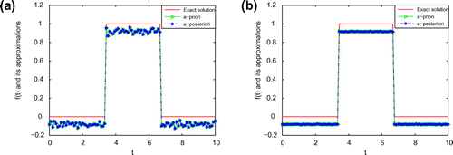
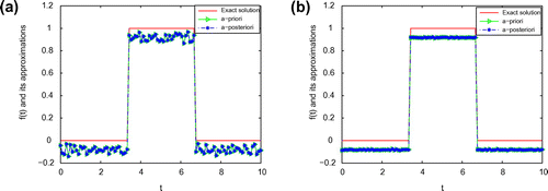
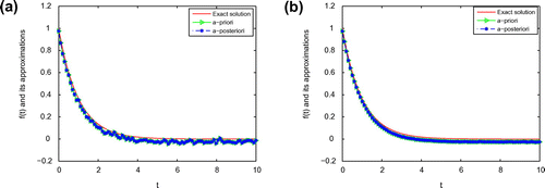
[32]Consider the following discontinuous case:5.12 $$\begin{array}{c}\hfill f(t)=\left\{\begin{array}{cc}0,\hfill & 0\le t\le 10/3,\hfill \\ 1,\hfill & 10/3<t\le 20/3,\hfill \\ 0,\hfill & 20/3<t\le 10.\hfill \end{array}\right.\end{array}$$5.12 From Figures 1–9, we can find that the smaller $\mathit{\epsilon }$, the better the computed approximation is, and the smaller the $\mathit{\alpha }$ is, the better the computed approximation is. Moreover, we can also easily find that a posteriori parameter choice also works well. From Figures 4–9, it can be seen that the numerical solution is less ideal than that of Example 1. It is not difficult to see that the well-known Gibbs phenomenon and the recovered data near the non-smooth and discontinuities points are not accurate. Taking into consideration of the ill-posedness of the problem, the results presented in Figures 4–9 are reasonable.

Figure 1. The comparison of the numerical effects between the exact solution and its computed approximations for $p=1$, $\mathit{\alpha }=0.1$ with Example 1: (a) $\mathit{\epsilon }=0.01$, (b) $\mathit{\epsilon }=0.001$.

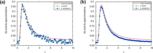
Figure 2. The comparison of the numerical effects between the exact solution and its computed approximations for $p=1$, $\mathit{\alpha }=0.3$ with Example 1: (a) $\mathit{\epsilon }=0.01$, (b) $\mathit{\epsilon }=0.001$.

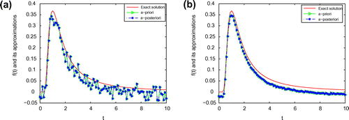
Figure 3. The comparison of the numerical effects between the exact solution and its computed approximations for $p=1$, $\mathit{\alpha }=0.6$ with Example 1: (a) $\mathit{\epsilon }=0.01$, (b) $\mathit{\epsilon }=0.001$.

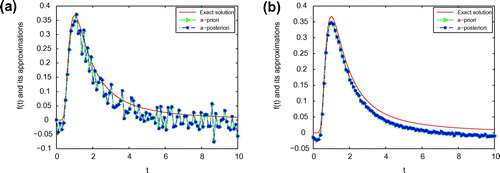
Figure 4. The comparison of the numerical effects between the exact solution and its computed approximations for $p=1$, $\mathit{\alpha }=0.1$ with Example 2: (a) $\mathit{\epsilon }=0.01$, (b) $\mathit{\epsilon }=0.001$.

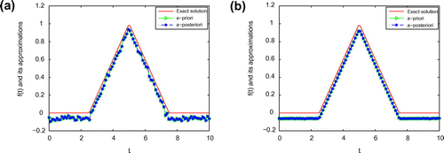
Figure 5. The comparison of the numerical effects between the exact solution and its computed approximations for $p=1$, $\mathit{\alpha }=0.3$ with Example 2: (a) $\mathit{\epsilon }=0.01$, (b) $\mathit{\epsilon }=0.001$.

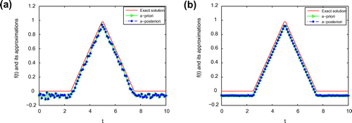
Figure 6. The comparison of the numerical effects between the exact solution and its computed approximations for $p=1$, $\mathit{\alpha }=0.6$ with Example 2: (a) $\mathit{\epsilon }=0.01$, (b) $\mathit{\epsilon }=0.001$.

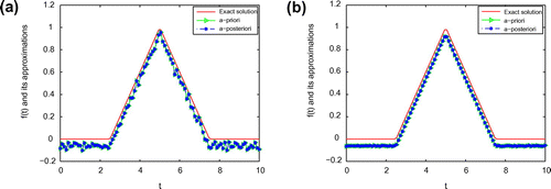
Figure 7. The comparison of the numerical effects between the exact solution and its computed approximations for $p=1$, $\mathit{\alpha }=0.1$ with Example 3: (a) $\mathit{\epsilon }=0.01$, (b) $\mathit{\epsilon }=0.001$.

Figure 8. The comparison of the numerical effects between the exact solution and its computed approximations for $p=1$, $\mathit{\alpha }=0.3$ with Example 3: (a) $\mathit{\epsilon }=0.01$, (b) $\mathit{\epsilon }=0.001$.

Figure 9. The comparison of the numerical effects between the exact solution and its computed approximations for $p=1$, $\mathit{\alpha }=0.6$ with Example 3: (a) $\mathit{\epsilon }=0.01$, (b) $\mathit{\epsilon }=0.001$.

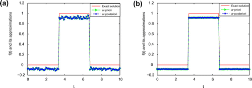
6 Identifying the unknown source of separable variables

In this section, we will use the Fourier regularization method to identify the unknown source of separable variables in the following time-fractional diffusion equation:6.1 $$\begin{array}{c}\hfill \left\{\begin{array}{cc}{\mathit{\partial }}_{0^{+}}^{\mathit{\alpha }}u(x,t)-u_{xx}(x,t)=\mathit{\lambda }(x)f(t),\hfill & x>0,t>0,\hfill \\ u(x,0)=0,\hfill & x\ge 0,\hfill \\ u(0,t)=0,\hfill & t\ge 0,\hfill \\ {u(x,t)|}_{x\to \infty }\text{bounded},\hfill & t\ge 0,\hfill \\ u(1,t)=g(t),\hfill & t\ge 0,\hfill \end{array}\right.\end{array}$$6.1 where $\mathit{\lambda }(x)f(t)$ denotes the source (sink) term. We assume the space-dependent source term $\mathit{\lambda }(x)$ is known and satisfied6.2 $$\begin{array}{c}\hfill \mathit{\lambda }(x)\in C[0,+\infty ),0<p_0\le \mathit{\lambda }(x)\le q_0.\end{array}$$6.2 The time-dependent source term $f(t)$ is unknown. Our purpose is to identify $f(t)$ from the additional data $u(1,t)=g(t)$.

Using the Fourier transform, we obtain the solution of the problem (6.16.1 $$\begin{array}{c}\hfill \left\{\begin{array}{cc}{\mathit{\partial }}_{0^{+}}^{\mathit{\alpha }}u(x,t)-u_{xx}(x,t)=\mathit{\lambda }(x)f(t),\hfill & x>0,t>0,\hfill \\ u(x,0)=0,\hfill & x\ge 0,\hfill \\ u(0,t)=0,\hfill & t\ge 0,\hfill \\ {u(x,t)|}_{x\to \infty }\text{bounded},\hfill & t\ge 0,\hfill \\ u(1,t)=g(t),\hfill & t\ge 0,\hfill \end{array}\right.\end{array}$$6.1 ) in frequency space as follows:6.3 $$\begin{array}{c}\hfill \widehat{f}(\mathit{\xi })=\frac{{(i\mathit{\xi })}^{\frac{\mathit{\alpha }}{2}}}{{\int }_0^1\mathit{\lambda }(\mathit{\tau })sinh({(i\mathit{\xi })}^{\frac{\mathit{\alpha }}{2}}(\mathit{\tau }-1))d\mathit{\tau }}\widehat{g}(\mathit{\xi }).\end{array}$$6.3 So6.4 $$\begin{array}{c}\hfill f(t)=\frac{1}{\sqrt{2\mathit{\pi }}}{\int }_{-\infty }^{\infty }{e}^{i\mathit{\xi }t}\frac{{(i\mathit{\xi })}^{\frac{\mathit{\alpha }}{2}}}{{\int }_0^1\mathit{\lambda }(\mathit{\tau })sinh({(i\mathit{\xi })}^{\frac{\mathit{\alpha }}{2}}(\mathit{\tau }-1))d\mathit{\tau }}\widehat{g}(\mathit{\xi }).\end{array}$$6.4 Using the Fourier regularization method, we give the Fourier regularization solution of problem (6.16.1 $$\begin{array}{c}\hfill \left\{\begin{array}{cc}{\mathit{\partial }}_{0^{+}}^{\mathit{\alpha }}u(x,t)-u_{xx}(x,t)=\mathit{\lambda }(x)f(t),\hfill & x>0,t>0,\hfill \\ u(x,0)=0,\hfill & x\ge 0,\hfill \\ u(0,t)=0,\hfill & t\ge 0,\hfill \\ {u(x,t)|}_{x\to \infty }\text{bounded},\hfill & t\ge 0,\hfill \\ u(1,t)=g(t),\hfill & t\ge 0,\hfill \end{array}\right.\end{array}$$6.1 ) for noisy data $g^{\mathit{\delta }}(t)$ as follows:6.5 $$\begin{array}{c}\hfill f_{{\mathit{\eta }}_{max}}^{\mathit{\delta }}(t):=\frac{1}{\sqrt{2\mathit{\pi }}}{\int }_{-\infty }^{\infty }{e}^{i\mathit{\xi }t}\frac{{(i\mathit{\xi })}^{\frac{\mathit{\alpha }}{2}}}{{\int }_0^1\mathit{\lambda }(\mathit{\tau })sinh({(i\mathit{\xi })}^{\frac{\mathit{\alpha }}{2}}(\mathit{\tau }-1))d\mathit{\tau }}{\widehat{g}}^{\mathit{\delta }}(\mathit{\xi }){\mathit{\chi }}_{max}d\mathit{\xi },\end{array}$$6.5 where ${\mathit{\chi }}_{max}$ is the characteristic function of the interval $[-{\mathit{\eta }}_{max},{\mathit{\eta }}_{max}]$, i.e.6.6 $$\begin{array}{c}\hfill {\mathit{\chi }}_{max}(\mathit{\xi })=\left\{\begin{array}{cc}1,\hfill & |\mathit{\xi }|\le {\mathit{\eta }}_{max},\hfill \\ 0,\hfill & |\mathit{\xi }|>{\mathit{\eta }}_{max},\hfill \end{array}\right.\end{array}$$6.6 and ${\mathit{\eta }}_{max}$ is a constant which will be selected appropriately as regularization parameter.

6.1 A priori choice rule

Theorem 6.1.1

Let $f(t)$ given by (6.46.4 $$\begin{array}{c}\hfill f(t)=\frac{1}{\sqrt{2\mathit{\pi }}}{\int }_{-\infty }^{\infty }{e}^{i\mathit{\xi }t}\frac{{(i\mathit{\xi })}^{\frac{\mathit{\alpha }}{2}}}{{\int }_0^1\mathit{\lambda }(\mathit{\tau })sinh({(i\mathit{\xi })}^{\frac{\mathit{\alpha }}{2}}(\mathit{\tau }-1))d\mathit{\tau }}\widehat{g}(\mathit{\xi }).\end{array}$$6.4 ) be the exact solution of (6.16.1 $$\begin{array}{c}\hfill \left\{\begin{array}{cc}{\mathit{\partial }}_{0^{+}}^{\mathit{\alpha }}u(x,t)-u_{xx}(x,t)=\mathit{\lambda }(x)f(t),\hfill & x>0,t>0,\hfill \\ u(x,0)=0,\hfill & x\ge 0,\hfill \\ u(0,t)=0,\hfill & t\ge 0,\hfill \\ {u(x,t)|}_{x\to \infty }\text{bounded},\hfill & t\ge 0,\hfill \\ u(1,t)=g(t),\hfill & t\ge 0,\hfill \end{array}\right.\end{array}$$6.1 ) and $f_{{\mathit{\eta }}_{max}}^{\mathit{\delta }}(t)$ be the Fourier regularization solution given by (6.56.5 $$\begin{array}{c}\hfill f_{{\mathit{\eta }}_{max}}^{\mathit{\delta }}(t):=\frac{1}{\sqrt{2\mathit{\pi }}}{\int }_{-\infty }^{\infty }{e}^{i\mathit{\xi }t}\frac{{(i\mathit{\xi })}^{\frac{\mathit{\alpha }}{2}}}{{\int }_0^1\mathit{\lambda }(\mathit{\tau })sinh({(i\mathit{\xi })}^{\frac{\mathit{\alpha }}{2}}(\mathit{\tau }-1))d\mathit{\tau }}{\widehat{g}}^{\mathit{\delta }}(\mathit{\xi }){\mathit{\chi }}_{max}d\mathit{\xi },\end{array}$$6.5 ). Let assumptions (1.21.2 $$\begin{array}{cc}\hfill {\mathit{\partial }}_{0^{+}}^{\mathit{\alpha }}u(x,t)& =\frac{1}{\mathrm{\Gamma }(1-\mathit{\alpha })}{\int }_0^t\frac{\mathit{\partial }u(x,s)}{\mathit{\partial }s}\frac{ds}{{(t-s)}^{\mathit{\alpha }}},0<\mathit{\alpha }<1,\hfill \end{array}$$1.2 ) and priori condition (1.101.10 $$\begin{array}{c}\hfill {\Vert f(·)\Vert }_p\le E,p>0,\end{array}$$1.10 ) hold. If we select6.7 $$\begin{array}{c}\hfill {\mathit{\eta }}_{max}={\left(\frac{E}{\mathit{\delta }}\right)}^{\frac{1}{p+\mathit{\alpha }}},\end{array}$$6.7 then we obtain the following estimate:6.8 $$\begin{array}{c}\hfill \Vert f(·)-f_{{\mathit{\eta }}_{max}}^{\mathit{\delta }}(·)\Vert \le \frac{p_0+2}{p_0}{\mathit{\delta }}^{\frac{p}{p+\mathit{\alpha }}}{E}^{\frac{\mathit{\alpha }}{p+\mathit{\alpha }}}(1+o(1)),as\mathit{\delta }\to 0.\end{array}$$6.8

Proof

Using the Parseval formula and the triangle inequality, we know$$\begin{array}{cc}& {\displaystyle \Vert f(·)-f_{{\mathit{\eta }}_{max}}^{\mathit{\delta }}(·)\Vert =\Vert \widehat{f}(·)-{\widehat{f}}_{{\mathit{\eta }}_{max}}^{\mathit{\delta }}(·)\Vert }\hfill \\ \hfill {\displaystyle }& =∥\frac{{(i\mathit{\xi })}^{\frac{\mathit{\alpha }}{2}}}{{\int }_0^1\mathit{\lambda }(\mathit{\tau })sinh({(i\mathit{\xi })}^{\frac{\mathit{\alpha }}{2}}(\mathit{\tau }-1))d\mathit{\tau }},\widehat{g},(\mathit{\xi }),-,\frac{{(i\mathit{\xi })}^{\frac{\mathit{\alpha }}{2}}}{{\int }_0^1\mathit{\lambda }(\mathit{\tau })sinh({(i\mathit{\xi })}^{\frac{\mathit{\alpha }}{2}}(\mathit{\tau }-1))d\mathit{\tau }},{\widehat{g}}^{\mathit{\delta }},(\mathit{\xi }),{\mathit{\chi }}_{max}∥\hfill \\ \hfill {\displaystyle }& \le ∥\frac{{(i\mathit{\xi })}^{\frac{\mathit{\alpha }}{2}}}{{\int }_0^1\mathit{\lambda }(\mathit{\tau })sinh({(i\mathit{\xi })}^{\frac{\mathit{\alpha }}{2}}(\mathit{\tau }-1))d\mathit{\tau }},\widehat{g},(\mathit{\xi }),-,\frac{{(i\mathit{\xi })}^{\frac{\mathit{\alpha }}{2}}}{{\int }_0^1\mathit{\lambda }(\mathit{\tau })sinh({(i\mathit{\xi })}^{\frac{\mathit{\alpha }}{2}}(\mathit{\tau }-1))d\mathit{\tau }},\widehat{g},(\mathit{\xi }),{\mathit{\chi }}_{max}∥\hfill \\ \hfill {\displaystyle }& +∥\frac{{(i\mathit{\xi })}^{\frac{\mathit{\alpha }}{2}}}{{\int }_0^1\mathit{\lambda }(\mathit{\tau })sinh({(i\mathit{\xi })}^{\frac{\mathit{\alpha }}{2}}(\mathit{\tau }-1))d\mathit{\tau }},\widehat{g},(\mathit{\xi }),{\mathit{\chi }}_{max}\hfill \\ \hfill & -,\frac{{(i\mathit{\xi })}^{\frac{\mathit{\alpha }}{2}}}{{\int }_0^1\mathit{\lambda }(\mathit{\tau })sinh({(i\mathit{\xi })}^{\frac{\mathit{\alpha }}{2}}(\mathit{\tau }-1))d\mathit{\tau }},{\widehat{g}}^{\mathit{\delta }},(\mathit{\xi }),{\mathit{\chi }}_{max}∥\hfill \\ \hfill {\displaystyle }& =∥\frac{{(i\mathit{\xi })}^{\frac{\mathit{\alpha }}{2}}}{{\int }_0^1\mathit{\lambda }(\mathit{\tau })sinh({(i\mathit{\xi })}^{\frac{\mathit{\alpha }}{2}}(\mathit{\tau }-1))d\mathit{\tau }},\widehat{g},(\mathit{\xi }),(1-{\mathit{\chi }}_{max})∥\hfill \\ \hfill & +∥\frac{{(i\mathit{\xi })}^{\frac{\mathit{\alpha }}{2}}}{{\int }_0^1\mathit{\lambda }(\mathit{\tau })sinh({(i\mathit{\xi })}^{\frac{\mathit{\alpha }}{2}}(\mathit{\tau }-1))d\mathit{\tau }},(\widehat{g}(\mathit{\xi })-{\widehat{g}}^{\mathit{\delta }}(\mathit{\xi })),{\mathit{\chi }}_{max}∥\hfill \\ \hfill {\displaystyle }& ={\left(\underset{|\mathit{\xi }|>{\mathit{\eta }}_{max}}{\int },{\left(\frac{{(i\mathit{\xi })}^{\frac{\mathit{\alpha }}{2}}}{{\int }_0^1\mathit{\lambda }(\mathit{\tau })sinh({(i\mathit{\xi })}^{\frac{\mathit{\alpha }}{2}}(\mathit{\tau }-1))d\mathit{\tau }},\widehat{g},(\mathit{\xi })\right)}^2,d,\mathit{\xi }\right)}^{\frac{1}{2}}\hfill \\ \hfill {\displaystyle }& +{\left(\underset{|\mathit{\xi }|\le {\mathit{\eta }}_{max}}{\int },{\left(\frac{{(i\mathit{\xi })}^{\frac{\mathit{\alpha }}{2}}}{{\int }_0^1\mathit{\lambda }(\mathit{\tau })sinh({(i\mathit{\xi })}^{\frac{\mathit{\alpha }}{2}}(\mathit{\tau }-1))d\mathit{\tau }},(\widehat{g}(\mathit{\xi })-{\widehat{g}}^{\mathit{\delta }}(\mathit{\xi }))\right)}^2,d,\mathit{\xi }\right)}^{\frac{1}{2}}\hfill \\ \hfill {\displaystyle }& \le {\left(\underset{|\mathit{\xi }|>{\mathit{\eta }}_{max}}{\int },{\left(\widehat{f},(\mathit{\xi }),{(1+{\mathit{\xi }}^2)}^{\frac{p}{2}},{(1+{\mathit{\xi }}^2)}^{-\frac{p}{2}}\right)}^2,d,\mathit{\xi }\right)}^{\frac{1}{2}}\hfill \\ \hfill {\displaystyle }& +\underset{|\mathit{\xi }|\le {\mathit{\eta }}_{max}}{sup}\left|\frac{{(i\mathit{\xi })}^{\frac{\mathit{\alpha }}{2}}}{{\int }_0^1\mathit{\lambda }(\mathit{\tau })sinh({(i\mathit{\xi })}^{\frac{\mathit{\alpha }}{2}}(\mathit{\tau }-1))d\mathit{\tau }}\right|{\left(\underset{|\mathit{\xi }|\le {\mathit{\eta }}_{max}}{\int },{(\widehat{g}(\mathit{\xi })-{\widehat{g}}^{\mathit{\delta }}(\mathit{\xi }))}^2,d,\mathit{\xi }\right)}^{\frac{1}{2}}\hfill \\ \hfill {\displaystyle }& \le \underset{|\mathit{\xi }|>{\mathit{\eta }}_{max}}{sup}{(1+{\mathit{\xi }}^2)}^{-\frac{p}{2}}{\left(\underset{|\mathit{\xi }|>{\mathit{\eta }}_{max}}{\int },{(\widehat{f}(\mathit{\xi }){(1+{\mathit{\xi }}^2)}^{\frac{p}{2}})}^2,d,\mathit{\xi }\right)}^{\frac{1}{2}}\hfill \\ \hfill & +\underset{|\mathit{\xi }|\le {\mathit{\eta }}_{max}}{sup}\left|\frac{{(i\mathit{\xi })}^{\frac{\mathit{\alpha }}{2}}}{p_0{\int }_0^{1}sinh({(i\mathit{\xi })}^{\frac{\mathit{\alpha }}{2}}(\mathit{\tau }-1))d\mathit{\tau }}\right|\mathit{\delta }.\hfill \\ \hfill {\displaystyle }& \le \frac{1}{{\mathit{\eta }}_{max}^p}E+\underset{|\mathit{\xi }|\le {\mathit{\eta }}_{max}}{sup}\left|\frac{{(i\mathit{\xi })}^{\mathit{\alpha }}}{p_0(1-cosh({(i\mathit{\xi })}^{\frac{\mathit{\alpha }}{2}})},)\right|\mathit{\delta }\hfill \\ \hfill {\displaystyle }& \le \frac{1}{{\mathit{\eta }}_{max}^p}E+\underset{|\mathit{\xi }|\le {\mathit{\eta }}_{max}}{sup}\left(\frac{{|\mathit{\xi }|}^{\mathit{\alpha }}}{p_0(1-e^{-{|\mathit{\xi }|}^{\frac{\mathit{\alpha }}{2}}cos(\frac{\mathit{\pi }}{4}\mathit{\alpha })})}\right)\mathit{\delta }\hfill \\ \hfill {\displaystyle }& \le \frac{1}{{\mathit{\eta }}_{max}^p}E+\frac{2}{p_0}{\mathit{\eta }}_{max}^{\mathit{\alpha }}\mathit{\delta }+\frac{2}{p_0{(cos(\frac{\mathit{\pi }}{4}\mathit{\alpha }))}^2}\mathit{\delta }\hfill \\ \hfill {\displaystyle }& =\frac{p_0+2}{p_0}{\mathit{\delta }}^{\frac{p}{p+\mathit{\alpha }}}{E}^{\frac{\mathit{\alpha }}{p+\mathit{\alpha }}}+\frac{2}{p_0{(cos(\frac{\mathit{\pi }}{4}\mathit{\alpha }))}^2}\mathit{\delta }\hfill \\ \hfill {\displaystyle }& =\frac{p_0+2}{p_0}{\mathit{\delta }}^{\frac{p}{p+\mathit{\alpha }}}{E}^{\frac{\mathit{\alpha }}{p+\mathit{\alpha }}}(1+o(1)),as\mathit{\delta }\to 0.\hfill \end{array}$$$\square$

6.2 The a posteriori choice rule

In this section, we consider the a posteriori regularization parameter choice rule. Choose the regularization parameter ${\mathit{\eta }}_{max}$ as the solution of the equation6.9 $$\begin{array}{c}\hfill \Vert (1-{\mathit{\chi }}_{max}(\mathit{\xi })){\widehat{g}}^{\mathit{\delta }}(\mathit{\xi })\Vert =\mathit{\tau }\mathit{\delta },\mathit{\tau }>1\mathrm{is}\mathrm{a}\mathrm{constant},\end{array}$$6.9 where ${\mathit{\chi }}_{max}(\mathit{\xi })$ is defined by (6.66.6 $$\begin{array}{c}\hfill {\mathit{\chi }}_{max}(\mathit{\xi })=\left\{\begin{array}{cc}1,\hfill & |\mathit{\xi }|\le {\mathit{\eta }}_{max},\hfill \\ 0,\hfill & |\mathit{\xi }|>{\mathit{\eta }}_{max},\hfill \end{array}\right.\end{array}$$6.6 ).

In order to obtain the error estimate for the a posteriori choice rule of the regularization parameter, we need the following lemmas:

Lemma 6.2.1

If ${\mathit{\eta }}_{max}$ is the solution of Equation (6.96.9 $$\begin{array}{c}\hfill \Vert (1-{\mathit{\chi }}_{max}(\mathit{\xi })){\widehat{g}}^{\mathit{\delta }}(\mathit{\xi })\Vert =\mathit{\tau }\mathit{\delta },\mathit{\tau }>1\mathrm{is}\mathrm{a}\mathrm{constant},\end{array}$$6.9 ), then we obtain the following inequality hold:6.10 $$\begin{array}{c}\hfill |{\mathit{\eta }}_{max}|\le {\left(\frac{2q_{0}E}{(\mathit{\tau }-1)\mathit{\delta }}\right)}^{\frac{1}{p+\mathit{\alpha }}}.\end{array}$$6.10

Proof

The proof of Lemma 6.2.1 is similar to the proof of Lemma 4.2.3, we omit it.$\square$

Lemma 6.2.2

If ${\mathit{\eta }}_{max}$ is the solution of Equation (6.96.9 $$\begin{array}{c}\hfill \Vert (1-{\mathit{\chi }}_{max}(\mathit{\xi })){\widehat{g}}^{\mathit{\delta }}(\mathit{\xi })\Vert =\mathit{\tau }\mathit{\delta },\mathit{\tau }>1\mathrm{is}\mathrm{a}\mathrm{constant},\end{array}$$6.9 ), then we also get the following inequality:6.11 $$\begin{array}{c}\hfill \Vert (1-{\mathit{\chi }}_{max}(\mathit{\xi }))\widehat{g}(\mathit{\xi })\Vert \le (\mathit{\tau }+1)\mathit{\delta }.\end{array}$$6.11

Proof

The proof of Lemma 6.2.2 is similar to the proof of Lemma 4.2.4, we omit it $\square$

Now we give the main result of this section.

Theorem 6.2.3

Assume the conditions (1.41.4 $$\begin{array}{c}\hfill \Vert g-g^{\mathit{\delta }}\Vert \le \mathit{\delta },\end{array}$$1.4 ) and (1.101.10 $$\begin{array}{c}\hfill {\Vert f(·)\Vert }_p\le E,p>0,\end{array}$$1.10 ) hold and take the solution ${\mathit{\eta }}_{max}$ of Equation (6.96.9 $$\begin{array}{c}\hfill \Vert (1-{\mathit{\chi }}_{max}(\mathit{\xi })){\widehat{g}}^{\mathit{\delta }}(\mathit{\xi })\Vert =\mathit{\tau }\mathit{\delta },\mathit{\tau }>1\mathrm{is}\mathrm{a}\mathrm{constant},\end{array}$$6.9 ) as the regularization parameter, then there holds the following error estimate:6.12 $$\begin{array}{cc}& \Vert f(·)-f_{{\mathit{\eta }}_{max}}^{\mathit{\delta }}(·)\Vert \hfill \\ \hfill & \le \left({\left(\frac{2}{p_0},(\mathit{\tau }+1)\right)}^{\frac{p}{p+\mathit{\alpha }}},+,\frac{2}{p_0},{(\frac{2q_0}{\mathit{\tau }-1})}^{\frac{\mathit{\alpha }}{p+\mathit{\alpha }}}\right)E^{\frac{\mathit{\alpha }}{p+\mathit{\alpha }}}{\mathit{\delta }}^{\frac{p}{p+\mathit{\alpha }}}(1+o(1)),as\mathit{\delta }\to 0.\hfill \end{array}$$6.12

Proof

The proof of Theorem 6.2.3 is similar to the proof of Theorem 4.2.5, we omit it.$\square$

6.3 Numerical example

In this section, we choose an example to show the effectiveness and stability of our proposed method.

Example 4

Take a source function $\mathit{\lambda }(x)=1+sinx$ and $f(t)=e^{-t}$.

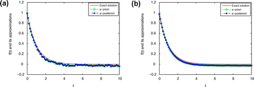
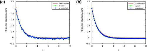
From Figures 10–12, we can also find that the smaller $\mathit{\epsilon }$, the better the computed approximation is, and the smaller the $\mathit{\alpha }$ is, the better the computed approximation is. Meanwhile, we can easily find that a posteriori parameter choice also works well. So, the Fourier regularization method is very effective for identifying the unknown source which is separable variable.

Figure 10. The comparison of the numerical effects between the exact solution and its computed approximations for $p=1$, $\mathit{\alpha }=0.1$ with Example 4: (a) $\mathit{\epsilon }=0.01$, (b) $\mathit{\epsilon }=0.001$.

Figure 11. The comparison of the numerical effects between the exact solution and its computed approximations for $p=1$, $\mathit{\alpha }=0.3$ with Example 4: (a) $\mathit{\epsilon }=0.01$, (b) $\mathit{\epsilon }=0.001$.

Figure 12. The comparison of the numerical effects between the exact solution and its computed approximations for $p=1$, $\mathit{\alpha }=0.6$ with Example 4: (a) $\mathit{\epsilon }=0.01$, (b) $\mathit{\epsilon }=0.001$.

7 Conclusions

In this paper, the Fourier regularization method is used to identify the unknown source term which depends only on the time variable or is separable variable for the time-fractional diffusion equation. Under the a priori condition, we gave the optimal error bound for this problem. Moreover, we obtained the stability estimate using the conditional stability. Thirdly, for the a priori and the a posteriori parameter choice rules, we all obtain the Höder type error estimates which are all order-optimal. Finally, the numerical experiments show the proposed methods work effectively.

Notes

The project is supported by the National Natural Science Foundation of China (No.11171136, No.11261032), the Distinguished Young Scholars Fund of Lan Zhou University of Technology (Q201015), the basic scientific research business expenses of Gansu province college and the Natural Science Foundation of Gansu province (1310RJYA021).

References

- Metzler R, Klafter J. The random walk’s guide to anomalous diffusion: a fractional dynamics approach. Phys. Rep. 2000;339:1–77.
- Podlubny I. Fractional differential equations: an introduction to fractional derivatives. Fractional differential equations, to methods of their solution and some of their applications (mathematics in science and engineering vol 198). San Diego (CA): Academic; 1999.
- Scalas E, Gorenflo R, Mainardi F. Fractional calculus and continuous-time finance. Phys. A. 2000;284:376–384.
- Su L, Wang W, Xu Q. Finite difference methods for fractional dispersion equations. Appl. Math. Comput. 2010;216:3329–3334.
- Miller KS, Ross B. An introduction to the fractional calculus and fractional differential equations. New York (NY): Wiley; 1993.
- Oldham KB, Spanier J. The fractional calculus. New York (NY): Academic Press; 1974.
- Sokolov IM, Klafter J. From diffusion to anomalous diffusion: a century after Einsteins Brownian motion. Chaos. 2005;15:1–7.
- Cheng J, Nakagawa J, Yamamoto M, Yamazaki T. Uniqueness in an inverse problem for a one-dimensional fractional diffusion equation. Inverse Prob. 2009;25:115002.
- Adams EE, Gelhar LW. Field study of dispersion in a heterogeneous aquifer 2. Spatial moments analysis. Water Resour. Res. 1992;28:3293–3307.
- Zhou L, Selim HM. Application of the fractional advection-dispersion equations in porous media. Soli. Sci. Soc. Am. J. 2003;67:1079–1084.
- Berkowitz B, Scher H, Silliman SE. Anomalous transport in laboratory-scale, heterogeneous porus media. Water Resour. Res. 2000;36:149–158.
- Hatano Y, Hatano N. Dispersive transport of ions in column experiments: an explanation of long-tailed profiles. Water Resour. Res. 1998;34:1027–1033.
- Jiang Y, Ma J. High-order finite element methods for time-fractional partial differential equations. J. Comput. Appl. Math. 2011;235:3285–3290.
- Lin YM, Xu CJ. Finite difference/spectral approximations for the time-fractional diffusion equation. J. Comput. Phys. 2007;225:1533–1552.
- Luchko Y. Some uniqueness and existence results for the initial-boundary-value problems for the generalized time-fractional diffusion equation. Comput. Math. Appl. 2010;59:1766–1772.
- Luchko Y. Maximum principle and its application for the time-fractional diffusion equations. Fract. Calc. Appl. Anal. 2011;14:110–124.
- Murio DA. Implicit finite difference approximation for time fractional diffusion equations. Comput. Math. Appl. 2008;56:1138–1145.
- Zhang P, Liu F. Implicit difference approximation for the time fractional diffusion equation. J. Appl. Math. Comput. 2006;22:87–99.
- Xiong XT, Wang JX, Li M. An optimal method for fractional heat conduction problem backward in time. Appl. Anal. 2012;91:823–840.
- Ahmadabadi MN, Arab M, Malek Ghaini FM. The method of fundamental solutions for the inverse space-dependent heat source problem. Eng. Anal. Bound. Elem. 2009;33:1231–1235.
- Cannon JR, Duchateau P. Structural identification of an unknown source term in a heat equation. Inverse Prob. 1998;14:535–551.
- Farcas A, Lesnic D. The boundary-element method for the determination of a heat source dependent on one variable. J. Eng. Math. 2006;54:375–388.
- Li GS. Data compatibility and conditional stability for an inverse source problem in the heat equation. Appl. Math. Comput. 2006;173:566–581.
- Liu FB. A modified genetic algorithm for solving the inverse heat transfer problem of estimating plan heat source. Int. J. Heat Mass Transfer. 2008;51:3745–3752.
- Liu CH. A two-stage LGSM to identify time-dependent heat source through an internal measurement of temperature. Int. J. Heat Mass Transfer. 2009;52:1635–1642.
- Yan L, Yang FL, Fu CL. A meshless method for solving an inverse spacewise-dependent heat source problem. J. Comput. Phys. 2009;228:123–136.
- Yang F, Fu CL. The method of simplified Tikhonov regularization for dealing with the inverse time-dependent heat source problem. Comput. Math. Appl. 2010;60:1228–1236.
- Yamamoto M. Conditional stability in determination of force terms of heat equations in a rectangle. Math. Comput. Modell. 1993;18:79–88.
- Zhang Y, Xu X. Inverse source problem for a fractional diffusion equation. Inverse Prob. 2011;27:035010 (12pp).
- Wei H, Chen W, Sun HG, Li XC. A coupled method for inverse source problem of spatial fractional anonmalous diffusion equations. Inverse Probl. Sci. Eng. 2010;18:945–956.
- Chi GS, Li GS, Jia XZ. Numerical inversions of a source term in the FADE with a Dirichlet boundary condition using final observations. Comput. Math. Appl. 2011;62:1619–1626.
- Wei T, Zhang ZQ. Reconstruction of a time-dependent source term in a time-fractional diffusion equation. Eng. Anal. Bound. Elem. 2013;37:23–31.
- Tian WY, Li C, Deng WH, Wu YJ. Regularization methods for unknown source in space fractional diffusion equation. Math. Comput. Simulat. 2012;85:45–56.
- Fu P, Fu CL, Xiong XT, Li HF. Two regularization methods and the order optimal error estimates for a sideways parabolic equation. Comput. Math. Appl. 2005;49:777–788.
- Qian Z, Fu CL. Regularization strategies for a two-dimensional inverse heat conduction problem. Inverse Prob. 2007;23:1053–1068.
- Xiong XT, Fu CL, Li HF. Fourier regularization method of a sideways heat equation for determining surface heat flux. J. Math. Anal. Appl. 2006;317:331–348.
- Fu CL, Feng XL, Qian Z. The Fourier regularization for solving the Cauchy problem for the Helmholtz equation. Appl. Numer. Math. 2009;59:2625–2640.
- Fu CL, Li HF, Qian Z, Xiong XT. Fourier regularization method for solving a Cauchy problem for the Laplace equation. Inverse Prob. Sci. Eng. 2008;16:159–169.
- Regińska T, Regiński K. Approximate solution of a Cauchy problem for the Helmholtz equation. Inverse Prob. 2008;22:975–989.
- Fu CL, Xiong XT, Qian Z. Fourier regularization for a backward heat equation. J. Math. Anal. Appl. 2007;331:472–480.
- Qian Z, Fu CL, Xiong XT, Fu P. Fourier regularization method for solving the surface heat flux from interior observations. Math. Comput. Model. 2005;42:489–498.
- Fu CL, Dou FF, Feng XL, Qian Z. A simple regularization method for stable analytic continuation. Inverse Prob. 2008;24:065003.
- Dou FF, Fu CL, Yang FL. Optimal error bound and Fourier regularization for identifying an unknown source in the heat equation. J. Comput. Appl. Math. 2008;230:728–737.
- Yang F, Fu CL. Two regularization methods to identify time-dependent heat source through an internal measurement of temperature. Math. Comput. Model. 2011;53:793–804.
- Ivanchov MI. The inverse problem of determining the heat source power for a parabolic equation under arbitrary boundary conditions. J. Math. Sci. 1998;88:432–436.
- Schröer T, Tautenhahn U. On the ‘optimal’ regularization methods for solving linear ill-posed problems. Z. Anal. Anwend. 1994;13:697–710.
- Tautenhahn U. Optimal stable approximations for the sideways heat equation. J. Inverse Ill-Posed Probl. 1997;5:287–307.
- Tautenhahn U. Optimality for ill-posed problems under general source conditions. Numer. Funct. Anal. Optim. 1998;19:377–398.
- Vainikko G. On the optimality of methods for ill-posed problems. Z. Anal. Anwend. 1987;64:351–362.
- Tautenhahn U, Gorenflo R. On optimal regularization methods for fractional differentiation. J. Anal. Appl. 1999;18:449–467.
- Eldén L, Berntsson F, Regińska T. Wavelet and Fourier methods for solving the sideways heat equation. SIAM J. Sci. Comput. 2000;21:2187–2205.