Coupled SelfSim and genetic programming for non-linear material constitutive modelling

Abstract

In the present study, an improved SelfSim is combined with a recent genetic programming technique called linear GP (LGP) for the inverse extraction of non-linear material behaviour. The SelfSim prepares a comprehensive database including stresses and strains of the structural elements. Then, a steady-state LGP is used to formulate the strain–stress relationship. In this research, a space truss with a reference material model is used as a hypothetical structure. The derived LGP-based formula is very simple and can be employed for design and pre-design purposes. The implementation of LGP-based model is also tested in a general purpose finite element programme. Since the proposed model is an explicit formula, its implementation becomes standard and practically useful. The results show that the procedure is reliable and can be used to derive and formulate the non-linear constitutive material models with a high degree of accuracy.

Keywords:

• inverse analysis
• artificial neural network
• genetic programming
• non-linear material constitutive model
• linear genetic programming

1. Introduction

Recently, numerical methods have been widely employed to predict the complex material behaviour and it has been an important research topic in the field of computational mechanics. Strain–strain relationship is a key factor in engineering design and especially in structural design.[1] Loading history and material responses, obtained from the experiments, are required to estimate the model parameters. One of the main issues is that the material response subjected to different loadings are physically different.[2] Another problem is that the laboratory material tests, such as biaxial or triaxial tests, have additional uncertainties in model-based predictions.[3]

Metaheuristics, such as artificial neural networks (ANNs), have been widely used in the last two decades for engineering modelling [4] and also constitutive material modelling.[5,6] One of the heuristic methods for constitutive material modelling was proposed by Ghaboussi et al. [7]. The idea called auto-progressive training method can automatically train an ANN-based material constitutive model using only global load–deflection response measured in a structural test. This method is an online training method for the multi-layer perceptron neural network for constitutive material modelling and predicts stress–strain behaviour of materials. An interesting feature of the auto-progressive training is that it can self-train the neural network model by pre-training the neural network model with linear elastic behaviour and limiting the number of training epochs (e.g. 100) during auto-progressive cycles. This helps to avoid premature training while learning non-linear behaviour of materials. The auto-progressive training of the neural network can also be protected against both overfitting and underfitting by changing the number of finite elements under post-processing or the number of load steps. There are some other methods in the literature in which genetic algorithm (GA)-based multi-objective optimization is used to find a family of optimum neural networks (e.g. [8,9]), but the main advantage of the auto-progressive training method is that it is very fast and does not need any optimization algorithm.

Yun et al. [10,11] recently improved the SelfSim method for non-uniform, non-linear and inelastic material modelling. Advantages of the ANN-based material constitutive models have been well received for geomaterials.[12–15] However, the complexities of these models is an issue in general purpose of finite element codes, such as ABAQUS and ANSYS and limit their applicability in real engineering practice.[16] In addition, computing the Jacobian stiffness matrices is also too complicated.

Another alternative metaheuristic for engineering modelling is genetic programming (GP), a machine learning predictive tool that can be used for model derivations. The significant advantage of the GP-based approaches over the ANNs and similar techniques is that GP can generate prediction equations without assuming any prior form of the relationship. It is a supervised method that searches a programme space instead of data space.[17] The generated programmes by traditional GP are represented as tree structures.[18] Therefore, it is also called tree-based GP. In the past decade, GP has been dramatically extended and its new variants have emerged recently.[19] Several researchers have also employed various variants of GPs to discover any complex relationships among experimental data (e.g. [20]). Linear genetic programming (LGP) is a recent subset of GP that has linear structures similar to the DNA molecule in biological genomes.[17,21,22] LGP uses sequences of imperative instructions or in the other words it operates on genetic programmes that are represented as linear sequences of instructions of an imperative programming language.[17] On the basis of some of the numerical experiments in the literature,([23,24]) the LGP approach was able to significantly outperform TGP and similar techniques. Unlike tree-based GP and other soft computing tools like ANNs, the LGP applications to solve problems in civil engineering are restricted to relatively fewer areas (e.g. [21]).

In the present study, an improved SelfSim is combined with LGP for the inverse extraction of non-linear material constitutive models. The SelfSim was trained to prepare a comprehensive database including stress and strain of the structural elements. Then, a steady-state LGP was used to formulate the strain–stress relationship. In this research, a space truss with an analytical Ramberg–Osgood type constitutive model was used as a hypothetical structure. The implementation of LGP-based model on a general purpose finite element programme was also tested and verified.

2. SelfSim with Ann-based material model

The auto-progressive training algorithm proposed by Ghaboussi et al. [7] serves as a basis for online training ANN-based material constitutive models from limited experimental test data and it has been applied to different problems. Sidarta et al. [12] used the auto-progressive training method to obtain the constitutive model of the soil. Jung and Ghaboussi [25] implemented it for modelling of rate-dependent material. Jung et al. [26] also applied it to capture the time-dependent material behaviour in segmental bridges. Yun et al. [11,27] have used SelfSim method to modelling of cyclic behaviour of beam–column connections. They used both synthetic and experimental data to verify the capability of SelfSim. Yun et al. [11] improved the SelfSim performance by defining internal variable(s) for stress and strain control. The most effective one is ${\mathit{\xi }}_{\mathit{ϵ},n}(={\mathit{\sigma }}_{n-1}\times {\mathit{ϵ}}_n)$, that is, a function of stress and strain in the last converged load step. Using the improved SelfSim, even one ANN Pass can be sufficient to obtain the predictive ANN-based material constitutive model. Therefore, this modified SelfSim was implemented in this study.

Frequently, the iterative solution schemes (i.e. Newton–Raphson and Arc-length methods) are used in non-linear FE formulations to trace the path and find convergent response points. In the case of problems with material non-linearity, the internal resisting forces in material or element level is a primary source of the non-linearity. It is because the internal resisting forces have a direct relationship with the material behaviour.[28] Thus, the residual force comes from the difference between internal resisting forces and external loads as:(1) $$R=K_t\mathrm{\Delta }{U}_n^k=P_n-I_n^{k-1}=P_n-\sum {\int B}^T\mathit{\sigma }d\mathit{\upsilon }$$(1)

where R indicates residual, K_t is the global tangent stiffness matrix, P and I are the external and internal loading vectors at nth load step, superscript k shows the iteration step, B is the strain-displacement matrix and σ is the stress which is updated at every iteration step by the rate of stress–strain relationship.

The internal resisting force vector was obtained by passing the internal variables and input strains through the ANN using Equation (2(2) $$I_n^{k-1}=\sum {\int B}^T{\widehat{\mathit{\sigma }}}_{\text{ANN}}\left(\left\{{\mathit{\epsilon }}_n^k,{\mathit{\epsilon }}_{n-1},{\mathit{\sigma }}_{n-1},{\mathit{\xi }}_{\mathit{\epsilon },n}\right\}:\left\{\text{ANN}\text{architecture}\right\}\right)d\mathit{\upsilon }$$(2) ) as follows:(2) $$I_n^{k-1}=\sum {\int B}^T{\widehat{\mathit{\sigma }}}_{\text{ANN}}\left(\left\{{\mathit{\epsilon }}_n^k,{\mathit{\epsilon }}_{n-1},{\mathit{\sigma }}_{n-1},{\mathit{\xi }}_{\mathit{\epsilon },n}\right\}:\left\{\text{ANN}\text{architecture}\right\}\right)d\mathit{\upsilon }$$(2)

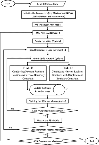
SelfSim algorithm is able to extract the non-linear stress–strain relations directly from the global response of structures such as forces and displacements [7] that should be measured from testing. Details on setting parameters for SelfSim can be referred to [29]. The SelfSim analysis runs two independent and parallel non-linear finite element analyses. One of them is a force-controlled analysis (FEM-FC) and the other one is a displacement-controlled analysis (FEM-DC). These two analyses are incrementally run until the last load (or time) step. Schematic procedures for the SelfSim are illustrated in Figure 1. In SelfSim, a complete load (or time) steps is called one ANN Pass.

Figure 1. Simplified flowchart of SelfSim framework.

2.1. Pre-training

Before starting the SelfSim training, the ANN model should be pre-trained with linear elastic behaviour. According to numerous SelfSim simulation tests, the number of pre-training epochs is preferably to be set at 1000. Since the neural network model is pre-trained with linear elastic behaviour with the number of epochs 1000 before auto-progressive training, initial prediction of stresses is quite accurate and practically there is no issue in convergence with the initial guess.

2.2. Procedures of SelfSim training

After pre-training, ANN Pass starts as seen in Figure 1. At each load or time step, a maximum of three auto-progressive cycles are carried out. Based on experiences with various numerical tests,[10] three is the suitable number for auto-progressive cycles that allow a gradual learning of the constitutive behaviour of materials. Standard Newton–Rahpson iteration is nested inside the auto-progressive cycles. During intermediate auto-progressive cycles, stresses and strains are collected from FEM-FC and FEM-DC, respectively, after solutions are converged in the current load or time step. The newly constructed input pattern to the ANN model is appended to the training database, and the ANN model is retrained with the updated training database. If the number of auto-progressive cycles does not reach the maximum value (i.e. three) or if the displacement error (i.e. difference between computed displacements and reference displacements) from the FEM-DC analysis is still larger than a user-defined tolerance, then the appended training data are removed from the accumulated training database, and the next auto-progressive cycle is continued. Otherwise, the auto-progressive cycle in the current load or time step is stopped, and the next load or time step continues keeping the new appended training data in the database. After the final auto-progressive cycle is completed or the displacement error is converged within the tolerance, stresses and strains are appended to the training database and SelfSim training continues to the next load step until completing one ANN Pass. If necessary, further ANN Passes can be conducted to increase the predictability of the extracted ANN material model. However, as mentioned previously, owing to the new internal variable used in the input pattern, one ANN Pass could be enough. In each auto-progressive cycle, the number of epochs is set to 100 for the SelfSim training. This helps to avoid premature training with stress and strain data from the early load or time steps.

A MATLAB code was developed to implement the SelfSim analysis. For the FE simulation, the code was linked to a general purpose commercial FE programme, ABAQUS. The ANN code was implemented in a user subroutine (UMAT) of the ABAQUS. The ANN model was also updated there after each increment. In the current framework, the post-processing was done by automatic utility routines and FORTRAN codes.

3. Genetic programming

Computational intelligence (CI) techniques are well-known predictive tools. CI includes ANNs and evolutionary algorithms (EAs) that use biology-inspired mechanisms to optimize a solution for desired results. In the past two decades, developments in the computer hardware and software have made it feasible for these techniques to grow. In addition, it has been proven that CI approaches are utilized as efficient predictive tools in real-world problems where conventional approaches fail or perform poorly. Using the principle of Darwinian natural selection, GP is an EA technique that creates computer programs to solve a problem. GP emerged in the late 1980s with the experiments on symbolic regression by Koza [30]. This traditional GP technique is also referred to as tree-based GP.[18] GP can be considered as an extension of GA. In GP, its evolving programmes (individuals) are parse trees rather than fixed or variable-length binary strings in GA.

In order to carry out GA-based optimizations, one or more objective function(s) should be pre-defined as objective(s). However, GP can generate prediction equations without any need to assume prior form of the relationship(s) or to pre-define function(s). A survey of the literature reveals the increasingly growing interests in GP from various fields of engineering community.

3.1. LGP

LGP is a recent variant of GP with a linear representation of programmes. In comparison with traditional GP, there are two main differences of LGP and traditional tree-based GP. The first one is about their structures. In LGP, expressions of a functional programming language are replaced by programmes of an imperative language (e.g. LISP is substituted by C/C++).[31] Figure 2 clearly shows the different programme structures in LGP and the tree-based GP. As it can be observed in Figure 2, a LGP is a data flow generated using several register contents. As can be seen from Figure 2(b), the data flow is more rigidly determined in the tree-based GP, by the tree structure of the programme. This allows linear solutions to express more complex calculations with less instructions and to be more compact in size in comparison with tree solutions.[31]

Figure 2. Comparison of the GP programme structures. (a) LGP (b) Tree-based GP [32].

Another basic difference between a linear programme and a tree programme is that LGP has ‘non-effective’ code segments which coexist with ‘effective’ code.[33] Non-effective codes of LGP programmes do not have any influence on the programme behaviour while effective codes have some influence on it. Non-effective codes are LGP advantages because they allow variations to remain neutral in terms of fitness change and also reduce the effect of variation on the effective code.[31] Due to the linear structure in LGP, detecting and eliminating non-effective parts is easier than other GPs and similar systems.[34] Thus, the linear genetic programme is more efficiently interpreted. LGP can remove the non-effective codes before a programme is executed during fitness evaluation. In this process, all effective instructions are copied to a temporary programme buffer and this accelerates the LGP execution speed.[35]

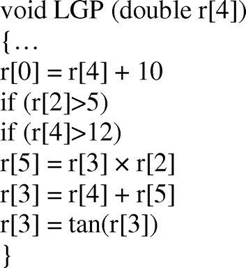
In the LGP system, a variable-length sequence of simple C instructions represents each individual programme. The function set or instruction set includes function calls, arithmetic operations and conditionals. The terminal set of the system can be constants or variables. The instructions are limited to operations that accept a minimum number of constants (or memory variables), called registers (r), and assign the result to a register (e.g. r₀: = r₁ + 1).[35] Part of a sample C code corresponding to the linear genetic programme is illustrated in Figure 3. From this figure, register parameters r[0] holds the final programme output.

Figure 3. An excerpt of a linear genetic programme.

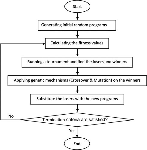
Automatic induction of machine code by genetic programming (AIMGP) is a special form of LGP. In AIMGP, the genetic programmes are stored as linear strings of native binary machine codes. Then the linear strings are directly executed by a processor during the fitness evaluation. The machine code-based LGP execution is much faster than the tree-based GP due to the absence of an interpreter and complex memory handling in AIMGP.[33] This LGP searches the constants and the computer program at the same time. Figure 4 shows a simplified flowchart of the LGP algorithm for a single run. More detail about the LGP can be found at [31].

Figure 4. Simplified flowchart of the LGP.

3.2. GP for constitutive behaviour modelling

There are a few efforts in the literature to apply EAs for constitutive behaviour modelling. Feng and Yang [36] used a hybrid evolutionary algorithm for recognizing the constitutive law for laminated composites. Javadi and Rezania [37] applied evolutionary polynomial regression to modelling of non-linear material constitutive laws. They used the evolutionary techniques for curve fitting on the experimental stress–strain curve.

To verify the applicability of GP to the non-linear stress–strain relationship, the LGP is applied into two different stress–strain curves. Two experimental databases containing stress–strain relationships were used here. The first one is the stress–strain relationship of soil obtained from the unconfined compression test data.[38] The second one is obtained from a structural basis study of the stress–strain relation of aorta presented in [39].

For the GP analyses, the available data-sets are randomly divided into three subsets including learning, validation and testing. The learning and validation data-sets are used to select the best evolved programmes and included in the training process. The testing data are used for performance measurements of the models. Out of the whole data, 85% data are used as the training data (70% as the learning data and 15% as the validation data). The remaining 15% data-sets are taken for testing the generalization capability of the models.

Different parameters involved in the LGP algorithm are presented in Table 1. Their selection has many effects on the model generalization capability. Several runs were conducted to tune the LGP parameters for sufficient robustness and generalization required to solve the problem. The parameters were selected according to some previously suggested values [40–43] and also after trial studies. Two levels are set for the population size, and crossover and mutation rates. Although most GP systems benefit from a very low mutation rate, LGP uses a much higher mutation rate.[43] From Table 1, large values are also considered for population size, because both a high mutation rate and a larger population size guarantee higher code diversity in the population.[31] The initial and maximum programme sizes are, respectively, set to optimal values of 80 and 128 bytes as trade-offs between complexity of the evolved solutions and running time. The number of demes is set as 20. This parameter is related to the manner in which the programmes population is divided. It should be noted that demes are semi-isolated subpopulations that evolution proceeds faster in them in comparison to a single population of equal size.[17] In this study, basic arithmetic operators and mathematical functions were utilized to get the optimum LGP models. There are 2³ = 8 different combinations of the parameters (i.e. population size, crossover and mutation rates). These combinations were tested and five replications for each combination were carried out. Therefore, the overall number of runs was 8  ×  5 = 40. A fairly large number of tournaments, which slightly the computational cost, were tested on each run to find models with minimum mean squared error (MSE). For each case, the programme is run until there is no significant improvement in the performance of the models or the runs were terminated automatically. For the LGP-based analysis, the Discipulus S/W [44] was used that works on the AIMGP platform. In LGP, four programmes (constitutive equations) were selected as two losers and two winners. Therefore, it works as a steady-state GP which is very fast converged algorithm.

Table 1. Parameter settings for the LGP algorithm.

Parameter	Settings
Function set	+, -, ×, /, √
Population size	500, 1000
Maximum number of tournaments	10,000
Maximum programme size	128
Initial programme size	80
Crossover rate (%)	50, 95
Homologous crossover (%)	95
Mutation rate (%)	50, 95
Block mutation rate (%)	30
Instruction mutation rate (%)	30
Data mutation rate (%)	40
Number of demes	20

In modelling of the constitutive law behaviour there are some physical constraints that should be satisfied. The most important physical constraint is that when there is no strain, the stress should be equal to zero, assuming no initial stresses. This causes numerical errors on FE analysis and its convergence may not happen. Therefore, the obtained model may not be useful for forward analysis. Hence, to remove this issue, the GP output is changed to:(3) $$\mathit{\sigma }=Linearpart+Nonlinearpart=E\mathit{\epsilon }+Nonlinearpart=E\mathit{\epsilon }\left(1+f_{GP}\left(\mathit{\epsilon }\right)\right)$$(3)

where E is the linear elastic Young’s modulus that can be easily obtained from experimental test results or pre-training of SelfSim.

The best GP correlation is chosen on the basis of a multi-objective strategy as follows:

(1)	The simplicity of the model, although this is not a predominant factor.
(2)	Providing the best fitness value on the learning set of data.
(3)	Providing the best fitness value on the validation set of data.

The first objective can be controlled by the user through the parameter settings (e.g. maximum programme depth). However, for more complex problem with more variables, it is required to use a multi-objective GP to work out a Pareto trade-off between the accuracy and complexity of the GP models.[45,46] For the other objectives, the following objective function (OBJ) was constructed as a measure of how well the model-predicted output agrees with the measured output. The selections of the best models were deduced by the minimization of the following function [47]:(4) $$\text{OBJ}=\left(\frac{N{o}_{Learning}-N{o}_{Validation}}{N{o}_{Training}}\right)\frac{RMS{E}_{Learning}+MA{E}_{Learning}}{R_{Learning}^2}+2\frac{N{o}_{Validation}}{N{o}_{Training}}\times \frac{RMS{E}_{Validation}+MA{E}_{Validation}}{R_{Validation}^2}$$(4)

where No. is the abbreviation of number of sets, R is the correlation coefficient, RMSE is the root MSE and MAPE is the mean absolute percent error.

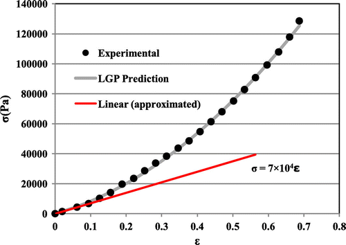
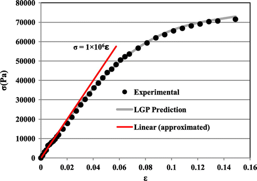
For the soil modelling case, the best LGP model (see the Appendix 1) is selected on the basis of the OBJ value. After interpreting the C code, the LGP-based formula is obtained which is presented in Equation (5(5) $$f_{LGP}\left(\mathit{\epsilon }\right)=\mathit{\epsilon }\left(2{\left(8\mathit{\epsilon }-1\right)}^2-3.5\right)$$(5) ). A comparison of the experimental stress–strain relationship versus predicted relationship values is shown in Figure 5. This figure also shows the approximated linear elastic modulus.(5) $$f_{LGP}\left(\mathit{\epsilon }\right)=\mathit{\epsilon }\left(2{\left(8\mathit{\epsilon }-1\right)}^2-3.5\right)$$(5)

Figure 5. Experimental vs. predicted stress–strain relationship for soils under unconfined compression.

For the second case, the LGP-based prediction equation is as follows:(6) $$f_{LGP}\left(\mathit{\epsilon }\right)=2\sqrt{\mathit{\epsilon }\left(1.\overline{4}\mathit{\epsilon }-0.0\overline{5}\right)}$$(6)

Figure 6 shows the experimental and predicted stress–strain values as well as approximated linear elastic modulus.

Figure 6. Experimental vs. predicted stress–strain relationship for aorta.

Results of these two examples clearly show that GP can predict the stress–strain relationship with high degrees of accuracy. In the next section, we have combined SelfSim with GP for constitutive law modelling.

4. Coupled SelfSim and genetic programming

The ANN-based material constitutive model is powerful and it can be applied to any unknown material.[48–51] However, ANN-based material constitutive models seem to be more suitable for natural granular materials, such as soils and rocks, and it is difficult to derive generalized material constitutive models in explicit mathematical forms. The complexities of the ANN-based models in implementations to general purpose finite element codes, such as ABAQUS and ANSYS, also motivates the proposed idea.[16]

Although ANNs have been successful in forecasting; in general, they are not able to produce practical prediction equations. Furthermore, they require the structure of the network (e.g. transfer functions, number of hidden layers, etc.) to be identified a priori. The ANN method is mostly appropriate to be used as a part of a computer program and it also restricts their usefulness.

Generally, GP training takes far more than ANN training. Therefore, it is not practical to use GP in SelfSim framework as it is needed to develop a model in each iteration. As mentioned in the last section, using the classical framework of SelfSim with ANN may not be able to satisfy the physical constraint, that is, zero stress at zero strain. This may be responsible for numerical error in FE analysis and may affect the convergence.

In this section, we have combined advantages of the SelfSim and GP framework proposed in the last section in order to overcome these issues and maximize the usefulness of the SelfSim and GP algorithms. SelfSim is used for extracting realistic stress–strain fields that could be in complex stress states over the loading history. GP is used for formulating the explicit mathematical form of the non-linear constitutive models.

The combined algorithm is on the basis of three main run steps:

(1)	Run SelfSim analysis and derive an ANN-based model for the material behaviour.
(2)	Run forward analysis under displacement controls to extract the stress–strain database.
(3)	Run GP on the database and formulate the material model in an explicit mathematical form.

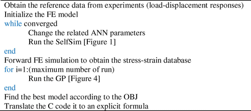
It should be noted that, as the constitutive law is the same for all elements (assuming that structures are made of the same materials) and also for uniform distribution of data for GP modelling, only stress–strain of the highest stressed element was used for GP training. This sequentially coupled algorithm can formulate the constitutive law of each material only using the load–deflection response. The simplified pseudo-code of this hybrid algorithm is show in Figure 7.

Figure 7. Simplified pseudo-code of SelfSim–GP algorithm.

4.1. Case study: space truss

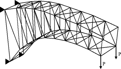
To demonstrate the feasibility of the SelfSim-GP algorithm, a space truss structure containing 40 nodes and 112 elements was used (see Figure 8). In order to create the hypothetical reference material model, Ramberg–Osgood-type plasticity model was used here.

Figure 8. Space truss structure used in case study.

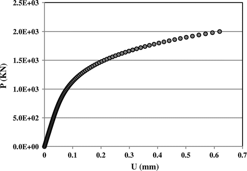
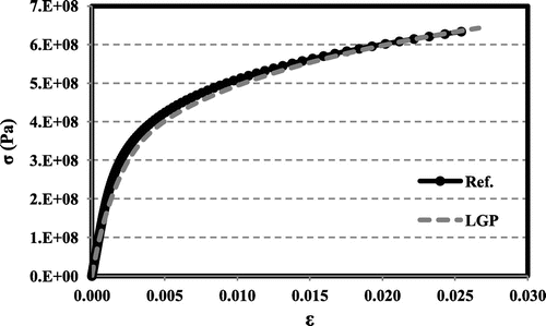
The global force–displacement response of the structure at the point of applied forces is shown in Figure 9. These data were gathered after 100 load steps.

Figure 9. Global force–displacement response of the truss structure.

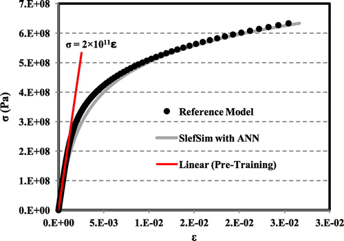
Using the global responses, the SelfSim framework was run. As it is mentioned, the parallel non-linear FE analyses by ABAQUS were controlled by MATLAB. The ANN code is also developed in UMAT. The inputs of the ANN model were ε_n, ε_n−1, σ_n−1, ξ_ε,n and the output was σ_n. The ANN model has two hidden layers and each hidden layer has 25 neurons. The ANN results after pre-training and full auto-progressive training cycles, and the stress–strain relationship from the most highly stressed element of the reference model are shown in Figure 10.

Figure 10. Stress–strain behaviour modelling using ANN.

The GP model was obtained by using the database generated from a forward FE simulation following the SelfSim simulation. The best programme (see the Appendix 1) was also selected based on the minimum objective function value in Equation (4(4) $$\text{OBJ}=\left(\frac{N{o}_{Learning}-N{o}_{Validation}}{N{o}_{Training}}\right)\frac{RMS{E}_{Learning}+MA{E}_{Learning}}{R_{Learning}^2}+2\frac{N{o}_{Validation}}{N{o}_{Training}}\times \frac{RMS{E}_{Validation}+MA{E}_{Validation}}{R_{Validation}^2}$$(4) ). The GP-based formula after translating the programme is:(7) $$f_{GP}\left(\mathit{\epsilon }\right)=\frac{\mathit{\epsilon }+{\left(\mathit{\epsilon }+\mathit{\alpha }\right)}^2}{4\mathit{\epsilon }+12\sqrt[4]{\mathit{\epsilon }}-6\sqrt[3]{\mathit{\epsilon }}-\mathit{\alpha }-{\left(\mathit{\epsilon }+\mathit{\alpha }\right)}^2}$$(7) (8) $$\mathit{\alpha }={\left(6\mathit{\epsilon }+12\sqrt[4]{\mathit{\epsilon }}-4\sqrt[3]{\mathit{\epsilon }}\right)}^2$$(8)

Finally the GP-based constitutive model was obtained after plugging Equation (7(7) $$f_{GP}\left(\mathit{\epsilon }\right)=\frac{\mathit{\epsilon }+{\left(\mathit{\epsilon }+\mathit{\alpha }\right)}^2}{4\mathit{\epsilon }+12\sqrt[4]{\mathit{\epsilon }}-6\sqrt[3]{\mathit{\epsilon }}-\mathit{\alpha }-{\left(\mathit{\epsilon }+\mathit{\alpha }\right)}^2}$$(7) ) in Equation (3(3) $$\mathit{\sigma }=Linearpart+Nonlinearpart=E\mathit{\epsilon }+Nonlinearpart=E\mathit{\epsilon }\left(1+f_{GP}\left(\mathit{\epsilon }\right)\right)$$(3) ).

4.2. Forward FE simulation using GP-based constitutive model

After obtaining the LGP-based constitutive model, the model has been implemented in UMAT subroutine of the ABAQUS to check its workability and convergence. In UMAT, current strains are passed from the ABAQUS main module and stresses should be updated and Jacobian stiffness matrix should be calculated. The stress can simply be updated using the explicit GP-based constitutive model. As the Jacobian tangent material moduli are defined as(9) $$J=\frac{\mathit{\partial }\mathit{\sigma }}{\mathit{\partial }\mathit{\epsilon }},$$(9)

the Jacobin can be calculated by a direct differentiation of Equation (3(3) $$\mathit{\sigma }=Linearpart+Nonlinearpart=E\mathit{\epsilon }+Nonlinearpart=E\mathit{\epsilon }\left(1+f_{GP}\left(\mathit{\epsilon }\right)\right)$$(3) ). A comparison of reference stress–strain relationship for the highest stressed element and LGP model is presented in Figure 11. As it can be seen, the prediction results are highly correlated to the reference model (R = 0.99999991). The comparison of the stress–strain distribution of the whole structure after FE analysis using the actual material model and the constitutive model derived by SelfSim–GP methodology is illustrated in Figure 12.

Figure 11. A comparison of reference model, ANN-based model and GP model.

Figure 12. Stress–strain distribution of the whole structure. (a) Reference material model, (b) GP-based material model derived by SelfSim–GP methodology.

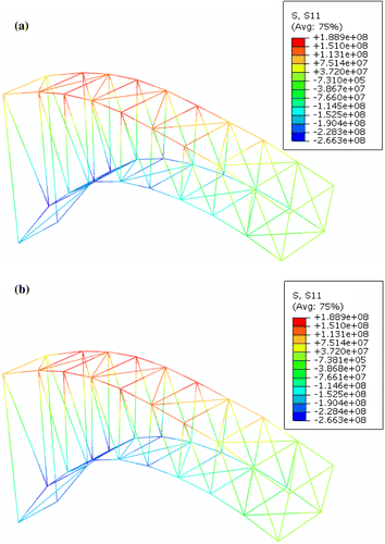
As it can be seen from these figures, the results of FE simulation using the SelfSim–LGP-based constitutive model is very close to the reference model. This clearly shows the possibility of the LGP constitutive model implementation.

5. Summary and conclusion

The SelfSim and GP have been systematically coupled for developing non-linear material constitutive laws from global load–displacement histories on the structures. In this paper, a powerful numerical inverse analysis framework SelfSim was used for learning and extracting material constitutive models in ANN forms. The ANN-based material constitutive models can potentially learn complex stress–strain behaviour of real-life structures for its highly adaptable and learning capabilities. The complex stress–strain database could be extracted from ANN-based forward finite element analyses. Subsequently, a recent and robust variant of GP namely LGP was employed for developing non-linear material constitutive models.

At first, the LGP was tested for constitutive modelling using two experimental stress–strain databases, i.e. soils under unconfined compression and aorta. After verification of the LGP for constitutive behaviour modelling, the coupled SelfSim-GP algorithm was tested using a hypothetical truss structure. For testing the usefulness of the model, the forward FE simulation was also done using the GP-based material model. The proposed material constitutive model is implemented in UMAT subroutine of ABAQUS software.

The proposed methodology combined the advantages of the SelfSim and GP frameworks and potentially increased the usefulness of the constitutive model. Using the GP, the model changed from a black box model to an explicit formula which can be used for Jacobian stiffness matrix calculation. The GP-based model is so accurate with correlation coefficient close to one which is also visualized. Validation of the proposed model by a forward FE simulation shows that the structural responses using the GP-based constitutive model are almost same as those of reference material model. These results clearly show the algorithm performance and convergence as well as its workability in practice.

Additional information

Funding

Funding. This research is supported by the New Faculty Startup Fund from the University of Akron. The authors are grateful for this support.

Appendix 1

^{Table A1}

Table A1. The optimum LGP programmes of the case studies which can be run in the Discipulus interactive evaluator mode or can be compiled in C++ environment. (Note: v[0], represents ε).

Case I (soil compression model)	Case II (structural aortic model)	Case III (ANN-based material model)
float Discipulus C Function (float v[])	float Discipulus C Function (float v[])	float Discipulus C Function (float v[])
{	{	{
double f[8];	double f[8];	double f[8];
double tmp = 0;	double tmp = 0;	double tmp = 0;
f[1]=f[2]=f[3]=f[4]=f[5]= f[6]=f[7]=f[8]= 0;	f[1]=f[2]=f[3]=f[4]=f[5]=f[6]=f[7]=f[8]= 0;	f[1]=f[2]=f[3]=f[4]=f[5]=f[6]=f[7]=f[8]= 0;
f[0]=v[0];	f[0]=v[0];	f[0]=v[0];
l0: f[0]/=0.25;	l0: f[0]+=f[0];	l0: f[0]*=8;
l1: f[0]−=0.5;	l1: f[0]+=f[0];	l1: f[0]=sqrt(f[0]);
l2: f[0]*=f[0];	f[1]+=f[0];	f[1]−=f[0];
l3: f[0]+=f[0];	l2: f[0]−=0.5;	l2: f[0]−=0.25;
f[0]+=f[0];	l3: l4: f[0]/=9;	l3: f[0]*=f[0];
l4: f[0]+=f[0];	l5: f[0]+=v[0];	f[1]+=f[0];
l5: f[0]+=0.5;	l6: f[0]*=f[0];	l4: f[1]+=f[0];
l6: f[0]−=4;	f[0]=sqrt(f[0]);	f[0]+=f[1];
l7: f[0]*=v[0];	l7: f[0]*=f[1];	l5: f[0]=fabs(f[0]);
l8:	f[0]=sqrt(f[0]);	f[0]−=f[1];
l9:	l8:	l6: f[1]−=f[0];
return f[0];	l9:	f[0]*=f[0];
}	return f[0];	l7: f[0]*=f[0];
	}	f[0]+=f[1];
		l8:
		l9:
		return f[0];
		}

References

- Gandomi AH, Alavi AH, Sahab MG, Arjmandi P. Formulation of elastic modulus of concrete using linear genetic programming. J. Mech. Sci. Technol. 2010;24:1273–1278.
- Xia Z, Ellyin F, Meijer G. Mechanical behavior of Al2O3-particle-reinforced 6061 aluminum alloy under uniaxial and multiaxial cyclic loading. Compos. Sci. Technol. 1997;57:237–248.
- Choi Y, Han CS, Lee JK, Wagoner RH. modeling multi-axial deformation of planar anisotropic elasto-plastic materials, part 1: theory. Int. J. Plast. 2006;22:1745–1764.
- Alavi AH, Gandomi AH. Prediction of principal ground-motion parameters using a hybrid method coupling artificial neural networks and simulated annealing. Comput. Struct. 2011;89:2176–2194.
- Pernot S, Lamarque CH. Application of neural networks to the modelling of some constitutive laws. Neural Networks. 1999;12:371–392.
- Han YF, Zeng WD, Zhao YQ, Zhang XM, Sun Y, Ma XO. Modeling of constitutive relationship of Ti-25 V-15Cr-0.2Si alloy during hot deformation process by fuzzy-neural network. Mate. Des. 2010;31:4380–4385.
- Ghaboussi J, Pecknold DA, Zhang MF, Haj-Ali RM. Autoprogressive training of neural network constitutive models. Int. J. Numer. Methods Eng. 1998;42:105–126.
- Pettersson F, Chakraborti N, Saxen H. A genetic algorithms based multi-objective neural net applied to noisy blast furnace data. Appl. Soft Comput. 2007;7:387–397.
- Mondal DN, Sarangi K, Pettersson F, Sen PK, Saxen H, Chakraborti N. Cu-Zn separation by supported liquid membrane analyzed through multi-objective genetic algorithms. Hydrometallurgy. 2011;107:112–123.
- Yun G, Saleeb A, Shang S, Binienda W, and Menzemer C. Improved selfsim for inverse extraction of nonuniform, nonlinear, and inelastic material behavior under cyclic loadings. J. Aerosp. Eng. 2012;25:256–272.
- Yun GJ, Ghaboussi J, Elnashai AS. Self-learning simulation method for inverse non-linear modeling of cyclic behavior of connections. Comput. Methods Appl. Mech. Eng. 2008;197:2836–2857.
- Sidarta D, Ghaboussi J. Constitutive modeling of geomaterials from non-uniform material tests. Comput. Geotech. 1998;22:53–71.
- Shin HS, Pande GN. On self-learning finite element codes based on monitored response of structures. Comput. Geotech. 2000;27:161–178.
- Ghaboussi J, Sidarta D. A new nested adaptive neural network for modeling of constitutive behavior of materials. Int. J. Comput. Geotech. 1998;22:29–51.
- Tsai CC. Seismic site response and interpretation of dynamic soil behavior from down hole array measurements [Ph.D. thesis]. Urbana: University of Illinois Urbana-Champaign; 2007.
- Banzhaf W, Nordin P, Keller R, Francone F. Genetic programming – an introduction: on the automatic evolution of computer programs and its application. San Francisco (CA): Morgan Kaufmann; 1998.
- Koza JR. Genetic programming: on the programming of computers by means of natural selection. Cambridge (MA): MIT Press; 1992.
- Gandomi AH, Alavi AH. Multi-stage genetic programming: a new strategy to nonlinear system modeling. Inf. Sci. 2011;181:5227–5239.
- Gandomi AH, Yun GJ, Alavi AH. An evolutionary approach for modeling of shear strength of RC deep beams. Mater. Struct. 2013;46:2109–2119.
- Gandomi AH, Alavi AH, Yun GJ. Nonlinear modeling of shear strength of SFRC beams using linear genetic programming. Struct. Eng. Mech. 2011;38:1–25.
- Azamathulla HM, Guven A, Demir YK. Linear genetic programming to scour below submerged pipeline. Ocean Eng. 2011;38:995–1000.
- Oltean M, Grossan C. A comparison of several linear genetic programming techniques. Complex Syst. 2003;14:1–29.
- Gandomi AH, Alavi AH. Applications of Computational Intelligence in Behavior Simulation of Concrete Materials. In: Yang XS, Koziel S, editors. Computational optimization & applications. Berlin: Springer-Verlag; 2011. p. 221–243.
- Jung S, Ghaboussi J. Characterizing rate-dependent material behaviors in self-learning simulation. Comput. Methods Appl. Mech. Eng. 2006;196:608–618.
- Jung S, Ghaboussi J, Marulanda C. Field calibration of time-dependent behavior in segmental bridges using self-learning simulation. Eng. Struct. 2007;29:2692–2700.
- Yun GJ, Ghaboussi J, Elnashai AS. Development of neural network based hysteretic models for steel beam-column connections through self-learning simulation. J. Earthquake Eng. 2007;11:453–467.
- Yun GJ, Ghaboussi J, Elnashai AS. A new neural network-based model for hysteretic behavior of materials. Int. J. Numer. Methods Eng. 2008;73:447–469.
- Yun GJ, Saleeb AF, Shang S, Binienda W, Menzemer C. Improved SelfSim for inverse extraction of non-uniform, nonlinear and inelastic constitutive behavior under cyclic loadings. J. Aerosp. Eng. 2012;25:256–272.
- Koza J. Hierarchical genetic algorithms operating on populations of computer programs. In: Sridharan N, Kaufmann M, editors. In Proceedings of the 11th Internatinal Joint Conference on Artificial Intelligence. San Mateo (CA); 1989. p. 768–774.
- Brameier M, Banzhaf W. Linear genetic programming (genetic and evolutionary computation). New York (NY): Springer; 2007.
- Gandomi AH, Alavi AH, Hosseini SS. A discussion on ‘Genetic programming for retrieving missing information in wave records along the west coast of India’. Appl. Ocean Res. 2008;30:338–339. 2007;29:99–111.
- Brameier M, Banzhaf W. A comparison of linear genetic programming and neural networks in medical data mining. IEEE Trans. Evol. Comput. 2001;5:17–26.
- Francone FD, Deschaine LM. Extending the boundaries of design optimization by integrating fast optimization techniques with machine-code-based, linear genetic programming. Inf. Sci. 2004;161:99–120.
- Alavi AH, Gandomi AH, Mollahasani A, Bolouri Bazaz J. Linear and tree-based genetic programming for solving geotechnical engineering problems. In: Yang XS, Gandomi AH, Alavi AH, Talatahari S, editors. Metaheuristics in water, geotechnical and transportation engineering. London: Elsevier; 2013. p. 289–310.
- Feng X, Yang C. Coupling recognition of the structure and parameters of non-linear constitutive material models using hybrid evolutionary algorithms. Int. J. Numer. Methods Eng. 2004;59:1227–1250.
- Javadi AA, Rezania M. Intelligent finite element method: an evolutionary approach to constitutive modeling. Adv. Eng. Inf. 2009;23:442–451.
- Reddy K. Experiment 12: unconfined compression (UC) test. Chicago (IL): University of Illinois at Chicago; 2002.
- Sokolis DP, Kefaloyannis EM, Kouloukoussa M, Marinos E, Boudoulas H, Karayannacos PE. A structural basis for the aortic stress–strain relation in uniaxial tension. J. Biomech. 2006;39:1651–1662.
- Gandomi AH, Alavi AH, Sahab MG. New formulation for compressive strength of CFRP confined concrete cylinders using linear genetic programming. Mater. Struct. 2010;43:963–983.
- Alavi AH, Gandomi AH. A robust data mining approach for formulation of geotechnical engineering systems. Eng. Comput. 2011;28:242–274.
- Alavi AH, Gandomi AH. Energy-based numerical models for assessment of soil liquefaction. Geosci. Front. 2012;3:541–555.
- Francone FD. Discipulus ProTM software owner’s manual. Littleton (CO): Register Machine Learning Technologies Inc.; 2001.
- Conrads M, Dolezal O, Francone FD, Nordin P. Discipulus–fast genetic programming based on AIM learning technology. Littleton: Register Machine Learning Technologies Inc.; 2004.
- Giri BK, Hakanen J, Miettinen K, Chakraborti N. Genetic programming through bi-objective genetic algorithms with a study of a simulated moving bed process involving multiple objectives. Appl. Soft Comput. 2013;13:2613–2623.
- Giri BK, Pettersson F, Saxen H, Chakraborti N. Genetic Programming Evolved through Bi-Objective Genetic Algorithms Applied to a Blast Furnace. Mater. Manuf. Processes. 2013;28:776–782.
- Gandomi AH, Alavi AH, Mousavi M, Tabatabaei SM. A hybrid computational approach to derive new ground-motion prediction equations. Eng. Appl. Artif. Intell. 2011;24:717–732.
- Ghaboussi J, Garrett J, Wu X. Knowledge‐based modeling of material behavior with neural networks. J. Eng. Mech. ASCE. 1991;117:132–153.
- Haj-Ali R, Kim HK. Nonlinear constitutive models for FRP composites using artificial neural networks. Mech. Mater. 2007;39:1035–1042.
- Shen Y, Chandrashekhara K, Breig WF, Oliver LR. Neural network based constitutive model for rubber material. Rubber Chem. Technol. 2004;77:257–277.
- Sun Y, Zeng WD, Zhao YQ, Qi YL, Ma X, Han YF. Development of constitutive relationship model of Ti600 alloy using artificial neural network. Comput. Mater. Sci. 2010;48:686–691.