Riemannian methods for optimization in a shape space of triangular meshes

Abstract

In this paper, the applicability of two optimization algorithms in the context of Riemannian manifolds is investigated. More precisely, the steepest descent method and the nonlinear conjugate gradient method are used to solve the Shape-From-Shading problem in a shape space of triangular meshes. For this reason, appropriate Riemannian metrics are introduced in this shape space. Instead of taking steps along straight lines, propagation along geodesics with respect to the Riemannian metric is employed. This requires to formulate the geodesic equation and the equation of parallel translation in the shape space of triangular meshes. In general, the proposed geodesic optimization algorithms outperform the standard steepest descent method concerning various quality measures and the visual impression of the reconstructed surface. In addition, it is shown that an appropriately chosen Riemannian metric can guide the optimization process towards a desired class of surfaces.

Keywords:

• shape optimization
• shape space
• Riemannian manifold
• geodesic
• parallel transport
• shape-from-shading

AMS Subject Classifications:

• Primary: 49Q10
• Secondary: 53B21
• 65D17

1 Introduction and prerequisites

The solution of optimization on differentiable manifolds is – on the one hand – a very well investigated field, especially if dealing with embedded implicit manifolds. In this case, the manifold $M^{n-k}$ is the geometric locus of the solution to the equation $\mathbf{h}(\mathbf{x})=\mathbf{0}$ with $\mathbf{h}\in {\mathcal{C}}^1({\mathbb{R}}^n,{\mathbb{R}}^k)$ and the whole extremely well-developed machinery of constrained optimization applies. The iterative optimization problem is set up in the embedding space and produces either feasible points which lie on the manifold in every step or infeasible points for which only the limit of the sequence of approximate solutions is an element of $M^{n-k}$. If the manifold is either not embedded or already given in (local) coordinates, the situation seems even less complicated because the optimization algorithm can be set up in parameter space and the available techniques of unconstrained optimizations apply, with the possible complication that the parametrization might have to be changed if the sequence of approximate solutions leaves a coordinate patch. It is, however, obvious that one and the same algorithm will produce very different iterates if applied within different coordinate systems. Especially, the measurement of step lengths, distances between subsequent iterates, angles which will be used in projection formulas etc. will be dependent on the coordinate system and might not reflect the actual geometry of the manifold.

It has been suggested by several authors (see e.g. [1] or the monograph [2]) to use an appropriate Riemannian structure on the manifold for the metric aspects occurring in optimization algorithms. Moreover, geodesics (see [3] for an introduction) on the manifold can be viewed as a natural generalization of straight lines in vector space. Consequently, geodesics can be used to define lines along which the cost functional decreases and which serve as one-dimensional search regions. It has been shown that gradient-type, Newton-type and Quasi-Newton or CG-type algorithms can be formulated and analysed in the Riemannian context. The use of differential geometric methods for the solution of optimization problems over feasible sets of geometric variables $\mathrm{\Omega }\subset {\mathbb{R}}^n$ is rather a recent development. The terminology ‘shape space’ is used in this context as an umbrella term for sets of geometric variables endowed with an appropriate topological, metric or differential structure. Mumford and Michor [4] introduced a general class of metrics on equivalence classes of parametrized curves obtaining geometric metrical structures which are independent of the chosen parametrization. Even though the paper is not explicitly aimed towards optimization, it is manifest to use the construction of geodesics and parallel transport (see e.g. [3]) in shape space for the solution of problems in computer vision such as shape interpolation or shape identification. Pottman and co-workers constructed and implemented metrics on spaces of discretized surfaces in ${\mathbb{R}}^3$ also for the solution of problems occurring in computer vision. (See [5] for an overview.) Very recently, Schulz [6] presented a general framework for the construction and analysis of algorithms for the solution of shape optimization problems using a Riemannian structure on the underlying shape space. In [7] some classes of optimization algorithms on Riemannian manifolds using the concepts of geodesic propagation and parallel transport are analysed and applied in a shape space framework.

In this article, we discuss the steepest descent and the nonlinear conjugate gradient method formulated in the shape space of triangulated surfaces in ${\mathbb{R}}^3$ with $N$ nodes. See e.g. [8] for an introduction to the steepest descent and the nonlinear conjugate gradient method in vector spaces. The standard inner product in ${\mathbb{R}}^{3N}$ might not describe the underlying geometry of the shape space in an appropriate way. Consequently, the deformation of a surface corresponding to a straight line in the shape space is probably not a ‘natural’ evolution of the surface in ${\mathbb{R}}^3$. We, thus, endow this space with Riemannian metrics which give rise to geodesics different from straight lines. In principle, we construct the metrics in such a way that the resulting geodesics correspond to deformations which join different surfaces in the desired fashion. Our shape space versions of the steepest descent and the nonlinear conjugate gradient algorithm are essentially the same as their standard formulations up to the fact that steps along straight lines are replaced by steps along geodesics. This approach allows one to guide the optimization process in shape space within a certain class of surfaces.

The structure of the paper is the following. In the remainder of this introductory section, we provide standard concepts and results from differential geometry explaining geodesic and parallel movement in Riemannian manifolds. Section 2 is devoted to the introduction of a space of triangulated surfaces in ${\mathbb{R}}^3$ together with an appropriate tangent bundle. In Section 3, a class of metrics on the shape space is defined which measures the deviation from isometric distortion. The geodesic equation and the equation of parallel transport with respect to this class are derived. As a reference, the Euclidian metric in the parameter space is also investigated. The next Section 4 introduces the shape-from-shading problem and its formulation as a shape optimization problem. In Section 5, a steepest descent algorithm and a nonlinear conjugate gradient method are formulated in the described Riemannian framework. Several numerical experiments documented in Section 6 conclude the paper.

For the remainder of the paper, we make the following conventions. Every manifold is assumed to be a differentiable manifold; and every curve in a manifold is assumed to be of class $C^{\infty }$. In addition, we shall often use the notation$${\mathit{\partial }}_i:=\frac{\mathit{\partial }}{\mathit{\partial }{u}^i}$$for the basis vectors of the tangent space $T_p{M}^n$ to a manifold $M^n$ at a point $p\in M^n$. The set of all tangent vector fields on $M^n$ is denoted by $\mathcal{V}(M^n)$. If $M^n$ is a manifold with a (Pseudo-)Riemannian metric $⟨·,·⟩$, we denote the (pseudo-)metric tensor and its inverse by$$g_{ij}:=〈{\mathit{\partial }}_i,,,{\mathit{\partial }}_j〉\text{and}{g}^{ij}:={(G^{-1})}_{ij}\text{where}G:={(g_{ij})}_{ij}.$$Furthermore, we use the Einstein summation convention: Any index which occurs twice in a product is to be summed from $1$ up to the space dimension.

Definition 1

Let $M^n$ be a manifold. Then, a map $D:\mathcal{V}(M^n)\times \mathcal{V}(M^n)\to \mathcal{V}(M^n)$ is called a connection on $M^n$, if the following properties are satisfied for all $v,w,X,Y\in \mathcal{V}(M^n)$, $a,b\in \mathbb{R}$ and $f\in C^{\infty }(M^n)$:$$\begin{array}{cc}\hfill D_X(av+bw)& =a{D}_{X}v+b{D}_{X}w,\hfill \\ \hfill D_{aX+bY}v& =a{D}_{X}v+b{D}_{Y}v,\hfill \\ \hfill D_X(fv)& =X(f)v+f{D}_{X}v.\hfill \end{array}$$Moreover, we call a connection $D$torsion free if for all $X,Y\in \mathcal{V}(M^n)$,$$[X,Y]=D_{X}Y-D_{Y}X,$$where $[X,Y]$ denotes the Lie bracket. If $M^n$ is a Riemannian manifold with metric $⟨·,·⟩$, we call a connection $D$metric, if for all $Z\in \mathcal{V}(M^n)$,$$X⟨Y,Z⟩=⟨D_{X}Y,Z⟩+⟨Y,D_{X}Z⟩.$$

Definition 2

Let $M^n$ be a manifold with local coordinates $(u^1,\dots ,u^n)$ and $D$ be a connection on $M^n$. Then, the symbols ${\mathrm{\Gamma }}_{jk}^i$ defined via$$D_{{\mathit{\partial }}_j}{\mathit{\partial }}_k={\mathit{\partial }}_i{\mathrm{\Gamma }}_{jk}^i$$are called the coefficients of the connection $D$.

We have the following uniqueness result.[9]

Theorem 3

Let $M^n$ be a Riemannian manifold with metric $⟨·,·⟩$. Then, there exists a unique torsion free and metric connection $\mathrm{\nabla }:\mathcal{V}(M^n)\times \mathcal{V}(M^n)\to \mathcal{V}(M^n)$. This connection is given by$$⟨{\mathrm{\nabla }}_{X}Y,Z⟩=\frac{1}{2}(X⟨Y,Z⟩+Y⟨Z,X⟩-Z⟨X,Y⟩-⟨X,[Y,Z]⟩+⟨Y,[Z,X]⟩+⟨Z,[X,Y]⟩)$$and with local coordinates $(u^1,\dots ,u^n)$,$${\mathrm{\Gamma }}_{jk}^i=\frac{1}{2}{g}^{li}\left(\frac{\mathit{\partial }{g}_{lj}}{\mathit{\partial }{u}^k},+,\frac{\mathit{\partial }{g}_{kl}}{\mathit{\partial }{u}^j},-,\frac{\mathit{\partial }{g}_{jk}}{\mathit{\partial }{u}^l}\right).$$

In the situation of Theorem 3, the connection $\mathrm{\nabla }$ is called the Levi-Civita connection and its coefficients ${\mathrm{\Gamma }}_{jk}^i$ are called the Christoffel symbols.

Definition 4

Let $M^n$ be a Riemannian manifold, $x$ a curve in $M^n$, $Y\in \mathcal{V}(M^n)$ and $T\in \mathcal{V}(M^n)$ such that $T=dx/dt$ along $x$.

• $x$ is called a geodesic, if(1) $$\begin{array}{c}\hfill {\mathrm{\nabla }}_{T}T=0.\end{array}$$(1)

• $Y$ is said to be parallel displaced along $x$, if(2) $$\begin{array}{c}\hfill {\mathrm{\nabla }}_{T}Y=0.\end{array}$$(2)

Using the formula for the Christoffel symbols, we obtain the geodesic equation (3(3) $$\begin{array}{c}\hfill \frac{d^2{u}^i}{d{t}^2}+{\mathrm{\Gamma }}_{jk}^i\frac{d{u}^j}{dt}\frac{d{u}^k}{dt}=0\text{for all}i\in \{1,\dots ,n\}.\end{array}$$(3) ) and the equation of parallel translation (4(4) $$\begin{array}{c}\hfill \frac{d{Y}^i}{dt}+{\mathrm{\Gamma }}_{jk}^i\frac{d{u}^j}{dt}{Y}^k=0\text{for all}i\in \{1,\dots ,n\}.\end{array}$$(4) ) by expressing (1(1) $$\begin{array}{c}\hfill {\mathrm{\nabla }}_{T}T=0.\end{array}$$(1) ), respectively, (2(2) $$\begin{array}{c}\hfill {\mathrm{\nabla }}_{T}Y=0.\end{array}$$(2) ) in local coordinates.

Proposition 5

Let $M^n$ be a Riemannian manifold with local coordinates $(u^1,\dots ,u^n)$, $x=x(u(t))$ a curve in $M^n$, $Y\in \mathcal{V}(M^n)$ and $T\in \mathcal{V}(M^n)$ such that $T=dx/dt$ along $x$.

• $x$ is a geodesic,if and only if(3) $$\begin{array}{c}\hfill \frac{d^2{u}^i}{d{t}^2}+{\mathrm{\Gamma }}_{jk}^i\frac{d{u}^j}{dt}\frac{d{u}^k}{dt}=0\text{for all}i\in \{1,\dots ,n\}.\end{array}$$(3)

• $Y$ is parallel displaced along $x$, if and only if(4) $$\begin{array}{c}\hfill \frac{d{Y}^i}{dt}+{\mathrm{\Gamma }}_{jk}^i\frac{d{u}^j}{dt}{Y}^k=0\text{for all}i\in \{1,\dots ,n\}.\end{array}$$(4)

2 Optimization in the shape space of triangular meshes

In the sequel, we shall always consider the shape space $\mathcal{S}$ of triangulated meshes embedded in ${\mathbb{R}}^3$ with a fixed connectivity graph and a given number of nodes $N$. For a shape $M\in \mathcal{S}$ we will use $P\subset {\mathbb{R}}^3$ to denote the set of all nodes of $M$. For sure, $M$ and $P$ refer to the same object, the triangular mesh, but from different perspectives; on the one hand, $M$ describes the mesh as an element in an abstract shape space, whereas $P$ characterizes the mesh as a finite subset of ${\mathbb{R}}^3$. We also use the notation $\mathcal{N}(p)$ for the set containing $p$ and all nodes of $M$ which share a common edge with $p$ and call $\mathcal{N}(p)$ the set of all neighbours of $p$. Likewise, $\mathcal{T}(p)$ denotes the set of all triangles of $M$ which have $p$ as a vertex. Moreover, we define $C\subset P^2$ as the set of all $(p,q)\in P^2$ which are neighbours.

Since there is a one-to-one correspondence between meshes $M\in \mathcal{S}$ and vectors in ${\mathbb{R}}^{3N}$, we may identify the shape space $\mathcal{S}$ with ${\mathbb{R}}^{3N}$. However, to reconstruct the shape $M$ from a vector of $3N$ coordinates, knowledge of the local connectivity relation $C$ is necessary. Without this, the vector $x\in {\mathbb{R}}^{3N}$ represents only an unconnected point cloud. Using ${\mathbb{R}}^{3N}$ with its generic inner product as parameter space consequently means that the local geometry of the shape is not taken into account. In contrast – depending on the specific problem – we shall propose to use special Riemannian metrics to endow the shape space $\mathcal{S}$ with an appropriate geometry. Strictly speaking, these metrics have to be defined on each tangent space $T_M\mathcal{S}$ for $M\in \mathcal{S}$; this will be done below.

In the context of optimization, we are interested to define a consistent framework for the update of the shape variable (i.e. a deformation of the shape). We will restrict the admissible deformations of a triangular mesh to those which are normal to the surface. Specifically, every node $p\in P$ may only be moved along the local surface normal vector $n_p\in {\mathbb{R}}^3$. Consequently, our deformation fields are given by(5) $$\begin{array}{c}\hfill {(X_p)}_{p\in P}={({\mathit{\kappa }}_p{n}_p)}_{p\in P}\in T_M\mathcal{S}\end{array}$$(5) with ${\mathit{\kappa }}_p\in \mathbb{R}$. Hence, we do not consider all possible tangent vectors in the $3N$-dimensional tangent space $T_M\mathcal{S}$ but only vectors of the form (5(5) $$\begin{array}{c}\hfill {(X_p)}_{p\in P}={({\mathit{\kappa }}_p{n}_p)}_{p\in P}\in T_M\mathcal{S}\end{array}$$(5) ), which constitute an $N$-dimensional subspace of $T_M\mathcal{S}$. Mathematically speaking, a deformation of a mesh $M\in \mathcal{S}$ is a curve in $\mathcal{S}$ passing through $M$. Thus, we only consider curves in $\mathcal{S}$ whose tangent vectors are given by (5(5) $$\begin{array}{c}\hfill {(X_p)}_{p\in P}={({\mathit{\kappa }}_p{n}_p)}_{p\in P}\in T_M\mathcal{S}\end{array}$$(5) ). Therefore, all the admissible deformations of a surface $M\in \mathcal{S}$ are uniquely determined by the vector field $\overrightarrow{\mathit{\kappa }}:={({\mathit{\kappa }}_p)}_{p\in P}\in {\mathbb{R}}^N$ on $\mathcal{S}$. Now, we have to define properly the normal vector $n_p\in {\mathbb{R}}^3$ of a triangulated mesh at a vertex $p\in P$. We set(6) $$\begin{array}{c}\hfill n_p:=\Vert \sum _{▵\in \mathcal{T}(p)}(t_2-p)\times (t_3-p){\Vert }^{-1}\sum _{▵\in \mathcal{T}(p)}(t_2-p)\times (t_3-p)\end{array}$$(6) where $t_1,t_2$ and $t_3$ are the vertices of a generic triangle $▵\in \mathcal{T}$ with the convention $t_1=p$ and consistent orientation, and $\Vert ·\Vert$ denotes the Euclidean norm in ${\mathbb{R}}^3$. Note that (6(6) $$\begin{array}{c}\hfill n_p:=\Vert \sum _{▵\in \mathcal{T}(p)}(t_2-p)\times (t_3-p){\Vert }^{-1}\sum _{▵\in \mathcal{T}(p)}(t_2-p)\times (t_3-p)\end{array}$$(6) ) is a weighted average of the normal vectors to the triangles adjacent to $p$. More precisely, the normal vectors of triangles with larger areas have a larger contribution than the ones with small areas. Below, we shall often use the notation $\overrightarrow{\overrightarrow{n}}:={(n_p)}_{p\in P}\in {\mathbb{R}}^{3N}$ for the concatenation of all normal vectors $n_p$ with $p\in P$. See Table 1 for a collection of the notations introduced above.

Table 1. Definitions of some frequently used notations.

Notation	Definition
$C$	Set of all pairs of neighbouring points on a triangulated mesh
$M$	Triangulated mesh
$N$	Number of nodes of a triangulated mesh
$n_p$	Local normal vector to a mesh at the point $p$
$\overrightarrow{\overrightarrow{n}}$	Concatenation of the normal vectors to a triangulated mesh
$\mathcal{N}(p)$	Points of a mesh neighbouring to the point $p$ including $p$
$P$	Set of all points of a triangulated mesh
$\mathcal{S}$	Shape space of triangulated meshes in ${\mathbb{R}}^3$ with fixed connectivity
$\mathcal{T}(p)$	Triangles of a mesh adjacent to the point $p$

Let us now formulate the geodesic equation within this setting. For this case, we assume to have given a Riemannian metric on the shape space $\mathcal{S}$. Then, due to Theorem 3, we may consider the Levi-Civita connection $\mathrm{\nabla }$ with its coefficients ${\mathrm{\Gamma }}_{\mathit{\alpha }\mathit{\beta }}^{\mathit{\gamma }}$ – the Christoffel symbols. Now, from Proposition 5, we see that we can easily reduce the geodesic equation to the following system of first-order differential equations:(7) $$\begin{array}{c}\hfill \left\{\begin{array}{cc}{\dot{u}}^{\mathit{\gamma }}\hfill & =T^{\mathit{\gamma }},\hfill \\ {\dot{T}}^{\mathit{\gamma }}\hfill & =-{\mathrm{\Gamma }}_{\mathit{\alpha }\mathit{\beta }}^{\mathit{\gamma }}{T}^{\mathit{\alpha }}{T}^{\mathit{\beta }},\hfill \end{array}\right.\end{array}$$(7) where ${(u^{\mathit{\gamma }})}_{\mathit{\gamma }\in \{1,\dots ,3N\}}={(p)}_{p\in P}$ is just a different notation for the concatenation of all coordinates of nodes $p\in P$ to a vector in ${\mathbb{R}}^{3N}$. Since we only allow deformations along the local surface normals, we also have $\dot{p}={\mathit{\kappa }}_p{n}_p\in {\mathbb{R}}^3$ and, hence, $\overrightarrow{T}=\overrightarrow{\mathit{\kappa }}·\overrightarrow{\overrightarrow{n}}\in {\mathbb{R}}^{3N}$ where$$\overrightarrow{\mathit{\kappa }}·\overrightarrow{\overrightarrow{n}}=\left(\begin{array}{c}{\mathit{\kappa }}_1{n}_1\\ ⋮\\ {\mathit{\kappa }}_N{n}_N\end{array}\right)$$In a similar way, we rewrite the equation of parallel transport from Proposition 5 as(8) $$\begin{array}{c}\hfill {\dot{X}}^{\mathit{\gamma }}=-{\mathrm{\Gamma }}_{\mathit{\alpha }\mathit{\beta }}^{\mathit{\gamma }}{X}^{\mathit{\alpha }}{T}^{\mathit{\beta }}\end{array}$$(8) where $\overrightarrow{X}$ is the parallel translate of an initial vector $\overrightarrow{X_0}$, tangent to the shape space $\mathcal{S}$, along a geodesic $u$ with tangent vector $\overrightarrow{T}$. Again, we are only interested in tangent vectors $\overrightarrow{X}$ which are locally given by $X_p={\mathit{\lambda }}_p{n}_p$ and, therefore, read $\overrightarrow{X}=\overrightarrow{\mathit{\lambda }}·\overrightarrow{\overrightarrow{n}}\in {\mathbb{R}}^{3N}$. However, it is not clear up to now that the geodesic equation or the equation of parallel translation admits solutions, for which $\overrightarrow{T}=\overrightarrow{\mathit{\kappa }}·\overrightarrow{\overrightarrow{n}}$, respectively $\overrightarrow{X}=\overrightarrow{\mathit{\lambda }}·\overrightarrow{\overrightarrow{n}}$ holds throughout the propagation of the shape. For sure, we know from the Theorem of Picard and Lindelöf (see e.g. [10]) that both differential equations have unique solutions at least within a sufficiently small time interval $I$. But we do not know whether this solution is in these $N$-dimensional subspaces of $T_{M(t)}\mathcal{S}$ for all $t\in I$ provided this is true for the initial data. Nevertheless, we shall see below that we are able to show the unique existence of such solutions, at least for those metrics which we consider.

3 Construction of Riemannian metrics

We now introduce different Riemannian metrics on the tangent space $T_M\mathcal{S}$ to the space of triangular meshes $\mathcal{S}$ in some shape $M\in \mathcal{S}$. Let us first define the Euclidean metric$${⟨X,Y⟩}^{Eu}:=\sum _{p\in P}⟨x_p,y_p⟩$$where $X={(x_p)}_{p\in P},Y={(y_p)}_{p\in P}\in T_M\mathcal{S}$ with $x_p,y_p\in {\mathbb{R}}^3$. So far, the metric is defined on the whole tangent space at $M\in \mathcal{S}$. Specifically for $N_1={({\mathit{\kappa }}_p{n}_p)}_{p\in P},N_2={({\mathit{\lambda }}_p{n}_p)}_{p\in P}\in T_M\mathcal{S}$ we obtain$${⟨N_1,N_2⟩}^{Eu}=\sum _{p\in P}{\mathit{\kappa }}_p{\mathit{\lambda }}_p.$$It is obvious that ${⟨·,·⟩}^{Eu}$ actually defines a Riemannian metric (not only a pseudo metric) on the shape space $\mathcal{S}$.

We next define a metric on $\mathcal{S}$ which takes geometrical properties of the shape variable into account. We set$${⟨X,Y⟩}_0^{H^n}:=\sum _{(p,q)\in C}〈\frac{x_p-x_q}{{\Vert p-q\Vert }^n},,,p,-,q〉〈\frac{y_p-y_q}{{\Vert p-q\Vert }^n},,,p,-,q〉$$for $n\in \mathbb{N}$, $X={(x_p)}_{p\in P},Y={(y_p)}_{p\in P}\in T_M\mathcal{S}$ and vectors $x_p,y_p\in {\mathbb{R}}^3$. We emphasize that the notation is motivated by Hölder type estimates, and not by Sobolev spaces. Since the right-hand side only defines a Riemannian pseudo-metric, we write ${⟨·,·⟩}_0^{H^n}$ and define the $H^n$-metric via the following regularization of ${⟨·,·⟩}_0^{H^n}$ with $\mathit{\rho }\in {\mathbb{R}}_{>0}$:$${⟨X,Y⟩}_{\mathit{\rho }}^{H^n}:=\sum _{(p,q)\in C}〈\frac{x_p-x_q}{{\Vert p-q\Vert }^n},,,p,-,q〉〈\frac{y_p-y_q}{{\Vert p-q\Vert }^n},,,p,-,q〉+\mathit{\rho }\sum _{p\in P}⟨x_p,y_p⟩.$$As we are interested in deformations of a shape along its local surface normals, we also state the form of the metric for this special case$${⟨N_1,N_2⟩}_{\mathit{\rho }}^{H^n}=\sum _{(p,q)\in C}〈\frac{{\mathit{\kappa }}_p{n}_p-{\mathit{\kappa }}_q{n}_q}{{\Vert p-q\Vert }^n},,,p,-,q〉〈\frac{{\mathit{\lambda }}_p{n}_p-{\mathit{\lambda }}_q{n}_q}{{\Vert p-q\Vert }^n},,,p,-,q〉+\mathit{\rho }\sum _{p\in P}{\mathit{\kappa }}_p{\mathit{\lambda }}_p$$with $N_1={({\mathit{\kappa }}_p{n}_p)}_{p\in P},N_2={({\mathit{\lambda }}_p{n}_p)}_{p\in P}\in T_M\mathcal{S}$ and $n_p$ the local surface normal at the point $p\in P$.

3.1 Motivation for the $H^n$-metric

A special case in the general definition of the $H^n$-(pseudo-)metric is $n=0$, which yields the so-called as-isometric-as-possible (pseudo-)metric$${⟨X,Y⟩}^I=\sum _{(p,q)\in C}⟨x_p-x_q,p-q⟩⟨y_p-y_q,p-q⟩.$$This metric was used by Kilian et al. [5] to study geometric modelling tasks, such as shape morphing and deformation transfer in the shape space $\mathcal{S}$. Per definition, a deformation field $X(t)={(x_p(t))}_{p(t)\in P(t)}$ of a surface is isometric if and only if the distances measured on the surface are preserved during the deformation. For triangular meshes, this is equivalent to the fact that the length $\Vert p-q\Vert$ of each edge $(p,q)\in C$ remains constant. If the deformation is differentiable, this is further equivalent to $⟨\dot{p}-\dot{q},p-q⟩=⟨x_p-x_q,p-q⟩=0$ for all $(p,q)\in C$. Since the induced norm ${\Vert ·\Vert }^I$ of ${⟨·,·⟩}^I$ reads$${\Vert X\Vert }^I={\left(\sum _{(p,q)\in C},{⟨x_p-x_q,p-q⟩}^2\right)}^{1/2}$$for $X\in T_M\mathcal{S}$, we find that a deformation field $X$ is isometric if and only if ${\Vert X\Vert }^I=0$. Let us assume that the (generic) case of a rigid triangulated surface is given which cannot be deformed without changing distances between neighbours. Then controlling the norm ${\Vert ·\Vert }^I$ means to control the deviation of the deformation from a pure rigid body movement (translation and/or rotation). In this sense, using the as-isometric-as-possible norm as a penalty term yields deformations with exactly this property. Consequently, geodesics for this metric join shapes in $\mathcal{S}$ which are as-isometric-as-possible transformed; see also [5] for further details.

Our idea behind the $H^n$-metric is to adopt the as-isometric-as-possible metric in such a way that small distances between two points, and therefore also nearly singular triangles receive an additional penalty. Note, however, that although this inner product is able to prevent the local contraction of several points to one point, it is still possible that self-intersections of the surface occur in the process of deformation. This is not surprising since the metric only takes the distances from one point to each of its neighbours into account and two non-neighbouring points may still become arbitrarily close to each other. In our experience large values for $n$, e.g. $n\ge 5$, are not advantageous since the expressions in the denominator become very small and depend extremely sensitive on $\Vert p-q\Vert$. In addition, it is possible that large distances between certain points are preferred in this case, and this may lead to unnatural ‘peaks’ in the shape (see Figure 1). Appropriate choices for $n$ depend for sure on the problem but typically $n=1$ or $n=2$ is a good choice to combine the isometry- and non-singularity-conditions.

3.2 Geodesic equations

Now, we will establish the systems of geodesic equations which correspond to the above metrics. For this reason, we manipulate the system of geodesic equations from (7(7) $$\begin{array}{c}\hfill \left\{\begin{array}{cc}{\dot{u}}^{\mathit{\gamma }}\hfill & =T^{\mathit{\gamma }},\hfill \\ {\dot{T}}^{\mathit{\gamma }}\hfill & =-{\mathrm{\Gamma }}_{\mathit{\alpha }\mathit{\beta }}^{\mathit{\gamma }}{T}^{\mathit{\alpha }}{T}^{\mathit{\beta }},\hfill \end{array}\right.\end{array}$$(7) ) in such a way to get rid of the Christoffel symbols.

We start with a triangular mesh $M\in \mathcal{S}$ which has $N$ nodes in ${\mathbb{R}}^3$; the collection of these nodes is denoted with $P\subset {\mathbb{R}}^3$. Since only deformations along the local surface normal vectors are admissible, we have$$\overrightarrow{T}=\overrightarrow{\mathit{\kappa }}·\overrightarrow{\overrightarrow{n}}\in {\mathbb{R}}^{3N}\text{and}\dot{\overrightarrow{T}}=\dot{\overrightarrow{\mathit{\kappa }}}·\overrightarrow{\overrightarrow{n}}+\overrightarrow{\mathit{\kappa }}·\dot{\overrightarrow{\overrightarrow{n}}}\in {\mathbb{R}}^{3N}$$where $\overrightarrow{\mathit{\kappa }}\in {\mathbb{R}}^N$, $\overrightarrow{\overrightarrow{n}}\in {\mathbb{R}}^{3N}$ and $·$ stands for the scalar multiplication of the corresponding entries of $\overrightarrow{\mathit{\kappa }}$ and $\overrightarrow{\overrightarrow{n}}$. Now, we want to derive a formula for each ${\dot{\mathit{\kappa }}}_p$ with $p\in P$ using the system of geodesic Equation (7(7) $$\begin{array}{c}\hfill \left\{\begin{array}{cc}{\dot{u}}^{\mathit{\gamma }}\hfill & =T^{\mathit{\gamma }},\hfill \\ {\dot{T}}^{\mathit{\gamma }}\hfill & =-{\mathrm{\Gamma }}_{\mathit{\alpha }\mathit{\beta }}^{\mathit{\gamma }}{T}^{\mathit{\alpha }}{T}^{\mathit{\beta }},\hfill \end{array}\right.\end{array}$$(7) ).

Independent from the chosen metric, we can do the following calculation. Let ${⟨·,·⟩}^{\mathcal{S}}$ denote one of the Riemannian metrics on $\mathcal{S}$ defined above and(9) $$\begin{array}{c}\hfill {\tilde{n}}_p:={\left(0_{{\mathbb{R}}^3}^T,,,\dots ,,,0_{{\mathbb{R}}^3}^T,,,n_p^T,,,0_{{\mathbb{R}}^3}^T,,,\dots ,,,0_{{\mathbb{R}}^3}^T\right)}^T\in {\mathbb{R}}^{3N}\end{array}$$(9) be a vector with all entries zero except at those components which correspond to the point $p\in P$. Then we get(10) $$\begin{array}{cc}& {〈\dot{\overrightarrow{\mathit{\kappa }}},·,\overrightarrow{\overrightarrow{n}},+,\overrightarrow{\mathit{\kappa }},·,\dot{\overrightarrow{\overrightarrow{n}}},,,{\tilde{n}}_p〉}^{\mathcal{S}}\hfill \\ \hfill & ={〈-,e_{\mathit{\gamma }},{\mathrm{\Gamma }}_{\mathit{\alpha }\mathit{\beta }}^{\mathit{\gamma }},T^{\mathit{\alpha }},T^{\mathit{\beta }},,,{\tilde{n}}_p〉}^{\mathcal{S}}={〈-,e_{\mathit{\gamma }},{\mathrm{\Gamma }}_{\mathit{\alpha }\mathit{\beta }}^{\mathit{\gamma }},T^{\mathit{\alpha }},T^{\mathit{\beta }},,,e_{\mathit{\delta }},{\tilde{n}}_p^{\mathit{\delta }}〉}^{\mathcal{S}}\hfill \\ \hfill & =-{⟨e_{\mathit{\gamma }},e_{\mathit{\delta }}⟩}^{\mathcal{S}}{\mathrm{\Gamma }}_{\mathit{\alpha }\mathit{\beta }}^{\mathit{\gamma }}{T}^{\mathit{\alpha }}{T}^{\mathit{\beta }}{\tilde{n}}_p^{\mathit{\delta }}=-{\mathrm{\Gamma }}_{\mathit{\alpha }\mathit{\beta }}^{\mathit{\gamma }}{g}_{\mathit{\gamma }\mathit{\delta }}{T}^{\mathit{\alpha }}{T}^{\mathit{\beta }}{\tilde{n}}_p^{\mathit{\delta }}\hfill \\ \hfill & =-\frac{1}{2}\left(\frac{\mathit{\partial }{g}_{\mathit{\delta }\mathit{\alpha }}}{\mathit{\partial }{u}^{\mathit{\beta }}},+,\frac{\mathit{\partial }{g}_{\mathit{\beta }\mathit{\delta }}}{\mathit{\partial }{u}^{\mathit{\alpha }}},-,\frac{\mathit{\partial }{g}_{\mathit{\alpha }\mathit{\beta }}}{\mathit{\partial }{u}^{\mathit{\delta }}}\right)T^{\mathit{\alpha }}{T}^{\mathit{\beta }}{\tilde{n}}_p^{\mathit{\delta }}\hfill \\ \hfill & =-\frac{1}{2}\sum _{k=1}^3{n}_p^k\sum _{q,r\in \mathcal{N}(p)}\sum _{l,m=1}^3{T}_q^l{T}_r^m\underset{=:A}{\underbrace{\left(\frac{\mathit{\partial }⟨e_p^k,e_q^l⟩}{\mathit{\partial }{r}^m},+,\frac{\mathit{\partial }⟨e_r^m,e_p^k⟩}{\mathit{\partial }{q}^l},-,\frac{\mathit{\partial }⟨e_q^l,e_r^m⟩}{\mathit{\partial }{p}^k}\right)}}\hfill \end{array}$$(10) where the last equality holds true since both metrics, ${⟨·,·⟩}^{Eu}$ and ${⟨·,·⟩}_{\mathit{\rho }}^{H^n}$ are local in the sense that they satisfy $⟨e_s^i,e_t^j⟩=0$ for all $i,j\in \{1,2,3\}$ if $s,t\in P$ are not neighbouring points. The task is now to calculate $A=A(p,q,r,k,l,m)$ for the different Riemannian metrics.

For the Euclidean metric ${⟨·,·⟩}^{Eu}$, $A=0$ since ${⟨e_p^i,e_q^j⟩}^{Eu}={\mathit{\delta }}_{pq}{\mathit{\delta }}_{ij}$ is a constant independent of the coordinates of $p$ and $q$. Moreover,$${〈\dot{\overrightarrow{\mathit{\kappa }}},·,\overrightarrow{\overrightarrow{n}},+,\overrightarrow{\mathit{\kappa }},·,\dot{\overrightarrow{\overrightarrow{n}}},,,{\tilde{n}}_p〉}^{Eu}=\dot{{\mathit{\kappa }}_p}⟨n_p,n_p⟩+{\mathit{\kappa }}_p⟨\dot{n_p},n_p⟩=\dot{{\mathit{\kappa }}_p}$$and therefore, the system of geodesic equations for the metric ${⟨·,·⟩}^{Eu}$ reads(11) $$\begin{array}{c}\hfill \left\{\begin{array}{cc}\dot{p}\hfill & ={\mathit{\kappa }}_p{n}_p,\hfill \\ \dot{{\mathit{\kappa }}_p}\hfill & =0,\hfill \end{array}\right.\end{array}$$(11) for all $p\in P$. This pair of equations describes the deformation of a surface along its local normal vectors where $\mathit{\kappa }$, the speed of the deformation, remains constant.

For the $H^n$-metric, the calculation of $A$ is more elaborate and – although elementary – quite technical. It turns out that the right-hand side of (10(10) $$\begin{array}{cc}& {〈\dot{\overrightarrow{\mathit{\kappa }}},·,\overrightarrow{\overrightarrow{n}},+,\overrightarrow{\mathit{\kappa }},·,\dot{\overrightarrow{\overrightarrow{n}}},,,{\tilde{n}}_p〉}^{\mathcal{S}}\hfill \\ \hfill & ={〈-,e_{\mathit{\gamma }},{\mathrm{\Gamma }}_{\mathit{\alpha }\mathit{\beta }}^{\mathit{\gamma }},T^{\mathit{\alpha }},T^{\mathit{\beta }},,,{\tilde{n}}_p〉}^{\mathcal{S}}={〈-,e_{\mathit{\gamma }},{\mathrm{\Gamma }}_{\mathit{\alpha }\mathit{\beta }}^{\mathit{\gamma }},T^{\mathit{\alpha }},T^{\mathit{\beta }},,,e_{\mathit{\delta }},{\tilde{n}}_p^{\mathit{\delta }}〉}^{\mathcal{S}}\hfill \\ \hfill & =-{⟨e_{\mathit{\gamma }},e_{\mathit{\delta }}⟩}^{\mathcal{S}}{\mathrm{\Gamma }}_{\mathit{\alpha }\mathit{\beta }}^{\mathit{\gamma }}{T}^{\mathit{\alpha }}{T}^{\mathit{\beta }}{\tilde{n}}_p^{\mathit{\delta }}=-{\mathrm{\Gamma }}_{\mathit{\alpha }\mathit{\beta }}^{\mathit{\gamma }}{g}_{\mathit{\gamma }\mathit{\delta }}{T}^{\mathit{\alpha }}{T}^{\mathit{\beta }}{\tilde{n}}_p^{\mathit{\delta }}\hfill \\ \hfill & =-\frac{1}{2}\left(\frac{\mathit{\partial }{g}_{\mathit{\delta }\mathit{\alpha }}}{\mathit{\partial }{u}^{\mathit{\beta }}},+,\frac{\mathit{\partial }{g}_{\mathit{\beta }\mathit{\delta }}}{\mathit{\partial }{u}^{\mathit{\alpha }}},-,\frac{\mathit{\partial }{g}_{\mathit{\alpha }\mathit{\beta }}}{\mathit{\partial }{u}^{\mathit{\delta }}}\right)T^{\mathit{\alpha }}{T}^{\mathit{\beta }}{\tilde{n}}_p^{\mathit{\delta }}\hfill \\ \hfill & =-\frac{1}{2}\sum _{k=1}^3{n}_p^k\sum _{q,r\in \mathcal{N}(p)}\sum _{l,m=1}^3{T}_q^l{T}_r^m\underset{=:A}{\underbrace{\left(\frac{\mathit{\partial }⟨e_p^k,e_q^l⟩}{\mathit{\partial }{r}^m},+,\frac{\mathit{\partial }⟨e_r^m,e_p^k⟩}{\mathit{\partial }{q}^l},-,\frac{\mathit{\partial }⟨e_q^l,e_r^m⟩}{\mathit{\partial }{p}^k}\right)}}\hfill \end{array}$$(10) ) can be written as$$\begin{array}{cc}& -\frac{1}{2}\sum _{k=1}^3{n}_p^k\sum _{q,r\in \mathcal{N}(p)}\sum _{l,m=1}^3{T}_q^l{T}_r^{m}A(p,q,r,k,l,m)\hfill \\ \hfill & =〈n_p,,,\sum _{q\in \mathcal{N}(p)\backslash \{p\}},\frac{p-q}{{\Vert p-q\Vert }^{2n}},\left(n,\frac{{⟨p-q,T_p-T_q⟩}^2}{{\Vert p-q\Vert }^2},-,{\Vert T_p-T_q\Vert }^2\right)〉.\hfill \end{array}$$A further calculation shows that$$\begin{array}{cc}& {〈\dot{\overrightarrow{\mathit{\kappa }}},·,\overrightarrow{\overrightarrow{n}},+,\overrightarrow{\mathit{\kappa }},·,\dot{\overrightarrow{\overrightarrow{n}}},,,{\tilde{n}}_p〉}_{\mathit{\rho }}^{H^n}\hfill \\ \hfill & ={\dot{\mathit{\kappa }}}_p\left(\mathit{\rho },+,\sum _{q\in \mathcal{N}(p)\backslash \{p\}},\frac{{⟨n_p,p-q⟩}^2}{{\Vert p-q\Vert }^{2n}}\right)+\sum _{q\in \mathcal{N}(p)\backslash \{p\}}{\dot{\mathit{\kappa }}}_q\frac{⟨n_p,p-q⟩⟨n_q,q-p⟩}{{\Vert p-q\Vert }^{2n}}+\hfill \\ \hfill & 〈n_p,,,\sum _{q\in \mathcal{N}(p)\backslash \{p\}},\frac{p-q}{{\Vert p-q\Vert }^{2n}},⟨{\mathit{\kappa }}_p{\dot{n}}_p-{\mathit{\kappa }}_q{\dot{n}}_q,p-q⟩〉.\hfill \end{array}$$For the details of the arguments leading to these results we refer to [11]. Since Equation (10(10) $$\begin{array}{cc}& {〈\dot{\overrightarrow{\mathit{\kappa }}},·,\overrightarrow{\overrightarrow{n}},+,\overrightarrow{\mathit{\kappa }},·,\dot{\overrightarrow{\overrightarrow{n}}},,,{\tilde{n}}_p〉}^{\mathcal{S}}\hfill \\ \hfill & ={〈-,e_{\mathit{\gamma }},{\mathrm{\Gamma }}_{\mathit{\alpha }\mathit{\beta }}^{\mathit{\gamma }},T^{\mathit{\alpha }},T^{\mathit{\beta }},,,{\tilde{n}}_p〉}^{\mathcal{S}}={〈-,e_{\mathit{\gamma }},{\mathrm{\Gamma }}_{\mathit{\alpha }\mathit{\beta }}^{\mathit{\gamma }},T^{\mathit{\alpha }},T^{\mathit{\beta }},,,e_{\mathit{\delta }},{\tilde{n}}_p^{\mathit{\delta }}〉}^{\mathcal{S}}\hfill \\ \hfill & =-{⟨e_{\mathit{\gamma }},e_{\mathit{\delta }}⟩}^{\mathcal{S}}{\mathrm{\Gamma }}_{\mathit{\alpha }\mathit{\beta }}^{\mathit{\gamma }}{T}^{\mathit{\alpha }}{T}^{\mathit{\beta }}{\tilde{n}}_p^{\mathit{\delta }}=-{\mathrm{\Gamma }}_{\mathit{\alpha }\mathit{\beta }}^{\mathit{\gamma }}{g}_{\mathit{\gamma }\mathit{\delta }}{T}^{\mathit{\alpha }}{T}^{\mathit{\beta }}{\tilde{n}}_p^{\mathit{\delta }}\hfill \\ \hfill & =-\frac{1}{2}\left(\frac{\mathit{\partial }{g}_{\mathit{\delta }\mathit{\alpha }}}{\mathit{\partial }{u}^{\mathit{\beta }}},+,\frac{\mathit{\partial }{g}_{\mathit{\beta }\mathit{\delta }}}{\mathit{\partial }{u}^{\mathit{\alpha }}},-,\frac{\mathit{\partial }{g}_{\mathit{\alpha }\mathit{\beta }}}{\mathit{\partial }{u}^{\mathit{\delta }}}\right)T^{\mathit{\alpha }}{T}^{\mathit{\beta }}{\tilde{n}}_p^{\mathit{\delta }}\hfill \\ \hfill & =-\frac{1}{2}\sum _{k=1}^3{n}_p^k\sum _{q,r\in \mathcal{N}(p)}\sum _{l,m=1}^3{T}_q^l{T}_r^m\underset{=:A}{\underbrace{\left(\frac{\mathit{\partial }⟨e_p^k,e_q^l⟩}{\mathit{\partial }{r}^m},+,\frac{\mathit{\partial }⟨e_r^m,e_p^k⟩}{\mathit{\partial }{q}^l},-,\frac{\mathit{\partial }⟨e_q^l,e_r^m⟩}{\mathit{\partial }{p}^k}\right)}}\hfill \end{array}$$(10) ) holds for all $p\in P$, we obtain the following matrix equation:$$U_{n,\mathit{\rho }}\dot{\overrightarrow{\mathit{\kappa }}}=v$$with $U_{n,\mathit{\rho }}\in {\mathbb{R}}^{N\times N}$ and $v\in {\mathbb{R}}^N$. A typical diagonal element of $U_{n,\mathit{\rho }}$ corresponding to a point $p\in P$ is$${(U_{n,\mathit{\rho }})}_{p,p}=\mathit{\rho }+\sum _{q\in \mathcal{N}(p)\backslash \{p\}}\frac{{⟨n_p,p-q⟩}^2}{{\Vert p-q\Vert }^{2n}}.$$And an off-diagonal element corresponding to a pair of two neighbouring nodes $p,q\in P$ is given by$${(U_{n,\mathit{\rho }})}_{p,q}=\frac{⟨n_p,p-q⟩⟨n_q,q-p⟩}{{\Vert p-q\Vert }^{2n}}.$$All other entries of $U_{n,\mathit{\rho }}$ are zero. For $p\in P$, the $p$-component of the vector $v$ reads$$\begin{array}{c}\hfill v_p=〈n_p,,,\sum _{q\in \mathcal{N}(p)\backslash \{p\}},\frac{p-q}{{\Vert p-q\Vert }^{2n}},\left(n,\frac{{⟨p-q,T_p-T_q⟩}^2}{{\Vert p-q\Vert }^2},,-,,⟨{\mathit{\kappa }}_p{\dot{n}}_p-{\mathit{\kappa }}_q{\dot{n}}_q,p-q⟩,,-,,{\Vert T_p-T_q\Vert }^2\right)〉.\end{array}$$ Now, the task is to guarantee the invertibility of $U_{n,\mathit{\rho }}$. Since strict row diagonal dominant matrices are regular, we know that $U_{n,\mathit{\rho }}$ is regular provided that$$\mathit{\rho }+\sum _{q\in \mathcal{N}(p)\backslash \{p\}}\frac{{⟨n_p,p-q⟩}^2}{{\Vert p-q\Vert }^{2n}}>\sum _{q\in \mathcal{N}(p)\backslash \{p\}}\left|\frac{⟨n_p,p-q⟩⟨n_q,q-p⟩}{{\Vert p-q\Vert }^{2n}}\right|$$for all $p\in P$. A short calculation shows that this condition holds if(12) $$\begin{array}{c}\hfill \mathit{\rho }>{\mathit{\rho }}_0:=\underset{p\in P}{max}\sum _{q\in \mathcal{N}(p)\backslash \{p\}}\frac{1}{{\Vert p-q\Vert }^{2(n-1)}}.\end{array}$$(12) It is apparent that the constant ${\mathit{\rho }}_0$ depends on the current shape $M\in \mathcal{S}$ and we also have that ${\mathit{\rho }}_0\to \infty$ if a triangle becomes singular. But we shall see that in many cases, a rather small value for $\mathit{\rho }$ works sufficiently to regularize the whole optimization process.

Finally, we state the system of geodesic equations in the shape space $\mathcal{S}$ for the $H^n$-metric in compact form as(13) $$\begin{array}{c}\hfill \left\{\begin{array}{cc}\dot{p}\hfill & ={\mathit{\kappa }}_p{n}_p,\hfill \\ \dot{\overrightarrow{\mathit{\kappa }}}\hfill & =U_{n,\mathit{\rho }}^{-1}v\hfill \end{array}\right.\end{array}$$(13) for all $p\in P$ with $U_{n,\mathit{\rho }}$ and $v$ defined above.

3.3 Equations of parallel transport

The next task is to derive the equations of parallel translation. For this case, let $u(t)$ be a geodesic in the shape space $\mathcal{S}$, $T(t)$ be the field of tangent vectors to the geodesic, $M\in \mathcal{S}$ a triangular mesh with $N$ nodes and $P\subset {\mathbb{R}}^3$ the set of all nodes of $M$. Then we know that Equation (8(8) $$\begin{array}{c}\hfill {\dot{X}}^{\mathit{\gamma }}=-{\mathrm{\Gamma }}_{\mathit{\alpha }\mathit{\beta }}^{\mathit{\gamma }}{X}^{\mathit{\alpha }}{T}^{\mathit{\beta }}\end{array}$$(8) ) defines the parallel translate $X$ along the geodesic $u$ of an initial vector $X_0$ tangent to $\mathcal{S}$. Here, $\overrightarrow{T}=\overrightarrow{\mathit{\kappa }}·\overrightarrow{\overrightarrow{n}}\in {\mathbb{R}}^{3N}$,$$\overrightarrow{X}=\overrightarrow{\mathit{\lambda }}·\overrightarrow{\overrightarrow{n}}\in {\mathbb{R}}^{3N}\text{and}\dot{\overrightarrow{X}}=\dot{\overrightarrow{\mathit{\lambda }}}·\overrightarrow{\overrightarrow{n}}+\overrightarrow{\mathit{\lambda }}·\dot{\overrightarrow{\overrightarrow{n}}}\in {\mathbb{R}}^{3N}$$where $\overrightarrow{\mathit{\kappa }},\overrightarrow{\mathit{\lambda }}\in {\mathbb{R}}^N$ and $\overrightarrow{\overrightarrow{n}}\in {\mathbb{R}}^{3N}$. Again, $·$ stands for the scalar multiplication of the corresponding entries of $\overrightarrow{\mathit{\kappa }}$, respectively, $\overrightarrow{\mathit{\lambda }}$ and $\overrightarrow{\overrightarrow{n}}$. The following steps towards a formula for each ${\dot{\mathit{\lambda }}}_p$ with $p\in P$ are at some points quite similar to the calculation of the geodesic equations; hence, we will discuss analogous manipulations only briefly.

Let ${⟨·,·⟩}^{\mathcal{S}}$ denote one of the Riemannian metrics on $\mathcal{S}$ defined above, and let ${\tilde{n}}_p$ be the vector defined in Equation (9(9) $$\begin{array}{c}\hfill {\tilde{n}}_p:={\left(0_{{\mathbb{R}}^3}^T,,,\dots ,,,0_{{\mathbb{R}}^3}^T,,,n_p^T,,,0_{{\mathbb{R}}^3}^T,,,\dots ,,,0_{{\mathbb{R}}^3}^T\right)}^T\in {\mathbb{R}}^{3N}\end{array}$$(9) ). Then one finds$$\begin{array}{cc}& {〈\dot{\overrightarrow{\mathit{\lambda }}},·,\overrightarrow{\overrightarrow{n}},+,\overrightarrow{\mathit{\lambda }},·,\dot{\overrightarrow{\overrightarrow{n}}},,,{\tilde{n}}_p〉}^{\mathcal{S}}\hfill \\ \hfill & ={〈-,e_{\mathit{\gamma }},{\mathrm{\Gamma }}_{\mathit{\alpha }\mathit{\beta }}^{\mathit{\gamma }},X^{\mathit{\alpha }},T^{\mathit{\beta }},,,{\tilde{n}}_p〉}^{\mathcal{S}}={〈-,e_{\mathit{\gamma }},{\mathrm{\Gamma }}_{\mathit{\alpha }\mathit{\beta }}^{\mathit{\gamma }},X^{\mathit{\alpha }},T^{\mathit{\beta }},,,e_{\mathit{\delta }},{\tilde{n}}_p^{\mathit{\delta }}〉}^{\mathcal{S}}\hfill \\ \hfill & =-{⟨e_{\mathit{\gamma }},e_{\mathit{\delta }}⟩}^{\mathcal{S}}{\mathrm{\Gamma }}_{\mathit{\alpha }\mathit{\beta }}^{\mathit{\gamma }}{X}^{\mathit{\alpha }}{T}^{\mathit{\beta }}{\tilde{n}}_p^{\mathit{\delta }}=-{\mathrm{\Gamma }}_{\mathit{\alpha }\mathit{\beta }}^{\mathit{\gamma }}{g}_{\mathit{\gamma }\mathit{\delta }}{X}^{\mathit{\alpha }}{T}^{\mathit{\beta }}{\tilde{n}}_p^{\mathit{\delta }}\hfill \\ \hfill & =-\frac{1}{2}\left(\frac{\mathit{\partial }{g}_{\mathit{\delta }\mathit{\alpha }}}{\mathit{\partial }{u}^{\mathit{\beta }}},+,\frac{\mathit{\partial }{g}_{\mathit{\beta }\mathit{\delta }}}{\mathit{\partial }{u}^{\mathit{\alpha }}},-,\frac{\mathit{\partial }{g}_{\mathit{\alpha }\mathit{\beta }}}{\mathit{\partial }{u}^{\mathit{\delta }}}\right)X^{\mathit{\alpha }}{T}^{\mathit{\beta }}{\tilde{n}}_p^{\mathit{\delta }}\hfill \\ \hfill & =-\frac{1}{2}\sum _{k=1}^3{n}_p^k\sum _{q,r\in \mathcal{N}(p)}\sum _{l,m=1}^3{X}_q^l{T}_r^m\underset{=A}{\underbrace{\left(\frac{\mathit{\partial }⟨e_p^k,e_q^l⟩}{\mathit{\partial }{r}^m},+,\frac{\mathit{\partial }⟨e_r^m,e_p^k⟩}{\mathit{\partial }{q}^l},-,\frac{\mathit{\partial }⟨e_q^l,e_r^m⟩}{\mathit{\partial }{p}^k}\right)}}\hfill \end{array}$$ where $A=A(p,q,r,k,l,m)$ is the same expression as in Equation (10(10) $$\begin{array}{cc}& {〈\dot{\overrightarrow{\mathit{\kappa }}},·,\overrightarrow{\overrightarrow{n}},+,\overrightarrow{\mathit{\kappa }},·,\dot{\overrightarrow{\overrightarrow{n}}},,,{\tilde{n}}_p〉}^{\mathcal{S}}\hfill \\ \hfill & ={〈-,e_{\mathit{\gamma }},{\mathrm{\Gamma }}_{\mathit{\alpha }\mathit{\beta }}^{\mathit{\gamma }},T^{\mathit{\alpha }},T^{\mathit{\beta }},,,{\tilde{n}}_p〉}^{\mathcal{S}}={〈-,e_{\mathit{\gamma }},{\mathrm{\Gamma }}_{\mathit{\alpha }\mathit{\beta }}^{\mathit{\gamma }},T^{\mathit{\alpha }},T^{\mathit{\beta }},,,e_{\mathit{\delta }},{\tilde{n}}_p^{\mathit{\delta }}〉}^{\mathcal{S}}\hfill \\ \hfill & =-{⟨e_{\mathit{\gamma }},e_{\mathit{\delta }}⟩}^{\mathcal{S}}{\mathrm{\Gamma }}_{\mathit{\alpha }\mathit{\beta }}^{\mathit{\gamma }}{T}^{\mathit{\alpha }}{T}^{\mathit{\beta }}{\tilde{n}}_p^{\mathit{\delta }}=-{\mathrm{\Gamma }}_{\mathit{\alpha }\mathit{\beta }}^{\mathit{\gamma }}{g}_{\mathit{\gamma }\mathit{\delta }}{T}^{\mathit{\alpha }}{T}^{\mathit{\beta }}{\tilde{n}}_p^{\mathit{\delta }}\hfill \\ \hfill & =-\frac{1}{2}\left(\frac{\mathit{\partial }{g}_{\mathit{\delta }\mathit{\alpha }}}{\mathit{\partial }{u}^{\mathit{\beta }}},+,\frac{\mathit{\partial }{g}_{\mathit{\beta }\mathit{\delta }}}{\mathit{\partial }{u}^{\mathit{\alpha }}},-,\frac{\mathit{\partial }{g}_{\mathit{\alpha }\mathit{\beta }}}{\mathit{\partial }{u}^{\mathit{\delta }}}\right)T^{\mathit{\alpha }}{T}^{\mathit{\beta }}{\tilde{n}}_p^{\mathit{\delta }}\hfill \\ \hfill & =-\frac{1}{2}\sum _{k=1}^3{n}_p^k\sum _{q,r\in \mathcal{N}(p)}\sum _{l,m=1}^3{T}_q^l{T}_r^m\underset{=:A}{\underbrace{\left(\frac{\mathit{\partial }⟨e_p^k,e_q^l⟩}{\mathit{\partial }{r}^m},+,\frac{\mathit{\partial }⟨e_r^m,e_p^k⟩}{\mathit{\partial }{q}^l},-,\frac{\mathit{\partial }⟨e_q^l,e_r^m⟩}{\mathit{\partial }{p}^k}\right)}}\hfill \end{array}$$(10) ).

Since $A=0$ for the metric ${⟨·,·⟩}^{Eu}$, we immediately obtain the equation of parallel translation for this metric,$${\dot{\mathit{\lambda }}}_p={〈\dot{\overrightarrow{\mathit{\lambda }}},·,\overrightarrow{\overrightarrow{n}},+,\overrightarrow{\mathit{\lambda }},·,\dot{\overrightarrow{\overrightarrow{n}}},,,{\tilde{n}}_p〉}^{Eu}=0$$for all $p\in P$. Consequently, ${\mathit{\lambda }}_p(t)$ is constant for every $p\in P$ and $\overrightarrow{X}(t)=\overrightarrow{\mathit{\lambda }}·\overrightarrow{\overrightarrow{n}}(t)$ only depends on all the normal vectors $n_p$ for $p\in P$.

For the $H^n$-metric, we proceed along the same lines as for the geodesic equations, which results in$$\begin{array}{cc}& -\frac{1}{2}\sum _{k=1}^3{n}_p^k\sum _{q,r\in \mathcal{N}(p)}\sum _{l,m=1}^3{X}_q^l{T}_r^{m}A(p,q,r,k,l,m)\hfill \\ \hfill & =〈n_p,\sum _{q\in \mathcal{N}(p)\backslash \{p\}}\frac{p-q}{{\Vert p-q\Vert }^{2n}}(n\frac{⟨X_p-X_q,p-q⟩⟨T_p-T_q,p-q⟩}{{\Vert p-q\Vert }^2}\hfill \\ \hfill & -⟨X_p-X_q,T_p-T_q⟩)〉\hfill \end{array}$$where $⟨·,·⟩$ denotes the Euclidean inner product in ${\mathbb{R}}^3$. Likewise, we have that$$\begin{array}{cc}& {〈\dot{\overrightarrow{\mathit{\lambda }}},·,\overrightarrow{\overrightarrow{n}},+,\overrightarrow{\mathit{\lambda }},·,\dot{\overrightarrow{\overrightarrow{n}}},,,{\tilde{n}}_p〉}_{\mathit{\rho }}^{H^n}\hfill \\ \hfill & ={\dot{\mathit{\lambda }}}_p\left(\mathit{\rho },+,\sum _{q\in \mathcal{N}(p)\backslash \{p\}},\frac{{⟨n_p,p-q⟩}^2}{{\Vert p-q\Vert }^{2n}}\right)+\sum _{q\in \mathcal{N}(p)\backslash \{p\}}{\dot{\mathit{\lambda }}}_q\frac{⟨n_p,p-q⟩⟨n_q,q-p⟩}{{\Vert p-q\Vert }^{2n}}+\hfill \\ \hfill & 〈n_p,,,\sum _{q\in \mathcal{N}(p)\backslash \{p\}},\frac{p-q}{{\Vert p-q\Vert }^{2n}},⟨{\mathit{\lambda }}_p{\dot{n}}_p-{\mathit{\lambda }}_q{\dot{n}}_q,p-q⟩〉.\hfill \end{array}$$Here, $\dot{\overrightarrow{\mathit{\lambda }}}$ is the solution to the matrix equation$$U_{n,\mathit{\rho }}\dot{\overrightarrow{\mathit{\lambda }}}=w$$where $U_{n,\mathit{\rho }}\in {\mathbb{R}}^{N\times N}$ is the same matrix as in the previous subsection. The vector $w\in {\mathbb{R}}^N$ consists of components$$\begin{array}{cc}\hfill w_p=〈n_p,\sum _{q\in \mathcal{N}(p)\backslash \{p\}}\frac{p-q}{{\Vert p-q\Vert }^{2n}}(& n\frac{⟨X_p-X_q,p-q⟩⟨T_p-T_q,p-q⟩}{{\Vert p-q\Vert }^2}\hfill \\ \hfill & -⟨{\mathit{\lambda }}_p{\dot{n}}_p-{\mathit{\lambda }}_q{\dot{n}}_q,p-q⟩-⟨X_p-X_q,T_p-T_q⟩)〉\hfill \end{array}$$for points $p\in P$. If $U_{n,\mathit{\rho }}$ is invertible, then the equation of parallel translation in the shape space $\mathcal{S}$ for the $H^n$-metric formally reads$$\dot{\overrightarrow{\mathit{\lambda }}}=U_{n,\mathit{\rho }}^{-1}w.$$

4 Shape from shading

The Shape From Shading (SFS) Problem is the following: Suppose we are given a shading image of a surface, i.e. the projection of the light reflected from the surface if it is illuminated in a known way. From this shading image, we want to reconstruct the unknown reflecting surface. Generally, the shading image is given as a grey-level image and the underlying surface is interpreted as the graph of a function $F:D\subset {\mathbb{R}}^2\to \mathbb{R}$ where $D\subset {\mathbb{R}}^2$ stands for the set where the shading values of the surface are prescribed. Moreover, we may choose a coordinate system $(x,y,z)$ of ${\mathbb{R}}^3$ such that the direction of the observer coincides with the negative $z$-direction. The direction of the incident parallel light is given as a vector $l\in {\mathbb{R}}^3$ with unit length.

The first method to reconstruct the surface structure from a shading image was presented by Horn in [12]. His idea is to determine several paths on the surface which start from a set of points $(x,y,F(x,y))$ where $F(x,y)$, $F_x(x,y)$ and $F_y(x,y)$ are given. These paths are called characteristics. In order to get an impression of the resulting shape, one may calculate various characteristics which are close enough to each other. In detail, Horn suggested to choose a small curve around a local maximum or minimum of $F$; this curve serves then as the set of initial points for the characteristics. Around the extremal point, the surface can be approximated with a concave or convex parabola. Hence, we can calculate $F(x,y)$, $F_x(x,y)$ and $F_y(x,y)$ approximately, if we can estimate the curvature of the surface at the extremal point. Finally, one arrives at a system of five ordinary differential equations for $x$, $y$, $z$, $p$ and $q$ where $z\equiv F(x,y)$, $p\equiv F_x(x,y)$ and $q\equiv F_y(x,y)$. However, it may happen that the resulting characteristics are restricted to a certain region on the surface. Generally, these regions are bounded by various types of edges, e.g. discontinuities of $\mathrm{\nabla }F$, view edges and shadow edges. For further details, see [12] and also [13].

Within the last decades, numerous approaches have been proposed. An overview of these methods and their applicabilities in different situations is given in [14, 15]. In [14], the authors divide the investigated methods into four categories. The first one contains algorithms which propagate the information about the surface from a set of points over the surface. Horn’s approach described above is a special propagation method. The second category is made of those algorithms which minimize a certain functional. Such a functional involves in general a data-fit term and a certain regularization term. Certain constraints – often incorporated in the algorithm as regularization terms – are frequently used in the minimization process. Such constraints may enforce a smooth surface, or a surface for which $F_{xy}=F_{yx}$, or a surface whose shading image has the same intensity gradients as the given shading image. Thirdly, there are some algorithms which assume a certain local surface type. In this case, the reconstructed surface is approximated with patches which have a prescribed geometrical shape. In [14], an algorithm is presented which locally approximates the surface with spherical patches. Finally, the fourth group of algorithms uses a linearization of the reflectance function$$\begin{array}{c}\hfill R:\left\{\begin{array}{cc}D\hfill & \to [0,1],\hfill \\ (x,y)\hfill & \mapsto R(F_x(x,y),F_y(x,y)),\hfill \end{array}\right.\end{array}$$which assigns to each pair $(x,y)$ the shading value of a given shape at this point. Generally, $R$ is a nonlinear function with respect to $F_x$ and $F_y$. However, such a linearization makes sense only if the linear terms in the Taylor series expansion of $R$ dominate. Otherwise, the reconstructed surface might have an essentially different topography than the true surface.

Our approach falls into the class of variational algorithms with a conventional data-fit term. The optimization approach and the regularization term, however, are designed corresponding to the geometric framework described in the previous sections. In the sequel, we assume to have a grey-level shading image of the shape which we want to reconstruct. In addition, we consider this shape as the graph of a function from a subset $D\subset {\mathbb{R}}^2$ into $\mathbb{R}$. Doing so, we choose a coordinate system $(x,y,z)$ of ${\mathbb{R}}^3$ where the $z$-axis is the direction of the observer. Furthermore, $l\in {\mathbb{R}}^3$ shall denote the negative direction of the incident light. Within the shape space $\mathcal{S}$ we now aim to obtain a mesh $M$ which fits to the given shading image. Let also $P$ denote the set of all nodes of $M$ and ${(s_p^{\ast })}_{p\in P}$ be the collection of the given shading values at the points $p\in P$. Moreover, we assume that the shading image is taken from a Lambertian surface, i.e. that the shading value at the point $p$ is given by the special reflectance function$$R(p)=〈n_p,l〉.$$Now we define a functional $f$ which assigns to a triangular mesh a non-negative real number; this number should be small, if the shading image of the mesh approximately coincides with the given one, and large otherwise. But $f$ should also penalize meshes which are far away from being smooth, hence, we will add a certain regularization term to the data-fit term. Since $\mathcal{S}$ can be identified with ${\mathbb{R}}^{3N}$, we may define $f:{\mathbb{R}}^{3N}\to {\mathbb{R}}_{\ge 0}$ via(14) $$\begin{array}{c}\hfill f(P):=\frac{1}{2}\sum _{p\in P}(⟨n_p(P),l⟩-s_p^{\ast }{)}^2+\frac{\mathit{\alpha }}{2}\sum _{(p,q)\in C}{\Vert n_p(P)-n_q(P)\Vert }^2\end{array}$$(14) with $\mathit{\alpha }\in {\mathbb{R}}_{\ge 0}$. First of all, the data-fit term measures differences between the given and the current shading image of the mesh $M$ with nodes $P$. But, the regularization term with its weight $\mathit{\alpha }$ also takes the difference between two neighbouring normal vectors into account; therefore, the functional $f$ ‘prefers’ meshes which are more smooth in the sense of mildly varying normal vectors.

We briefly address the issue of convexity of the SFS cost functional. The notion of convexity is usually connected to functions on (linear) vector spaces; thus, we restrict our attention to the Euclidean metric ${⟨·,·⟩}^{Eu}$. It can be shown that $f$ is – in general – not a convex function on $({\mathbb{R}}^{3N},{⟨·,·⟩}^{Eu})$. Depending on the shading image ${(s_p^{\ast })}_{p\in P}$ and the direction of the incident light, there may exist several surfaces which all give rise to the same shading image. In this situation, all these triangulated surfaces constitute isolated global minima of the unregularized objective function, which can, consequently, not be convex. In order to find the global minimum of a non-convex function, one often relies on stochastic optimization techniques, such as simulated annealing. Nevertheless, we shall only deal with deterministic optimization techniques in this article and leave the implementation of stochastic methods for future studies on this topic.

5 Design of algorithms

In order to minimize the function $f$ from (14(14) $$\begin{array}{c}\hfill f(P):=\frac{1}{2}\sum _{p\in P}(⟨n_p(P),l⟩-s_p^{\ast }{)}^2+\frac{\mathit{\alpha }}{2}\sum _{(p,q)\in C}{\Vert n_p(P)-n_q(P)\Vert }^2\end{array}$$(14) ) using a sensitivity-based optimization algorithm, we need to calculate its gradient $\mathrm{\nabla }f$. Let $r={(r^1,r^2,r^3)}^T\in P$ and $k\in \{1,2,3\}$, then a short calculation yields$$\frac{\mathit{\partial }f}{\mathit{\partial }{r}^k}=\sum _{p\in \mathcal{N}(r)}〈(,⟨n_p,l⟩,-,s_p^{\ast },),l,+,\mathit{\alpha },\sum _{q\in \mathcal{N}(p)\backslash \{p\}},n_p,-,n_q,,,\frac{\mathit{\partial }{n}_p}{\mathit{\partial }{r}^k}〉$$where we used $\mathit{\partial }{n}_p/\mathit{\partial }{r}^k=0$ for $p\notin \mathcal{N}(r)$.

Now, we are interested in the optimal descent direction for the function $f$. Since we only consider deformations of the mesh $M$ along the local normal vectors, we look for a descent direction given by ${({\mathit{\kappa }}_r{n}_r)}_{r\in P}$. The usual gradient is for sure the optimal descent direction in the shape space $\mathcal{S}$ with respect to the Euclidean metric ${⟨·,·⟩}^{Eu}$ – but in general not for other Riemannian metrics. To obtain the optimal descent direction for a general Riemannian metric ${⟨·,·⟩}^{\mathcal{S}}$, we have to solve the following problem:$$\left\{\begin{array}{cc}min\hfill & J\left({({\mathit{\kappa }}_r)}_{r\in P}\right):=\sum _{r\in P}\sum _{k=1}^3\frac{\mathit{\partial }f}{\mathit{\partial }{r}^k}{\mathit{\kappa }}_r{n}_r^k\text{such that}\hfill \\ \hfill & e\left({({\mathit{\kappa }}_r)}_{r\in P}\right):={⟨\overrightarrow{\mathit{\kappa }}·\overrightarrow{\overrightarrow{n}},\overrightarrow{\mathit{\kappa }}·\overrightarrow{\overrightarrow{n}}⟩}^{\mathcal{S}}-1=0\hfill \end{array}\right.$$with $J:{\mathbb{R}}^N\to \mathbb{R}$ and $e:{\mathbb{R}}^N\to \mathbb{R}$. The first-order necessary optimality condition for this problem reads$$\mathrm{\nabla }J\left({({\mathit{\kappa }}_r)}_{r\in P}\right)+{\mathit{\lambda }}^{\ast }\mathrm{\nabla }e\left({({\mathit{\kappa }}_r)}_{r\in P}\right)=0,e\left({({\mathit{\kappa }}_r)}_{r\in P}\right)=0,$$with ${\mathit{\lambda }}^{\ast }\in \mathbb{R}$, and therefore(15) $$\begin{array}{c}\hfill {\left(\sum _{k=1}^3,\frac{\mathit{\partial }f}{\mathit{\partial }{r}^k},n_r^k\right)}_{r\in P}+2{\mathit{\lambda }}^{\ast }{\left({⟨\overrightarrow{\mathit{\kappa }}·\overrightarrow{\overrightarrow{n}},{\tilde{n}}_r⟩}^{\mathcal{S}}\right)}_{r\in P}=0,{⟨\overrightarrow{\mathit{\kappa }}·\overrightarrow{\overrightarrow{n}},\overrightarrow{\mathit{\kappa }}·\overrightarrow{\overrightarrow{n}}⟩}^{\mathcal{S}}=1\end{array}$$(15) where the vector ${\tilde{n}}_r$ is defined in Equation (9(9) $$\begin{array}{c}\hfill {\tilde{n}}_p:={\left(0_{{\mathbb{R}}^3}^T,,,\dots ,,,0_{{\mathbb{R}}^3}^T,,,n_p^T,,,0_{{\mathbb{R}}^3}^T,,,\dots ,,,0_{{\mathbb{R}}^3}^T\right)}^T\in {\mathbb{R}}^{3N}\end{array}$$(9) ).

If we use the Euclidean metric ${⟨·,·⟩}^{\mathcal{S}}={⟨·,·⟩}^{Eu}$, then we have ${⟨\overrightarrow{\mathit{\kappa }}·\overrightarrow{\overrightarrow{n}},{\tilde{n}}_r⟩}^{Eu}={\mathit{\kappa }}_r$, and consequently$${\left(〈{\left(\frac{\mathit{\partial }f}{\mathit{\partial }{r}^k}\right)}_{k\in \{1,2,3\}},,,n_r〉\right)}_{r\in P}+2{\mathit{\lambda }}^{\ast }\overrightarrow{\mathit{\kappa }}=0$$for all $r\in P$. Moreover, the second-order necessary optimality condition yields ${\mathit{\lambda }}^{\ast }\ge 0$. If ${\mathit{\lambda }}^{\ast }=0$, then – according to (15(15) $$\begin{array}{c}\hfill {\left(\sum _{k=1}^3,\frac{\mathit{\partial }f}{\mathit{\partial }{r}^k},n_r^k\right)}_{r\in P}+2{\mathit{\lambda }}^{\ast }{\left({⟨\overrightarrow{\mathit{\kappa }}·\overrightarrow{\overrightarrow{n}},{\tilde{n}}_r⟩}^{\mathcal{S}}\right)}_{r\in P}=0,{⟨\overrightarrow{\mathit{\kappa }}·\overrightarrow{\overrightarrow{n}},\overrightarrow{\mathit{\kappa }}·\overrightarrow{\overrightarrow{n}}⟩}^{\mathcal{S}}=1\end{array}$$(15) ) – $n_r$ is orthogonal to ${(\mathit{\partial }f/\mathit{\partial }{r}^k)}_{k\in \{1,2,3\}}$ for each $r\in P$. Hence, the directional derivative of $f$ in the direction of each local normal vector is zero, and consequently, the current mesh is a critical point of the function $f$. Otherwise, ${\mathit{\lambda }}^{\ast }>0$ is a constant, and we may use the $N$-dimensional vector(16) $$\begin{array}{c}\hfill \overrightarrow{\mathit{\kappa }}={\left(-,〈,(,\frac{\mathit{\partial }f}{\mathit{\partial }{r}^k},{)}_{k\in \{1,2,3\}},,,n_r,〉\right)}_{r\in P}\end{array}$$(16) to characterize the optimal direction ${({\mathit{\kappa }}_r{n}_r)}_{r\in P}$ to deform the mesh $M$.

In the case that ${⟨·,·⟩}^{\mathcal{S}}={⟨·,·⟩}_{\mathit{\rho }}^{H^n}$ with $n\in \mathbb{N}$, we have$${〈\overrightarrow{\mathit{\kappa }},·,\overrightarrow{\overrightarrow{n}},,,{\tilde{n}}_p〉}_{\mathit{\rho }}^{H^n}={\mathit{\kappa }}_p\left(,\mathit{\rho },+,\sum _{q\in \mathcal{N}(p)\backslash \{p\}},\frac{{⟨n_p,p-q⟩}^2}{{\Vert p-q\Vert }^{2n}},\right)+\sum _{q\in \mathcal{N}(p)\backslash \{p\}}{\mathit{\kappa }}_q\frac{⟨n_p,p-q⟩⟨n_q,q-p⟩}{{\Vert p-q\Vert }^{2n}}$$and therefore – using (15(15) $$\begin{array}{c}\hfill {\left(\sum _{k=1}^3,\frac{\mathit{\partial }f}{\mathit{\partial }{r}^k},n_r^k\right)}_{r\in P}+2{\mathit{\lambda }}^{\ast }{\left({⟨\overrightarrow{\mathit{\kappa }}·\overrightarrow{\overrightarrow{n}},{\tilde{n}}_r⟩}^{\mathcal{S}}\right)}_{r\in P}=0,{⟨\overrightarrow{\mathit{\kappa }}·\overrightarrow{\overrightarrow{n}},\overrightarrow{\mathit{\kappa }}·\overrightarrow{\overrightarrow{n}}⟩}^{\mathcal{S}}=1\end{array}$$(15) ) – we obtain$${\left(〈{\left(\frac{\mathit{\partial }f}{\mathit{\partial }{r}^k}\right)}_{k\in \{1,2,3\}},,,n_r〉\right)}_{r\in P}+2{\mathit{\lambda }}^{\ast }{U}_{n,\mathit{\rho }}\overrightarrow{\mathit{\kappa }}=0.$$Here, the second-order necessary optimality condition implies that ${\mathit{\lambda }}^{\ast }{U}_{n,\mathit{\rho }}$ is positive semi-definite. If $\mathit{\rho }>{\mathit{\rho }}_0$, see Equation (12(12) $$\begin{array}{c}\hfill \mathit{\rho }>{\mathit{\rho }}_0:=\underset{p\in P}{max}\sum _{q\in \mathcal{N}(p)\backslash \{p\}}\frac{1}{{\Vert p-q\Vert }^{2(n-1)}}.\end{array}$$(12) ), then $U_{n,\mathit{\rho }}$ is a symmetric and strictly positive row diagonal dominant matrix, and thus positive definite. Hence, we deduce ${\mathit{\lambda }}^{\ast }\ge 0$; and ${\mathit{\lambda }}^{\ast }>0$ unless the current mesh $M$ is a critical point of the function $f$. Therefore, the optimal direction for the $H^n$-metric to deform the mesh $M$ is formally given by(17) $$\begin{array}{c}\hfill \overrightarrow{\mathit{\kappa }}=-U_{n,\mathit{\rho }}^{-1}(〈(\frac{\mathit{\partial }f}{\mathit{\partial }{r}^k}{)}_{k\in \{1,2,3\}},n_r〉{)}_{r\in P}.\end{array}$$(17) Let us also explicitly rewrite the directional derivative of $f$ in the direction of a local normal vector $n_r$ for $r\in P$.$$〈(,\frac{\mathit{\partial }f}{\mathit{\partial }{r}^k},{)}_{k\in \{1,2,3\}},,,n_r〉=\sum _{p\in \mathcal{N}(r)}〈(,⟨n_p,l⟩,-,s_p^{\ast },),l,+,\mathit{\alpha },\sum _{q\in \mathcal{N}(p)\backslash \{p\}},n_p,-,n_q,,,\sum _{k=1}^3,\frac{\mathit{\partial }{n}_p}{\mathit{\partial }{r}^k},n_r^k〉.$$To solve the Shape-From-Shading problem numerically, it is necessary to make appropriate choices for each of the subsequent mathematical constructs and parameters:

• A Riemannian metric for the shape space $\mathcal{S}$,

• in case an $H^n$-metric is used, a value for the regularization parameter $\mathit{\rho }\in {\mathbb{R}}_{>0}$,

• a value for the penalty parameter $\mathit{\alpha }\in {\mathbb{R}}_{\ge 0}$,

• values for several parameters in the optimization algorithm.

The optimal choices depend, for sure, on the image, the information about the underlying shape and the algorithm which is used. Unfortunately, we do not have a formula for these optimal values and, consequently, have to rely on a-posteriori comparisons of the results obtained with different values. There are, nevertheless, some guiding principles for finding appropriate values for the various parameters. Higher values for the penalty parameter $\mathit{\alpha }$ typically result in more smooth surfaces, but if $\mathit{\alpha }$ is too large, then the reconstructed surface may not contain all details of the underlying surface. Since the regularization parameter $\mathit{\rho }$ determines the admixture of the Euclidean metric to the $H^n$-metric, it should be chosen as small as possible in order to preserve the characteristics of the employed $H^n$-metric. The performance of some different metrics will be discussed in Section 6. In this paper, we do not change the above-mentioned parameters during the optimization procedure; this could be a subject for future research.

Subsequently, we concentrate our interest on two optimization methods in the shape space $\mathcal{S}$ of triangulated meshes with fixed connectivity and $N$ points. First, we consider the steepest descent method, which is a fundamental optimization technique employing the gradient of a function only at the current iterate. And second, we study the nonlinear conjugate gradient method using the Fletcher–Reeves scheme. The convergence of this method in Riemannian manifolds has been analysed in [7]. The fact that this algorithm also makes use of previous search directions to determine a new one has the advantage that the objective function is typically minimized more rapidly. On the other hand, reusing search directions may also lead to an unstable behaviour of the algorithm and require additional stabilization techniques. Other optimization algorithms involving higher derivatives, such as Newton’s method, are not considered in this paper. This would require to calculate the Hessian of the objective function and, hence, second derivatives of the normal vectors $n_p$.

5.1 Geodesic steepest descent method

The idea of the geodesic steepest descent (GSD) method in the shape space $\mathcal{S}$ is quite the same as in the context of vector spaces. One starts the algorithm at some point $x_0\in \mathcal{S}$ and calculates the direction $v_0\in T_{x_0}\mathcal{S}$ of steepest descent of the objective function $f$. But now this direction also depends on the Riemannian metric as we have seen above. Then, we consider the geodesic $u$ through $x_0$ with tangent vector $v_0$ and employ a line search method to minimize the function $f$ along $u$. For this case, we calculate discrete points $y_i$ along the geodesic $u$ as long as the values $f(y_i)$ decrease – or until a prescribed number of points has been calculated. The point $y_{i_0}$ where $f$ is minimal gives us the next iterate $x_1$; then the procedure is repeated. If we proceed like this, all the points $y_i$ are used and no further computational effort is necessary to calculate other intermediate points on the geodesic $u$.

The main steps of the GSD-method are described in Algorithm 1. This algorithm requires several input parameter; however, only the essential ones are mentioned in the algorithm. The $3N$-dimensional vector $x_0$ denotes the initial point in $\mathcal{S}$, ${\mathit{\delta }}_0$ the initial steplength, $itereq$ the maximal number of points calculated along a geodesic, $maxgrad$ the norm of the descent direction where the algorithm stops, and $maxit$ the maximal number of iterates $x_i$. The output is a $3N$-dimensional vector $x$ which sufficiently minimizes the function $f$. The variable $ind$ counts the number of points along the geodesic path starting at the point $x$. And the parameter $h$ counts the number of iterates where a new optimal descent direction is calculated. As explained before, we demand $ind\le itereq$ and $h\le maxit$. Since the Levi-Civita connection is a metric connection, we know that $⟨T,T⟩$ is constant along the geodesic $u$ for $T=du/dt$. Here, we employ this result to $\mathit{\kappa }$, which represents the tangent vector $T$ to the geodesic $u$. At line 18, we calculate the norm (induced from the Riemannian metric ${⟨·,·⟩}^{\mathcal{S}}$) of the initial tangent vector, and after each step along the geodesic, we scale at line 12 the new tangent vector to have norm $a$. This correction makes the procedure of explicit Euler-steps at line 11 also more stable. At line 14 we set the point $x$ to the next point $y$ on the geodesic path and increase $ind$ by $1$ provided $f(y)<f(x)$.

In addition, the step length $\mathit{ϵ}$ at line 10 is defined in such a way that it is small if the node positions rapidly change; the scalar $\mathit{\delta }$ determines the normalized step length. Finally, $\mathit{\delta }$ is also reduced if $ind=1$; this is the case when $f(y)\ge f(x)$ already within the first iteration, then the current step length is too large and has to be reduced. In detail, we use$$\mathit{ϵ}=\frac{\mathit{\delta }}{\Vert ve{c}^{(1)}\Vert }$$where $ve{c}^{(1)}$ denotes the first $3N$ components of $vec$ representing ${(\dot{p})}_{p\in P}$. Now, there is a certain analogy between the step length $\mathit{ϵ}$ and the Courant-Friedrichs-Lewy-condition (CFL-condition). In the context of partial differential equations solved with a finite-difference scheme, this condition relates the step length $\mathrm{\Delta }t$ in time to the size $\mathrm{\Delta }x$ of the spatial discretization. This condition is a necessary condition for the convergence of the finite-difference scheme. See e.g. [16] for a more detailed explanation of the CFL-condition. In one dimension and for explicit Euler steps, this condition reads$$\frac{u\mathrm{\Delta }t}{\mathrm{\Delta }x}\le 1$$where $u$ is the velocity of the system associated with the equation. For sure, we do not solve a partial differential equation, but nevertheless, we also use a discretized surface in space and discrete time steps. The step length $\mathit{ϵ}$ satisfies the CFL-condition since $\Vert ve{c}^{(1)}\Vert$ is the norm of the first time-derivative of ${(p)}_{p\in P}$, $\mathit{\delta }\le 0.05$ and the size of our space discretization is always greater or equal $0.05$.

5.2 Geodesic nonlinear conjugate gradient method

In contrast to the steepest descent method, the nonlinear conjugate gradient method also uses gradients and search directions from previous iterates to calculate the new search direction. Therefore, it is necessary to ‘compare’ tangent vectors from different tangent spaces, say $X\in T_{M_1}\mathcal{S}$ and $Y\in T_{M_2}\mathcal{S}$ for different meshes $M_1,M_2\in \mathcal{S}$. In ${\mathbb{R}}^n$, endowed with the Euclidean inner product, this is trivial since each tangent space $T_x{\mathbb{R}}^n$ is identified with ${\mathbb{R}}^n$ itself. But, in general, we cannot identify $T_{M_2}\mathcal{S}$ with $T_{M_1}\mathcal{S}$. However, we may parallely translate the tangent vector $X$ along a geodesic joining $M_1$ and $M_2$ to a tangent vector $X^{\prime }\in T_{M_2}\mathcal{S}$; then one can compare the vectors $X^{\prime }$ and $Y$, since they are elements of the same tangent space $T_{M_2}\mathcal{S}$.

Generally, the geodesic nonlinear conjugate gradient (GNCG) algorithm follows the same ideas as the GSD-algorithm presented in Section 5.1, except that the search direction is calculated in a different manner. For this case, consider the old iterate $x_0\in \mathcal{S}$, the gradient $\mathrm{\nabla }f(x_0)\in T_{x_0}\mathcal{S}$, the search direction $v_0\in T_{x_0}\mathcal{S}$, the new iterate $x_1\in \mathcal{S}$, the gradient $\mathrm{\nabla }f(x_1)\in T_{x_1}\mathcal{S}$ and the (discrete) geodesic path $u$ joining $x_0$ and $x_1$. Then we parallel translate the vector $v_0$ along $u$ to a vector $v_0^{\prime }\in T_{x_1}\mathcal{S}$, which is in the same tangent space as $\mathrm{\nabla }f(x_1)$. The new search direction $v_1\in T_{x_1}\mathcal{S}$ is then calculated using the Fletcher–Reeves scheme,$$v_1:=\mathrm{\nabla }f(x_1)+\mathit{\gamma }{v}_0^{\prime }\text{with}\mathit{\gamma }:=\frac{{〈\mathrm{\nabla },f,(x_1),,,\mathrm{\nabla },f,(x_1)〉}^{\mathcal{S}}}{{〈\mathrm{\nabla },f,(x_0),,,\mathrm{\nabla },f,(x_0)〉}^{\mathcal{S}}}$$where ${⟨·,·⟩}^{\mathcal{S}}$ denotes the Riemannian metric in $\mathcal{S}$.

The structure of the GNCG-method is shown in Algorithm 2. The output and those input arguments which are explicitly mentioned are the same as in Algorithm 1. The parameters $ind$ and $h$ have the same purpose as before. The main difference to the GSD-method is described at the lines 19–21. Here, the new search direction $\mathit{\lambda }$ is calculated from the optimal descent direction $\mathit{\kappa }$ and the parallel translate ${\mathit{\lambda }}_0$ of the previous search direction. In addition, the search direction $\mathit{\lambda }$ can be reset to the optimal descent direction $\mathit{\kappa }$ after a prescribed number of iterations – or if $f(y)\ge f(x)$ already within the first iteration, then a restart, i.e. using the optimal descent direction as the new search direction, might be advantageous. Below we will denote the number of iterations after which a restart is performed by restart.

6 Numerical experiments and results

In this section, we first give some examples describing the visual behaviour of the different Riemannian metrics used in the shape space. Afterwards, we present the results of the optimization algorithms, which we described above, in different situations. For this case, we consider three grey-level shading images. The first image contains the calculated shading values of a smooth synthetic surface which is the graph of a function. We use this surface to generate various shading images; one image for a light direction which coincides with the direction of the observer and two further images for the case of an oblique light source. The second shape which we want to reconstruct is the bottom of a small ceramic cup. This shape has quite a challenging topography with smooth parts and a sharp circular elevation. Finally, we test our optimization methods with a shading image of the face of one of the authors.

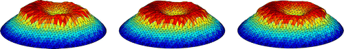
Figure 1. A free geodetic propagation with different Riemannian metrics. From top to bottom and left to right: Initial shape, Euclidiean, $H^0$-, $H^1$-, $H^2$-, $H^3$-, $H^5$- and $H^8$-metric.

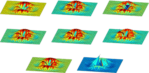
Figure 2. A shape together with the descent direction for different Riemannian metrics. From top to bottom and left to right: Euclidiean, $H^0$-, $H^1$- and $H^2$-metric.

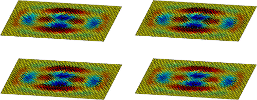
Figure 1 shows the final result of a free geodetic propagation using various Riemannian metrics. The following parameters were used in all cases: regularization $\mathit{\rho }=0$, number of steps along the geodesic $itereq=100$ and normalized step length $\mathit{\delta }=0.01$ (see Section 5.1 for explanation). The initial shape is the graph of the function defined in Equation (18(18) $$\begin{array}{c}\hfill g(x,y)=e^{\frac{1}{x^2-1}}{e}^{\frac{1}{y^2-1}}\left(cos,\left(10,\sqrt{{(x+.2)}^2+y^2}\right),+,cos,\left(10,\sqrt{{(x-.2)}^2+y^2}\right)\right).\end{array}$$(18) ); the initial ‘direction’ of the geodesic in the shape space is ${({\mathit{\kappa }}_p{n}_p)}_{p\in P}$ with$${\mathit{\kappa }}_p=e^{\frac{1}{|p_x|-1}}{e}^{\frac{1}{|p_y|-1}}.$$The result obtained with the Euclidean metric is locally quite smooth but contains self-intersections. With the different $H^n$-metrics, self-intersections in the process of deforming are more penalized for larger $n$ (strictly speaking only self-intersections which are due to the local contraction of several points to one point). Nevertheless, unnatural peaks may appear in the shape during the deformation process when using too large values for $n$, e.g. $n=8$.

Another example which describes the effects of the different metrics is given in Figure 2. Here, we consider the reconstruction of the shape defined in Equation (18(18) $$\begin{array}{c}\hfill g(x,y)=e^{\frac{1}{x^2-1}}{e}^{\frac{1}{y^2-1}}\left(cos,\left(10,\sqrt{{(x+.2)}^2+y^2}\right),+,cos,\left(10,\sqrt{{(x-.2)}^2+y^2}\right)\right).\end{array}$$(18) ). The current surface is the graph of the function $\overline{g}:[-1,1]\times [-1,1]\to \mathbb{R}$,$$\overline{g}(x,y)=\frac{1+{20|x|}^5}{10}{e}^{\frac{1}{x^2-1}}{e}^{\frac{1}{y^2-1}}\left(cos,\left(10,\sqrt{{(x+.2)}^2+y^2}\right),+,cos,\left(10,\sqrt{{(x-.2)}^2+y^2}\right)\right).$$We use $\mathit{\alpha }=0.05$ for the calculation of the optimal descent direction. The parameter $\mathit{\alpha }$ is the same as in Equation (14(14) $$\begin{array}{c}\hfill f(P):=\frac{1}{2}\sum _{p\in P}(⟨n_p(P),l⟩-s_p^{\ast }{)}^2+\frac{\mathit{\alpha }}{2}\sum _{(p,q)\in C}{\Vert n_p(P)-n_q(P)\Vert }^2\end{array}$$(14) ) and determines the regularization of the resulting shape. Obviously, the deformation vectors for the current shape are quite equally distributed over several regions if the Euclidean metric is employed. However, the deformation vectors are more concentrated to certain parts of the surface when using an $H^n$-metric; in particular, this is the case for larger $n$.

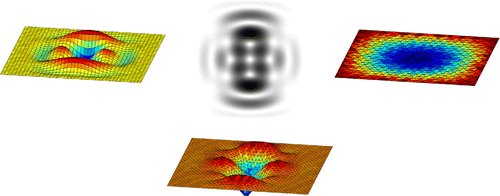
Figure 3. The synthetic shape, its shading image, the initial shape and its reconstruction using the SSD-method.

We discussed two algorithms, the GSD-method and the GNCG-method. Now, we have to find appropriate values for various parameter in the optimization algorithms; these values shall only depend on the shape which we want to reconstruct. We do this in order to compare the performance of the algorithms using different Riemannian metrics in the shape space $\mathcal{S}$; these metrics shall be the Euclidean metric, the $H^0$- and the $H^2$-metric. Below, we collect these values for each shape and discuss the advantages of these metrics in the different situations. In addition, we also present the reconstruction of the various surfaces using a standard variational approach. For this case, we use the functional $f$ from (14(14) $$\begin{array}{c}\hfill f(P):=\frac{1}{2}\sum _{p\in P}(⟨n_p(P),l⟩-s_p^{\ast }{)}^2+\frac{\mathit{\alpha }}{2}\sum _{(p,q)\in C}{\Vert n_p(P)-n_q(P)\Vert }^2\end{array}$$(14) ) which shall be minimized, but now we perform a standard steepest descent (SSD) with Armijo–Goldstein stepsize control. Consequently, we do not enforce the $N$ nodes of the surface to move along the local surface normal vectors, but instead we perform an unconstrained minimization process of $f$ w.r.t. all coordinates in ${\mathbb{R}}^{3N}$. Now, one also needs appropriate choices for the two parameters $\mathit{\sigma }$ and $\mathit{\mu }$ which appear in the Armijo-condition$$f(x+\mathit{\alpha }d)\le f(x)+\mathit{\alpha }\mathit{\sigma }\mathrm{\nabla }f{(x)}^{T}d$$and in the Goldstein-condition$$f(x+\mathit{\alpha }d)\ge f(x)+\mathit{\alpha }\mathit{\mu }\mathrm{\nabla }f{(x)}^{T}d.$$Typically, $\mathit{\sigma }$ and $\mathit{\mu }$ are chosen such that $0<\mathit{\sigma }<1/2<\mathit{\mu }<1$. We will give the values of $\mathit{\sigma }$ and $\mathit{\mu }$ below for each surface.

6.1 Synthetic surface

First, we consider a synthetic surface, which is the graph of the function $g:[-1,1]\times [-1,1]\to \mathbb{R}$,(18) $$\begin{array}{c}\hfill g(x,y)=e^{\frac{1}{x^2-1}}{e}^{\frac{1}{y^2-1}}\left(cos,\left(10,\sqrt{{(x+.2)}^2+y^2}\right),+,cos,\left(10,\sqrt{{(x-.2)}^2+y^2}\right)\right).\end{array}$$(18) This surface is shown in Figure 3. If the direction of the light coincides with the $z$-axis, we cannot initialize the algorithms with a triangulated planar surface since this is already a critical point of the function $f$ (see Equations (16(16) $$\begin{array}{c}\hfill \overrightarrow{\mathit{\kappa }}={\left(-,〈,(,\frac{\mathit{\partial }f}{\mathit{\partial }{r}^k},{)}_{k\in \{1,2,3\}},,,n_r,〉\right)}_{r\in P}\end{array}$$(16) ) and (17(17) $$\begin{array}{c}\hfill \overrightarrow{\mathit{\kappa }}=-U_{n,\mathit{\rho }}^{-1}(〈(\frac{\mathit{\partial }f}{\mathit{\partial }{r}^k}{)}_{k\in \{1,2,3\}},n_r〉{)}_{r\in P}.\end{array}$$(17) )). Hence, we use a triangulated mesh which slightly differs from a plane. Then, we reconstruct the shape in two steps. First, we use a coarse mesh (with edge length 0.1) to construct a shape which has the correct surface topography. If the resolution is too coarse, then we may not reconstruct all details of the topography; otherwise, if the resolution is too fine, the reconstruction is generally not smooth enough. An increase of the regularization term of $f$ is not the best choice since this also causes the final reconstruction to be overly smooth in comparison to the given data. However, this first optimization process results in a certain shape. Now, we refine the corresponding mesh and use this refined mesh (with edge length 0.05) as the initialization of the second optimization process on a finer level. This finer level is also the resolution which will be used for the reconstruction of the remaining shapes.

Figure 4. Reconstruction of the synthetic shape with the GSD-method using different Riemannian metrics. From left to right: Euclidean, $H^0$- and $H^2$-metric.

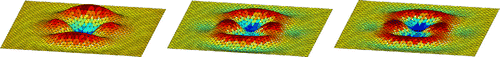
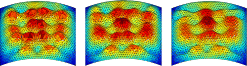
Figure 5. Reconstruction of the synthetic shape with the GNCG-method using different Riemannian metrics. From left to right: Euclidean, $H^0$- and $H^2$-metric.

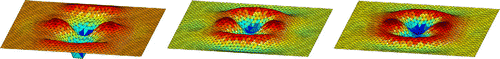
The Figures 4 and 5 show the final reconstruction of the surface for the three considered Riemannian metrics using the GSD-and the GNCG-method, respectively. If the $H^0$- or the $H^2$-metric is used, then the elevations in the reconstruction are more smoothly connected, in comparison to the Euclidean metric. Moreover, we see that the GNCG-algorithm together with the Euclidean metric does not converge to the underlying shape; however, if the $H^0$- or $H^2$-metric is used, then the algorithm does reconstruct the correct surface topography. Apart from the difference concerning the Euclidean metric, the GNCG-method generally results in a shape where elevations are a bit more suppressed than with the GSD-method. Figure 3 also shows the reconstruction when applying the SSD-method ($\mathit{\sigma }=0.25$, $\mathit{\mu }=0.9$). One immediately sees that the surface topography is not correctly reproduced, especially the first ‘valley’ seen from the observer does not appear at all. The results were obtained with the following choices for the parameters which we already described in Sections 5.1 and 5.2.

• light direction $l=(0,0,1)$, regularization $\mathit{\alpha }=0.05$,

• $\mathit{\rho }=0.0001$ for the $H^0$-metric and $\mathit{\rho }=1$ for the $H^2$-metric,

• $\mathtt{i}tereq=5$, $\mathtt{m}axit=30$, $\mathtt{d}elta=0.01$ and $\mathtt{r}estart=5$ for the first optimization process,

• $\mathtt{i}tereq=5$, $\mathtt{m}axit=20$, $\mathtt{d}elta=0.02$ and $\mathtt{r}estart=5$ for the second optimization process.

For the $H^2$-metric, a higher regularization is necessary as for the $H^0$-metric. This fact can also be seen from Equation (12(12) $$\begin{array}{c}\hfill \mathit{\rho }>{\mathit{\rho }}_0:=\underset{p\in P}{max}\sum _{q\in \mathcal{N}(p)\backslash \{p\}}\frac{1}{{\Vert p-q\Vert }^{2(n-1)}}.\end{array}$$(12) ), since the lower bound for the regularization, ${\mathit{\rho }}_0$, increases if the type $n$ of the $H^n$-metric increases.

In addition, we also apply the GSD-method together with the Euclidean metric to reconstruct the synthetic shape from the shading image of an oblique light source at $l=(0.1,0,1)$ and $l=(0,0.1,1)$. Strictly speaking, we use the normalized vector $\overline{l}=l/\Vert l\Vert$. For this case, we use exactly the same approach as for the reconstruction of the synthetic surface described above. The results are shown in Figure 6. For the case $l=(0.1,0,1)$, the algorithm is able to reconstruct the global topography of the surface but not with all details. Whereas the final shape obtained with a light source at $l=(0,0.1,1)$ is not even similar to the underlying shape.

Figure 6. Reconstruction of the synthetic shape using the GSD-method, the Euclidean metric and an oblique light source $l/\Vert l\Vert$. From left to right: $l=(0.1,0,1)$, $l=(0,0.1,1)$.

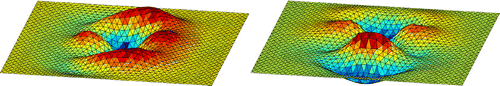
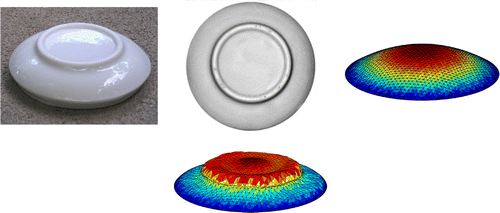
Figure 7. The bottom of the ceramic cup, its shading image, the initial shape and its reconstruction using the SSD-method.

6.2 Ceramic cup

The second shape is the bottom of a small ceramic cup. We use a grey-level image, which is a part of a usual jpg-image, to reconstruct the surface. However, the surface of the ceramic is also specular and thus some reflexions appear in the image. These reflexions are removed in the course of pre-processing the shading image. Figure 7 also shows the initial shape for the optimization algorithms, which is a flat parabolic surface. Here, we only use one resolution to reconstruct the surface. Figures 8 and 9 show the final result for the three different Riemannian metrics using the GSD- and GNCG-method. Here, we see that the $H^2$-metric, with both algorithms, yields a reconstructed surface which is considerably better than that for the Euclidean metric. First, the size of the triangles is much more homogeneous, and second, the circular elevation has nearly at all parts the same height, if the $H^2$-metric is used. Moreover, we see that the quality of the reconstruction – concerning rotational symmetry of the surface – is slightly better when applying the GSD-method. The result obtained by the SSD-method ($\mathit{\sigma }=0.01$, $\mathit{\mu }=0.1$) is shown in Figure 7. Here, it is necessary to choose smaller values for $\mathit{\sigma }$ and $\mathit{\mu }$; otherwise, the algorithm gets stuck in some local minima which are not close enough to the global one. At first glance, the surface is quite similar to the original one. But in contrast to the shape space optimization methods, the reconstructed surface is not the graph of a function. In principle, this is not an essential problem. However, it reveals an important advantage of the shape space optimization methods, namely the tendency to prevent singular triangles and regions with strongly deviating normal vectors. The choices for the parameters in the algorithms are

• light direction $l=(0,0,1)$, regularization $\mathit{\alpha }=0.1$,

• $\mathit{\rho }=0.001$ for the $H^0$-metric and $\mathit{\rho }=10$ for the $H^2$-metric,

• $\mathtt{i}tereq=5$, $\mathtt{m}axit=100$, $\mathtt{d}elta=0.02$ and $\mathtt{r}estart=5$ for the optimization process.

Figure 8. Reconstruction of the bottom of the ceramic cup with the GSD-method using different Riemannian metrics. From left to right: Euclidean, $H^0$- and $H^2$-metric.

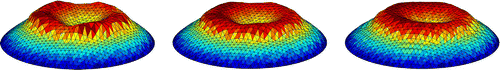
Figure 9. Reconstruction of the bottom of the ceramic cup with the GNCG-method using different Riemannian metrics. From left to right: Euclidean, $H^0$- and $H^2$-metric.

6.3 Face

A challenging problem is the reconstruction of a face from a shading image. Firstly, this is the case since a face consists of rather smooth parts together with regions where the local gradient is quite large. Secondly, some parts of the face may even not be visible, for example the side of the nose; strictly speaking, we therefore cannot consider the face as the graph of a function as explained in Section 4. And thirdly, a face is generally not an ideal Lambertian surface. Especially, the black eyebrow and eyelash have to be removed in the image; otherwise, the algorithms ‘interpret’ the eyelash as a region with a large gradient, in contrast to the reality. The initial shape for the reconstruction and the shading image of the face, where the eyebrow and eyelash are toned down, is shown in Figure10. However, neither the GSD-method nor the GNCG-method converges to a final shape which is sufficiently close to a face. Figures 11 and 12 contain the reconstruction of the face after 100 iterations. One immediately sees that several ‘balls’ emerge in the optimization process if the Euclidean or the $H^0$-metric are used. But this is not the case if one employs the $H^2$-metric, which smoothly connects the local maxima and minima of the surface. For the reconstruction of the face, the results obtained by the GSD- and GNCG-method hardly differ. The reconstruction of the face shown in Figure 10 using the SSD-method ($\mathit{\sigma }=0.25$, $\mathit{\mu }=0.9$) is in some sense similar to that of the ceramic cup. The surface also contains quite a sharp elevation at the boundary of the face itself. And the variation of the size of the triangles is considerably higher as for the shape space optimization methods. For the algorithms, we use

• light direction $l=(0,0,1)$, regularization $\mathit{\alpha }=0.1$,

• $\mathit{\rho }=0.0001$ for the $H^0$-metric and $\mathit{\rho }=1$ for the $H^2$-metric,

• $\mathtt{i}tereq=5$, $\mathtt{m}axit=100$, $\mathtt{d}elta=0.02$ and $\mathtt{r}estart=5$ for the optimization process.

Figure 10. The shading image of the face, the initial shape and its reconstruction using the SSD-method.

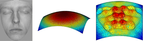
Figure 11. Reconstruction of the face with the GSD-method using different Riemannian metrics. From left to right: Euclidean, $H^0$- and $H^2$-metric.

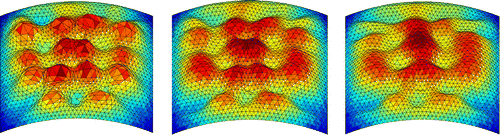
Figure 12. Reconstruction of the face with the GNCG-method using different Riemannian metrics. From left to right: Euclidean, $H^0$- and $H^2$-metric.

6.4 Quality measures and error estimation

In order to mathematically describe the quality of the reconstructed surfaces, one can define various functionals which return a small number for surfaces approximating the underlying shape quite well. For the synthetic surface – given by the function $g$ defined above – one may consider$$f_{\mathrm{shape}}(P):={\left(\sum _{p\in P},(,p_3,-,g,(p_1,p_2),{)}^2\right)}^{\frac{1}{2}}$$as such a quality measure, where $P\subset {\mathbb{R}}^3$ denotes the set of all nodes of the surface. This functional takes for each point $p\in P$ the difference between the $z$-component of $p$ and the value of $g$ at the projection of $p$ into the $xy$-plane into account. Since $f_{\mathrm{shape}}$ requires an explicit representation of the underlying surface as the graph of a function, we can apply it only to the synthetic shape. Another possible functional is given by$$f_{\mathrm{shade}}(P):={\left(\sum _{p\in P},(,⟨n_p(P),l⟩,-,s_p^{\ast },{)}^2\right)}^{\frac{1}{2}}$$which is essentially the data-fit term measuring differences between the prescribed shading values and that of the current surface. Below, we will present the evolution of $f_{\mathrm{shade}}$ during the process of reconstructing the ceramic cup. Finally, we may also use the functional $f$ itself as a natural quality measure since it includes both the adaptation of the shading values and a sufficient smoothness of the surface. We will use $f$ to visualize the progress of the reconstruction of the face.

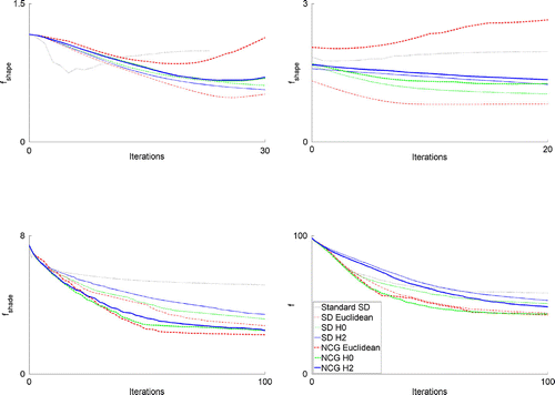
In Figure 13, there are four plots showing the behaviour of the above-introduced functionals in different situations. The upper left plot contains the evolution of $f_{\mathrm{shape}}$ for the coarse-grid optimization process of the synthetic shape, the upper right plot contains the same for the fine-grid optimization process. The lower left plot shows $f_{\mathrm{shade}}$ for the reconstruction of the ceramic cup and the lower right plot shows $f$ itself for the reconstruction of the face.

6.5 Performance of the SSD-method

Concerning the synthetic shape, it can be clearly seen from Figure 13 that the SSD-method reduces $f_{\mathrm{shape}}$ significantly faster than all the other methods within the first five iterations of the coarse-grid optimization. But from there on $f_{\mathrm{shape}}$ increases again and becomes nearly as large as at the beginning of the optimization process. But keep in mind that $f$ is the functional which is minimized by all the various methods, not $f_{\mathrm{shape}}$ or $f_{\mathrm{shade}}$. And since the SSD-method has approximately reached a local minimum of $f$ after 24 iterations (step-size smaller than ${10}^{-9}$), the algorithm terminates. The following fine-grid optimization process essentially cannot leave this local minimum and only refines the structure of the surface. This behaviour of the SSD-method also appears in a similar manner within the reconstruction of the ceramic cup and that of the face. At the beginning, $f_{\mathrm{shade}}$, respectively, $f$ decreases quite fast, but then the algorithm gets stuck in a local minimum. After 100 iterations, the SSD-method provides even the largest value of $f_{\mathrm{shade}}$ respectively $f$ amongst all the various methods.

Figure 13. Convergence of several optimization techniques in different situations. Top left: Synthetic shape (coarse-grid optimization). Top right: Synthetic shape (fine-grid optimization). Bottom left: Ceramic cup. Bottom right: Face. The legend applies to all four plots.

6.6 Comparison of the GSD-method, GNCG-method and various metrics

The performance of the two shape space optimization methods strongly depends on the problem. For the synthetic surface, the GSD-method always reaches a smaller value of $f_{\mathrm{shape}}$ than the GNCG-method – independent of the employed metric. Besides, we already pointed out that the surface is not correctly reconstructed when using the GNCG-method with the Euclidean metric; this fact is also shown in Figure 13. However, the best result is also obtained with the Euclidean metric, but together with the GSD-method. The situation is quite different for the reconstruction of the ceramic cup and the face. Here, the GNCG-method is able to minimize $f_{\mathrm{shade}}$, respectively, $f$ more efficiently. The smallest values of $f_{\mathrm{shade}}$ and $f$ are typically obtained when employing the Euclidean metric, followed by the $H^0$- and the $H^2$-metric. Nevertheless, the visual impression is somehow contrary since surfaces which have been reconstructed by using the $H^0$- or even $H^2$-metric are by far more smooth than surfaces for which the Euclidean metric has been used. We thus see that – independent of the optimization method – an appropriate choice of a Riemannian metric can direct the optimization process towards a desired class of surfaces in the shape space.

A further difference between the GSD- and the GNCG-method is the computational cost for the respective algorithms. The most expensive part of the GSD-method is the repeated evaluation of the right-hand side of the system of geodesic equations (line 9 of Algorithm 1). A similar computational effort is necessary to calculate the parallel translate of the previous search direction. Thus, the GNCG-method requires almost twice the numerical effort of the GSD-method. The costs for the various $H^n$-metrics are approximately the same but significantly higher as for the Euclidean metric, where the right-hand side of the geodesic equations is much simpler. Above, we have already seen that $H^n$-metrics with too large $n$, e.g. $n=8$, lead to unstable behaviour of the algorithms and to unnatural peaks in the reconstructed surface (see Figure 1). As in the situation of vector spaces, the GNCG-method is – on the one hand – able to minimize the objective functional more efficiently compared to the GSD-method. But, on the other hand, it has to be restarted with the optimal descent direction from time to time in order to obtain an efficient and stable algorithm.

7 Conclusion

In this paper, we presented two algorithms designed for optimization in a shape space of triangular meshes. These algorithms are the geodesic steepest descent (GSD) and the geodesic nonlinear conjugate gradient (GNCG) method, which are essentially the same as their non-geodesic counterparts apart from the fact that we now take steps along geodesics instead of straight lines. But the geodesics themselves depend on the Riemannian metric which is used in the shape space. Consequently, the performance of the two algorithms also depends on the employed Riemannian metric.

In Section 6, we described with several examples basic properties of various metrics as well as the GSD- and the GNCG-method. We showed that, in most cases, the geodesic optimization algorithms outperform the standard steepest descent (SSD) method (see Figure13). In addition, the reconstructed surfaces are generally more smooth in comparison to the SSD-method when applying a geodesic optimization method. Depending on the underlying surface, the GSD- or the GNCG-method is more advantageous (see the discussion at the end of Section 6). Generally, the reconstructed surfaces are more smooth if the shape space is endowed with some Hölder type $H^n$-metric and not with the standard Euclidean metric. Further advantages of $H^n$-metrics are the ability to prefer triangles which all have a similar size, and the tendency to smoothly connect elevations and depressions of a surface.

Compared to some methods presented in the reviews [14, 15] our approach does not give rise to sharp edges in the reconstructed surface. This is mainly a consequence of the regularization term within the objective functional, which penalizes differences between neighbouring surface normal vectors. Another feature of the strategy outlined in this article is the tendency to determine the global surface topography correctly (see the reconstruction of the synthetic surface and the ceramic cup). For surfaces with a more complex structure, this is often a problem (see [15] for another synthetic surface). The topography of the face is, nevertheless, not correctly reproduced also when applying our geodesic shape space methods. However, the freedom to choose an appropriate Riemannian metric in the shape space of triangular meshes makes it possible to adapt the optimization procedure to the structure of the underlying surface.

References

- Smith ST. Optimization techniques on Riemannian manifolds. In: Bloch A, editor. Hamiltonian and gradient flows, algorithms and control. Vol. 3, Fields institute communications. Providence (RI): American Mathematical Society; 1994. p. 113–136.
- Udrişte C. Convex functions and optimization methods on Riemannian manifolds. Vol. 297, Mathematics and its applications. Dordrecht: Kluwer Academic Publishers Group; 1994.
- Frankel T. The geometry of physics. An introduction. Cambridge (UK): Cambridge University Press; 2001.
- Michor P, Mumford D. An overview of the Riemannian metrics on spaces of curves using the Hamiltonian approach. Appl. Comput. Harmonic Anal. 2007;23:74–113.
- Kilian M, Mitra NJ, Pottmann H. Geometric modeling in shape space. ACM Trans. Graph. (Proc. SIGGRAPH’ 07). 2007;26:64.
- Schulz V. A Riemannian view on shape optimization. Forschungsbericht Universität Trier, Mathematik, Informatik. Report No.: 1; 2012.
- Ring W, Wirth B. Optimization methods on Riemannian manifolds and their application to shape space. SIAM J Optim. 2012;22:596–627.
- Nocedal J, Wright SJ. Numerical optimization. New York (NY): Springer; 2006.
- Jost J. Riemannian geometry and geometric analysis. Heidelberg: Springer; 2005.
- Amann H. Ordinary differential equations: an introduction to nonlinear analysis. Berlin: de Gruyter; 1990.
- Kniely M. Riemannian methods for optimization in shape space [master’s thesis]. Graz: Karl-Franzens-Universität; 2012.
- Horn B. Obtaining shape from shading information. In: Winston PH, editor. The psychology of computer vision. New York (NY): McGraw-Hill; 1975. Chapter 4; p. 115–155.
- Kimmel R. Numerical geometry of images. Theory, algorithms and applications. New York (NY): Springer; 2003.
- Zhang R, Tsai PS, Cryer J, Shah M. Shape from shading: a survey. IEEE Trans. Pattern Anal. Machine Intell. 1999;21:690–706.
- Durou JD, Falcone M, Sagona M. A survey of numerical methods for shape from shading. Rapport de recherche IRIT, Université Paul Sabatier. Report No.: 2004-2-R. Toulouse, France; 2004.
- LeVeque RJ. Numerical methods for conservation laws. Basel: Birkhäuser; 1992.