 ?Mathematical formulae have been encoded as MathML and are displayed in this HTML version using MathJax in order to improve their display. Uncheck the box to turn MathJax off. This feature requires Javascript. Click on a formula to zoom.
Abstract
In this paper, a concentration identification problem of the time fractional inhomogeneous diffusion equation (TFIDE) is investigated. The TFIDE is obtained from the classical diffusion equation by replacing the first-order time derivative by the Caputo fractional derivative of order . Our purpose is to recover the solute concentration from source measurement and boundary data. We show that this problem is severely ill-posed and further apply a convolution-type regularization method to solve it. Convergence estimates are given under a priori bound assumptions for the exact solution. Finally, we provide two numerical examples to confirm our theoretical analysis and show that the corresponding numerical method works effectively.
1. Introduction
In recent years, fractional calculus and fractional differential equations have been more and more extensively used in many scientific fields. For example, physical, chemical, biology, mechanical engineering, signal processing and systems identification, electrical, control theory, finance, fractional dynamics and so on, refer to [Citation1–Citation3]. As is known to all, in thermophysics, the normal diffusion obeys Fick (or Fourier) law:
where is diffusion flux,
is diffusion coefficient and
is concentration of substance. Moreover, the normal diffusion can be described quite well by classical diffusion equation (DE) which is derived from Fick law and, in probability theory, it corresponds to Brownian motion (BM). However, there are an increasing number of so-called anomalous diffusion arises in real world, such as the diffusion phenomena occurred in some media with memory and hereditary properties. The anomalous diffusion is not consistent with the classical Fick law, but satisfies what is called time fractional Fick law,[Citation4] i.e.
where is the Riemann–Liouville fractional derivative operator of order
defined by [Citation2]
(1)
(1)
where is Gamma function. Furthermore, if the function
is continuously differentiable and
, integration by parts leads to the Caputo fractional derivative of order
:
(2)
(2)
Then we get the Caputo time fractional Fick law:
This general Fick law derives the corresponding time fractional diffusion equation (TFDE), which arises by replacing the standard time partial derivative in the diffusion equation with a time fractional partial derivative and is closely related to fractional Brownian motion.[Citation5] The TFDE is gradually accepted as an important tool for describing anomalous diffusion.[Citation1, Citation6, Citation7] About the direct problems for TFDE, i.e. initial value problem and initial boundary value problem, which have been studied extensively in the past few years.[Citation8–Citation18] However, in some practical problems, the boundary data on the whole boundary cannot be obtained. We only know the noisy data on a part of the boundary or at some interior points of the concerned domain, which will lead to some inverse problems, i.e. fractional inverse diffusion problems (FIDP). For the results of FIDP, we can see [Citation19–Citation21]. However, in a practical application, not only does the boundary data need to measure, but also the source term (such as pollution source) need to measure. To the author’s knowledge, there is still not many results of inverse problems for source measurement.
In this article, we consider the following concentration identification problem (CIP) for the time fractional inhomogeneous diffusion equation (TFIDE):(3)
(3)
with the Cauchy condition and initial condition(4)
(4)
(5)
(5)
(6)
(6)
where is the solute concentration,
is the time-dependent source term and
denotes the solute concentration on left boundary. We will recover the solute concentration
in the region
from the measurement data of source term
and boundary concentration
. Here, we do not need the measurement data of diffusion flux on left boundary, which is different from the Cauchy data measurement in [Citation22]. In fact, it is difficult to measure diffusion flux directly in a practical application.
The CIP for the TFIDE is an inverse problem and is severely ill-posed (see Section 2). That means the solution does not depend continuously on the given data and any small error perturbation in the given data (such as the measurement data of source and boundary) may cause large change of the solution. In this paper, we will present a convolution-type regularization method which is proposed in [Citation23] to construct a stable approximate solution of CIP (Equation3(3)
(3) )–(Equation6
(6)
(6) ), which is a kind of modify equation method. Namely, we modify the Equation (Equation3
(3)
(3) ) as follows:
(7)
(7)
where ,
play a role of regularization parameter, and ‘
’ denotes convolution operation.
Our paper is divided into five sections. In Section 2, we explain the ill-posedness of the problem. In Section 3, we propose the regularization method and give some convergence estimates based on a priori assumptions for the exact solution. Numerical results are shown in Section 4. Finally, we give a conclusion in Section 5.
2. Ill-posedness of CIP and two relevant problems
To be able to apply the Fourier transform, we extend all the functions to the whole line by defining them to be zero for
. Here, and in the following sections,
denotes the
norm, i.e.
(8)
(8)
The Fourier transform of function is written as:
(9)
(9)
and the Laplace transform is defined by(10)
(10)
In addition, denotes the
norm, i.e.
(11)
(11)
By the initial condition , and applying the Laplace transform with respect to
in (Equation3
(3)
(3) )–(Equation5
(5)
(5) ), we get [Citation2]
(12)
(12)
(13)
(13)
(14)
(14)
Then the solution of (Equation8(8)
(8) )–(Equation10
(10)
(10) ) can easily be given by
(15)
(15)
Since and
are vanish for
, we find the Laplace transform and Fourier transform are related via
(16)
(16)
Then, from this relation and (Equation11(11)
(11) ), the solution of (Equation8
(8)
(8) )–(Equation10
(10)
(10) ) in frequency domain can be written as:
(17)
(17)
where(18)
(18)
and by (iii) in Lemma 3.1 (see Section 3)
Note that has a positive real part
, the small error given by
in the high-frequency components (
) will be amplified by the factor
(
). Moreover, the larger fraction order
is, the larger
is, then it causes the higher instability of solution of CIP and this will be reflected in our numerical results (see Section 4). Similarly, the error given by
will also be amplified by the factor
. Therefore, the CIP is severely ill-posed, we must use some regularization methods to deal with this problem.
Next, we will simply discuss two problems which are related to the CIP for TFIDE. The first one is time fractional homogeneous diffusion problem with non-zero Cauchy data:(19)
(19)
(20)
(20)
(21)
(21)
(22)
(22)
Similarly, we can use Laplace and Fourier transform and get its solution as follows:(23)
(23)
The second one is time fractional inhomogeneous diffusion problem with zero Cauchy data:(24)
(24)
(25)
(25)
(26)
(26)
(27)
(27)
Its solution is given by(28)
(28)
It is easy to see that the solution to the CIP (Equation3(3)
(3) )–(Equation6
(6)
(6) )
satisfy
. In order to obtain the convergence estimates of our regularization method, we first give the following a priori bound assumptions:
(29)
(29)
(30)
(30)
3. The regularization method and convergence estimates
In order to obtain a stable approximate solution of the CIP (Equation3(3)
(3) )–(Equation6
(6)
(6) ), we actually solve the following problem:
(31)
(31)
(32)
(32)
(33)
(33)
(34)
(34)
where is a regularization parameter, the measured data
and
satisfy
(35)
(35)
in which the constant is called a error level. We intend to recover the solute concentration
for
from the measured data
and
.
Similarly, by the integral transform method, we can obtain the formal solution of problem (Equation27(27)
(27) )–(Equation30
(30)
(30) ) as follows:
(36)
(36)
where(37)
(37)
Before the main theorems are given, we first prove some auxiliary lemmas.
Lemma 3.1
If ,
,
, then we have
(38)
(38)
(39)
(39)
(40)
(40)
Proof
About the proof of (i), we can see [Citation24] and (iii) is obvious.
(ii) Due to the proof is very similar to the one in [Citation22], we omit it.
Theorem 3.2
Assume that is the solution of problem (Equation3
(3)
(3) )–(Equation6
(6)
(6) ), whose Fourier transform is given by (Equation13
(13)
(13) ).
is the solution of problem (Equation27
(27)
(27) )–(Equation30
(30)
(30) ), whose Fourier transform is given by (Equation32
(32)
(32) ), and the measured data
,
satisfy (Equation31
(31)
(31) ).
| (1) | If the a priori bound (Equation25 | ||||
| (2) | If the a priori bound (Equation26 | ||||
Proof
(1) From (Equation19(19)
(19) ) and (Equation24
(24)
(24) ), we obtain
(45)
(45)
Thus, by (Equation13(13)
(13) ), (Equation25
(25)
(25) ), (Equation32
(32)
(32) ) and using the Parseval theorem, we have
where(46)
(46)
(47)
(47)
Next, we will estimate the four terms of (Equation42(42)
(42) ) and (Equation43
(43)
(43) ).
| (1) | Estimate of | ||||||||||||||||||||||
| (2) | Estimate of | ||||||||||||||||||||||
| (3) | Estimate of | ||||||||||||||||||||||
| (4) | Estimate of
| ||||||||||||||||||||||
Remark 3.3
In fact, we can first consider the two problems (Equation15(15)
(15) )–(Equation18
(18)
(18) ) and (Equation20
(20)
(20) )–(Equation23
(23)
(23) ), respectively, and then derive the convergence estimates of the CIP for the TFIDE, just like that in [Citation22]. But, for simplicity and uniformity, we directly deduce the convergence estimates from the CIP (Equation3
(3)
(3) ) to (Equation6
(6)
(6) ) itself.
Remark 3.4
Noting the -type regularization parameter choice rule (Equation37
(37)
(37) ) and the
-type choice rule (Equation39
(39)
(39) ), they also lead to the corresponding convergence estimates (
-type and
-type). Furthermore, above choice rules are independent of the fractional order
and space point
. But, in our numerical test (see Section 4), we see the fractional order and space point have big impacts on the numerical accuracy. Thus, the choice rules which depend on the fractional order
and space point
will be considered in our subsequent paper.
Remark 3.5
Since the regularization parameter choice rules (Equation37(37)
(37) ) and (Equation39
(39)
(39) ) contain the noise level
and a priori bounds, they are called a priori choice rule. But, in a practical application, the noise level and a priori bounds are usually not known, then a posteriori choice rules are popular. For details, refer to [Citation25]. Therefore, we will also consider some a posteriori choice rules in our future works.
4. Numerical examples
In this section, we present and discuss some numerical results obtained by the convolution-type regularization method for two examples. The convergence and stability of the algorithm when using noisy data can be verified. First, the implicit finite difference scheme (IFDS) is used to structure the source data and boundary data. Then, the finite difference solutions will be compared with the regularized solutions given by (Equation32(32)
(32) ).
We solve the following mixed boundary value problem by IFDS which is similar to the one in [Citation26](62)
(62)
(63)
(63)
(64)
(64)
(65)
(65)
where ,
are given boundary value and source function, respectively.
Denote the discrete points in the space interval as
,
with the space step size
and the grid points in the time interval
as
,
where
represents the time step size. Let
be the difference approximation to
. Then the difference scheme is given as follows:
(66)
(66)
and for ,
(67)
(67)
with boundary conditions(68)
(68)
and initial condition(69)
(69)
where and
,
Then the left boundary data (Equation4(4)
(4) ) are given by
(70)
(70)
Moreover, the following formulas are used to generate the noisy data(71)
(71)
(72)
(72)
where ,
,
and
are the exact data,
is a random number uniformly distributed in
and the magnitude
indicates a noise level. By using the noisy data
generated from (Equation67
(67)
(67) ) and (Equation68
(68)
(68) ), according to (Equation32
(32)
(32) ), we can get a regularized solution
computed using the Discrete Fourier Transform (DFT). In the numerical examples, we set the time step size
and the space step size
. For generating the noisy data, we use a noise level
. The source function is always given by
,
.
In order to test the accuracy of the regularized solution , we use the root mean square error defined as:
(73)
(73)
where is a fixed space point.
Example 1
(smooth example) Solve the direct problem (Equation58(58)
(58) )–(Equation61
(61)
(61) ) with
(74)
(74)
From (Equation13(13)
(13) ), (Equation19
(19)
(19) ), (Equation24
(24)
(24) ) and (Equation25
(25)
(25) ), we know
. However,
does not belong to
, so we can’t find the a priori bound
theoretically. But we will show that, by choosing the a priori bound
and getting the regularization parameter
from (Equation37
(37)
(37) ) at
, our method still produce a rational approximation. As for
, we obtain the regularization parameter
by trial and error. Then, we show the numerical results for
at
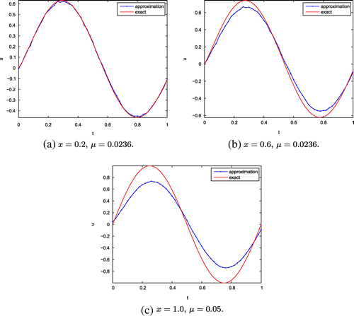
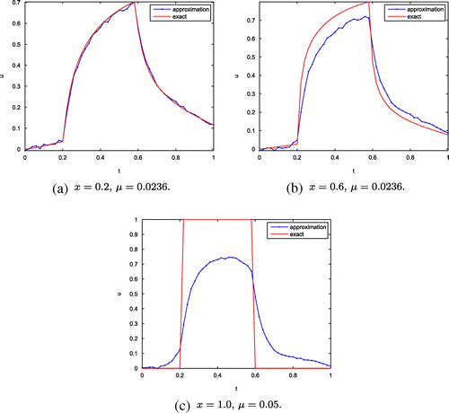
in Figure , for
at
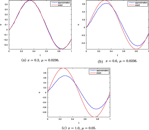
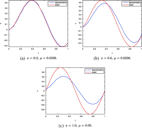
are shown in Figure and for
at
are shown in Figure . In Table , it illustrates the errors for these various values of fractional order
at different space point
.
Table 1. The errors for various values of fractional order
at various space point
, for Example 1.
Table 2. The errors for various values of fractional order
at various space point
, for Example 2.
Example 2
(nonsmooth example) In the direct problem (Equation58(58)
(58) )–(Equation61
(61)
(61) ), we set
(75)
(75)
where represents the Heaviside (unit step) function.
Although we can compute =
, the a priori bound
is still not given by
. So similar to Example 1, we also take
and obtain the regularization parameter
by (Equation37
(37)
(37) ) at
. By repeating experiment, we get the regularization parameter
at
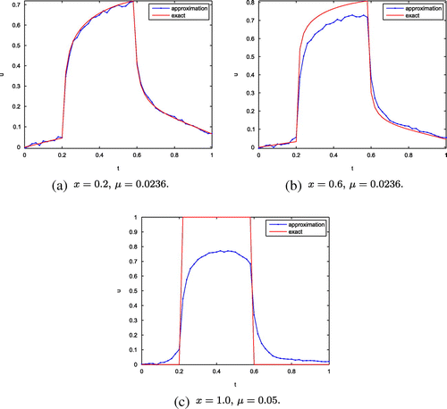
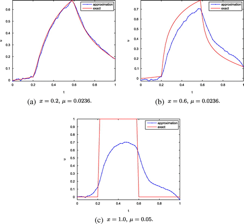
. Our method still has good computational effect. Then, we show the numerical results for
at
in Figure , for
at
are shown in Figure and for
at
are shown in Figure . Moreover, the errors
for these different fractional order at various space point
are presented in Table .
From Figures – and Tables and , it can be seen that numerical results near the boundary are better than the ones close to
. This is consistent with the convergence estimates (Equation38
(38)
(38) ) and (Equation40
(40)
(40) ). In particular, at
, (Equation40
(40)
(40) ) gives only
-type estimate which shows a slow convergence rate. Furthermore, we can see the numerical accuracy becomes worse as the order
of Caputo fractional derivative increases. In fact, as analysis in Section 2, we find the larger fractional order will cause higher instability of solution, and it is reflected naturally in the numerical results. Meanwhile, recalling the definition of
in IFDS (Equation62
(62)
(62) )–(Equation65
(65)
(65) ), it is easy to see that the factor
become singular as fractional order
approaches one. Namely, the IFDS cannot be used for classical diffusion equation (
). As for
, we should separately apply standard finite difference scheme (such as Crank-Nicolson scheme). Therefore, our numerical discussion only focus on the case
. In addition, we also find that the convolution-type regularization method applied in both Example 1 (smooth example) and Example 2 (non-smooth example) gives a similar degree of accuracy.
5. Conclusion
In this paper, a convolution-type regularization method is used to solve the CIP for the time fractional inhomogeneous diffusion equation in a strip domain. The convergence estimates have been presented for under a priori bound assumptions for the exact solution and the suitable choices of the regularization parameter. Finally, the numerical results illustrate our method is effective.
Acknowledgements
The author would like to thank the referees for their very useful suggestions.
Notes
The work described in this paper was supported by the NSF of China (11301168) and Plan for the growth of young teachers of Hunan University (531107040658).
References
- Metzler R, Klafter J. The random walk’s guide to anomalous diffusion: a fractional dynamics approach. Phys. Rep. 2000;339:1–77.
- Podlubny I. Fractional differential equations: an introduction to fractional derivatives, fractional differential equations, to methods of their solution and some of their applications. Vol. 198, Mathematics in science and engineering. San Diego (CA): Academic Press; 1999.
- Scalas E, Gorenflo R, Mainardi F. Fractional calculus and continuous-time finance. Phys. A. 2000;284:376–384.
- Jiang X, Xu M, Qi H. The fractional diffusion model with an absorption term and modified Fick’s law for non-local transport processes. Nonlinear Anal. Real World Appl. 2010;11:262–269. Available from: http://dx.doi.org/10.1016/j.nonrwa.2008.10.057
- Nourdin I. Selected aspects of fractional Brownian motion. Vol. 4, Bocconi and springer series. Milan: Springer; 2012. Available from: http://dx.doi.org/10.1007/978-88-470-2823-4
- Benson DA, Wheatcraft SW, Meerschaert MM. The fractional-order governing equation of Lévy motion. Water Resour. Res. 2000;36:1413–1423.
- Sokolov IM, Klafter J. From diffusion to anomalous diffusion: a century after Einstein’s Brownian motion. Chaos. 2005;15:1–7.
- Li XC, Xu MY, Jiang XY. Homotopy perturbation method to time-fractional diffusion equation with a moving boundary condition. Appl. Math. Comput. 2009;208:434–439.
- Scherer R, Kalla SL, Boyadjiev L, Al-Saqabi B. Numerical treatment of fractional heat equations. Appl. Numer. Math. 2008;58:1212–1223.
- Zhang P, Liu F. Implicit difference approximation for the time fractional diffusion equation. J. Appl. Math. Comput. 2006;22:87–99.
- Lin YM, Xu CJ. Finite difference/spectral approximations for the time-fractional diffusion equation. J. Comput. Phys. 2007;225:1533–1552.
- Shen S, Liu F, Anh V, Turner I. Detailed analysis of a conservative difference approximation for the time fractional diffusion equation. J. Appl. Math. Comput. 2006;22:1–19.
- Wyss W. The fractional diffusion equation. J. Math. Phys. 1986;27:2782–2785.
- Metzler R, Klafter J. Boundary value problems for fractional diffusion equations. Phys. A. 2000;278:107–125.
- Gorenflo R, Mainardi F. Some recent advances in theory and simulation of fractional diffusion processes. J. Comput. Appl. Math. 2009;229:400–415.
- Zhang Y, Meerschaert MM, Baeumer B. Particle tracking for time-fractional diffusion. Phys. Rev. E. 2008;78:1–7.
- Mainardi F, Pagnini G, Saxena RK. Fox H functions in fractional diffusion. J. Comput. Appl. Math. 2005;178:321–331.
- Mainardi F, Pagnini G, Gorenflo R. Some aspects of fractional diffusion equations of single and distributed order. Appl. Math. Comput. 2007;187:295–305.
- Murio DA. Time fractional IHCP with Caputo fractional derivatives. Comput. Math. Appl. 2008;56:2371–2381.
- Murio DA. Stable numerical solution of a fractional-diffusion inverse heat conduction problem. Comput. Math. Appl. 2007;53:1492–1501.
- Murio DA. Stable numerical evaluation of Grünwald–Letnikov fractional derivatives applied to a fractional ihcp. Inverse Probl. Sci. Eng. 2009;17:229–243.
- Zheng GH, Wei T. A new regularization method for a Cauchy problem of the time fractional diffusion equation. Adv. Comput. Math. 2012;36:377–398. Available from: http://dx.doi.org/10.1007/s10444-011-9206-3
- Zheng GH, Wei T. Two regularization methods for solving a Riesz–Feller space-fractional backward diffusion problem. Inverse Probl. 2010;26:115017, 22. Available from: http://dx.doi.org/10.1088/0266-5611/26/11/115017
- Qian Z, Fu CL. Regularization strategies for a two-dimensional inverse heat conduction problem. Inverse Probl. 2007;23:1053–1068.
- Engl HW, Hanke M, Neubauer A. Regularization of inverse problems. Vol. 375, Mathematics and its applications. Dordrecht: Kluwer Academic Publishers Group; 1996. Available from: http://dx.doi.org/10.1007/978-94-009-1740-8
- Murio DA. Implicit finite difference approximation for time fractional diffusion equations. Comput. Math. Appl. 2008;56:1138–1145.

