Approximation of mild solutions of the linear and nonlinear elliptic equations

Abstract

In this paper, we investigate the Cauchy problem for both linear and semi-linear elliptic equations. In general, the equations have the form$$\frac{{\mathit{\partial }}^2}{\mathit{\partial }{t}^2}u\left(t\right)=\mathcal{A}u\left(t\right)+f\left(t,,,u,\left(t\right)\right),t\in \left[0,,,T\right],$$

where $\mathcal{A}$ is a positive-definite, self-adjoint operator with compact inverse. As we know, these problems are well known to be ill-posed. On account of the orthonormal eigenbasis and the corresponding eigenvalues related to the operator, the method of separation of variables is used to give the solution in series representation. Thereby, we propose a modified method and show error estimations in many accepted cases. For illustration, two numerical examples, a modified Helmholtz equation and an elliptic sine-Gordon equation, are constructed to demonstrate the feasibility and efficiency of the proposed method.

Keywords:

• elliptic equation
• Cauchy problem
• ill-posed problem
• regularization method
• contraction principle

AMS Subject Classifications:

• 35K05
• 35K99
• 47J06
• 47H10x

1. Introduction

In practice, the Cauchy problem of elliptic equation arises in many applications. For example, in optoelectronics, the determination of a radiation field surrounding a source of radiation (e.g. a light emitting diode) is a frequently occurring problem. As a rule, experimental determination of the whole radiation field is not possible. Practically, we are able to measure the electromagnetic field only on some subset of physical space (e.g. on some surfaces). So, the problem arises how to reconstruct the radiation field from such experimental data (see for instance [1]). Other applications are in inverse obstacle problems (cf. [2]), in connection with inclusion detection by electrical impedance tomography when only one pair of boundary current and voltage is used for probing the examined body.[3]

Let $\mathcal{H}$ be a real Hilbert space, and let $\mathcal{A}:\mathcal{D}\left(\mathcal{A}\right)\subset \mathcal{H}\to \mathcal{H}$ be a positive-definite, self-adjoint operator with compact inverse on $\mathcal{H}$. In this paper, we consider the problem of finding a function $u:\left[0,,,T\right]\to \mathcal{H}$ satisfying(1) $$\begin{array}{c}\hfill \frac{{\mathit{\partial }}^2}{\mathit{\partial }{t}^2}u\left(t\right)=\mathcal{A}u\left(t\right)+f\left(t,,,u,\left(t\right)\right),t\in \left[0,,,T\right],\end{array}$$(1)

associated with the initial conditions(2) $$\begin{array}{c}\hfill u\left(0\right)=\mathit{\phi },\frac{\mathit{\partial }}{\mathit{\partial }t}u\left(0\right)=g,\end{array}$$(2)

where $f$ is a mapping from $\left[0,,,T\right]\times \mathcal{H}\to \mathcal{H}$, $\mathit{\phi }$ and $g$ are the exact data in $\mathcal{H}$. Physically, the exact data can only be measured, there will be measurement errors and we, thus, would have as data some functions ${\mathit{\phi }}^{\mathit{ϵ}}$ and $g^{\mathit{ϵ}}$ in $\mathcal{H}$ for which(3) $$\begin{array}{c}\hfill ∥\mathit{\phi },-,{\mathit{\phi }}^{\mathit{ϵ}}∥\le \mathit{ϵ},∥g,-,g^{\mathit{ϵ}}∥\le \mathit{ϵ},\end{array}$$(3)

where the constant $\mathit{ϵ}>0$ represents a bound on the measurement error and $∥.∥$ denotes the $\mathcal{H}$ norm.

Since Hadamard [4], it is well known that the Cauchy problem (1(1) $$\begin{array}{c}\hfill \frac{{\mathit{\partial }}^2}{\mathit{\partial }{t}^2}u\left(t\right)=\mathcal{A}u\left(t\right)+f\left(t,,,u,\left(t\right)\right),t\in \left[0,,,T\right],\end{array}$$(1) ) and (2(2) $$\begin{array}{c}\hfill u\left(0\right)=\mathit{\phi },\frac{\mathit{\partial }}{\mathit{\partial }t}u\left(0\right)=g,\end{array}$$(2) ) is severely ill-posed: although it has at most one solution, it may have none, and even if a solution exists, it does not depend continuously on the data $\mathit{\phi },g$ in any reasonable topology. Therefore, regularization is needed to stabilize the problem. In recent years, many special regularization methods for the homogeneous and nonhomogeneous Cauchy problem of elliptic equation have been proposed, such as Backus–Gilbert algorithm, [5] the method of wavelets,[6] quasi-reversibility method,[7] truncation method,[8] nonlocal boundary value method,[9] some other methods [10–13], etc.

Although we have many works on the linear homogeneous case of Cauchy problem for elliptic equations, regularization theory and numerical simulation for nonlinear elliptic equations are still limited. Especially, the nonlinear cases for elliptic equations appear in many real applications. For example, let us see a simple one inferred by taking $\mathcal{A}={\displaystyle \frac{-{\mathit{\partial }}^2}{\mathit{\partial }{x}^2}}$ and $\mathcal{D}\left(\mathcal{A}\right)=H_0^1\left(0,,,\mathit{\pi }\right)\subset \mathcal{H}=L^2\left(0,,,\mathit{\pi }\right)$ in the problem (1(1) $$\begin{array}{c}\hfill \frac{{\mathit{\partial }}^2}{\mathit{\partial }{t}^2}u\left(t\right)=\mathcal{A}u\left(t\right)+f\left(t,,,u,\left(t\right)\right),t\in \left[0,,,T\right],\end{array}$$(1) ) and (2(2) $$\begin{array}{c}\hfill u\left(0\right)=\mathit{\phi },\frac{\mathit{\partial }}{\mathit{\partial }t}u\left(0\right)=g,\end{array}$$(2) ). In particular, it is given by(4) $$\begin{array}{c}\hfill \frac{{\mathit{\partial }}^2}{\mathit{\partial }{t}^2}u\left(x,,,t\right)+\frac{{\mathit{\partial }}^2}{\mathit{\partial }{x}^2}u\left(x,,,t\right)=f\left(x,,,t,,,u,\left(x,,,t\right)\right),\left(x,,,t\right)\in \left(0,,,\mathit{\pi }\right)\times \left(0,,,1\right),\end{array}$$(4)

associated with the conditions$$u\left(0,,,t\right)=u\left(\mathit{\pi },,,t\right)=0,t\in \left(0,,,1\right),$$$$u\left(x,,,0\right)=\mathit{\phi }\left(x\right),\frac{\mathit{\partial }}{\mathit{\partial }t}u\left(x,,,0\right)=g\left(x\right),x\in \left(0,,,\mathit{\pi }\right).$$

If $f\left(x,,,t,,,u\right)=-k^{2}u$, then (4(4) $$\begin{array}{c}\hfill \frac{{\mathit{\partial }}^2}{\mathit{\partial }{t}^2}u\left(x,,,t\right)+\frac{{\mathit{\partial }}^2}{\mathit{\partial }{x}^2}u\left(x,,,t\right)=f\left(x,,,t,,,u,\left(x,,,t\right)\right),\left(x,,,t\right)\in \left(0,,,\mathit{\pi }\right)\times \left(0,,,1\right),\end{array}$$(4) ) is called the Helmholtz equation which has many applications related to wave propagation and vibration phenomena. If $f\left(x,,,t,,,u\right)=sinu$, then in (4(4) $$\begin{array}{c}\hfill \frac{{\mathit{\partial }}^2}{\mathit{\partial }{t}^2}u\left(x,,,t\right)+\frac{{\mathit{\partial }}^2}{\mathit{\partial }{x}^2}u\left(x,,,t\right)=f\left(x,,,t,,,u,\left(x,,,t\right)\right),\left(x,,,t\right)\in \left(0,,,\mathit{\pi }\right)\times \left(0,,,1\right),\end{array}$$(4) ) we obtain the elliptic sine-Gordon equation which occurs in several areas of mathematical physics including the theory of Josephson effects, superconductors and spin waves in ferromagnets, see e.g. [14]. If $f\left(x,,,t,,,u\right)=u-u^3$, we have the Allen-Cahn equation originally formulated in the description of bi-phase separation in fluids.

The operator $\mathcal{A}$ admits an orthonormal eigenbasis ${\left\{{\mathit{\varphi }}_p\right\}}_{p\ge 1}$ in $\mathcal{H}$, associated with the eigenvalues(5) $$\begin{array}{c}\hfill 0<{\mathit{\lambda }}_1\le {\mathit{\lambda }}_2\le ...\underset{p\to \infty }{lim}{\mathit{\lambda }}_p=\infty .\end{array}$$(5)

Let $u(t)=\sum _{p\ge 1}〈u,(t),,,{\mathit{\varphi }}_p〉{\mathit{\varphi }}_p$ be the Fourier series of $u$ in the Hilbert space $\mathcal{H}$. For the homogeneous problem, i.e. $f=0$ in (1(1) $$\begin{array}{c}\hfill \frac{{\mathit{\partial }}^2}{\mathit{\partial }{t}^2}u\left(t\right)=\mathcal{A}u\left(t\right)+f\left(t,,,u,\left(t\right)\right),t\in \left[0,,,T\right],\end{array}$$(1) ), we have(6) $$\begin{array}{cc}& \frac{d^2}{d{t}^2}〈u,(t),,,{\mathit{\varphi }}_p〉-{\mathit{\lambda }}_p〈u,(t),,,{\mathit{\varphi }}_p〉=0,\hfill \end{array}$$(6) (7) $$\begin{array}{cc}& 〈u,(0),,,{\mathit{\varphi }}_p〉=〈\mathit{\phi },,,{\mathit{\varphi }}_p〉,\frac{d}{dt}〈u,(0),,,{\mathit{\varphi }}_p〉=〈g,,,{\mathit{\varphi }}_p〉.\hfill \end{array}$$(7)

The formal solution of problem (6(6) $$\begin{array}{cc}& \frac{d^2}{d{t}^2}〈u,(t),,,{\mathit{\varphi }}_p〉-{\mathit{\lambda }}_p〈u,(t),,,{\mathit{\varphi }}_p〉=0,\hfill \end{array}$$(6) ) and (7(7) $$\begin{array}{cc}& 〈u,(0),,,{\mathit{\varphi }}_p〉=〈\mathit{\phi },,,{\mathit{\varphi }}_p〉,\frac{d}{dt}〈u,(0),,,{\mathit{\varphi }}_p〉=〈g,,,{\mathit{\varphi }}_p〉.\hfill \end{array}$$(7) ) is given by(8) $$\begin{array}{c}\hfill u(t)=\sum _{p=1}^{\infty }\left[cosh,\left(\sqrt{{\mathit{\lambda }}_p},t\right),〈\mathit{\phi },,,{\mathit{\varphi }}_p〉,+,\frac{sinh\left(\sqrt{{\mathit{\lambda }}_p},t\right)}{\sqrt{{\mathit{\lambda }}_p}},〈g,,,{\mathit{\varphi }}_p〉\right]{\mathit{\varphi }}_p.\end{array}$$(8)

On the other hand, for the inhomogeneous nonlinear problem (1(1) $$\begin{array}{c}\hfill \frac{{\mathit{\partial }}^2}{\mathit{\partial }{t}^2}u\left(t\right)=\mathcal{A}u\left(t\right)+f\left(t,,,u,\left(t\right)\right),t\in \left[0,,,T\right],\end{array}$$(1) ) and (2(2) $$\begin{array}{c}\hfill u\left(0\right)=\mathit{\phi },\frac{\mathit{\partial }}{\mathit{\partial }t}u\left(0\right)=g,\end{array}$$(2) ), we say that $u\in C([0,T];\mathcal{H})$ is a mild solution if $u$ satisfies the integral equation(9) $$\begin{array}{c}\hfill u(t)=\sum _{p=1}^{\infty }\left[,cosh,\left(\sqrt{{\mathit{\lambda }}_p},t\right),{\mathit{\phi }}_p,+,\frac{sinh\left(\sqrt{{\mathit{\lambda }}_p},t\right)}{\sqrt{{\mathit{\lambda }}_p}},g_p,+,\underset{0}{\overset{t}{\int }},\frac{sinh\left(\sqrt{{\mathit{\lambda }}_p},(t-s)\right)}{\sqrt{{\mathit{\lambda }}_p}},f_p,(u),(s),d,s,,\right]{\mathit{\varphi }}_p\end{array}$$(9)

where $f_p(u)(s)=〈f,(s,u(s)),,,{\mathit{\varphi }}_p,)〉$.

From now on, to regularize problem (1(1) $$\begin{array}{c}\hfill \frac{{\mathit{\partial }}^2}{\mathit{\partial }{t}^2}u\left(t\right)=\mathcal{A}u\left(t\right)+f\left(t,,,u,\left(t\right)\right),t\in \left[0,,,T\right],\end{array}$$(1) ) and (2(2) $$\begin{array}{c}\hfill u\left(0\right)=\mathit{\phi },\frac{\mathit{\partial }}{\mathit{\partial }t}u\left(0\right)=g,\end{array}$$(2) ), we only consider the integral Equation (9(9) $$\begin{array}{c}\hfill u(t)=\sum _{p=1}^{\infty }\left[,cosh,\left(\sqrt{{\mathit{\lambda }}_p},t\right),{\mathit{\phi }}_p,+,\frac{sinh\left(\sqrt{{\mathit{\lambda }}_p},t\right)}{\sqrt{{\mathit{\lambda }}_p}},g_p,+,\underset{0}{\overset{t}{\int }},\frac{sinh\left(\sqrt{{\mathit{\lambda }}_p},(t-s)\right)}{\sqrt{{\mathit{\lambda }}_p}},f_p,(u),(s),d,s,,\right]{\mathit{\varphi }}_p\end{array}$$(9) ) and find a regularization method for it. The main idea of integral equation method can be found in [15] on nonlinear backward heat equation.

The paper is organized as follows. In Section 2, we present our regularization method for the linear problem implied by letting $f=0$ in (1(1) $$\begin{array}{c}\hfill \frac{{\mathit{\partial }}^2}{\mathit{\partial }{t}^2}u\left(t\right)=\mathcal{A}u\left(t\right)+f\left(t,,,u,\left(t\right)\right),t\in \left[0,,,T\right],\end{array}$$(1) ). The theoretical results in the Section 2 are inspirable for us to suggest a new regularization method for the semi-linear case in Section 3. New convergence estimates are given under various a priori assumptions on the exact solution. Proofs of the results in these sections will be showed in the Appendix 1. In Section 4, simple numerical examples aimed to illustrate the main results of Section 3 are analysed.

2. The linear homogeneous problem

In [7], the authors applied the quasi-reversibility (QR) method to approximate problem (4(4) $$\begin{array}{c}\hfill \frac{{\mathit{\partial }}^2}{\mathit{\partial }{t}^2}u\left(x,,,t\right)+\frac{{\mathit{\partial }}^2}{\mathit{\partial }{x}^2}u\left(x,,,t\right)=f\left(x,,,t,,,u,\left(x,,,t\right)\right),\left(x,,,t\right)\in \left(0,,,\mathit{\pi }\right)\times \left(0,,,1\right),\end{array}$$(4) ) in the case $f=0$ and $g=0$. The main idea of the original QR method [16] is to approach the ill-posed Second-order Cauchy problem by a family of well-posed fourth-order problems depending on a (small) regularization parameter $\mathit{\beta }$. In particular, they considered the approximate problem(10) $$\begin{array}{c}\hfill \left\{\begin{array}{cc}{u}_{tt}^{\mathit{ϵ}}\left(x,,,t\right)+u_{xx}^{\mathit{ϵ}}\left(x,,,t\right)-{\mathit{\beta }}^2{u}_{ttxx}^{\mathit{ϵ}}\left(x,,,t\right)=0,\hfill & \left(x,,,t\right)\in \left(0,,,\mathit{\pi }\right)\times \left(0,,,1\right),\hfill \\ u\left(0,,,t\right)=u\left(\mathit{\pi },,,t\right)=0,\hfill & t\in \left(0,,,1\right),\hfill \\ u\left(x,,,0\right)={\mathit{\phi }}^{\mathit{ϵ}}\left(x\right),\frac{\mathit{\partial }}{\mathit{\partial }t}u\left(x,,,0\right)=0,\hfill & x\in \left(0,,,\mathit{\pi }\right).\hfill \end{array}\right.\end{array}$$(10)

The solution of (10(10) $$\begin{array}{c}\hfill \left\{\begin{array}{cc}{u}_{tt}^{\mathit{ϵ}}\left(x,,,t\right)+u_{xx}^{\mathit{ϵ}}\left(x,,,t\right)-{\mathit{\beta }}^2{u}_{ttxx}^{\mathit{ϵ}}\left(x,,,t\right)=0,\hfill & \left(x,,,t\right)\in \left(0,,,\mathit{\pi }\right)\times \left(0,,,1\right),\hfill \\ u\left(0,,,t\right)=u\left(\mathit{\pi },,,t\right)=0,\hfill & t\in \left(0,,,1\right),\hfill \\ u\left(x,,,0\right)={\mathit{\phi }}^{\mathit{ϵ}}\left(x\right),\frac{\mathit{\partial }}{\mathit{\partial }t}u\left(x,,,0\right)=0,\hfill & x\in \left(0,,,\mathit{\pi }\right).\hfill \end{array}\right.\end{array}$$(10) ) is given by(11) $$\begin{array}{c}\hfill u^{\mathit{ϵ}}(x,t)=\sum _{p=1}^{\infty }cosh\left(\frac{pt}{\sqrt{1+{\mathit{\beta }}^2{p}^2}}\right)〈{\mathit{\phi }}^{\mathit{ϵ}},(x),,,sin,(px)〉sin(px)\end{array}$$(11)

and the authors of [7] proved that $u^{\mathit{ϵ}}$ converges to the solution $u$ of homogeneous problem as $\mathit{ϵ}\to 0$.

Recently, the homogeneous problem has also been considered by Hao et al. [9]. They applied the method of non-local boundary value problems (also called quasi-boundary value method) to regularize the Cauchy problem (1(1) $$\begin{array}{c}\hfill \frac{{\mathit{\partial }}^2}{\mathit{\partial }{t}^2}u\left(t\right)=\mathcal{A}u\left(t\right)+f\left(t,,,u,\left(t\right)\right),t\in \left[0,,,T\right],\end{array}$$(1) ) and (2(2) $$\begin{array}{c}\hfill u\left(0\right)=\mathit{\phi },\frac{\mathit{\partial }}{\mathit{\partial }t}u\left(0\right)=g,\end{array}$$(2) ) with $g=0$ as follows(12) $$\begin{array}{c}\hfill \left\{\begin{array}{c}{u}_{tt}=\mathcal{A}u,\hfill \\ u_t(0)=0,\hfill \\ u(0)+\mathit{\beta }u(aT)=\mathit{\phi },\hfill \end{array}\right.\end{array}$$(12)

with $a\ge 1$ being given and $\mathit{\beta }>0$ is the regularization parameter. They proved that the solution to (12(12) $$\begin{array}{c}\hfill \left\{\begin{array}{c}{u}_{tt}=\mathcal{A}u,\hfill \\ u_t(0)=0,\hfill \\ u(0)+\mathit{\beta }u(aT)=\mathit{\phi },\hfill \end{array}\right.\end{array}$$(12) ) is(13) $$\begin{array}{c}\hfill u^{\mathit{\beta }}(t)=\sum _{p=1}^{\infty }\frac{cosh\left(\sqrt{{\mathit{\lambda }}_p},t\right)}{1+\mathit{\beta }cosh(a\sqrt{{\mathit{\lambda }}_p}t)}〈\mathit{\phi },{\mathit{\varphi }}_p〉{\mathit{\varphi }}_p\end{array}$$(13)

and $\Vert u^{\mathit{\beta }}(t)-u(t)\Vert \to 0$ as $\mathit{\beta }\to 0$ with some assumptions on the exact solution $u$.

Following the work,[9] in [8] Tuan et al. used a Fourier truncated method to treat the Cauchy problem (1(1) $$\begin{array}{c}\hfill \frac{{\mathit{\partial }}^2}{\mathit{\partial }{t}^2}u\left(t\right)=\mathcal{A}u\left(t\right)+f\left(t,,,u,\left(t\right)\right),t\in \left[0,,,T\right],\end{array}$$(1) ) and (2(2) $$\begin{array}{c}\hfill u\left(0\right)=\mathit{\phi },\frac{\mathit{\partial }}{\mathit{\partial }t}u\left(0\right)=g,\end{array}$$(2) ). From (8(8) $$\begin{array}{c}\hfill u(t)=\sum _{p=1}^{\infty }\left[cosh,\left(\sqrt{{\mathit{\lambda }}_p},t\right),〈\mathit{\phi },,,{\mathit{\varphi }}_p〉,+,\frac{sinh\left(\sqrt{{\mathit{\lambda }}_p},t\right)}{\sqrt{{\mathit{\lambda }}_p}},〈g,,,{\mathit{\varphi }}_p〉\right]{\mathit{\varphi }}_p.\end{array}$$(8) ), we observe that the data error can be arbitrarily amplified by the kernel $cosh\left(\sqrt{{\mathit{\lambda }}_p},t\right)$. That is the reason why the problem is ill-posed. Using the general regularization theory [17] and [7], we now give a more general principle of regularization methods for (8(8) $$\begin{array}{c}\hfill u(t)=\sum _{p=1}^{\infty }\left[cosh,\left(\sqrt{{\mathit{\lambda }}_p},t\right),〈\mathit{\phi },,,{\mathit{\varphi }}_p〉,+,\frac{sinh\left(\sqrt{{\mathit{\lambda }}_p},t\right)}{\sqrt{{\mathit{\lambda }}_p}},〈g,,,{\mathit{\varphi }}_p〉\right]{\mathit{\varphi }}_p.\end{array}$$(8) ). Our idea on regularization method is of constructing a new kernel $Q(t,{\mathit{\lambda }}_p,\mathit{\beta })$ and replacing $cosh\left(\sqrt{{\mathit{\lambda }}_p},t\right)$ by $Q(t,{\mathit{\lambda }}_p,\mathit{\beta })$, where the new kernel should satisfy

(A)	If $\mathit{\beta }$ is fixed, $Q(t,{\mathit{\lambda }}_p,\mathit{\beta })$ is bounded.
(B)	If $t,{\mathit{\lambda }}_p$ is fixed, then ${lim}_{\mathit{\beta }\to 0}Q(t,{\mathit{\lambda }}_p,\mathit{\beta })=cosh\left(\sqrt{{\mathit{\lambda }}_p},t\right)$.

The idea of properties (A) and (B) can be applied to other ill-posed problems when the solution has the similar form of (8(8) $$\begin{array}{c}\hfill u(t)=\sum _{p=1}^{\infty }\left[cosh,\left(\sqrt{{\mathit{\lambda }}_p},t\right),〈\mathit{\phi },,,{\mathit{\varphi }}_p〉,+,\frac{sinh\left(\sqrt{{\mathit{\lambda }}_p},t\right)}{\sqrt{{\mathit{\lambda }}_p}},〈g,,,{\mathit{\varphi }}_p〉\right]{\mathit{\varphi }}_p.\end{array}$$(8) ), e.g. the inverse heat conduction problem.[18] It is easy to check that the kernels $Q_1(t,{\mathit{\lambda }}_p,\mathit{\beta })=cosh\left(\frac{\sqrt{{\mathit{\lambda }}_p}t}{\sqrt{1+{\mathit{\beta }}^2{\mathit{\lambda }}_p}}\right)$ in [7] and $Q_2(t,{\mathit{\lambda }}_p,\mathit{\beta })=\frac{cosh\left(\sqrt{{\mathit{\lambda }}_p},t\right)}{1+\mathit{\beta }cosh(a\sqrt{{\mathit{\lambda }}_p}t)}$ in [9] satisfy (A) and (B).

To find a regularization solution for $u$, the instability terms $cosh\left(\sqrt{{\mathit{\lambda }}_p},t\right)$ and $sinh\left(\sqrt{{\mathit{\lambda }}_p},t\right)$ in (8(8) $$\begin{array}{c}\hfill u(t)=\sum _{p=1}^{\infty }\left[cosh,\left(\sqrt{{\mathit{\lambda }}_p},t\right),〈\mathit{\phi },,,{\mathit{\varphi }}_p〉,+,\frac{sinh\left(\sqrt{{\mathit{\lambda }}_p},t\right)}{\sqrt{{\mathit{\lambda }}_p}},〈g,,,{\mathit{\varphi }}_p〉\right]{\mathit{\varphi }}_p.\end{array}$$(8) ) should be replaced by two kernels $Q(t,{\mathit{\lambda }}_p,\mathit{\beta })$ and $R(t,{\mathit{\lambda }}_p,\mathit{\beta })$, respectively. Here, the kernel $Q$ satisfies (A), (B) and kernel $R$ satisfies the following conditions:

(C)	If $\mathit{\beta }$ is fixed, $R(t,{\mathit{\lambda }}_p,\mathit{\beta })$ is bounded.
(D)	If $t,{\mathit{\lambda }}_p$ are fixed, then ${lim}_{\mathit{\beta }\to 0}R(t,{\mathit{\lambda }}_p,\mathit{\beta })=sinh\left(\sqrt{{\mathit{\lambda }}_p},t\right)$.

In [8], we choose(14) $$\begin{array}{c}\hfill Q(t,{\mathit{\lambda }}_p,\mathit{\beta })=R(t,{\mathit{\lambda }}_p,\mathit{\beta })=\left\{\begin{array}{c}1,\text{if}{\mathit{\lambda }}_p\le m_{\mathit{\beta }}^2,\hfill \\ 0,\text{if}{\mathit{\lambda }}_p>m_{\mathit{\beta }}^2,\hfill \end{array}\right.\end{array}$$(14)

to get a truncation solution (see the formula (7) in p.2915, [8]), where $m_{\mathit{\beta }}$ satisfies ${lim}_{\mathit{\beta }\to +\infty }{m}_{\mathit{\beta }}=+\infty$. It is easy to check that $Q$ and $R$ defined in (14(14) $$\begin{array}{c}\hfill Q(t,{\mathit{\lambda }}_p,\mathit{\beta })=R(t,{\mathit{\lambda }}_p,\mathit{\beta })=\left\{\begin{array}{c}1,\text{if}{\mathit{\lambda }}_p\le m_{\mathit{\beta }}^2,\hfill \\ 0,\text{if}{\mathit{\lambda }}_p>m_{\mathit{\beta }}^2,\hfill \end{array}\right.\end{array}$$(14) ) satisfy $(A),(B)$ and $(C),(D)$, respectively.

In this section, we consider the homogeneous problem of (1(1) $$\begin{array}{c}\hfill \frac{{\mathit{\partial }}^2}{\mathit{\partial }{t}^2}u\left(t\right)=\mathcal{A}u\left(t\right)+f\left(t,,,u,\left(t\right)\right),t\in \left[0,,,T\right],\end{array}$$(1) ) (also given in [8]) by other choices for kernels. From the formula of $cosh\left(\sqrt{{\mathit{\lambda }}_p},t\right)$ and $sinh\left(\sqrt{{\mathit{\lambda }}_p},t\right)$, we realize that the term $e^{-\sqrt{{\mathit{\lambda }}_p}t}$ causes instability, while the term $e^{-\sqrt{{\mathit{\lambda }}_p}t}$ is stable being bounded by unity. Hence, we replace $cosh\left(\sqrt{{\mathit{\lambda }}_p},t\right)$ and $sinh\left(\sqrt{{\mathit{\lambda }}_p},t\right)$ by two new kernels$$\begin{array}{c}\hfill Q_3(t,{\mathit{\lambda }}_p,\mathit{\beta })={\displaystyle \frac{1}{2\mathit{\beta }+2e^{-\sqrt{{\mathit{\lambda }}_p}t}}}+\frac{e^{-\sqrt{{\mathit{\lambda }}_p}t}}{2},\end{array}$$

and$$\begin{array}{c}\hfill R(t,{\mathit{\lambda }}_p,\mathit{\beta })={\displaystyle \frac{1}{2\mathit{\beta }+2e^{-\sqrt{{\mathit{\lambda }}_p}t}}}-\frac{e^{-\sqrt{{\mathit{\lambda }}_p}t}}{2},\end{array}$$

to obtain an auxiliary regularized solution(15) $$\begin{array}{c}\hfill u^{\mathit{ϵ}}(t)=\sum _{p\ge 1}\left[Q,(t,{\mathit{\lambda }}_p,\mathit{\beta }),〈\mathit{\phi },,,{\mathit{\varphi }}_p〉,+,\frac{R(t,{\mathit{\lambda }}_p,\mathit{\beta })}{\sqrt{{\mathit{\lambda }}_p}},〈g,,,{\mathit{\varphi }}_p〉\right]{\mathit{\varphi }}_p.\end{array}$$(15)

Here and throughout the paper, $\mathit{\beta }=\mathit{\beta }\left(\mathit{ϵ}\right)$ is called the parameter regularization and satisfies ${\displaystyle {lim}_{\mathit{ϵ}\to 0}\mathit{\beta }\left(\mathit{ϵ}\right)=0}$. It is easy to check that $Q$ and $R$ satisfy $(A),(B)$ and $(C),(D)$, respectively. Moreover, (15(15) $$\begin{array}{c}\hfill u^{\mathit{ϵ}}(t)=\sum _{p\ge 1}\left[Q,(t,{\mathit{\lambda }}_p,\mathit{\beta }),〈\mathit{\phi },,,{\mathit{\varphi }}_p〉,+,\frac{R(t,{\mathit{\lambda }}_p,\mathit{\beta })}{\sqrt{{\mathit{\lambda }}_p}},〈g,,,{\mathit{\varphi }}_p〉\right]{\mathit{\varphi }}_p.\end{array}$$(15) ) leads to(16) $$\begin{array}{c}\hfill u^{\mathit{ϵ}}\left(t\right)=\sum _{p\ge 1}\left[{\displaystyle \frac{1}{2\mathit{\beta }+2e^{-\sqrt{{\mathit{\lambda }}_p}t}}},\left(〈\mathit{\phi },,,{\mathit{\varphi }}_p〉,+,\frac{〈g,,,{\mathit{\varphi }}_p〉}{\sqrt{{\mathit{\lambda }}_p}}\right),+,\frac{e^{-\sqrt{{\mathit{\lambda }}_p}t}}{2},\left(〈\mathit{\phi },,,{\mathit{\varphi }}_p〉,-,\frac{〈g,,,{\mathit{\varphi }}_p〉}{\sqrt{{\mathit{\lambda }}_p}}\right)\right]{\mathit{\varphi }}_p.\end{array}$$(16)

Under the inexact data ${\mathit{\phi }}^{\mathit{ϵ}}$ and $g^{\mathit{ϵ}}$, the regularized solution becomes(17) $$\begin{array}{c}\hfill v^{\mathit{ϵ}}\left(t\right)=\sum _{p\ge 1}\left[,{\displaystyle \frac{1}{2\mathit{\beta }+2e^{-\sqrt{{\mathit{\lambda }}_p}t}}},\left(,〈{\mathit{\phi }}^{\mathit{ϵ}},,,{\mathit{\varphi }}_p〉,+,\frac{〈g^{\mathit{ϵ}},,,{\mathit{\varphi }}_p〉}{\sqrt{{\mathit{\lambda }}_p}},\right),+,\frac{e^{-\sqrt{{\mathit{\lambda }}_p}t}}{2},\left(,〈{\mathit{\phi }}^{\mathit{ϵ}},,,{\mathit{\varphi }}_p〉,-,\frac{〈g^{\mathit{ϵ}},,,{\mathit{\varphi }}_p〉}{\sqrt{{\mathit{\lambda }}_p}},\right),\right]{\mathit{\varphi }}_p.\end{array}$$(17)

Remark 1

In the linear case of (1(1) $$\begin{array}{c}\hfill \frac{{\mathit{\partial }}^2}{\mathit{\partial }{t}^2}u\left(t\right)=\mathcal{A}u\left(t\right)+f\left(t,,,u,\left(t\right)\right),t\in \left[0,,,T\right],\end{array}$$(1) ), we denote the solution (8(8) $$\begin{array}{c}\hfill u(t)=\sum _{p=1}^{\infty }\left[cosh,\left(\sqrt{{\mathit{\lambda }}_p},t\right),〈\mathit{\phi },,,{\mathit{\varphi }}_p〉,+,\frac{sinh\left(\sqrt{{\mathit{\lambda }}_p},t\right)}{\sqrt{{\mathit{\lambda }}_p}},〈g,,,{\mathit{\varphi }}_p〉\right]{\mathit{\varphi }}_p.\end{array}$$(8) ) of (1(1) $$\begin{array}{c}\hfill \frac{{\mathit{\partial }}^2}{\mathit{\partial }{t}^2}u\left(t\right)=\mathcal{A}u\left(t\right)+f\left(t,,,u,\left(t\right)\right),t\in \left[0,,,T\right],\end{array}$$(1) ) and (2(2) $$\begin{array}{c}\hfill u\left(0\right)=\mathit{\phi },\frac{\mathit{\partial }}{\mathit{\partial }t}u\left(0\right)=g,\end{array}$$(2) ) by $u\left(t\right)$, the regularized solution (16(16) $$\begin{array}{c}\hfill u^{\mathit{ϵ}}\left(t\right)=\sum _{p\ge 1}\left[{\displaystyle \frac{1}{2\mathit{\beta }+2e^{-\sqrt{{\mathit{\lambda }}_p}t}}},\left(〈\mathit{\phi },,,{\mathit{\varphi }}_p〉,+,\frac{〈g,,,{\mathit{\varphi }}_p〉}{\sqrt{{\mathit{\lambda }}_p}}\right),+,\frac{e^{-\sqrt{{\mathit{\lambda }}_p}t}}{2},\left(〈\mathit{\phi },,,{\mathit{\varphi }}_p〉,-,\frac{〈g,,,{\mathit{\varphi }}_p〉}{\sqrt{{\mathit{\lambda }}_p}}\right)\right]{\mathit{\varphi }}_p.\end{array}$$(16) ) of (1(1) $$\begin{array}{c}\hfill \frac{{\mathit{\partial }}^2}{\mathit{\partial }{t}^2}u\left(t\right)=\mathcal{A}u\left(t\right)+f\left(t,,,u,\left(t\right)\right),t\in \left[0,,,T\right],\end{array}$$(1) ) and (2(2) $$\begin{array}{c}\hfill u\left(0\right)=\mathit{\phi },\frac{\mathit{\partial }}{\mathit{\partial }t}u\left(0\right)=g,\end{array}$$(2) ) by $u^{\mathit{ϵ}}\left(t\right)$ and the regularized solution (17(17) $$\begin{array}{c}\hfill v^{\mathit{ϵ}}\left(t\right)=\sum _{p\ge 1}\left[,{\displaystyle \frac{1}{2\mathit{\beta }+2e^{-\sqrt{{\mathit{\lambda }}_p}t}}},\left(,〈{\mathit{\phi }}^{\mathit{ϵ}},,,{\mathit{\varphi }}_p〉,+,\frac{〈g^{\mathit{ϵ}},,,{\mathit{\varphi }}_p〉}{\sqrt{{\mathit{\lambda }}_p}},\right),+,\frac{e^{-\sqrt{{\mathit{\lambda }}_p}t}}{2},\left(,〈{\mathit{\phi }}^{\mathit{ϵ}},,,{\mathit{\varphi }}_p〉,-,\frac{〈g^{\mathit{ϵ}},,,{\mathit{\varphi }}_p〉}{\sqrt{{\mathit{\lambda }}_p}},\right),\right]{\mathit{\varphi }}_p.\end{array}$$(17) ) of (1(1) $$\begin{array}{c}\hfill \frac{{\mathit{\partial }}^2}{\mathit{\partial }{t}^2}u\left(t\right)=\mathcal{A}u\left(t\right)+f\left(t,,,u,\left(t\right)\right),t\in \left[0,,,T\right],\end{array}$$(1) )–(3(3) $$\begin{array}{c}\hfill ∥\mathit{\phi },-,{\mathit{\phi }}^{\mathit{ϵ}}∥\le \mathit{ϵ},∥g,-,g^{\mathit{ϵ}}∥\le \mathit{ϵ},\end{array}$$(3) ) by $v^{\mathit{ϵ}}\left(t\right)$.

The main results of this section are in the following theorem.

Theorem 1

Let $\mathit{\beta }={\mathit{ϵ}}^m$ for some $m\in \left(0,,,1\right)$.

(i)	If there is a positive constant $E_1$ such that(18) $$\begin{array}{c}\hfill \sqrt{\frac{{∥u,\left(T\right)∥}^2}{2}+\frac{{∥{\displaystyle \frac{\mathit{\partial }}{\mathit{\partial }t}},u,\left(T\right)∥}^2}{2{\mathit{\lambda }}_1}}<E_1,\end{array}$$(18) then we have(19) $$\begin{array}{c}\hfill \left\{\begin{array}{cc}∥u,\left(t\right),-,v^{\mathit{ϵ}},\left(t\right)∥\le \sqrt{2\left(1,+,\frac{1}{{\mathit{\lambda }}_1}\right)}{\mathit{ϵ}}^{1-m}+E_1{\mathit{ϵ}}^m,\hfill & t\in \left[0,,,\frac{T}{2}\right],\hfill \\ ∥u,\left(t\right),-,v^{\mathit{ϵ}},\left(t\right)∥\le \sqrt{2\left(1,+,\frac{1}{{\mathit{\lambda }}_1}\right)}{\mathit{ϵ}}^{1-m}+E_1{\mathit{ϵ}}^{\frac{m\left(T,-,t\right)}{t}},\hfill & t\in \left[\frac{T}{2},,,T\right].\hfill \end{array}\right.\end{array}$$(19)
(ii)	If there is a positive constant $E_2$ such that(20) $$\begin{array}{c}\hfill \sqrt{\sum _{p\ge 1}{e}^{2\sqrt{{\mathit{\lambda }}_p}\left(T,-,t\right)}{\left(\sqrt{{\mathit{\lambda }}_p},〈u,\left(t\right),,,{\mathit{\varphi }}_p〉,+,〈{\displaystyle \frac{\mathit{\partial }}{\mathit{\partial }t}},u,\left(t\right),,,{\mathit{\varphi }}_p〉\right)}^2}<E_2,\end{array}$$(20) then we have(21) $$\begin{array}{c}\hfill \left\{\begin{array}{cc}∥u,\left(t\right),-,v^{\mathit{ϵ}},\left(t\right)∥\le \sqrt{2\left(1,+,\frac{1}{{\mathit{\lambda }}_1}\right)}{\mathit{ϵ}}^{1-m}+\frac{{\mathit{ϵ}}^m}{2\sqrt{{\mathit{\lambda }}_1}}{E}_2,\hfill & t\in \left[,0,,,\frac{T}{2},\right],\hfill \\ ∥u,\left(t\right),-,v^{\mathit{ϵ}},\left(t\right)∥\le \sqrt{2\left(1,+,\frac{1}{{\mathit{\lambda }}_1}\right)}{\mathit{ϵ}}^{1-m}+\frac{{\mathit{ϵ}}^{\frac{m\left(T,-,t\right)}{t}}}{2\sqrt{{\mathit{\lambda }}_1}}{\left[,\frac{{\mathit{\lambda }}_{1}T}{1+ln\left(\frac{\sqrt{{\mathit{\lambda }}_1}T}{{\mathit{ϵ}}^m}\right)},\right]}^{\frac{2t-T}{t}}{E}_2,\hfill & t\in \left[,\frac{T}{2},,,T,\right].\hfill \end{array}\right.\end{array}$$(21)
(iii)	If there is a positive constant $E_3$ such that(22) $$\begin{array}{c}\hfill \sqrt{\sum _{p\ge 1}{e}^{2\sqrt{{\mathit{\lambda }}_p}t}{\left(〈\sqrt{{\mathit{\lambda }}_p},u,\left(t\right),+,{\displaystyle \frac{\mathit{\partial }}{\mathit{\partial }t}},u,\left(t\right),,,{\mathit{\varphi }}_p〉\right)}^2}<E_3,\end{array}$$(22) then we have(23) $$\begin{array}{c}\hfill ∥u,\left(t\right),-,v^{\mathit{ϵ}},\left(t\right)∥\le \sqrt{2\left(1,+,\frac{1}{{\mathit{\lambda }}_1}\right)}{\mathit{ϵ}}^{1-m}+E_3\frac{{\mathit{ϵ}}^m}{2}.\end{array}$$(23)

In order to prove this theorem, we have to obtain some auxiliary results given by the lemmas below.

Lemma 1

Let $0<\mathit{\beta }<1$ and let $u^{\mathit{ϵ}}\left(t\right),v^{\mathit{ϵ}}\left(t\right)\in \mathcal{H}$ as introduced in Remark 1. Then, we have the following estimate(24) $$\begin{array}{c}\hfill ∥u^{\mathit{ϵ}},\left(t\right),-,v^{\mathit{ϵ}},\left(t\right)∥\le \sqrt{2\left(1,+,\frac{1}{{\mathit{\lambda }}_1}\right)}\mathit{ϵ}{\mathit{\beta }}^{-1}.\end{array}$$(24)

Lemma 2

Let $0<\mathit{\beta }<1$ and let $u\left(t\right),u^{\mathit{ϵ}}\left(t\right)\in \mathcal{H}$ as introduced in Remark 1. If (18(18) $$\begin{array}{c}\hfill \sqrt{\frac{{∥u,\left(T\right)∥}^2}{2}+\frac{{∥{\displaystyle \frac{\mathit{\partial }}{\mathit{\partial }t}},u,\left(T\right)∥}^2}{2{\mathit{\lambda }}_1}}<E_1,\end{array}$$(18) ) is satisfied, then we have the following estimate(25) $$\begin{array}{c}\hfill \left\{\begin{array}{cc}∥u,\left(t\right),-,u^{\mathit{ϵ}},\left(t\right)∥\le \mathit{\beta }{E}_1,\hfill & t\in \left[0,,,\frac{T}{2}\right],\hfill \\ ∥u,\left(t\right),-,u^{\mathit{ϵ}},\left(t\right)∥\le {\mathit{\beta }}^{\frac{T-t}{t}}{E}_1,\hfill & t\in \left[\frac{T}{2},,,T\right].\hfill \end{array}\right.\end{array}$$(25)

Lemma 3

Let $0<\mathit{\beta }<1$ and let $u\left(t\right),u^{\mathit{ϵ}}\left(t\right)\in \mathcal{H}$ as introduced in Remark 1. If (20(20) $$\begin{array}{c}\hfill \sqrt{\sum _{p\ge 1}{e}^{2\sqrt{{\mathit{\lambda }}_p}\left(T,-,t\right)}{\left(\sqrt{{\mathit{\lambda }}_p},〈u,\left(t\right),,,{\mathit{\varphi }}_p〉,+,〈{\displaystyle \frac{\mathit{\partial }}{\mathit{\partial }t}},u,\left(t\right),,,{\mathit{\varphi }}_p〉\right)}^2}<E_2,\end{array}$$(20) ) is satisfied, then we have the following estimate(26) $$\begin{array}{c}\hfill \left\{\begin{array}{cc}∥u,\left(t\right),-,u^{\mathit{ϵ}},\left(t\right)∥\le \frac{\mathit{\beta }}{2\sqrt{{\mathit{\lambda }}_1}}{E}_2,\hfill & t\in \left[0,,,\frac{T}{2}\right],\hfill \\ ∥u,\left(t\right),-,u^{\mathit{ϵ}},\left(t\right)∥\le \frac{1}{2\sqrt{{\mathit{\lambda }}_1}}{\mathit{\beta }}^{\frac{T-t}{t}}{E}_2,\hfill & t\in \left[\frac{T}{2},,,T\right].\hfill \end{array}\right.\end{array}$$(26)

Lemma 4

Let $0<\mathit{\beta }<1$ and let $u\left(t\right),u^{\mathit{ϵ}}\left(t\right)\in \mathcal{H}$ as introduced in Remark 1. If (22(22) $$\begin{array}{c}\hfill \sqrt{\sum _{p\ge 1}{e}^{2\sqrt{{\mathit{\lambda }}_p}t}{\left(〈\sqrt{{\mathit{\lambda }}_p},u,\left(t\right),+,{\displaystyle \frac{\mathit{\partial }}{\mathit{\partial }t}},u,\left(t\right),,,{\mathit{\varphi }}_p〉\right)}^2}<E_3,\end{array}$$(22) ) is satisfied, then we have the following estimate(27) $$\begin{array}{c}\hfill ∥u,\left(t\right),-,u^{\mathit{ϵ}},\left(t\right)∥\le \frac{\mathit{\beta }}{2}{E}_3.\end{array}$$(27)

Remark 2

At $t=T$, the error in case (i) is useless, while it is useful in case (ii). Moreover, in case (iii), under strong assumptions on $u$, we get the error of Holder-logarithmic type. In fact, if $\mathit{ϵ}$ is fixed then the right-hand side of (23(23) $$\begin{array}{c}\hfill ∥u,\left(t\right),-,v^{\mathit{ϵ}},\left(t\right)∥\le \sqrt{2\left(1,+,\frac{1}{{\mathit{\lambda }}_1}\right)}{\mathit{ϵ}}^{1-m}+E_3\frac{{\mathit{ϵ}}^m}{2}.\end{array}$$(23) ) attains its maximum value at $m={\displaystyle \frac{1}{2}}$. Thus, we obtain the error of order ${\mathit{ϵ}}^{\frac{1}{2}}$.

Remark 3

The condition in (20(20) $$\begin{array}{c}\hfill \sqrt{\sum _{p\ge 1}{e}^{2\sqrt{{\mathit{\lambda }}_p}\left(T,-,t\right)}{\left(\sqrt{{\mathit{\lambda }}_p},〈u,\left(t\right),,,{\mathit{\varphi }}_p〉,+,〈{\displaystyle \frac{\mathit{\partial }}{\mathit{\partial }t}},u,\left(t\right),,,{\mathit{\varphi }}_p〉\right)}^2}<E_2,\end{array}$$(20) ) can easily be satisfied. Indeed, we have that(28) $$\begin{array}{c}\hfill e^{\sqrt{{\mathit{\lambda }}_p}\left(T,-,t\right)}\left(\sqrt{{\mathit{\lambda }}_p},〈u,\left(t\right),,,{\mathit{\varphi }}_p〉,+,〈\frac{\mathit{\partial }}{\mathit{\partial }t},u,\left(t\right),,,{\mathit{\varphi }}_p〉\right)=\sqrt{{\mathit{\lambda }}_p}〈u,\left(T\right),,,{\mathit{\varphi }}_p〉+〈\frac{\mathit{\partial }}{\mathit{\partial }t},u,\left(T\right),,,{\mathit{\varphi }}_p〉,\end{array}$$(28)

and then the condition(29) $$\begin{array}{c}\hfill \sum _{p\ge 1}{\left(\sqrt{{\mathit{\lambda }}_p},〈u,\left(T\right),,,{\mathit{\varphi }}_p〉,+,〈\frac{\mathit{\partial }}{\mathit{\partial }t},u,\left(T\right),,,{\mathit{\varphi }}_p〉\right)}^2<\infty ,\end{array}$$(29)

is easy to check.

3. The semi-linear problem

In this section, we consider the problem (1(1) $$\begin{array}{c}\hfill \frac{{\mathit{\partial }}^2}{\mathit{\partial }{t}^2}u\left(t\right)=\mathcal{A}u\left(t\right)+f\left(t,,,u,\left(t\right)\right),t\in \left[0,,,T\right],\end{array}$$(1) ), where $f:\mathbb{R}\times \mathcal{H}\to \mathcal{H}$ is a Lipschitz continuous function, i.e. there exists $K>0$ independent of $w_1,w_2\in \mathcal{H},t\in \mathbb{R}$ such that(30) $$\begin{array}{c}\hfill ∥f,\left(t,,,w_1\right),-,f,\left(t,,,w_2\right)∥\le K∥w_1,-,w_2∥.\end{array}$$(30)

Since $0<t<s\le T$ , we know from (9(9) $$\begin{array}{c}\hfill u(t)=\sum _{p=1}^{\infty }\left[,cosh,\left(\sqrt{{\mathit{\lambda }}_p},t\right),{\mathit{\phi }}_p,+,\frac{sinh\left(\sqrt{{\mathit{\lambda }}_p},t\right)}{\sqrt{{\mathit{\lambda }}_p}},g_p,+,\underset{0}{\overset{t}{\int }},\frac{sinh\left(\sqrt{{\mathit{\lambda }}_p},(t-s)\right)}{\sqrt{{\mathit{\lambda }}_p}},f_p,(u),(s),d,s,,\right]{\mathit{\varphi }}_p\end{array}$$(9) ) that, when $p$ becomes large, the terms$$cosh\left(\sqrt{{\mathit{\lambda }}_p},t\right),sinh\left(\sqrt{{\mathit{\lambda }}_p},t\right),sinh\left(\sqrt{{\mathit{\lambda }}_p},(t-s)\right),$$

increase rather quickly. Thus, these terms cause instability. Hence, to find a regularized solution, we have to replace these terms by new kernels (called stability terms). These kernels have some common properties (A), (B), (C) and (D). In fact, we define the following regularized solution(31) $$\begin{array}{c}\hfill u^{\mathit{ϵ}}(t)=\sum _{p\ge 1}\left[P,(t,{\mathit{\lambda }}_p,\mathit{\beta }),{\mathit{\phi }}_p,+,\frac{Q(t,{\mathit{\lambda }}_p,\mathit{\beta })}{\sqrt{{\mathit{\lambda }}_p}},g_p,+,\underset{0}{\overset{t}{\int }},\frac{R(t,s,{\mathit{\lambda }}_p,\mathit{\beta })}{\sqrt{{\mathit{\lambda }}_p}},f_p,(u^{\mathit{ϵ}}),(s),d,s\right]{\mathit{\varphi }}_p,\end{array}$$(31)

analogous to (16(16) $$\begin{array}{c}\hfill u^{\mathit{ϵ}}\left(t\right)=\sum _{p\ge 1}\left[{\displaystyle \frac{1}{2\mathit{\beta }+2e^{-\sqrt{{\mathit{\lambda }}_p}t}}},\left(〈\mathit{\phi },,,{\mathit{\varphi }}_p〉,+,\frac{〈g,,,{\mathit{\varphi }}_p〉}{\sqrt{{\mathit{\lambda }}_p}}\right),+,\frac{e^{-\sqrt{{\mathit{\lambda }}_p}t}}{2},\left(〈\mathit{\phi },,,{\mathit{\varphi }}_p〉,-,\frac{〈g,,,{\mathit{\varphi }}_p〉}{\sqrt{{\mathit{\lambda }}_p}}\right)\right]{\mathit{\varphi }}_p.\end{array}$$(16) ). Here, $P(t,{\mathit{\lambda }}_p,\mathit{\beta }),Q(t,{\mathit{\lambda }}_p,\mathit{\beta })andR(t,s,{\mathit{\lambda }}_p,\mathit{\beta })$ are bounded by $C(\mathit{\beta })$ for any ${\mathit{\lambda }}_p>0$. Moreover, if $t,{\mathit{\lambda }}_p$ are fixed then$$\begin{array}{cc}& \underset{\mathit{\beta }\to 0}{lim}P(t,{\mathit{\lambda }}_p,\mathit{\beta })=cosh\left(\sqrt{{\mathit{\lambda }}_p},t\right),\underset{\mathit{\beta }\to 0}{lim}Q(t,{\mathit{\lambda }}_p,\mathit{\beta })=sinh\left(\sqrt{{\mathit{\lambda }}_p},t\right),\hfill \\ \hfill & \underset{\mathit{\beta }\to 0}{lim}R(t,s,{\mathit{\lambda }}_p,\mathit{\beta })=sinh\left(\sqrt{{\mathit{\lambda }}_p},(t-s)\right).\hfill \end{array}$$

We can give some assumptions for regularizing terms as follows:$$\begin{array}{cc}\hfill P(t,{\mathit{\lambda }}_p,\mathit{\beta })& =\frac{G({\mathit{\lambda }}_p,\mathit{\beta })e^{\sqrt{{\mathit{\lambda }}_p}t}+e^{-\sqrt{{\mathit{\lambda }}_p}t}}{2}\hfill \\ \hfill Q(t,{\mathit{\lambda }}_p,\mathit{\beta })& =\frac{G({\mathit{\lambda }}_p,\mathit{\beta })e^{\sqrt{{\mathit{\lambda }}_p}t}-e^{-\sqrt{{\mathit{\lambda }}_p}t}}{2}\hfill \\ \hfill R(t,s,{\mathit{\lambda }}_p,\mathit{\beta })& =\frac{G({\mathit{\lambda }}_p,\mathit{\beta })e^{\sqrt{{\mathit{\lambda }}_p}(t-s)}-e^{-\sqrt{{\mathit{\lambda }}_p}(t-s)}}{2},0\le s\le t.\hfill \\ \hfill \end{array}$$

Here $G$ satisfies$$\begin{array}{c}\hfill G({\mathit{\lambda }}_p,\mathit{\beta })e^{\sqrt{{\mathit{\lambda }}_p}t}\le {[M(\mathit{\beta })]}^{-\frac{t}{T}},\\ \hfill |G({\mathit{\lambda }}_p,\mathit{\beta })-1|e^{\sqrt{{\mathit{\lambda }}_p}(t-T)}\le {[M(\mathit{\beta })]}^{1-\frac{t}{T}},\end{array}$$

where ${lim}_{\mathit{\beta }\to 0}M(\mathit{\beta })=0$. In a future work, we will consider a general filter function method for the nonlinear problem.

For solving the problem in this paper, we take some suitable kernels as follows:$$\begin{array}{cc}\hfill P(t,{\mathit{\lambda }}_p,\mathit{\beta })& =\frac{e^{-\sqrt{{\mathit{\lambda }}_p}\left(T,-,t\right)}}{2\mathit{\beta }\sqrt{{\mathit{\lambda }}_p}+2e^{-\sqrt{{\mathit{\lambda }}_p}T}}+\frac{e^{-\sqrt{{\mathit{\lambda }}_p}t}}{2},\hfill \\ \hfill Q(t,{\mathit{\lambda }}_p,\mathit{\beta })& =\frac{e^{-\sqrt{{\mathit{\lambda }}_p}\left(T,-,t\right)}}{2\mathit{\beta }\sqrt{{\mathit{\lambda }}_p}+2e^{-\sqrt{{\mathit{\lambda }}_p}T}}-\frac{e^{-\sqrt{{\mathit{\lambda }}_p}t}}{2},\hfill \\ \hfill R(t,s,{\mathit{\lambda }}_p,\mathit{\beta })& =\frac{e^{-\sqrt{{\mathit{\lambda }}_p}\left(T,+,s,-,t\right)}}{2\mathit{\beta }\sqrt{{\mathit{\lambda }}_p}+2e^{-\sqrt{{\mathit{\lambda }}_p}T}}-\frac{e^{-\sqrt{{\mathit{\lambda }}_p}(t-s)}}{2}.\hfill \\ \hfill \end{array}$$

Then, we show error estimates between the solution $u\left(t\right)$ and the regularized solution $v^{\mathit{ϵ}}\left(t\right)$ in $\mathcal{H}$ norm under some supplementary error estimates and assumptions. Simultaneously, the uniqueness of solution $u^{\mathit{ϵ}},v^{\mathit{ϵ}}\in C\left(\left[0,,,T\right],;,\mathcal{H}\right)$ is proved by contraction principle.

Generally speaking, we obtain the following theorem.

Theorem 2

Let ${\displaystyle u\left(t\right)={\sum }_{p\ge 1}〈u,\left(t\right),,,{\mathit{\varphi }}_p〉{\mathit{\varphi }}_p}$ be the solution as denoted in (9(9) $$\begin{array}{c}\hfill u(t)=\sum _{p=1}^{\infty }\left[,cosh,\left(\sqrt{{\mathit{\lambda }}_p},t\right),{\mathit{\phi }}_p,+,\frac{sinh\left(\sqrt{{\mathit{\lambda }}_p},t\right)}{\sqrt{{\mathit{\lambda }}_p}},g_p,+,\underset{0}{\overset{t}{\int }},\frac{sinh\left(\sqrt{{\mathit{\lambda }}_p},(t-s)\right)}{\sqrt{{\mathit{\lambda }}_p}},f_p,(u),(s),d,s,,\right]{\mathit{\varphi }}_p\end{array}$$(9) ). Suppose there is a positive constant $P$ such that(32) $$\begin{array}{c}\hfill 4\underset{0\le t\le T}{sup}\sum _{p\ge 1}{e}^{\sqrt{{\mathit{\lambda }}_p}\left(T,-,t\right)}{\left(\sqrt{{\mathit{\lambda }}_p},〈u,\left(t\right),,,{\mathit{\varphi }}_p〉,+,〈\frac{\mathit{\partial }}{\mathit{\partial }t},u,\left(t\right),,,{\mathit{\varphi }}_p〉\right)}^2\le P.\end{array}$$(32)

Then by letting $\mathit{\beta }={\mathit{ϵ}}^m,m\in \left(0,,,1\right]$ the equation(33) $$\begin{array}{cc}\hfill v^{\mathit{ϵ}}\left(t\right)& =\sum _{p\ge 1}\left[\mathrm{\Phi },\left(\mathit{\beta },,,{\mathit{\lambda }}_p,,,t\right),{\mathcal{M}}_p,\left({\mathit{\phi }}^{\mathit{ϵ}},,,g^{\mathit{ϵ}}\right),+,{\int }_0^t,\mathrm{\Psi },\left(\mathit{\beta },,,{\mathit{\lambda }}_p,,,s,,,t\right),〈f,\left(s,,,v^{\mathit{ϵ}},\left(s\right)\right),,,{\mathit{\varphi }}_p〉,d,s\right]{\mathit{\varphi }}_p\hfill \\ \hfill & +\sum _{p\ge 1}\left[\frac{e^{-\sqrt{{\mathit{\lambda }}_p}t}}{2},{\mathcal{M}}_p,\left({\mathit{\phi }}^{\mathit{ϵ}},,,-,g^{\mathit{ϵ}}\right),-,{\int }_0^t,\frac{e^{\sqrt{{\mathit{\lambda }}_p}\left(s,-,t\right)}}{2\sqrt{{\mathit{\lambda }}_p}},〈f,\left(s,,,v^{\mathit{ϵ}},\left(s\right)\right),,,{\mathit{\varphi }}_p〉,d,s\right]{\mathit{\varphi }}_p,\hfill \end{array}$$(33)

has a unique solution $v^{\mathit{ϵ}}\in C\left(\left[0,,,T\right],;,\mathcal{H}\right)$ satisfying(34) $$\begin{array}{c}\hfill ∥u,\left(t\right),-,v^{\mathit{ϵ}},\left(t\right)∥\le Q{\mathit{ϵ}}^{\frac{m\left(T,-,t\right)}{T}}{T}^{\frac{t}{T}}{\left(ln,\left(\frac{T}{{\mathit{ϵ}}^m}\right)\right)}^{\frac{-t}{T}},\end{array}$$(34)

where, for each $p\ge 1$, ${\mathcal{M}}_p:\mathcal{H}\times \mathcal{H}\to \mathbb{R}$, is such that for $w_1,w_2\in \mathcal{H}$(35) $$\begin{array}{c}\hfill {\mathcal{M}}_p\left(w_1,,,w_2\right)=〈w_1,,,{\mathit{\varphi }}_p〉+\frac{〈w_2,,,{\mathit{\varphi }}_p〉}{\sqrt{{\mathit{\lambda }}_p}},\end{array}$$(35)

and(36) $$\begin{array}{cc}& \mathrm{\Phi }\left(\mathit{\beta },,,{\mathit{\lambda }}_p,,,t\right)=\frac{e^{-\sqrt{{\mathit{\lambda }}_p}\left(T,-,t\right)}}{2\mathit{\beta }\sqrt{{\mathit{\lambda }}_p}+2e^{-\sqrt{{\mathit{\lambda }}_p}T}},\mathrm{\Psi }\left(\mathit{\beta },,,{\mathit{\lambda }}_p,,,s,,,t\right)=\frac{e^{-\sqrt{{\mathit{\lambda }}_p}\left(T,+,s,-,t\right)}}{2\mathit{\beta }\sqrt{{\mathit{\lambda }}_p}+2\sqrt{{\mathit{\lambda }}_p}{e}^{-\sqrt{{\mathit{\lambda }}_p}T}},\hfill \end{array}$$(36) (37) $$\begin{array}{cc}& Q=\sqrt{\frac{3{\mathit{\lambda }}_1+3}{{\mathit{\lambda }}_1}}{e}^{\frac{3K^2{T}^{2}t}{2{\mathit{\lambda }}_1}}+e^{\frac{K^2{T}^{2}t}{2{\mathit{\lambda }}_1}}\sqrt{P}.\hfill \end{array}$$(37)

Remark 4

In above theorem, to obtain the error estimate (34(34) $$\begin{array}{c}\hfill ∥u,\left(t\right),-,v^{\mathit{ϵ}},\left(t\right)∥\le Q{\mathit{ϵ}}^{\frac{m\left(T,-,t\right)}{T}}{T}^{\frac{t}{T}}{\left(ln,\left(\frac{T}{{\mathit{ϵ}}^m}\right)\right)}^{\frac{-t}{T}},\end{array}$$(34) ), we require the strong priori assumption (32(32) $$\begin{array}{c}\hfill 4\underset{0\le t\le T}{sup}\sum _{p\ge 1}{e}^{\sqrt{{\mathit{\lambda }}_p}\left(T,-,t\right)}{\left(\sqrt{{\mathit{\lambda }}_p},〈u,\left(t\right),,,{\mathit{\varphi }}_p〉,+,〈\frac{\mathit{\partial }}{\mathit{\partial }t},u,\left(t\right),,,{\mathit{\varphi }}_p〉\right)}^2\le P.\end{array}$$(32) ). This is a weak point of this theorem. We are trying to remove this constraint in a future work.

The following lemmas will lead to proof of Theorem 2.

Lemma 5

Let $\mathrm{\Phi }\left(\mathit{\beta },,,{\mathit{\lambda }}_p,,,t\right)$ and $\mathrm{\Psi }\left(\mathit{\beta },,,{\mathit{\lambda }}_p,,,s,,,t\right)$ be defined as in (36(36) $$\begin{array}{cc}& \mathrm{\Phi }\left(\mathit{\beta },,,{\mathit{\lambda }}_p,,,t\right)=\frac{e^{-\sqrt{{\mathit{\lambda }}_p}\left(T,-,t\right)}}{2\mathit{\beta }\sqrt{{\mathit{\lambda }}_p}+2e^{-\sqrt{{\mathit{\lambda }}_p}T}},\mathrm{\Psi }\left(\mathit{\beta },,,{\mathit{\lambda }}_p,,,s,,,t\right)=\frac{e^{-\sqrt{{\mathit{\lambda }}_p}\left(T,+,s,-,t\right)}}{2\mathit{\beta }\sqrt{{\mathit{\lambda }}_p}+2\sqrt{{\mathit{\lambda }}_p}{e}^{-\sqrt{{\mathit{\lambda }}_p}T}},\hfill \end{array}$$(36) ). Then we have(38) $$\begin{array}{cc}& \mathrm{\Phi }\left(\mathit{\beta },,,{\mathit{\lambda }}_p,,,t\right)\le \frac{1}{2}{\left(\frac{\mathit{\beta }}{T}\right)}^{\frac{-t}{T}}{\left(ln,\left(\frac{T}{\mathit{\beta }}\right)\right)}^{\frac{-t}{T}},\hfill \end{array}$$(38) (39) $$\begin{array}{cc}& \mathrm{\Psi }\left(\mathit{\beta },,,{\mathit{\lambda }}_p,,,s,,,t\right)\le \frac{1}{2\sqrt{{\mathit{\lambda }}_1}}{\left(\frac{\mathit{\beta }}{T}\right)}^{\frac{s-t}{T}}{\left(ln,\left(\frac{T}{\mathit{\beta }}\right)\right)}^{\frac{s-t}{T}}.\hfill \end{array}$$(39)

Remark 5

The condition (32(32) $$\begin{array}{c}\hfill 4\underset{0\le t\le T}{sup}\sum _{p\ge 1}{e}^{\sqrt{{\mathit{\lambda }}_p}\left(T,-,t\right)}{\left(\sqrt{{\mathit{\lambda }}_p},〈u,\left(t\right),,,{\mathit{\varphi }}_p〉,+,〈\frac{\mathit{\partial }}{\mathit{\partial }t},u,\left(t\right),,,{\mathit{\varphi }}_p〉\right)}^2\le P.\end{array}$$(32) ) is similar to (20(20) $$\begin{array}{c}\hfill \sqrt{\sum _{p\ge 1}{e}^{2\sqrt{{\mathit{\lambda }}_p}\left(T,-,t\right)}{\left(\sqrt{{\mathit{\lambda }}_p},〈u,\left(t\right),,,{\mathit{\varphi }}_p〉,+,〈{\displaystyle \frac{\mathit{\partial }}{\mathit{\partial }t}},u,\left(t\right),,,{\mathit{\varphi }}_p〉\right)}^2}<E_2,\end{array}$$(20) ) and still questionable in practice. This is one of our limitation, but we hope that our theoretical assumptions on the exact solution may be relevant to some practical circumstances. The reader can see the numerical example 2, where the exact solution will cancel out the infinite sum in the assumptions.

Lemma 6

The integral Equation (33(33) $$\begin{array}{cc}\hfill v^{\mathit{ϵ}}\left(t\right)& =\sum _{p\ge 1}\left[\mathrm{\Phi },\left(\mathit{\beta },,,{\mathit{\lambda }}_p,,,t\right),{\mathcal{M}}_p,\left({\mathit{\phi }}^{\mathit{ϵ}},,,g^{\mathit{ϵ}}\right),+,{\int }_0^t,\mathrm{\Psi },\left(\mathit{\beta },,,{\mathit{\lambda }}_p,,,s,,,t\right),〈f,\left(s,,,v^{\mathit{ϵ}},\left(s\right)\right),,,{\mathit{\varphi }}_p〉,d,s\right]{\mathit{\varphi }}_p\hfill \\ \hfill & +\sum _{p\ge 1}\left[\frac{e^{-\sqrt{{\mathit{\lambda }}_p}t}}{2},{\mathcal{M}}_p,\left({\mathit{\phi }}^{\mathit{ϵ}},,,-,g^{\mathit{ϵ}}\right),-,{\int }_0^t,\frac{e^{\sqrt{{\mathit{\lambda }}_p}\left(s,-,t\right)}}{2\sqrt{{\mathit{\lambda }}_p}},〈f,\left(s,,,v^{\mathit{ϵ}},\left(s\right)\right),,,{\mathit{\varphi }}_p〉,d,s\right]{\mathit{\varphi }}_p,\hfill \end{array}$$(33) ) has a unique solution $v^{\mathit{ϵ}}\in C\left(\left[0,,,T\right],;,\mathcal{H}\right)$.

Lemma 7

The equation(40) $$\begin{array}{cc}\hfill u^{\mathit{ϵ}}\left(t\right)& =\sum _{p\ge 1}\left[\mathrm{\Phi },\left(\mathit{\beta },,,{\mathit{\lambda }}_p,,,t\right),{\mathcal{M}}_p,\left(\mathit{\phi },,,g\right),+,{\int }_0^t,\mathrm{\Psi },\left(\mathit{\beta },,,{\mathit{\lambda }}_p,,,s,,,t\right),〈f,\left(s,,,u^{\mathit{ϵ}},\left(s\right)\right),,,{\mathit{\varphi }}_p〉,d,s\right]{\mathit{\varphi }}_p\hfill \\ \hfill & +\sum _{p\ge 1}\left[\frac{e^{-\sqrt{{\mathit{\lambda }}_p}t}}{2},{\mathcal{M}}_p,\left(\mathit{\phi },,,-,g\right),-,{\int }_0^t,\frac{e^{\sqrt{{\mathit{\lambda }}_p}\left(s,-,t\right)}}{2\sqrt{{\mathit{\lambda }}_p}},〈f,\left(s,,,u^{\mathit{ϵ}},\left(s\right)\right),,,{\mathit{\varphi }}_p〉,d,s\right]{\mathit{\varphi }}_p,\hfill \end{array}$$(40)

has a unique solution $u^{\mathit{ϵ}}\in C\left(\left[0,,,T\right],;,\mathcal{H}\right)$ and the following error estimates hold:(41) $$\begin{array}{cc}& ∥v^{\mathit{ϵ}},\left(t\right),-,u^{\mathit{ϵ}},\left(t\right)∥\le \sqrt{\frac{3{\mathit{\lambda }}_1+3}{{\mathit{\lambda }}_1}}{e}^{\frac{3K^2{T}^{2}t}{2{\mathit{\lambda }}_1}}{\left(\frac{\mathit{\beta }}{T}\right)}^{\frac{-t}{T}}{\left(ln,\left(\frac{T}{\mathit{\beta }}\right)\right)}^{\frac{-t}{T}}\mathit{ϵ},\hfill \end{array}$$(41) (42) $$\begin{array}{cc}& ∥u,\left(t\right),-,u^{\mathit{ϵ}},\left(t\right)∥\le e^{\frac{T^2{K}^{2}t}{2{\mathit{\lambda }}_1}}\sqrt{P}\mathit{\beta }{\left(\frac{\mathit{\beta }}{T}\right)}^{\frac{-t}{T}}{\left(ln,\left(\frac{T}{\mathit{\beta }}\right)\right)}^{\frac{-t}{T}}.\hfill \end{array}$$(42)

4. Numerical examples

In this section, we show two numerical examples to validate the accuracy and efficiency of our proposed regularization method for 1-D semi-linear elliptic problems including both linear and nonlinear cases. The examples are with the operator $\mathcal{A}=-{\displaystyle \frac{{\mathit{\partial }}^2}{\mathit{\partial }{x}^2}}$ and taken in the Hilbert space $\mathcal{H}=L^2\left(0,,,\mathit{\pi }\right)$. Particularly, we give examples of a modified Helmholtz equation and an elliptic sine-Gordon equation to demonstrate how the method works.

We investigate the propagation of the error $\mathit{ϵ}={10}^{-r}$ for $r\in \mathbb{N}$. The couple of Cauchy $\left({\mathit{\phi }}^{\mathit{ϵ}},,,g^{\mathit{ϵ}}\right)$ are measured data containing random noise. More precisely, we take perturbations in the exact data $\left(\mathit{\phi },,,g\right)$ to define $\left({\mathit{\phi }}^{\mathit{ϵ}},,,g^{\mathit{ϵ}}\right)$ as$${\mathit{\phi }}^{\mathit{ϵ}}\left(x\right)=\mathit{\phi }\left(x\right)+\frac{\mathit{ϵ}·\text{rand}}{\sqrt{\mathit{\pi }}},g^{\mathit{ϵ}}\left(x\right)=g\left(x\right)+\frac{\mathit{ϵ}·\text{rand}}{\sqrt{\mathit{\pi }}},$$

where $\text{rand}$ is a random number in $\left[-,1,,,1\right]$.

Then, the regularized solution (choosing $m=0.99$) is expected to be closed to the exact solution under a proper discretization. For convergence tests, we introduce two errors: the absolute error at the midpoint ${\displaystyle \frac{\mathit{\pi }}{2}}$ and the relative root mean square (RRMS) error. Also, 2-D and 3-D graphs are plotted and analysed.

To be more coherent, we are going to divide this section into two subsections. The first one is to consider the modified Helmholtz equation and the second one is for the elliptic sine-Gordon equation.

Remark 6

Generally, the whole process is summarized in the following steps.

Step 1 Given $N,K_1$ and $M$ to have$$x_j=j\mathrm{\Delta }x,\mathrm{\Delta }x={\displaystyle \frac{1}{K_1}},j=\overline{0,K_1},t_i=i\mathrm{\Delta }t,\mathrm{\Delta }t={\displaystyle \frac{1}{M}},i=\overline{0,M}.$$Step 2 Choose $r$, put $v^{\mathit{ϵ}}\left(x,,,t_i\right)=v_i^{\mathit{ϵ}}\left(x\right),i=\overline{0,M}$ and set $v_0^{\mathit{ϵ}}\left(x\right)={\mathit{\phi }}^{\mathit{ϵ}}\left(x\right)$. Define$$V^{\mathit{ϵ}}\left(x\right)={\left[\begin{array}{cccc}{v}_0^{\mathit{ϵ}}\left(x\right)& v_1^{\mathit{ϵ}}\left(x\right)& ...& v_M^{\mathit{ϵ}}\left(x\right)\end{array}\right]}^{tr}\in {\mathbb{R}}^{M+1}.$$Step 3 For $i=\overline{0,M}$ and $j=\overline{0,K_1},$ put $v_i^{\mathit{ϵ}}\left(x_j\right)=v_{i,j}^{\mathit{ϵ}}$ and $u\left(x_j,,,t_i\right)=u_{ji}$, we find the matrices in ${\mathbb{R}}^{M+1}\times {\mathbb{R}}^{K_1+1}$ containing all discrete values of the exact solution $u\left(x,,,t\right)$ and the regularized solution $v^{\mathit{ϵ}}\left(x,,,t\right)$, denoted by $U$ and $V^{\mathit{ϵ}}$, respectively,$$U=\left[\begin{array}{cccc}{u}_{0,0}& u_{0,1}& \cdots & u_{0,K_1}\\ u_{1,0}& u_{1,1}& \cdots & u_{1,K_1}\\ ⋮& ⋮& \ddots & ⋮\\ u_{M,0}& u_{M,1}& \dots & u_{M,K_1}\end{array}\right],V^{\mathit{ϵ}}=\left[\begin{array}{cccc}{v}_{0,0}^{\mathit{ϵ}}& v_{0,1}^{\mathit{ϵ}}& \cdots & v_{0,K_1}^{\mathit{ϵ}}\\ v_{1,0}^{\mathit{ϵ}}& v_{1,1}^{\mathit{ϵ}}& \cdots & v_{1,K_1}^{\mathit{ϵ}}\\ ⋮& ⋮& \ddots & ⋮\\ v_{M,0}^{\mathit{ϵ}}& v_{M,1}^{\mathit{ϵ}}& \dots & v_{M,K_1}^{\mathit{ϵ}}\end{array}\right].$$Step 4 Calculate the errors and present 2-D and 3-D graphs:(43) $$\begin{array}{cc}& E\left(t_i\right)=\left|u,\left(\frac{\mathit{\pi }}{2},,,t_i\right),-,v^{\mathit{ϵ}},\left(\frac{\mathit{\pi }}{2},,,t_i\right)\right|,\hfill \end{array}$$(43) (44) $$\begin{array}{cc}& RRMS\left(t_i\right)=\frac{\sqrt{\sum _{0\le j\le K}{\left|u,\left(x_j,,,t_i\right),-,v^{\mathit{ϵ}},\left(x_j,,,t_i\right)\right|}^2}}{\sqrt{\sum _{0\le j\le K}{\left|u,\left(x_j,,,t_i\right)\right|}^2}}.\hfill \end{array}$$(44)

4.1. Example 1

We will consider the following Cauchy problem for the modified Helmholtz equation:(45) $$\begin{array}{c}\hfill \left\{\begin{array}{cc}\frac{{\mathit{\partial }}^2}{\mathit{\partial }{t}^2}u\left(x,,,t\right)+\frac{{\mathit{\partial }}^2}{\mathit{\partial }{x}^2}u\left(x,,,t\right)=u\left(x,,,t\right),\hfill & \left(x,,,t\right)\in \left(0,,,\mathit{\pi }\right)\times \left(0,,,1\right),\hfill \\ \frac{\mathit{\partial }}{\mathit{\partial }x}u\left(0,,,t\right)=u\left(\mathit{\pi },,,t\right)=0,\hfill & t\in \left(0,,,1\right),\hfill \\ u\left(x,,,0\right)=\mathit{\phi }\left(x\right),\frac{\mathit{\partial }}{\mathit{\partial }t}u\left(x,,,0\right)=0,\hfill & x\in \left(0,,,\mathit{\pi }\right).\hfill \end{array}\right.\end{array}$$(45)

Based on $\mathcal{D}\left(\mathcal{A}\right)=\left\{v,\in ,H^1,\left(0,,,\mathit{\pi }\right),:,v,\left(\mathit{\pi }\right),=,0\right\}$, we get an orthonormal eigenbasis ${\mathit{\varphi }}_p\left(x\right)=\sqrt{{\displaystyle \frac{2}{\mathit{\pi }}}}cos\left(\sqrt{{\mathit{\lambda }}_p},x\right)$ associated with the eigenvalue ${\mathit{\lambda }}_p={\left(p,-,{\displaystyle \frac{1}{2}}\right)}^2$ in $L^2\left(0,,,\mathit{\pi }\right)$. In order to ensure that problem (45(45) $$\begin{array}{c}\hfill \left\{\begin{array}{cc}\frac{{\mathit{\partial }}^2}{\mathit{\partial }{t}^2}u\left(x,,,t\right)+\frac{{\mathit{\partial }}^2}{\mathit{\partial }{x}^2}u\left(x,,,t\right)=u\left(x,,,t\right),\hfill & \left(x,,,t\right)\in \left(0,,,\mathit{\pi }\right)\times \left(0,,,1\right),\hfill \\ \frac{\mathit{\partial }}{\mathit{\partial }x}u\left(0,,,t\right)=u\left(\mathit{\pi },,,t\right)=0,\hfill & t\in \left(0,,,1\right),\hfill \\ u\left(x,,,0\right)=\mathit{\phi }\left(x\right),\frac{\mathit{\partial }}{\mathit{\partial }t}u\left(x,,,0\right)=0,\hfill & x\in \left(0,,,\mathit{\pi }\right).\hfill \end{array}\right.\end{array}$$(45) ) has a solution with a given Cauchy data $\mathit{\phi }$, we will construct the exact solution from a function $h$ as follows:(46) $$\begin{array}{c}\hfill u\left(x,,,1\right)=\frac{2}{\mathit{\pi }}\sum _{1\le p\le N}〈h,\left(\mathit{\xi }\right),,,cos,\left(\left(p,-,\frac{1}{2}\right),\mathit{\xi }\right)〉cos\left(\left(p,-,\frac{1}{2}\right),x\right),\end{array}$$(46)

where $N$ is a truncation term and $h$ will be chosen later. Then, this problem has a unique solution by applying the method of separation of variables, namely,(47) $$\begin{array}{cc}& u\left(x,,,t\right)\hfill \\ \hfill & =\frac{2}{\mathit{\pi }}\sum _{1\le p\le N}\frac{cosh\left(t,\sqrt{{\left(p,-,\frac{1}{2}\right)}^2+1}\right)}{cosh\left(\sqrt{{\left(p,-,\frac{1}{2}\right)}^2+1}\right)}〈h,\left(\mathit{\xi }\right),,,cos,\left(\left(p,-,\frac{1}{2}\right),\mathit{\xi }\right)〉cos\left(\left(p,-,\frac{1}{2}\right),x\right).\hfill \end{array}$$(47)

Thus, we have(48) $$\begin{array}{c}\hfill \mathit{\phi }\left(x\right)=\frac{2}{\mathit{\pi }}\sum _{1\le p\le N}\frac{〈h,\left(\mathit{\xi }\right),,,cos,\left(\left(p,-,\frac{1}{2}\right),\mathit{\xi }\right)〉}{cosh\left(\sqrt{{\left(p,-,\frac{1}{2}\right)}^2+1}\right)}cos\left(\left(p,-,\frac{1}{2}\right),x\right).\end{array}$$(48)

Since the problem (45(45) $$\begin{array}{c}\hfill \left\{\begin{array}{cc}\frac{{\mathit{\partial }}^2}{\mathit{\partial }{t}^2}u\left(x,,,t\right)+\frac{{\mathit{\partial }}^2}{\mathit{\partial }{x}^2}u\left(x,,,t\right)=u\left(x,,,t\right),\hfill & \left(x,,,t\right)\in \left(0,,,\mathit{\pi }\right)\times \left(0,,,1\right),\hfill \\ \frac{\mathit{\partial }}{\mathit{\partial }x}u\left(0,,,t\right)=u\left(\mathit{\pi },,,t\right)=0,\hfill & t\in \left(0,,,1\right),\hfill \\ u\left(x,,,0\right)=\mathit{\phi }\left(x\right),\frac{\mathit{\partial }}{\mathit{\partial }t}u\left(x,,,0\right)=0,\hfill & x\in \left(0,,,\mathit{\pi }\right).\hfill \end{array}\right.\end{array}$$(45) ) is linear, we could use directly the explicit expansion (17(17) $$\begin{array}{c}\hfill v^{\mathit{ϵ}}\left(t\right)=\sum _{p\ge 1}\left[,{\displaystyle \frac{1}{2\mathit{\beta }+2e^{-\sqrt{{\mathit{\lambda }}_p}t}}},\left(,〈{\mathit{\phi }}^{\mathit{ϵ}},,,{\mathit{\varphi }}_p〉,+,\frac{〈g^{\mathit{ϵ}},,,{\mathit{\varphi }}_p〉}{\sqrt{{\mathit{\lambda }}_p}},\right),+,\frac{e^{-\sqrt{{\mathit{\lambda }}_p}t}}{2},\left(,〈{\mathit{\phi }}^{\mathit{ϵ}},,,{\mathit{\varphi }}_p〉,-,\frac{〈g^{\mathit{ϵ}},,,{\mathit{\varphi }}_p〉}{\sqrt{{\mathit{\lambda }}_p}},\right),\right]{\mathit{\varphi }}_p.\end{array}$$(17) ). However, in order to maintain generality, we use the regularized solution defined in (33(33) $$\begin{array}{cc}\hfill v^{\mathit{ϵ}}\left(t\right)& =\sum _{p\ge 1}\left[\mathrm{\Phi },\left(\mathit{\beta },,,{\mathit{\lambda }}_p,,,t\right),{\mathcal{M}}_p,\left({\mathit{\phi }}^{\mathit{ϵ}},,,g^{\mathit{ϵ}}\right),+,{\int }_0^t,\mathrm{\Psi },\left(\mathit{\beta },,,{\mathit{\lambda }}_p,,,s,,,t\right),〈f,\left(s,,,v^{\mathit{ϵ}},\left(s\right)\right),,,{\mathit{\varphi }}_p〉,d,s\right]{\mathit{\varphi }}_p\hfill \\ \hfill & +\sum _{p\ge 1}\left[\frac{e^{-\sqrt{{\mathit{\lambda }}_p}t}}{2},{\mathcal{M}}_p,\left({\mathit{\phi }}^{\mathit{ϵ}},,,-,g^{\mathit{ϵ}}\right),-,{\int }_0^t,\frac{e^{\sqrt{{\mathit{\lambda }}_p}\left(s,-,t\right)}}{2\sqrt{{\mathit{\lambda }}_p}},〈f,\left(s,,,v^{\mathit{ϵ}},\left(s\right)\right),,,{\mathit{\varphi }}_p〉,d,s\right]{\mathit{\varphi }}_p,\hfill \end{array}$$(33) ) given by(49) $$\begin{array}{cc}\hfill v^{\mathit{ϵ}}\left(x,,,t\right)& =\sum _{1\le p\le N}\mathrm{\Phi }\left(\mathit{ϵ},,,p,,,t\right){\mathcal{M}}_p\left({\mathit{\phi }}^{\mathit{ϵ}},,,g^{\mathit{ϵ}}\right)cos\left(\left(p,-,\frac{1}{2}\right),x\right)\hfill \\ \hfill & +\sum _{1\le p\le N}\left({\int }_0^t,{\int }_0^{\mathit{\pi }},\mathrm{\Psi },\left(\mathit{ϵ},,,p,,,s,,,t\right),v^{\mathit{ϵ}},\left(x,,,s\right),cos,\left(\left(p,-,\frac{1}{2}\right),x\right),d,x,d,s\right)\hfill \\ \hfill & \times cos\left(\left(p,-,\frac{1}{2}\right),x\right)\hfill \\ \hfill & +\frac{1}{2}\sum _{1\le p\le N}{e}^{-\left(p,-,\frac{1}{2}\right)t}{\mathcal{M}}_p\left({\mathit{\phi }}^{\mathit{ϵ}},,,-,g^{\mathit{ϵ}}\right)cos\left(\left(p,-,\frac{1}{2}\right),x\right)\hfill \\ \hfill & -\sum _{1\le p\le N}\left(\frac{2}{\mathit{\pi }\left(2,p,-,1\right)},{\int }_0^t,{\int }_0^{\mathit{\pi }},e^{\left(p,-,\frac{1}{2}\right)\left(s,-,t\right)},v^{\mathit{ϵ}},\left(x,,,s\right),cos,\left(\left(p,-,\frac{1}{2}\right),x\right),d,x,d,s\right)\hfill \\ \hfill & \times cos\left(\left(p,-,\frac{1}{2}\right),x\right),\hfill \end{array}$$(49)

where ${\mathcal{M}}_p\left({\mathit{\phi }}^{\mathit{ϵ}},,,\pm ,g^{\mathit{ϵ}}\right),\mathrm{\Phi }\left(\mathit{ϵ},,,p,,,t\right)$ and $\mathrm{\Psi }\left(\mathit{ϵ},,,p,,,s,,,t\right)$ are induced by (35(35) $$\begin{array}{c}\hfill {\mathcal{M}}_p\left(w_1,,,w_2\right)=〈w_1,,,{\mathit{\varphi }}_p〉+\frac{〈w_2,,,{\mathit{\varphi }}_p〉}{\sqrt{{\mathit{\lambda }}_p}},\end{array}$$(35) ) and (36(36) $$\begin{array}{cc}& \mathrm{\Phi }\left(\mathit{\beta },,,{\mathit{\lambda }}_p,,,t\right)=\frac{e^{-\sqrt{{\mathit{\lambda }}_p}\left(T,-,t\right)}}{2\mathit{\beta }\sqrt{{\mathit{\lambda }}_p}+2e^{-\sqrt{{\mathit{\lambda }}_p}T}},\mathrm{\Psi }\left(\mathit{\beta },,,{\mathit{\lambda }}_p,,,s,,,t\right)=\frac{e^{-\sqrt{{\mathit{\lambda }}_p}\left(T,+,s,-,t\right)}}{2\mathit{\beta }\sqrt{{\mathit{\lambda }}_p}+2\sqrt{{\mathit{\lambda }}_p}{e}^{-\sqrt{{\mathit{\lambda }}_p}T}},\hfill \end{array}$$(36) ). They are explicitly defined as follows:(50) $$\begin{array}{cc}& {\mathcal{M}}_p\left({\mathit{\phi }}^{\mathit{ϵ}},,,\pm ,g^{\mathit{ϵ}}\right)=\frac{2}{\mathit{\pi }}{\int }_0^{\mathit{\pi }}\left[{\mathit{\phi }}^{\mathit{ϵ}},\left(x\right),\pm ,\frac{g^{\mathit{ϵ}}\left(x\right)}{p-\frac{1}{2}}\right]cos\left(\left(p,-,\frac{1}{2}\right),x\right)dx,\hfill \end{array}$$(50) (51) $$\begin{array}{cc}& \mathrm{\Phi }\left(\mathit{ϵ},,,p,,,t\right)=\frac{e^{-\left(p,-,\frac{1}{2}\right)\left(1,-,t\right)}}{{\mathit{ϵ}}^{0.99}\left(2,p,-,1\right)+2e^{-\left(p,-,\frac{1}{2}\right)}},\hfill \\ \hfill & \mathrm{\Psi }\left(\mathit{ϵ},,,p,,,s,,,t\right)=\frac{2}{\mathit{\pi }}\frac{e^{-\left(p,-,\frac{1}{2}\right)\left(1,+,s,-,t\right)}}{2{\mathit{ϵ}}^{0.99}{\left(p,-,\frac{1}{2}\right)}^2+\left(2,p,-,1\right)e^{-\left(p,-,\frac{1}{2}\right)}}.\hfill \end{array}$$(51)

Now when we divide the time $t_i=i\mathrm{\Delta }t,\mathrm{\Delta }t={\displaystyle \frac{1}{M}},i=\overline{0,M}$, it turns out that a simple iterative scheme in time is applied to (49(49) $$\begin{array}{cc}\hfill v^{\mathit{ϵ}}\left(x,,,t\right)& =\sum _{1\le p\le N}\mathrm{\Phi }\left(\mathit{ϵ},,,p,,,t\right){\mathcal{M}}_p\left({\mathit{\phi }}^{\mathit{ϵ}},,,g^{\mathit{ϵ}}\right)cos\left(\left(p,-,\frac{1}{2}\right),x\right)\hfill \\ \hfill & +\sum _{1\le p\le N}\left({\int }_0^t,{\int }_0^{\mathit{\pi }},\mathrm{\Psi },\left(\mathit{ϵ},,,p,,,s,,,t\right),v^{\mathit{ϵ}},\left(x,,,s\right),cos,\left(\left(p,-,\frac{1}{2}\right),x\right),d,x,d,s\right)\hfill \\ \hfill & \times cos\left(\left(p,-,\frac{1}{2}\right),x\right)\hfill \\ \hfill & +\frac{1}{2}\sum _{1\le p\le N}{e}^{-\left(p,-,\frac{1}{2}\right)t}{\mathcal{M}}_p\left({\mathit{\phi }}^{\mathit{ϵ}},,,-,g^{\mathit{ϵ}}\right)cos\left(\left(p,-,\frac{1}{2}\right),x\right)\hfill \\ \hfill & -\sum _{1\le p\le N}\left(\frac{2}{\mathit{\pi }\left(2,p,-,1\right)},{\int }_0^t,{\int }_0^{\mathit{\pi }},e^{\left(p,-,\frac{1}{2}\right)\left(s,-,t\right)},v^{\mathit{ϵ}},\left(x,,,s\right),cos,\left(\left(p,-,\frac{1}{2}\right),x\right),d,x,d,s\right)\hfill \\ \hfill & \times cos\left(\left(p,-,\frac{1}{2}\right),x\right),\hfill \end{array}$$(49) ). Particularly, we will compute $v_i^{\mathit{ϵ}}\left(x\right),i=\overline{1,M}$ from $v_0^{\mathit{ϵ}}\left(x\right)={\mathit{\phi }}^{\mathit{ϵ}}\left(x\right)$ as follows:(52) $$\begin{array}{c}\hfill v_i^{\mathit{ϵ}}\left(x\right)\equiv v^{\mathit{ϵ}}\left(x,,,t_i\right)=\sum _{1\le p\le N}\left[\mathcal{R},\left(\mathit{ϵ},,,p,,,t_i\right),-,\mathcal{W},\left(\mathit{ϵ},,,p,,,t_i\right)\right]cos\left(\left(p,-,\frac{1}{2}\right),x\right),\end{array}$$(52)

where(53) $$\begin{array}{cc}\hfill \mathcal{R}\left(\mathit{ϵ},,,p,,,t_i\right)& =\mathrm{\Phi }\left(\mathit{ϵ},,,p,,,t_i\right){\mathcal{M}}_p\left({\mathit{\phi }}^{\mathit{ϵ}},,,g^{\mathit{ϵ}}\right)+\frac{1}{2}{e}^{-\left(p,-,\frac{1}{2}\right)t_i}{\mathcal{M}}_p\left({\mathit{\phi }}^{\mathit{ϵ}},,,-,g^{\mathit{ϵ}}\right)\hfill \\ \hfill & +\sum _{1\le j\le i}{\int }_{t_{j-1}}^{t_j}{\int }_0^{\mathit{\pi }}\mathrm{\Psi }\left(\mathit{ϵ},,,p,,,s,,,t_i\right)v_{j-1}^{\mathit{ϵ}}\left(x\right)cos\left(\left(p,-,\frac{1}{2}\right),x\right)dxds,\hfill \end{array}$$(53) (54) $$\begin{array}{c}\hfill \mathcal{W}\left(\mathit{ϵ},,,p,,,t_i\right)=\frac{2}{\mathit{\pi }\left(2,p,-,1\right)}\sum _{1\le j\le i}{\int }_{t_{j-1}}^{t_j}{\int }_0^{\mathit{\pi }}{e}^{\left(p,-,\frac{1}{2}\right)\left(s,-,t_i\right)}{v}_{j-1}^{\mathit{ϵ}}\left(x\right)cos\left(\left(p,-,\frac{1}{2}\right),x\right)dxds.\end{array}$$(54)

As we know, $h$ plays the role of a test function. For this example, we want to find exactly inner products between the test function and the eigenbasis by choosing simple functions such as $x^2\left(\mathit{\pi },-,x\right)$ and ${\displaystyle {\sum }_{k=1}^3\frac{cos\left(k,x\right)}{k}}$. On the other hand, we note that (53(53) $$\begin{array}{cc}\hfill \mathcal{R}\left(\mathit{ϵ},,,p,,,t_i\right)& =\mathrm{\Phi }\left(\mathit{ϵ},,,p,,,t_i\right){\mathcal{M}}_p\left({\mathit{\phi }}^{\mathit{ϵ}},,,g^{\mathit{ϵ}}\right)+\frac{1}{2}{e}^{-\left(p,-,\frac{1}{2}\right)t_i}{\mathcal{M}}_p\left({\mathit{\phi }}^{\mathit{ϵ}},,,-,g^{\mathit{ϵ}}\right)\hfill \\ \hfill & +\sum _{1\le j\le i}{\int }_{t_{j-1}}^{t_j}{\int }_0^{\mathit{\pi }}\mathrm{\Psi }\left(\mathit{ϵ},,,p,,,s,,,t_i\right)v_{j-1}^{\mathit{ϵ}}\left(x\right)cos\left(\left(p,-,\frac{1}{2}\right),x\right)dxds,\hfill \end{array}$$(53) ) and (54(54) $$\begin{array}{c}\hfill \mathcal{W}\left(\mathit{ϵ},,,p,,,t_i\right)=\frac{2}{\mathit{\pi }\left(2,p,-,1\right)}\sum _{1\le j\le i}{\int }_{t_{j-1}}^{t_j}{\int }_0^{\mathit{\pi }}{e}^{\left(p,-,\frac{1}{2}\right)\left(s,-,t_i\right)}{v}_{j-1}^{\mathit{ϵ}}\left(x\right)cos\left(\left(p,-,\frac{1}{2}\right),x\right)dxds.\end{array}$$(54) ) can be simplified by directly computing the following integrations:(55) $$\begin{array}{cc}& {\int }_{t_{j-1}}^{t_j}\mathrm{\Psi }\left(\mathit{ϵ},,,p,,,s,,,t_i\right)ds=\frac{4}{\mathit{\pi }\left(1,-,2,p\right)}\frac{e^{-\left(p,-,\frac{1}{2}\right)\left(1,+,t_j,-,t_i\right)}-e^{-\left(p,-,\frac{1}{2}\right)\left(1,+,t_{j-1},-,t_i\right)}}{2{\mathit{ϵ}}^{0.99}{\left(p,-,\frac{1}{2}\right)}^2+\left(2,p,-,1\right)e^{-\left(p,-,\frac{1}{2}\right)}},\hfill \end{array}$$(55) (56) $$\begin{array}{cc}& {\int }_{t_{j-1}}^{t_j}{e}^{\left(p,-,\frac{1}{2}\right)\left(s,-,t_i\right)}ds=\frac{2}{2p-1}\left[e^{\left(p,-,\frac{1}{2}\right)\left(t_j,-,t_i\right)},-,e^{\left(p,-,\frac{1}{2}\right)\left(t_{j-1},-,t_i\right)}\right].\hfill \end{array}$$(56)

Table 1. The absolute error (43(43) $$\begin{array}{cc}& E\left(t_i\right)=\left|u,\left(\frac{\mathit{\pi }}{2},,,t_i\right),-,v^{\mathit{ϵ}},\left(\frac{\mathit{\pi }}{2},,,t_i\right)\right|,\hfill \end{array}$$(43) ) for $t={\displaystyle \frac{1}{10}};{\displaystyle \frac{1}{2}};1$ in Example 1.

Test function	$\mathit{ϵ}$	$E\left({\displaystyle \frac{1}{10}}\right)$	$E\left({\displaystyle \frac{1}{2}}\right)$	$E\left(1\right)$
4*$h\left(x\right)=x^2\left(\mathit{\pi },-,x\right)$	${10}^{-2}$	0.03540970	0.11674686	0.37216895
	${10}^{-4}$	0.00043127	0.00335892	0.02360507
	${10}^{-6}$	0.00001494	0.00191349	0.01901699
	${10}^{-8}$	0.00000999	0.00180768	0.01856783
4*$h\left(x\right)={\displaystyle \sum _{k=1}^3\frac{cos\left(k,x\right)}{k}}$	${10}^{-1}$	0.00424994	0.07443544	0.27226020
	${10}^{-3}$	0.00158245	0.00400921	0.01441324
	${10}^{-5}$	0.00001891	0.00031350	0.00310659
	${10}^{-7}$	0.00000142	0.00023073	0.00287735

Table 2. The RRMS error defined for (44(44) $$\begin{array}{cc}& RRMS\left(t_i\right)=\frac{\sqrt{\sum _{0\le j\le K}{\left|u,\left(x_j,,,t_i\right),-,v^{\mathit{ϵ}},\left(x_j,,,t_i\right)\right|}^2}}{\sqrt{\sum _{0\le j\le K}{\left|u,\left(x_j,,,t_i\right)\right|}^2}}.\hfill \end{array}$$(44) ) with $t=1$ in Example 1.

Test function	$\mathit{ϵ}$	$RRMS\left(1\right)$	Test function	$\mathit{ϵ}$	$RRMS\left(1\right)$
4*$h\left(x\right)=x^2\left(\mathit{\pi },-,x\right)$	${10}^{-2}$	0.10378289	4*$h\left(x\right)={\displaystyle \sum _{k=1}^3\frac{cos\left(k,x\right)}{k}}$	${10}^{-1}$	0.49793202
	${10}^{-4}$	0.00593894		${10}^{-3}$	0.02091078
	${10}^{-6}$	0.00468185		${10}^{-5}$	0.00544195
	${10}^{-8}$	0.00466857		${10}^{-7}$	0.00527647

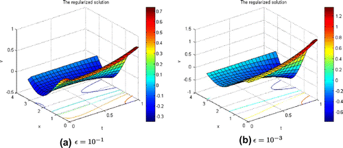
Figure 1. The regularized solution (49(49) $$\begin{array}{cc}\hfill v^{\mathit{ϵ}}\left(x,,,t\right)& =\sum _{1\le p\le N}\mathrm{\Phi }\left(\mathit{ϵ},,,p,,,t\right){\mathcal{M}}_p\left({\mathit{\phi }}^{\mathit{ϵ}},,,g^{\mathit{ϵ}}\right)cos\left(\left(p,-,\frac{1}{2}\right),x\right)\hfill \\ \hfill & +\sum _{1\le p\le N}\left({\int }_0^t,{\int }_0^{\mathit{\pi }},\mathrm{\Psi },\left(\mathit{ϵ},,,p,,,s,,,t\right),v^{\mathit{ϵ}},\left(x,,,s\right),cos,\left(\left(p,-,\frac{1}{2}\right),x\right),d,x,d,s\right)\hfill \\ \hfill & \times cos\left(\left(p,-,\frac{1}{2}\right),x\right)\hfill \\ \hfill & +\frac{1}{2}\sum _{1\le p\le N}{e}^{-\left(p,-,\frac{1}{2}\right)t}{\mathcal{M}}_p\left({\mathit{\phi }}^{\mathit{ϵ}},,,-,g^{\mathit{ϵ}}\right)cos\left(\left(p,-,\frac{1}{2}\right),x\right)\hfill \\ \hfill & -\sum _{1\le p\le N}\left(\frac{2}{\mathit{\pi }\left(2,p,-,1\right)},{\int }_0^t,{\int }_0^{\mathit{\pi }},e^{\left(p,-,\frac{1}{2}\right)\left(s,-,t\right)},v^{\mathit{ϵ}},\left(x,,,s\right),cos,\left(\left(p,-,\frac{1}{2}\right),x\right),d,x,d,s\right)\hfill \\ \hfill & \times cos\left(\left(p,-,\frac{1}{2}\right),x\right),\hfill \end{array}$$(49) ) of Example 1 for $h\left(x\right)=x^2\left(\mathit{\pi },-,x\right)$ and $\mathit{ϵ}={10}^{-r}$ with $r=2;4$ in 3-D representation.

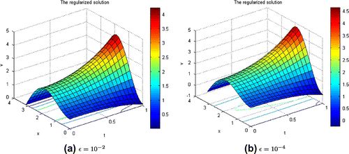
Figure 2. The exact solution (47(47) $$\begin{array}{cc}& u\left(x,,,t\right)\hfill \\ \hfill & =\frac{2}{\mathit{\pi }}\sum _{1\le p\le N}\frac{cosh\left(t,\sqrt{{\left(p,-,\frac{1}{2}\right)}^2+1}\right)}{cosh\left(\sqrt{{\left(p,-,\frac{1}{2}\right)}^2+1}\right)}〈h,\left(\mathit{\xi }\right),,,cos,\left(\left(p,-,\frac{1}{2}\right),\mathit{\xi }\right)〉cos\left(\left(p,-,\frac{1}{2}\right),x\right).\hfill \end{array}$$(47) ) for both two test functions in 3-D representation in Example 1.

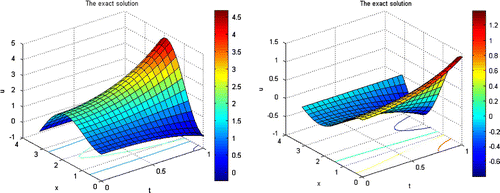
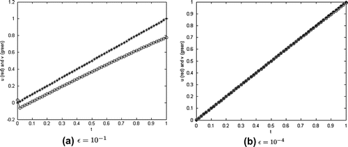
Figure 3. 2-D graphs of the exact solution (red) and regularized solution (green) at $x={\displaystyle \frac{\mathit{\pi }}{2}}$ for $h\left(x\right)=x^2\left(\mathit{\pi },-,x\right)$ and $\mathit{ϵ}={10}^{-r}$ with $r=2;4$ in Example 1.

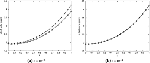
Figure 4. The regularized solution (49(49) $$\begin{array}{cc}\hfill v^{\mathit{ϵ}}\left(x,,,t\right)& =\sum _{1\le p\le N}\mathrm{\Phi }\left(\mathit{ϵ},,,p,,,t\right){\mathcal{M}}_p\left({\mathit{\phi }}^{\mathit{ϵ}},,,g^{\mathit{ϵ}}\right)cos\left(\left(p,-,\frac{1}{2}\right),x\right)\hfill \\ \hfill & +\sum _{1\le p\le N}\left({\int }_0^t,{\int }_0^{\mathit{\pi }},\mathrm{\Psi },\left(\mathit{ϵ},,,p,,,s,,,t\right),v^{\mathit{ϵ}},\left(x,,,s\right),cos,\left(\left(p,-,\frac{1}{2}\right),x\right),d,x,d,s\right)\hfill \\ \hfill & \times cos\left(\left(p,-,\frac{1}{2}\right),x\right)\hfill \\ \hfill & +\frac{1}{2}\sum _{1\le p\le N}{e}^{-\left(p,-,\frac{1}{2}\right)t}{\mathcal{M}}_p\left({\mathit{\phi }}^{\mathit{ϵ}},,,-,g^{\mathit{ϵ}}\right)cos\left(\left(p,-,\frac{1}{2}\right),x\right)\hfill \\ \hfill & -\sum _{1\le p\le N}\left(\frac{2}{\mathit{\pi }\left(2,p,-,1\right)},{\int }_0^t,{\int }_0^{\mathit{\pi }},e^{\left(p,-,\frac{1}{2}\right)\left(s,-,t\right)},v^{\mathit{ϵ}},\left(x,,,s\right),cos,\left(\left(p,-,\frac{1}{2}\right),x\right),d,x,d,s\right)\hfill \\ \hfill & \times cos\left(\left(p,-,\frac{1}{2}\right),x\right),\hfill \end{array}$$(49) ) of Example 1 for $h\left(x\right)={\sum }_{k=1}^3\frac{cos\left(k,x\right)}{k}$ and $\mathit{ϵ}={10}^{-r}$ with $r=1;3$ in 3-D representation.

Figure 5. 2-D graphs of the exact solution (red) and regularized solution (green) at $x={\displaystyle \frac{\mathit{\pi }}{2}}$ for $h\left(x\right)={\sum }_{k=1}^3\frac{cos\left(k,x\right)}{k}$ and $\mathit{ϵ}={10}^{-r}$ with $r=1;3;5;7$ in Example 1.

4.2. Comments

In these computations, the square grid size for time and space variables are set by choosing $K_1=M=20$. The truncation term is simply equal to $N=3$. (Figure 1).

Tables 1 and 2 show the absolute error at the midpoint ${\displaystyle \frac{\mathit{\pi }}{2}}$ and RRMS error defined in (43(43) $$\begin{array}{cc}& E\left(t_i\right)=\left|u,\left(\frac{\mathit{\pi }}{2},,,t_i\right),-,v^{\mathit{ϵ}},\left(\frac{\mathit{\pi }}{2},,,t_i\right)\right|,\hfill \end{array}$$(43) ) and (44(44) $$\begin{array}{cc}& RRMS\left(t_i\right)=\frac{\sqrt{\sum _{0\le j\le K}{\left|u,\left(x_j,,,t_i\right),-,v^{\mathit{ϵ}},\left(x_j,,,t_i\right)\right|}^2}}{\sqrt{\sum _{0\le j\le K}{\left|u,\left(x_j,,,t_i\right)\right|}^2}}.\hfill \end{array}$$(44) ) for both two test functions $h$. Particularly, the tables show the errors between the exact solution whose existence is ensured under the test function $h$, recall that in this example we let $h\left(x\right)=x^2\left(\mathit{\pi },-,x\right)$ and $h\left(x\right)={\displaystyle {\sum }_{k=1}^3\frac{cos\left(k,x\right)}{k}}$, and the regularized solution (49(49) $$\begin{array}{cc}\hfill v^{\mathit{ϵ}}\left(x,,,t\right)& =\sum _{1\le p\le N}\mathrm{\Phi }\left(\mathit{ϵ},,,p,,,t\right){\mathcal{M}}_p\left({\mathit{\phi }}^{\mathit{ϵ}},,,g^{\mathit{ϵ}}\right)cos\left(\left(p,-,\frac{1}{2}\right),x\right)\hfill \\ \hfill & +\sum _{1\le p\le N}\left({\int }_0^t,{\int }_0^{\mathit{\pi }},\mathrm{\Psi },\left(\mathit{ϵ},,,p,,,s,,,t\right),v^{\mathit{ϵ}},\left(x,,,s\right),cos,\left(\left(p,-,\frac{1}{2}\right),x\right),d,x,d,s\right)\hfill \\ \hfill & \times cos\left(\left(p,-,\frac{1}{2}\right),x\right)\hfill \\ \hfill & +\frac{1}{2}\sum _{1\le p\le N}{e}^{-\left(p,-,\frac{1}{2}\right)t}{\mathcal{M}}_p\left({\mathit{\phi }}^{\mathit{ϵ}},,,-,g^{\mathit{ϵ}}\right)cos\left(\left(p,-,\frac{1}{2}\right),x\right)\hfill \\ \hfill & -\sum _{1\le p\le N}\left(\frac{2}{\mathit{\pi }\left(2,p,-,1\right)},{\int }_0^t,{\int }_0^{\mathit{\pi }},e^{\left(p,-,\frac{1}{2}\right)\left(s,-,t\right)},v^{\mathit{ϵ}},\left(x,,,s\right),cos,\left(\left(p,-,\frac{1}{2}\right),x\right),d,x,d,s\right)\hfill \\ \hfill & \times cos\left(\left(p,-,\frac{1}{2}\right),x\right),\hfill \end{array}$$(49) ) at the fixed time $t={\displaystyle \frac{1}{10}};{\displaystyle \frac{1}{2}};1$ indicating three basic stages of time, nearly initial–middle–final, are both considered. We observe that the further initial point, the slower the convergence speed and the smaller $\mathit{ϵ}$, the smaller are the errors.

For the test function $h\left(x\right)=x^2\left(\mathit{\pi },-,x\right)$, we show the corresponding exact solution in Figure 3 (left). Despite the same 3-D shape, it should be given attention to the colour bar of the regularized ones, especially the maximum values attaining on the bar. In addition, Figure 4 presents the 2-D graphs of the solutions at $x={\displaystyle \frac{\mathit{\pi }}{2}}$ for $\mathit{ϵ}={10}^{-2};{10}^{-4}$. By observation, the regularized solution is close to the exact one when $\mathit{ϵ}$ gets smaller.

Similarly, for the test function $h\left(x\right)={\displaystyle {\sum }_{k=1}^3\frac{cos\left(k,x\right)}{k}}$, we show in Figure 3 (right) the exact solution and in Figure 2 the regularized solution (49(49) $$\begin{array}{cc}\hfill v^{\mathit{ϵ}}\left(x,,,t\right)& =\sum _{1\le p\le N}\mathrm{\Phi }\left(\mathit{ϵ},,,p,,,t\right){\mathcal{M}}_p\left({\mathit{\phi }}^{\mathit{ϵ}},,,g^{\mathit{ϵ}}\right)cos\left(\left(p,-,\frac{1}{2}\right),x\right)\hfill \\ \hfill & +\sum _{1\le p\le N}\left({\int }_0^t,{\int }_0^{\mathit{\pi }},\mathrm{\Psi },\left(\mathit{ϵ},,,p,,,s,,,t\right),v^{\mathit{ϵ}},\left(x,,,s\right),cos,\left(\left(p,-,\frac{1}{2}\right),x\right),d,x,d,s\right)\hfill \\ \hfill & \times cos\left(\left(p,-,\frac{1}{2}\right),x\right)\hfill \\ \hfill & +\frac{1}{2}\sum _{1\le p\le N}{e}^{-\left(p,-,\frac{1}{2}\right)t}{\mathcal{M}}_p\left({\mathit{\phi }}^{\mathit{ϵ}},,,-,g^{\mathit{ϵ}}\right)cos\left(\left(p,-,\frac{1}{2}\right),x\right)\hfill \\ \hfill & -\sum _{1\le p\le N}\left(\frac{2}{\mathit{\pi }\left(2,p,-,1\right)},{\int }_0^t,{\int }_0^{\mathit{\pi }},e^{\left(p,-,\frac{1}{2}\right)\left(s,-,t\right)},v^{\mathit{ϵ}},\left(x,,,s\right),cos,\left(\left(p,-,\frac{1}{2}\right),x\right),d,x,d,s\right)\hfill \\ \hfill & \times cos\left(\left(p,-,\frac{1}{2}\right),x\right),\hfill \end{array}$$(49) ) for $\mathit{ϵ}={10}^{-1};{10}^{-3}$. In Figure 5, we present the 2-D graphs of the solutions at the middle point of space for $\mathit{ϵ}={10}^{-r}$ with $r=1;3;5;7$, respectively.

4.3. Example 2

In this example, we consider the Cauchy problem for an elliptic sine-Gordon equation:(57) $$\begin{array}{c}\hfill \left\{\begin{array}{cc}\frac{{\mathit{\partial }}^2}{\mathit{\partial }{t}^2}u\left(x,,,t\right)+\frac{{\mathit{\partial }}^2}{\mathit{\partial }{x}^2}u\left(x,,,t\right)=sin\left(u,\left(x,,,t\right)\right)-sin\left(t,sin,x\right)-tsinx,\hfill & \left(x,,,t\right)\in \left(0,,,\mathit{\pi }\right)\times \left(0,,,1\right),\hfill \\ u\left(0,,,t\right)=u\left(\mathit{\pi },,,t\right)=0,\hfill & t\in \left(0,,,1\right),\hfill \\ u\left(x,,,0\right)=0,\frac{\mathit{\partial }}{\mathit{\partial }t}u\left(x,,,0\right)=sinx,\hfill & x\in \left(0,,,\mathit{\pi }\right).\hfill \end{array}\right.\end{array}$$(57)

It is easy to see that for $\mathcal{D}\left(\mathcal{A}\right)=H_0^1\left(0,,,\mathit{\pi }\right)$, we have an orthonormal eigenbasis ${\mathit{\varphi }}_p\left(x\right)=\sqrt{{\displaystyle \frac{2}{\mathit{\pi }}}}sin\left(\sqrt{{\mathit{\lambda }}_p},x\right)$ in $L^2\left(0,,,\mathit{\pi }\right)$ and ${\mathit{\lambda }}_p=p^2$ is the corresponding eigenvalue. The exact solution is $u\left(x,,,t\right)=tsinx$. Based on (33(33) $$\begin{array}{cc}\hfill v^{\mathit{ϵ}}\left(t\right)& =\sum _{p\ge 1}\left[\mathrm{\Phi },\left(\mathit{\beta },,,{\mathit{\lambda }}_p,,,t\right),{\mathcal{M}}_p,\left({\mathit{\phi }}^{\mathit{ϵ}},,,g^{\mathit{ϵ}}\right),+,{\int }_0^t,\mathrm{\Psi },\left(\mathit{\beta },,,{\mathit{\lambda }}_p,,,s,,,t\right),〈f,\left(s,,,v^{\mathit{ϵ}},\left(s\right)\right),,,{\mathit{\varphi }}_p〉,d,s\right]{\mathit{\varphi }}_p\hfill \\ \hfill & +\sum _{p\ge 1}\left[\frac{e^{-\sqrt{{\mathit{\lambda }}_p}t}}{2},{\mathcal{M}}_p,\left({\mathit{\phi }}^{\mathit{ϵ}},,,-,g^{\mathit{ϵ}}\right),-,{\int }_0^t,\frac{e^{\sqrt{{\mathit{\lambda }}_p}\left(s,-,t\right)}}{2\sqrt{{\mathit{\lambda }}_p}},〈f,\left(s,,,v^{\mathit{ϵ}},\left(s\right)\right),,,{\mathit{\varphi }}_p〉,d,s\right]{\mathit{\varphi }}_p,\hfill \end{array}$$(33) ), we obtain the regularized solution:(58) $$\begin{array}{cc}\hfill v^{\mathit{ϵ}}\left(x,,,t\right)& =\sum _{1\le p\le N}\mathrm{\Phi }\left(\mathit{ϵ},,,p,,,t\right){\mathcal{M}}_p\left({\mathit{\phi }}^{\mathit{ϵ}},,,g^{\mathit{ϵ}}\right)sin\left(p,x\right)\hfill \\ \hfill & +\sum _{1\le p\le N}\left({\int }_0^t,{\int }_0^{\mathit{\pi }},\mathrm{\Psi },\left(\mathit{ϵ},,,p,,,s,,,t\right),sin,\left(v^{\mathit{ϵ}},\left(y,,,s\right)\right),sin,\left(p,y\right),d,y,d,s\right)sin\left(p,x\right)\hfill \\ \hfill & +\frac{1}{2}\sum _{1\le p\le N}{e}^{-pt}{\mathcal{M}}_p\left({\mathit{\phi }}^{\mathit{ϵ}},,,-,g^{\mathit{ϵ}}\right)sin\left(p,x\right)\hfill \\ \hfill & +\sum _{1\le p\le N}\left(\frac{1}{\mathit{\pi }p},{\int }_0^t,{\int }_0^{\mathit{\pi }},e^{p\left(s,-,t\right)},sin,\left(v^{\mathit{ϵ}},\left(y,,,s\right)\right),sin,\left(p,y\right),d,y,d,s\right)sin\left(p,x\right),\hfill \end{array}$$(58) where(59) $$\begin{array}{cc}& \mathrm{\Phi }\left(\mathit{ϵ},,,p,,,t\right)=\frac{e^{-p\left(1,-,t\right)}}{2p{\mathit{ϵ}}^{0.99}+2e^{-p}},\mathrm{\Psi }\left(\mathit{ϵ},,,p,,,s,,,t\right)=\frac{1}{\mathit{\pi }}\frac{e^{-p\left(1,+,s,-,t\right)}}{p^2{\mathit{ϵ}}^{0.99}+p{e}^{-p}},\hfill \end{array}$$(59) (60) $$\begin{array}{cc}& {\mathcal{M}}_p\left({\mathit{\phi }}^{\mathit{ϵ}},,,\pm ,g^{\mathit{ϵ}}\right)=\frac{2}{\mathit{\pi }}{\int }_0^{\mathit{\pi }}\left[{\mathit{\phi }}^{\mathit{ϵ}},\left(x\right),\pm ,\frac{g^{\mathit{ϵ}}\left(x\right)}{p}\right]sin\left(p,x\right)dx.\hfill \end{array}$$(60)

We compute $v_i^{\mathit{ϵ}}\left(x\right),i=\overline{1,M}$ from $v_0^{\mathit{ϵ}}\left(x\right)={\mathit{\phi }}^{\mathit{ϵ}}\left(x\right)$ from the following iterative scheme:(61) $$\begin{array}{c}\hfill v_i^{\mathit{ϵ}}\left(x\right)=\sum _{1\le p\le N}\left[\mathcal{R},\left(\mathit{ϵ},,,p,,,t_i\right),-,\mathcal{W},\left(\mathit{ϵ},,,p,,,t_i\right)\right]sin\left(p,x\right),\end{array}$$(61)

where(62) $$\begin{array}{cc}\hfill \mathcal{R}\left(\mathit{ϵ},,,p,,,t_i\right)& =\mathrm{\Phi }\left(\mathit{ϵ},,,p,,,t_i\right){\mathcal{M}}_p\left({\mathit{\phi }}^{\mathit{ϵ}},,,g^{\mathit{ϵ}}\right)+\frac{1}{2}{e}^{-p{t}_i}{\mathcal{M}}_p\left({\mathit{\phi }}^{\mathit{ϵ}},,,-,g^{\mathit{ϵ}}\right)\hfill \\ \hfill & +\sum _{1\le j\le i}{\int }_{t_{j-1}}^{t_j}{\int }_0^{\mathit{\pi }}\mathrm{\Psi }\left(\mathit{ϵ},,,p,,,s,,,t_i\right)\left[sin,\left(v_{j-1}^{\mathit{ϵ}},\left(x\right)\right)\right.\hfill \\ \hfill & \left.-,sin,\left(s,sin,x\right),-,s,sin,x\right]sin\left(p,x\right)dxds,\hfill \end{array}$$(62) (63) $$\begin{array}{cc}& \mathcal{W}\left(\mathit{ϵ},,,p,,,t_i\right)\hfill \\ \hfill & =\frac{1}{\mathit{\pi }p}\sum _{1\le j\le i}{\int }_{t_{j-1}}^{t_j}{\int }_0^{\mathit{\pi }}{e}^{p\left(s,-,t_i\right)}\left[sin,\left(v_{j-1}^{\mathit{ϵ}},\left(x\right)\right),-,sin,\left(s,sin,x\right),-,s,sin,x\right]sin\left(p,x\right)dxds.\hfill \end{array}$$(63)

We first split $\mathcal{R}\left(\mathit{ϵ},,,p,,,t_i\right)$ into three appropriate terms, a term ${\mathcal{R}}_1\left(\mathit{ϵ},,,p,,,t_i\right)$ including $\mathrm{\Phi }\left(\mathit{ϵ},,,p,,,t_i\right){\mathcal{M}}_p\left({\mathit{\phi }}^{\mathit{ϵ}},,,g^{\mathit{ϵ}}\right)+{\displaystyle \frac{1}{2}}{e}^{-p{t}_i}{\mathcal{M}}_p\left({\mathit{\phi }}^{\mathit{ϵ}},,,-,g^{\mathit{ϵ}}\right)$, a term ${\mathcal{R}}_2\left(\mathit{ϵ},,,p,,,t_i\right)$ including the nonlinearity $sin\left(v_{j-1}^{\mathit{ϵ}},\left(x\right)\right)$ and a term ${\mathcal{R}}_3\left(\mathit{ϵ},,,p,,,t_i\right)$ containing the rest of this sum. In order to compute ${\mathcal{R}}_2\left(\mathit{ϵ},,,p,,,t_i\right)$ and ${\mathcal{R}}_3\left(\mathit{ϵ},,,p,,,t_i\right)$, we apply Gauss-Legendre quadrature method (see [19]). In particular, we have(64) $$\begin{array}{cc}& {\int }_{t_{j-1}}^{t_j}{\int }_0^{\mathit{\pi }}\mathrm{\Psi }\left(\mathit{ϵ},,,p,,,s,,,t_i\right)sin\left(v_{j-1}^{\mathit{ϵ}},\left(x\right)\right)sin\left(p,x\right)dxds\hfill \\ \hfill & =\frac{1}{\mathit{\pi }}\frac{e^{-p\left(1,+,t_j,-,t_i\right)}-e^{-p\left(1,+,t_{j-1},-,t_i\right)}}{p^2{\mathit{ϵ}}^{0.99}+p{e}^{-p}}\hfill \\ \hfill & \times \sum _{r=0}^{r_0}{\mathit{\gamma }}_{r}sin\left(v_{j-1}^{\mathit{ϵ}},\left(x_r\right)\right)sin\left(p,x_r\right),\hfill \end{array}$$(64) (65) $$\begin{array}{cc}& {\int }_{t_{j-1}}^{t_j}{\int }_0^{\mathit{\pi }}\mathrm{\Psi }\left(\mathit{ϵ},,,p,,,s,,,t_i\right)\left[sin,\left(s,sin,x\right),+,s,sin,x\right]sin\left(p,x\right)dxds\hfill \\ \hfill & =\sum _{l=0}^{l_0}\sum _{r=0}^{r_0}{\mathit{\alpha }}_l{\mathit{\gamma }}_r\mathrm{\Psi }\left(\mathit{ϵ},,,p,,,t_l,,,t_i\right)\hfill \\ \hfill & \times \left[sin,\left(t_l,sin,x_r\right),+,t_l,sin,x_r\right]sin\left(p,x_r\right),\hfill \end{array}$$(65)

where $x_r$ and $t_l$ are abscissae in $\left[0,,,\mathit{\pi }\right]$ and $\left[t_{j-1},,,t_j\right]$, respectively, and ${\mathit{\alpha }}_l,{\mathit{\gamma }}_r$ are associated weights.

We also do the same way in computing (63(63) $$\begin{array}{cc}& \mathcal{W}\left(\mathit{ϵ},,,p,,,t_i\right)\hfill \\ \hfill & =\frac{1}{\mathit{\pi }p}\sum _{1\le j\le i}{\int }_{t_{j-1}}^{t_j}{\int }_0^{\mathit{\pi }}{e}^{p\left(s,-,t_i\right)}\left[sin,\left(v_{j-1}^{\mathit{ϵ}},\left(x\right)\right),-,sin,\left(s,sin,x\right),-,s,sin,x\right]sin\left(p,x\right)dxds.\hfill \end{array}$$(63) ). Hence, (61(61) $$\begin{array}{c}\hfill v_i^{\mathit{ϵ}}\left(x\right)=\sum _{1\le p\le N}\left[\mathcal{R},\left(\mathit{ϵ},,,p,,,t_i\right),-,\mathcal{W},\left(\mathit{ϵ},,,p,,,t_i\right)\right]sin\left(p,x\right),\end{array}$$(61) ) can be determined.

Table 3. The absolute error (43(43) $$\begin{array}{cc}& E\left(t_i\right)=\left|u,\left(\frac{\mathit{\pi }}{2},,,t_i\right),-,v^{\mathit{ϵ}},\left(\frac{\mathit{\pi }}{2},,,t_i\right)\right|,\hfill \end{array}$$(43) ) and RRMS error (44(44) $$\begin{array}{cc}& RRMS\left(t_i\right)=\frac{\sqrt{\sum _{0\le j\le K}{\left|u,\left(x_j,,,t_i\right),-,v^{\mathit{ϵ}},\left(x_j,,,t_i\right)\right|}^2}}{\sqrt{\sum _{0\le j\le K}{\left|u,\left(x_j,,,t_i\right)\right|}^2}}.\hfill \end{array}$$(44) ) for $t={\displaystyle \frac{1}{10}};{\displaystyle \frac{1}{2}};1$ in Example 2.

$\mathit{ϵ}$	$E\left({\displaystyle \frac{1}{10}}\right)$	$E\left({\displaystyle \frac{1}{2}}\right)$	$E\left(1\right)$
${10}^{-1}$	0.08645837	0.13156858	0.22165771
${10}^{-2}$	0.00569716	0.01518309	0.05640565
${10}^{-3}$	0.00106781	0.00278605	0.01439988
${10}^{-4}$	0.00010483	0.00081799	0.00869168
${10}^{-5}$	0.00003575	0.00061786	0.00787221
${10}^{-6}$	0.00001986	0.00059505	0.00784513
${10}^{-7}$	0.00001760	0.00059255	0.00784453
${10}^{-8}$	0.00001749	0.00059233	0.00784383
$\mathit{ϵ}$	$RRMS\left({\displaystyle \frac{1}{10}}\right)$	$RRMS\left({\displaystyle \frac{1}{2}}\right)$	$RRMS\left(1\right)$
${10}^{-1}$	0.79907586	0.25047342	0.19837153
${10}^{-2}$	0.04141241	0.02148155	0.04475023
${10}^{-3}$	0.00839941	0.00481902	0.01021375
${10}^{-4}$	0.00085871	0.00239193	0.00616566
${10}^{-5}$	0.00062733	0.00235911	0.00564466
${10}^{-6}$	0.00047678	0.00231441	0.00561887
${10}^{-7}$	0.00045135	0.00230669	0.00561813
${10}^{-8}$	0.00045089	0.00230654	0.00561767

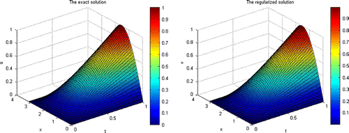
Figure 6. The exact solution $u\left(x,,,t\right)=tsinx$ (left) and the regularized solution $v^{\mathit{ϵ}}\left(x,,,t\right)$ (right) defined in (58(58) $$\begin{array}{cc}\hfill v^{\mathit{ϵ}}\left(x,,,t\right)& =\sum _{1\le p\le N}\mathrm{\Phi }\left(\mathit{ϵ},,,p,,,t\right){\mathcal{M}}_p\left({\mathit{\phi }}^{\mathit{ϵ}},,,g^{\mathit{ϵ}}\right)sin\left(p,x\right)\hfill \\ \hfill & +\sum _{1\le p\le N}\left({\int }_0^t,{\int }_0^{\mathit{\pi }},\mathrm{\Psi },\left(\mathit{ϵ},,,p,,,s,,,t\right),sin,\left(v^{\mathit{ϵ}},\left(y,,,s\right)\right),sin,\left(p,y\right),d,y,d,s\right)sin\left(p,x\right)\hfill \\ \hfill & +\frac{1}{2}\sum _{1\le p\le N}{e}^{-pt}{\mathcal{M}}_p\left({\mathit{\phi }}^{\mathit{ϵ}},,,-,g^{\mathit{ϵ}}\right)sin\left(p,x\right)\hfill \\ \hfill & +\sum _{1\le p\le N}\left(\frac{1}{\mathit{\pi }p},{\int }_0^t,{\int }_0^{\mathit{\pi }},e^{p\left(s,-,t\right)},sin,\left(v^{\mathit{ϵ}},\left(y,,,s\right)\right),sin,\left(p,y\right),d,y,d,s\right)sin\left(p,x\right),\hfill \end{array}$$(58) ) for $\mathit{ϵ}={10}^{-4}$ in 3-D representation in Example 2.

Figure 7. 2-D graphs of the exact solution (red) and regularized solution (green) for $\mathit{ϵ}={10}^{-r}$ with $r=1;4$ in Example 2.

4.4. Comments

In these computations, the finer grid is used $\left(K_1,=,M,=,60\right)$ and the truncation term $N$ is still fixed at $N=3$. As in Example 1, we show in Table 3 the errors between the exact solution $u\left(x,,,t\right)=tsinx$ and the regularized solution (58(58) $$\begin{array}{cc}\hfill v^{\mathit{ϵ}}\left(x,,,t\right)& =\sum _{1\le p\le N}\mathrm{\Phi }\left(\mathit{ϵ},,,p,,,t\right){\mathcal{M}}_p\left({\mathit{\phi }}^{\mathit{ϵ}},,,g^{\mathit{ϵ}}\right)sin\left(p,x\right)\hfill \\ \hfill & +\sum _{1\le p\le N}\left({\int }_0^t,{\int }_0^{\mathit{\pi }},\mathrm{\Psi },\left(\mathit{ϵ},,,p,,,s,,,t\right),sin,\left(v^{\mathit{ϵ}},\left(y,,,s\right)\right),sin,\left(p,y\right),d,y,d,s\right)sin\left(p,x\right)\hfill \\ \hfill & +\frac{1}{2}\sum _{1\le p\le N}{e}^{-pt}{\mathcal{M}}_p\left({\mathit{\phi }}^{\mathit{ϵ}},,,-,g^{\mathit{ϵ}}\right)sin\left(p,x\right)\hfill \\ \hfill & +\sum _{1\le p\le N}\left(\frac{1}{\mathit{\pi }p},{\int }_0^t,{\int }_0^{\mathit{\pi }},e^{p\left(s,-,t\right)},sin,\left(v^{\mathit{ϵ}},\left(y,,,s\right)\right),sin,\left(p,y\right),d,y,d,s\right)sin\left(p,x\right),\hfill \end{array}$$(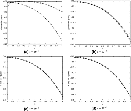58) ). In Figures 6 and 7, 3-D and 2-D graphs of them are shown, respectively. In particular, we show in Figure 7 the 2-D graphs describing how the regularized solution approaches the exact one when $\mathit{ϵ}$ becomes smaller and smaller for $\mathit{ϵ}={10}^{-1}$ to ${10}^{-4}$. We also show the 3-D representation of the regularized solution (with $\mathit{ϵ}={10}^{-4}$) in Figure 6 (right).

From the numerical results, we can conclude that the further the initial guess, the slower the convergence. On the other hand, it can be probably observed that the errors reduce slowly when $\mathit{ϵ}\to 0$ ($\mathit{ϵ}={10}^{-7},{10}^{-8},...$), and with a finer grid of resolution, we can have a better result in terms of smaller errors.

5. Conclusion

In this paper, we have studied a method to regularize the Cauchy problem for both linear and semi-linear elliptic equations which are severely ill-posed. Our approach is to present the solution of the problem in series representation, and then propose the regularized solution to control the strongly increasing coefficients appearing in the series. Under some prior assumptions, we deduce error estimates between the exact solution and regularized solution in Hilbert space norm. The convergence rate is established using logarithmic estimate. We apply fundamental tools, especially using contraction principle and Gronwall’s inequality, to prove these results (see more details in the Appendix 1).

In the numerical examples, we discussed semi-linear problems with the operator $\mathcal{A}=-\mathrm{\Delta }$ because of a wide range of applications. Thereby, we consider the linear modified Helmholtz equation and the elliptic nonlinear sine-Gordon equation. With lots of figures, tables and comments, our method is shown to be feasible and efficient. The code is written in MATLAB and the computations are done on a computer equipped with processor Pentium(R) Dual-Core CPU 2.30 GHz and having 3.0 GB total RAM.

The present paper gives some error estimates under a global Lipschitz case of source term $f$. This makes the applicability of the method quite narrow. In future, we will consider the regularized problem in the locally Lipschitz case of the source function $f$.

Acknowledgements

The authors would like to thank the anonymous referees for their valuable suggestions and comments leading to the improvement of our manuscript.

Notes

This work is supported by HCMC University of Science under grant T2014-1 and Vietnam National University Ho Chi Minh City (VNU-HCM) under [grant number B2014-18-01].

Appendix 1

In the appendix, we would like to present the proof of all theoretical results showed in Sections 2 and 3. On account of the proof of theorems intentionally divided into results of related lemmas, we will show the proofs of all lemmas first, then the results of theorems will become obvious to be concluded.

Proof of Lemma 1

From (16(16) $$\begin{array}{c}\hfill u^{\mathit{ϵ}}\left(t\right)=\sum _{p\ge 1}\left[{\displaystyle \frac{1}{2\mathit{\beta }+2e^{-\sqrt{{\mathit{\lambda }}_p}t}}},\left(〈\mathit{\phi },,,{\mathit{\varphi }}_p〉,+,\frac{〈g,,,{\mathit{\varphi }}_p〉}{\sqrt{{\mathit{\lambda }}_p}}\right),+,\frac{e^{-\sqrt{{\mathit{\lambda }}_p}t}}{2},\left(〈\mathit{\phi },,,{\mathit{\varphi }}_p〉,-,\frac{〈g,,,{\mathit{\varphi }}_p〉}{\sqrt{{\mathit{\lambda }}_p}}\right)\right]{\mathit{\varphi }}_p.\end{array}$$(16) ) to (17(17) $$\begin{array}{c}\hfill v^{\mathit{ϵ}}\left(t\right)=\sum _{p\ge 1}\left[,{\displaystyle \frac{1}{2\mathit{\beta }+2e^{-\sqrt{{\mathit{\lambda }}_p}t}}},\left(,〈{\mathit{\phi }}^{\mathit{ϵ}},,,{\mathit{\varphi }}_p〉,+,\frac{〈g^{\mathit{ϵ}},,,{\mathit{\varphi }}_p〉}{\sqrt{{\mathit{\lambda }}_p}},\right),+,\frac{e^{-\sqrt{{\mathit{\lambda }}_p}t}}{2},\left(,〈{\mathit{\phi }}^{\mathit{ϵ}},,,{\mathit{\varphi }}_p〉,-,\frac{〈g^{\mathit{ϵ}},,,{\mathit{\varphi }}_p〉}{\sqrt{{\mathit{\lambda }}_p}},\right),\right]{\mathit{\varphi }}_p.\end{array}$$(17) ), we have(A1) $$\begin{array}{cc}\hfill u^{\mathit{ϵ}}\left(t\right)-v^{\mathit{ϵ}}\left(t\right)& =\sum _{p\ge 1}\frac{1}{2\mathit{\beta }+2e^{-\sqrt{{\mathit{\lambda }}_p}t}}\left(〈\mathit{\phi },-,{\mathit{\phi }}^{\mathit{ϵ}},,,{\mathit{\varphi }}_p〉,+,\frac{〈g,-,g^{\mathit{ϵ}},,,{\mathit{\varphi }}_p〉}{\sqrt{{\mathit{\lambda }}_p}}\right){\mathit{\varphi }}_p\hfill \\ \hfill & +\sum _{p\ge 1}\frac{e^{-\sqrt{{\mathit{\lambda }}_p}t}}{2}\left(〈\mathit{\phi },-,{\mathit{\phi }}^{\mathit{ϵ}},,,{\mathit{\varphi }}_p〉,-,\frac{〈g,-,g^{\mathit{ϵ}},,,{\mathit{\varphi }}_p〉}{\sqrt{{\mathit{\lambda }}_p}}\right){\mathit{\varphi }}_p,\hfill \end{array}$$(A1)

By using the inequality ${\left(a,+,b,+,c,+,d\right)}^2\le 4\left(a^2,+,b^2,+,c^2,+,d^2\right)$, we get(A2) $$\begin{array}{cc}\hfill {\left|〈u^{\mathit{ϵ}},\left(t\right),-,v^{\mathit{ϵ}},\left(t\right),,,{\mathit{\varphi }}_p〉\right|}^2& \le \frac{1}{{\left(\mathit{\beta },+,e^{-\sqrt{{\mathit{\lambda }}_p}t}\right)}^2}\left({\left|〈\mathit{\phi },-,{\mathit{\phi }}^{\mathit{ϵ}},,,{\mathit{\varphi }}_p〉\right|}^2,+,\frac{{\left|〈g,-,g^{\mathit{ϵ}},,,{\mathit{\varphi }}_p〉\right|}^2}{{\mathit{\lambda }}_p}\right)\hfill \\ \hfill & +e^{-2\sqrt{{\mathit{\lambda }}_p}t}\left({\left|〈\mathit{\phi },-,{\mathit{\phi }}^{\mathit{ϵ}},,,{\mathit{\varphi }}_p〉\right|}^2,+,\frac{{\left|〈g,-,g^{\mathit{ϵ}},,,{\mathit{\varphi }}_p〉\right|}^2}{{\mathit{\lambda }}_p}\right).\hfill \end{array}$$(A2)

Since ${\mathit{\beta }}^2\le {\left(\mathit{\beta },+,e^{-\sqrt{{\mathit{\lambda }}_p}t}\right)}^2$ and $e^{-2\sqrt{{\mathit{\lambda }}_p}t}\le 1\le {\displaystyle \frac{1}{{\mathit{\beta }}^2}}$, it yields(A3) $$\begin{array}{cc}\hfill {∥u^{\mathit{ϵ}},\left(t\right),-,v^{\mathit{ϵ}},\left(t\right)∥}^2& =\sum _{p\ge 1}{\left|〈u^{\mathit{ϵ}},\left(t\right),-,v^{\mathit{ϵ}},\left(t\right),,,{\mathit{\varphi }}_p〉\right|}^2\le \frac{2}{{\mathit{\beta }}^2}\sum _{p\ge 1}\left({\left|〈\mathit{\phi },-,{\mathit{\phi }}^{\mathit{ϵ}},,,{\mathit{\varphi }}_p〉\right|}^2,+,\frac{{\left|〈g,-,g^{\mathit{ϵ}},,,{\mathit{\varphi }}_p〉\right|}^2}{{\mathit{\lambda }}_1}\right)\hfill \\ \hfill & \le \frac{2}{{\mathit{\beta }}^2}\left(∥\mathit{\phi },-,{\mathit{\phi }}^{\mathit{ϵ}}∥,+,\frac{∥g,-,g^{\mathit{ϵ}}∥}{{\mathit{\lambda }}_1}\right).\hfill \end{array}$$(A3)

Applying (3(3) $$\begin{array}{c}\hfill ∥\mathit{\phi },-,{\mathit{\phi }}^{\mathit{ϵ}}∥\le \mathit{ϵ},∥g,-,g^{\mathit{ϵ}}∥\le \mathit{ϵ},\end{array}$$(3) ) to this, we obtain the desired result. $\square$

Proof of Lemma 2

By taking the derivative of $u\left(t\right)$ in (8(8) $$\begin{array}{c}\hfill u(t)=\sum _{p=1}^{\infty }\left[cosh,\left(\sqrt{{\mathit{\lambda }}_p},t\right),〈\mathit{\phi },,,{\mathit{\varphi }}_p〉,+,\frac{sinh\left(\sqrt{{\mathit{\lambda }}_p},t\right)}{\sqrt{{\mathit{\lambda }}_p}},〈g,,,{\mathit{\varphi }}_p〉\right]{\mathit{\varphi }}_p.\end{array}$$(8) ) with respect to $t$, we obtain(A4) $$\begin{array}{c}\hfill \frac{\mathit{\partial }}{\mathit{\partial }t}u\left(t\right)=\sum _{p\ge 1}\sqrt{{\mathit{\lambda }}_p}\frac{e^{\sqrt{{\mathit{\lambda }}_p}t}}{2}\left(〈\mathit{\phi },,,{\mathit{\varphi }}_p〉,+,\frac{〈g,,,{\mathit{\varphi }}_p〉}{\sqrt{{\mathit{\lambda }}_p}}\right){\mathit{\varphi }}_p-\sum _{p\ge 1}\sqrt{{\mathit{\lambda }}_p}\frac{e^{-\sqrt{{\mathit{\lambda }}_p}t}}{2}\left(〈\mathit{\phi },,,{\mathit{\varphi }}_p〉,+,\frac{〈g,,,{\mathit{\varphi }}_p〉}{\sqrt{{\mathit{\lambda }}_p}}\right){\mathit{\varphi }}_p.\end{array}$$(A4)

It follows from (8(8) $$\begin{array}{c}\hfill u(t)=\sum _{p=1}^{\infty }\left[cosh,\left(\sqrt{{\mathit{\lambda }}_p},t\right),〈\mathit{\phi },,,{\mathit{\varphi }}_p〉,+,\frac{sinh\left(\sqrt{{\mathit{\lambda }}_p},t\right)}{\sqrt{{\mathit{\lambda }}_p}},〈g,,,{\mathit{\varphi }}_p〉\right]{\mathit{\varphi }}_p.\end{array}$$(8) ) and (A4(A4) $$\begin{array}{c}\hfill \frac{\mathit{\partial }}{\mathit{\partial }t}u\left(t\right)=\sum _{p\ge 1}\sqrt{{\mathit{\lambda }}_p}\frac{e^{\sqrt{{\mathit{\lambda }}_p}t}}{2}\left(〈\mathit{\phi },,,{\mathit{\varphi }}_p〉,+,\frac{〈g,,,{\mathit{\varphi }}_p〉}{\sqrt{{\mathit{\lambda }}_p}}\right){\mathit{\varphi }}_p-\sum _{p\ge 1}\sqrt{{\mathit{\lambda }}_p}\frac{e^{-\sqrt{{\mathit{\lambda }}_p}t}}{2}\left(〈\mathit{\phi },,,{\mathit{\varphi }}_p〉,+,\frac{〈g,,,{\mathit{\varphi }}_p〉}{\sqrt{{\mathit{\lambda }}_p}}\right){\mathit{\varphi }}_p.\end{array}$$(A4) ) that(A5) $$\begin{array}{c}\hfill 〈\mathit{\phi },,,{\mathit{\varphi }}_p〉+\frac{〈g,,,{\mathit{\varphi }}_p〉}{\sqrt{{\mathit{\lambda }}_p}}=e^{-\sqrt{{\mathit{\lambda }}_p}t}\left(〈u,\left(t\right),,,{\mathit{\varphi }}_p〉,+,\frac{〈\frac{\mathit{\partial }}{\mathit{\partial }t},u,\left(t\right),,,{\mathit{\varphi }}_p〉}{\sqrt{{\mathit{\lambda }}_p}}\right).\end{array}$$(A5)

We subtract $u^{\mathit{ϵ}}\left(t\right)$ from $u\left(t\right)$ to obtain(A6) $$\begin{array}{cc}\hfill u\left(t\right)-u^{\mathit{ϵ}}\left(t\right)& =\sum _{p\ge 1}\left(\frac{e^{\sqrt{{\mathit{\lambda }}_p}t}}{2},-,\frac{1}{2\mathit{\beta }+2e^{-\sqrt{{\mathit{\lambda }}_p}t}}\right)\left(〈\mathit{\phi },,,{\mathit{\varphi }}_p〉,+,\frac{〈g,,,{\mathit{\varphi }}_p〉}{\sqrt{{\mathit{\lambda }}_p}}\right){\mathit{\varphi }}_p\hfill \\ \hfill & =\sum _{p\ge 1}\frac{\mathit{\beta }{e}^{\sqrt{{\mathit{\lambda }}_p}\left(t,-,T\right)}}{2\mathit{\beta }+2e^{-\sqrt{{\mathit{\lambda }}_p}t}}\left(〈u,\left(T\right),,,{\mathit{\varphi }}_p〉,+,\frac{〈\frac{\mathit{\partial }}{\mathit{\partial }t},u,\left(T\right),,,{\mathit{\varphi }}_p〉}{\sqrt{{\mathit{\lambda }}_p}}\right){\mathit{\varphi }}_p.\hfill \end{array}$$(A6)

Finally, we obtain(A7) $$\begin{array}{c}\hfill {∥u,\left(t\right),-,u^{\mathit{ϵ}},\left(t\right)∥}^2=\sum _{p\ge 1}{\left(\frac{\mathit{\beta }{e}^{\sqrt{{\mathit{\lambda }}_p}\left(t,-,T\right)}}{2\mathit{\beta }+2e^{-\sqrt{{\mathit{\lambda }}_p}t}}\right)}^2{\left(〈u,\left(T\right),,,{\mathit{\varphi }}_p〉,+,\frac{〈\frac{\mathit{\partial }}{\mathit{\partial }t},u,\left(T\right),,,{\mathit{\varphi }}_p〉}{\sqrt{{\mathit{\lambda }}_p}}\right)}^2.\end{array}$$(A7)

In the next step, to get the result, we have two cases.

(1)

For $t\in \left[0,,,{\displaystyle \frac{T}{2}}\right]$, ${∥u,\left(t\right),-,u^{\mathit{ϵ}},\left(t\right)∥}^2$ in (A7(A7) $$\begin{array}{c}\hfill {∥u,\left(t\right),-,u^{\mathit{ϵ}},\left(t\right)∥}^2=\sum _{p\ge 1}{\left(\frac{\mathit{\beta }{e}^{\sqrt{{\mathit{\lambda }}_p}\left(t,-,T\right)}}{2\mathit{\beta }+2e^{-\sqrt{{\mathit{\lambda }}_p}t}}\right)}^2{\left(〈u,\left(T\right),,,{\mathit{\varphi }}_p〉,+,\frac{〈\frac{\mathit{\partial }}{\mathit{\partial }t},u,\left(T\right),,,{\mathit{\varphi }}_p〉}{\sqrt{{\mathit{\lambda }}_p}}\right)}^2.\end{array}$$(A7) ) can be estimated as(A8) $$\begin{array}{cc}\hfill {∥u,\left(t\right),-,u^{\mathit{ϵ}},\left(t\right)∥}^2& \le \frac{{\mathit{\beta }}^2}{4}\sum _{p\ge 1}{\left(〈u,\left(T\right),,,{\mathit{\varphi }}_p〉,+,\frac{〈\frac{\mathit{\partial }}{\mathit{\partial }t},u,\left(T\right),,,{\mathit{\varphi }}_p〉}{\sqrt{{\mathit{\lambda }}_p}}\right)}^2\hfill \\ \hfill & \le \frac{{\mathit{\beta }}^2}{2}\left({∥u,\left(T\right)∥}^2,+,\frac{{∥\frac{\mathit{\partial }}{\mathit{\partial }t},u,\left(T\right)∥}^2}{{\mathit{\lambda }}_1}\right),\hfill \end{array}$$(A8) since $e^{\sqrt{{\mathit{\lambda }}_p}\left(t,-,T\right)}\le e^{-\sqrt{{\mathit{\lambda }}_p}t}$. This implies the first estimate in (25(25) $$\begin{array}{c}\hfill \left\{\begin{array}{cc}∥u,\left(t\right),-,u^{\mathit{ϵ}},\left(t\right)∥\le \mathit{\beta }{E}_1,\hfill & t\in \left[0,,,\frac{T}{2}\right],\hfill \\ ∥u,\left(t\right),-,u^{\mathit{ϵ}},\left(t\right)∥\le {\mathit{\beta }}^{\frac{T-t}{t}}{E}_1,\hfill & t\in \left[\frac{T}{2},,,T\right].\hfill \end{array}\right.\end{array}$$(25) ) under condition (18(18) $$\begin{array}{c}\hfill \sqrt{\frac{{∥u,\left(T\right)∥}^2}{2}+\frac{{∥{\displaystyle \frac{\mathit{\partial }}{\mathit{\partial }t}},u,\left(T\right)∥}^2}{2{\mathit{\lambda }}_1}}<E_1,\end{array}$$(18) ).

(2)

For $t\in \left[{\displaystyle \frac{T}{2}},,,T\right]$, the second estimate in (25(25) $$\begin{array}{c}\hfill \left\{\begin{array}{cc}∥u,\left(t\right),-,u^{\mathit{ϵ}},\left(t\right)∥\le \mathit{\beta }{E}_1,\hfill & t\in \left[0,,,\frac{T}{2}\right],\hfill \\ ∥u,\left(t\right),-,u^{\mathit{ϵ}},\left(t\right)∥\le {\mathit{\beta }}^{\frac{T-t}{t}}{E}_1,\hfill & t\in \left[\frac{T}{2},,,T\right].\hfill \end{array}\right.\end{array}$$(25) ) is obtained similarly using the fact that ${\displaystyle \frac{e^{\sqrt{{\mathit{\lambda }}_p}\left(t,-,T\right)}}{\mathit{\beta }+e^{-\sqrt{{\mathit{\lambda }}_p}t}}}\le {\mathit{\beta }}^{\frac{T-t}{t}-1}$.

This completes the proof.$\square$

Proof of Lemma 3

We now rewrite the difference between $u\left(t\right)$ and $u^{\mathit{ϵ}}\left(t\right)$.(A9) $$\begin{array}{c}\hfill u\left(t\right)-u^{\mathit{ϵ}}\left(t\right)=\sum _{p\ge 1}\frac{\mathit{\beta }}{2\mathit{\beta }\sqrt{{\mathit{\lambda }}_p}+2\sqrt{{\mathit{\lambda }}_p}{e}^{-\sqrt{{\mathit{\lambda }}_p}t}}\left(\sqrt{{\mathit{\lambda }}_p},〈u,\left(t\right),,,{\mathit{\varphi }}_p〉,+,〈\frac{\mathit{\partial }}{\mathit{\partial }t},u,\left(t\right),,,{\mathit{\varphi }}_p〉\right){\mathit{\varphi }}_p.\end{array}$$(A9)

We note that $e^{-\sqrt{{\mathit{\lambda }}_p}T}\left(\sqrt{{\mathit{\lambda }}_p},〈u,\left(T\right),,,{\mathit{\varphi }}_p〉,+,〈\frac{\mathit{\partial }}{\mathit{\partial }t},u,\left(T\right),,,{\mathit{\varphi }}_p〉\right)=e^{-\sqrt{{\mathit{\lambda }}_p}t}(\sqrt{{\mathit{\lambda }}_p}〈u,\left(t\right),,,{\mathit{\varphi }}_p〉+〈\frac{\mathit{\partial }}{\mathit{\partial }t},u,\left(t\right),,,{\mathit{\varphi }}_p〉)$, then it follows(A10) $$\begin{array}{c}\hfill e^{\sqrt{{\mathit{\lambda }}_p}\left(T,-,t\right)}\left(\sqrt{{\mathit{\lambda }}_p},〈u,\left(t\right),,,{\mathit{\varphi }}_p〉,+,〈\frac{\mathit{\partial }}{\mathit{\partial }t},u,\left(t\right),,,{\mathit{\varphi }}_p〉\right)=\sqrt{{\mathit{\lambda }}_p}〈u,\left(T\right),,,{\mathit{\varphi }}_p〉+〈\frac{\mathit{\partial }}{\mathit{\partial }t},u,\left(T\right),,,{\mathit{\varphi }}_p〉.\end{array}$$(A10)

Thus, (A9(A9) $$\begin{array}{c}\hfill u\left(t\right)-u^{\mathit{ϵ}}\left(t\right)=\sum _{p\ge 1}\frac{\mathit{\beta }}{2\mathit{\beta }\sqrt{{\mathit{\lambda }}_p}+2\sqrt{{\mathit{\lambda }}_p}{e}^{-\sqrt{{\mathit{\lambda }}_p}t}}\left(\sqrt{{\mathit{\lambda }}_p},〈u,\left(t\right),,,{\mathit{\varphi }}_p〉,+,〈\frac{\mathit{\partial }}{\mathit{\partial }t},u,\left(t\right),,,{\mathit{\varphi }}_p〉\right){\mathit{\varphi }}_p.\end{array}$$(A9) ) becomes(A11) $$\begin{array}{c}\hfill u\left(t\right)-u^{\mathit{ϵ}}\left(t\right)=\sum _{p\ge 1}\frac{\mathit{\beta }{e}^{-\sqrt{{\mathit{\lambda }}_p}\left(T,-,t\right)}}{2\mathit{\beta }\sqrt{{\mathit{\lambda }}_p}+2\sqrt{{\mathit{\lambda }}_p}{e}^{-\sqrt{{\mathit{\lambda }}_p}t}}\left(\sqrt{{\mathit{\lambda }}_p},〈u,\left(T\right),,,{\mathit{\varphi }}_p〉,+,〈\frac{\mathit{\partial }}{\mathit{\partial }t},u,\left(T\right),,,{\mathit{\varphi }}_p〉\right){\mathit{\varphi }}_p.\end{array}$$(A11)

On the other hand, we have(A12) $$\begin{array}{c}\hfill \frac{\mathit{\beta }{e}^{-\sqrt{{\mathit{\lambda }}_p}\left(T,-,t\right)}}{2\mathit{\beta }\sqrt{{\mathit{\lambda }}_p}+2\sqrt{{\mathit{\lambda }}_p}{e}^{-\sqrt{{\mathit{\lambda }}_p}t}}\le \frac{\mathit{\beta }}{2\sqrt{{\mathit{\lambda }}_1}}\frac{e^{-\sqrt{{\mathit{\lambda }}_p}\left(T,-,t\right)}}{\frac{\mathit{\beta }}{\sqrt{{\mathit{\lambda }}_1}}\sqrt{{\mathit{\lambda }}_p}+e^{-\sqrt{{\mathit{\lambda }}_p}t}}.\end{array}$$(A12)

From (A11(A11) $$\begin{array}{c}\hfill u\left(t\right)-u^{\mathit{ϵ}}\left(t\right)=\sum _{p\ge 1}\frac{\mathit{\beta }{e}^{-\sqrt{{\mathit{\lambda }}_p}\left(T,-,t\right)}}{2\mathit{\beta }\sqrt{{\mathit{\lambda }}_p}+2\sqrt{{\mathit{\lambda }}_p}{e}^{-\sqrt{{\mathit{\lambda }}_p}t}}\left(\sqrt{{\mathit{\lambda }}_p},〈u,\left(T\right),,,{\mathit{\varphi }}_p〉,+,〈\frac{\mathit{\partial }}{\mathit{\partial }t},u,\left(T\right),,,{\mathit{\varphi }}_p〉\right){\mathit{\varphi }}_p.\end{array}$$(A11) ) to (A12(A12) $$\begin{array}{c}\hfill \frac{\mathit{\beta }{e}^{-\sqrt{{\mathit{\lambda }}_p}\left(T,-,t\right)}}{2\mathit{\beta }\sqrt{{\mathit{\lambda }}_p}+2\sqrt{{\mathit{\lambda }}_p}{e}^{-\sqrt{{\mathit{\lambda }}_p}t}}\le \frac{\mathit{\beta }}{2\sqrt{{\mathit{\lambda }}_1}}\frac{e^{-\sqrt{{\mathit{\lambda }}_p}\left(T,-,t\right)}}{\frac{\mathit{\beta }}{\sqrt{{\mathit{\lambda }}_1}}\sqrt{{\mathit{\lambda }}_p}+e^{-\sqrt{{\mathit{\lambda }}_p}t}}.\end{array}$$(A12) ), as in proof of Lemma 2, we will consider two cases.

(1)

For $t\in \left[0,,,{\displaystyle \frac{T}{2}}\right]$, we get(A13) $$\begin{array}{c}\hfill \frac{\mathit{\beta }{e}^{-\sqrt{{\mathit{\lambda }}_p}\left(T,-,t\right)}}{2\mathit{\beta }\sqrt{{\mathit{\lambda }}_p}+2\sqrt{{\mathit{\lambda }}_p}{e}^{-\sqrt{{\mathit{\lambda }}_p}t}}\le \frac{\mathit{\beta }}{2\sqrt{{\mathit{\lambda }}_1}}.\end{array}$$(A13) Consequently, we obtain from (A11(A11) $$\begin{array}{c}\hfill u\left(t\right)-u^{\mathit{ϵ}}\left(t\right)=\sum _{p\ge 1}\frac{\mathit{\beta }{e}^{-\sqrt{{\mathit{\lambda }}_p}\left(T,-,t\right)}}{2\mathit{\beta }\sqrt{{\mathit{\lambda }}_p}+2\sqrt{{\mathit{\lambda }}_p}{e}^{-\sqrt{{\mathit{\lambda }}_p}t}}\left(\sqrt{{\mathit{\lambda }}_p},〈u,\left(T\right),,,{\mathit{\varphi }}_p〉,+,〈\frac{\mathit{\partial }}{\mathit{\partial }t},u,\left(T\right),,,{\mathit{\varphi }}_p〉\right){\mathit{\varphi }}_p.\end{array}$$(A11) ) to (A13(A13) $$\begin{array}{c}\hfill \frac{\mathit{\beta }{e}^{-\sqrt{{\mathit{\lambda }}_p}\left(T,-,t\right)}}{2\mathit{\beta }\sqrt{{\mathit{\lambda }}_p}+2\sqrt{{\mathit{\lambda }}_p}{e}^{-\sqrt{{\mathit{\lambda }}_p}t}}\le \frac{\mathit{\beta }}{2\sqrt{{\mathit{\lambda }}_1}}.\end{array}$$(A13) ) that(A14) $$\begin{array}{c}\hfill {∥u,\left(t\right),-,u^{\mathit{ϵ}},\left(t\right)∥}^2\le \frac{{\mathit{\beta }}^2}{4{\mathit{\lambda }}_1}\sum _{p\ge 1}{\left(\sqrt{{\mathit{\lambda }}_p},〈u,\left(T\right),,,{\mathit{\varphi }}_p〉,+,〈\frac{\mathit{\partial }}{\mathit{\partial }t},u,\left(T\right),,,{\mathit{\varphi }}_p〉\right)}^2\le \frac{{\mathit{\beta }}^2}{4{\mathit{\lambda }}_1}{E}_2^2,\end{array}$$(A14) which implies the first estimate in (26(26) $$\begin{array}{c}\hfill \left\{\begin{array}{cc}∥u,\left(t\right),-,u^{\mathit{ϵ}},\left(t\right)∥\le \frac{\mathit{\beta }}{2\sqrt{{\mathit{\lambda }}_1}}{E}_2,\hfill & t\in \left[0,,,\frac{T}{2}\right],\hfill \\ ∥u,\left(t\right),-,u^{\mathit{ϵ}},\left(t\right)∥\le \frac{1}{2\sqrt{{\mathit{\lambda }}_1}}{\mathit{\beta }}^{\frac{T-t}{t}}{E}_2,\hfill & t\in \left[\frac{T}{2},,,T\right].\hfill \end{array}\right.\end{array}$$(26) ).

(2)

For $t\in \left[{\displaystyle \frac{T}{2}},,,T\right]$, it follows from (A12(A12) $$\begin{array}{c}\hfill \frac{\mathit{\beta }{e}^{-\sqrt{{\mathit{\lambda }}_p}\left(T,-,t\right)}}{2\mathit{\beta }\sqrt{{\mathit{\lambda }}_p}+2\sqrt{{\mathit{\lambda }}_p}{e}^{-\sqrt{{\mathit{\lambda }}_p}t}}\le \frac{\mathit{\beta }}{2\sqrt{{\mathit{\lambda }}_1}}\frac{e^{-\sqrt{{\mathit{\lambda }}_p}\left(T,-,t\right)}}{\frac{\mathit{\beta }}{\sqrt{{\mathit{\lambda }}_1}}\sqrt{{\mathit{\lambda }}_p}+e^{-\sqrt{{\mathit{\lambda }}_p}t}}.\end{array}$$(A12) ) that(A15) $$\begin{array}{cc}\hfill \frac{\mathit{\beta }{e}^{-\sqrt{{\mathit{\lambda }}_p}\left(T,-,t\right)}}{2\mathit{\beta }\sqrt{{\mathit{\lambda }}_p}+2\sqrt{{\mathit{\lambda }}_p}{e}^{-\sqrt{{\mathit{\lambda }}_p}t}}& \le \frac{\mathit{\beta }}{2\sqrt{{\mathit{\lambda }}_1}}{\left[\frac{T}{\frac{\mathit{\beta }}{\sqrt{{\mathit{\lambda }}_1}}\left(1,+,ln,\left(\frac{T}{\frac{\mathit{\beta }}{\sqrt{{\mathit{\lambda }}_1}}}\right)\right)}\right]}^{\frac{2t-T}{t}}\hfill \\ \hfill & \le \frac{1}{2\sqrt{{\mathit{\lambda }}_1}}{\mathit{\beta }}^{\frac{T-t}{t}}{\left[\frac{\sqrt{{\mathit{\lambda }}_1}T}{1+ln\left(\frac{\sqrt{{\mathit{\lambda }}_1}T}{\mathit{\beta }}\right)}\right]}^{\frac{2t-T}{t}}.\hfill \end{array}$$(A15) Then, combining (A11(A11) $$\begin{array}{c}\hfill u\left(t\right)-u^{\mathit{ϵ}}\left(t\right)=\sum _{p\ge 1}\frac{\mathit{\beta }{e}^{-\sqrt{{\mathit{\lambda }}_p}\left(T,-,t\right)}}{2\mathit{\beta }\sqrt{{\mathit{\lambda }}_p}+2\sqrt{{\mathit{\lambda }}_p}{e}^{-\sqrt{{\mathit{\lambda }}_p}t}}\left(\sqrt{{\mathit{\lambda }}_p},〈u,\left(T\right),,,{\mathit{\varphi }}_p〉,+,〈\frac{\mathit{\partial }}{\mathit{\partial }t},u,\left(T\right),,,{\mathit{\varphi }}_p〉\right){\mathit{\varphi }}_p.\end{array}$$(A11) )-(A15(A15) $$\begin{array}{cc}\hfill \frac{\mathit{\beta }{e}^{-\sqrt{{\mathit{\lambda }}_p}\left(T,-,t\right)}}{2\mathit{\beta }\sqrt{{\mathit{\lambda }}_p}+2\sqrt{{\mathit{\lambda }}_p}{e}^{-\sqrt{{\mathit{\lambda }}_p}t}}& \le \frac{\mathit{\beta }}{2\sqrt{{\mathit{\lambda }}_1}}{\left[\frac{T}{\frac{\mathit{\beta }}{\sqrt{{\mathit{\lambda }}_1}}\left(1,+,ln,\left(\frac{T}{\frac{\mathit{\beta }}{\sqrt{{\mathit{\lambda }}_1}}}\right)\right)}\right]}^{\frac{2t-T}{t}}\hfill \\ \hfill & \le \frac{1}{2\sqrt{{\mathit{\lambda }}_1}}{\mathit{\beta }}^{\frac{T-t}{t}}{\left[\frac{\sqrt{{\mathit{\lambda }}_1}T}{1+ln\left(\frac{\sqrt{{\mathit{\lambda }}_1}T}{\mathit{\beta }}\right)}\right]}^{\frac{2t-T}{t}}.\hfill \end{array}$$(A15) ) gives the second estimate in (26(26) $$\begin{array}{c}\hfill \left\{\begin{array}{cc}∥u,\left(t\right),-,u^{\mathit{ϵ}},\left(t\right)∥\le \frac{\mathit{\beta }}{2\sqrt{{\mathit{\lambda }}_1}}{E}_2,\hfill & t\in \left[0,,,\frac{T}{2}\right],\hfill \\ ∥u,\left(t\right),-,u^{\mathit{ϵ}},\left(t\right)∥\le \frac{1}{2\sqrt{{\mathit{\lambda }}_1}}{\mathit{\beta }}^{\frac{T-t}{t}}{E}_2,\hfill & t\in \left[\frac{T}{2},,,T\right].\hfill \end{array}\right.\end{array}$$(26) ). $\square$

Proof of Lemma 4

In this proof, we also obtain the estimate (27(27) $$\begin{array}{c}\hfill ∥u,\left(t\right),-,u^{\mathit{ϵ}},\left(t\right)∥\le \frac{\mathit{\beta }}{2}{E}_3.\end{array}$$(27) ) under condition (22(22) $$\begin{array}{c}\hfill \sqrt{\sum _{p\ge 1}{e}^{2\sqrt{{\mathit{\lambda }}_p}t}{\left(〈\sqrt{{\mathit{\lambda }}_p},u,\left(t\right),+,{\displaystyle \frac{\mathit{\partial }}{\mathit{\partial }t}},u,\left(t\right),,,{\mathit{\varphi }}_p〉\right)}^2}<E_3,\end{array}$$(22) ) by rewriting the difference between $u\left(t\right)$ and $u^{\mathit{ϵ}}\left(t\right)$, as(A16) $$\begin{array}{c}\hfill u\left(t\right)-u^{\mathit{ϵ}}\left(t\right)=\sum _{p\ge 1}\frac{\mathit{\beta }}{2\mathit{\beta }+2e^{-\sqrt{{\mathit{\lambda }}_p}t}}\left(〈u,\left(t\right),,,{\mathit{\varphi }}_p〉,+,\frac{〈\frac{\mathit{\partial }}{\mathit{\partial }t},u,\left(t\right),,,{\mathit{\varphi }}_p〉}{\sqrt{{\mathit{\lambda }}_p}}\right){\mathit{\varphi }}_p,\end{array}$$(A16)

and using a simple inequality ${\displaystyle \frac{\mathit{\beta }}{2\mathit{\beta }+2e^{-\sqrt{{\mathit{\lambda }}_p}t}}}\le {\displaystyle \frac{\mathit{\beta }}{2e^{-\sqrt{{\mathit{\lambda }}_p}t}}}$. $\square$

Proof of Lemma 5

The estimates (38(38) $$\begin{array}{cc}& \mathrm{\Phi }\left(\mathit{\beta },,,{\mathit{\lambda }}_p,,,t\right)\le \frac{1}{2}{\left(\frac{\mathit{\beta }}{T}\right)}^{\frac{-t}{T}}{\left(ln,\left(\frac{T}{\mathit{\beta }}\right)\right)}^{\frac{-t}{T}},\hfill \end{array}$$(38) ) and (39(39) $$\begin{array}{cc}& \mathrm{\Psi }\left(\mathit{\beta },,,{\mathit{\lambda }}_p,,,s,,,t\right)\le \frac{1}{2\sqrt{{\mathit{\lambda }}_1}}{\left(\frac{\mathit{\beta }}{T}\right)}^{\frac{s-t}{T}}{\left(ln,\left(\frac{T}{\mathit{\beta }}\right)\right)}^{\frac{s-t}{T}}.\hfill \end{array}$$(39) ) are obvious under the inequality ${\displaystyle \frac{1}{\mathit{\beta }x+e^{-Tx}}}\le {\displaystyle \frac{T}{\mathit{\beta }ln\left(\frac{T}{\mathit{\beta }}\right)}}$. Indeed, from (36(36) $$\begin{array}{cc}& \mathrm{\Phi }\left(\mathit{\beta },,,{\mathit{\lambda }}_p,,,t\right)=\frac{e^{-\sqrt{{\mathit{\lambda }}_p}\left(T,-,t\right)}}{2\mathit{\beta }\sqrt{{\mathit{\lambda }}_p}+2e^{-\sqrt{{\mathit{\lambda }}_p}T}},\mathrm{\Psi }\left(\mathit{\beta },,,{\mathit{\lambda }}_p,,,s,,,t\right)=\frac{e^{-\sqrt{{\mathit{\lambda }}_p}\left(T,+,s,-,t\right)}}{2\mathit{\beta }\sqrt{{\mathit{\lambda }}_p}+2\sqrt{{\mathit{\lambda }}_p}{e}^{-\sqrt{{\mathit{\lambda }}_p}T}},\hfill \end{array}$$(36) ) we have(A17) $$\begin{array}{cc}\hfill \mathrm{\Phi }\left(\mathit{\beta },,,{\mathit{\lambda }}_p,,,t\right)& =\frac{e^{-\sqrt{{\mathit{\lambda }}_p}\left(T,-,t\right)}}{2{\left(\mathit{\beta },\sqrt{{\mathit{\lambda }}_p},+,e^{-\sqrt{{\mathit{\lambda }}_p}T}\right)}^{1-\frac{t}{T}}{\left(\mathit{\beta },\sqrt{{\mathit{\lambda }}_p},+,e^{-\sqrt{{\mathit{\lambda }}_p}T}\right)}^{\frac{t}{T}}}\hfill \\ \hfill & \le \frac{1}{2}{\left(\frac{1}{\mathit{\beta }\sqrt{{\mathit{\lambda }}_p}+e^{-\sqrt{{\mathit{\lambda }}_p}T}}\right)}^{\frac{t}{T}}\le \frac{1}{2}{\left(\frac{\mathit{\beta }}{T}\right)}^{\frac{-t}{T}}{\left(ln,\left(\frac{T}{\mathit{\beta }}\right)\right)}^{\frac{-t}{T}},\hfill \end{array}$$(A17) (A18) $$\begin{array}{cc}\hfill \mathrm{\Psi }\left(\mathit{\beta },,,{\mathit{\lambda }}_p,,,s,,,t\right)& =\frac{e^{-\sqrt{{\mathit{\lambda }}_p}\left(T,-,t\right)}}{2\sqrt{{\mathit{\lambda }}_p}{\left(\mathit{\beta },\sqrt{{\mathit{\lambda }}_p},+,e^{-\sqrt{{\mathit{\lambda }}_p}T}\right)}^{1-\frac{t-s}{T}}{\left(\mathit{\beta },\sqrt{{\mathit{\lambda }}_p},+,e^{-\sqrt{{\mathit{\lambda }}_p}T}\right)}^{\frac{t-s}{T}}}\hfill \\ \hfill & \le \frac{1}{2}{\left(\frac{1}{\mathit{\beta }\sqrt{{\mathit{\lambda }}_p}+e^{-\sqrt{{\mathit{\lambda }}_p}T}}\right)}^{\frac{t-s}{T}}\le \frac{1}{2\sqrt{{\mathit{\lambda }}_1}}{\left(\frac{\mathit{\beta }}{T}\right)}^{\frac{s-t}{T}}{\left(ln,\left(\frac{T}{\mathit{\beta }}\right)\right)}^{\frac{s-t}{T}}.\hfill \end{array}$$(A18)

Therefore, the proof is completed. $\square$

Proof of Lemma 6

For $w\in C\left(\left[0,,,T\right],;,\mathcal{H}\right)$, we consider the following function:(A19) $$\begin{array}{cc}\hfill F\left(w\right)\left(t\right)& =\sum _{p\ge 1}\left[\mathrm{\Phi },\left(\mathit{\beta },,,{\mathit{\lambda }}_p,,,t\right),{\mathcal{M}}_p,\left(w_1,,,w_2\right),+,{\int }_0^t,\mathrm{\Psi },\left(\mathit{\beta },,,{\mathit{\lambda }}_p,,,s,,,t\right),〈f,\left(s,,,w,\left(s\right)\right),,,{\mathit{\varphi }}_p〉,d,s\right]{\mathit{\varphi }}_p\hfill \\ \hfill & +\sum _{p\ge 1}\left[\frac{e^{-\sqrt{{\mathit{\lambda }}_p}t}}{2},{\mathcal{M}}_p,\left(w_1,,,-,w_2\right),-,{\int }_0^t,\frac{e^{\sqrt{{\mathit{\lambda }}_p}\left(s,-,t\right)}}{2\sqrt{{\mathit{\lambda }}_p}},〈f,\left(s,,,w,\left(s\right)\right),,,{\mathit{\varphi }}_p〉,d,s\right]{\mathit{\varphi }}_p.\hfill \end{array}$$(A19)

By defining(A20) $$\begin{array}{c}\hfill \mathrm{\Lambda }\equiv \mathrm{\Lambda }\left(\mathit{\beta },,,{\mathit{\lambda }}_p,,,t,,,w_1,,,w_2\right)=\mathrm{\Phi }\left(\mathit{\beta },,,{\mathit{\lambda }}_p,,,t\right){\mathcal{M}}_p\left(w_1,,,w_2\right)+\frac{e^{-\sqrt{{\mathit{\lambda }}_p}t}}{2}{\mathcal{M}}_p\left(w_1,,,-,w_2\right),\end{array}$$(A20) $F\left(w\right)\left(t\right)$ becomes(A21) $$\begin{array}{c}\hfill F\left(w\right)\left(t\right)=\sum _{p\ge 1}\left[\mathrm{\Lambda },+,{\int }_0^t,\left(\mathrm{\Psi },\left(\mathit{\beta },,,{\mathit{\lambda }}_p,,,s,,,t\right),-,\frac{e^{\sqrt{{\mathit{\lambda }}_p}\left(s,-,t\right)}}{2\sqrt{{\mathit{\lambda }}_p}}\right),〈f,\left(s,,,w,\left(s\right)\right),,,{\mathit{\varphi }}_p〉,d,s\right]{\mathit{\varphi }}_p.\end{array}$$(A21)

We claim that, for every $w,v\in C\left(\left[0,,,T\right],;,\mathcal{H}\right)$ and $n\ge 1$, we have(A22) $$\begin{array}{c}\hfill {∥F^n,\left(w\right),\left(t\right),-,F^n,\left(v\right),\left(t\right)∥}^2\le {\left(\frac{T^3{K}^2{\mathit{\beta }}^{-2}}{{\mathit{\lambda }}_1}\right)}^n\frac{t^n}{n!}{\left|∥w,-,v∥\right|}^2,\end{array}$$(A22)

where $\left|∥.∥\right|$ is supremum norm in $C\left(\left[0,,,T\right],;,\mathcal{H}\right)$. We shall prove this inequality by induction. Indeed, for $n=1$, we get the following estimate.(A23) $$\begin{array}{cc}& {∥F^n,\left(w\right),\left(t\right),-,F^n,\left(v\right),\left(t\right)∥}^2\hfill \\ \hfill & =\sum _{p\ge 1}{\left[{\int }_0^t,\left(\mathrm{\Psi },\left(\mathit{\beta },,,{\mathit{\lambda }}_p,,,s,,,t\right),-,\frac{e^{\sqrt{{\mathit{\lambda }}_p}\left(s,-,t\right)}}{2\sqrt{{\mathit{\lambda }}_p}}\right),〈f,\left(s,,,w,\left(s\right)\right),-,f,\left(s,,,v,\left(s\right)\right),,,{\mathit{\varphi }}_p〉,d,s\right]}^2\hfill \\ \hfill & \le \sum _{p\ge 1}{\int }_0^t{\left(\mathrm{\Psi },\left(\mathit{\beta },,,{\mathit{\lambda }}_p,,,s,,,t\right),-,\frac{e^{\sqrt{{\mathit{\lambda }}_p}\left(s,-,t\right)}}{2\sqrt{{\mathit{\lambda }}_p}}\right)}^{2}ds{\int }_0^t{\left|〈f,\left(s,,,w,\left(s\right)\right),-,f,\left(s,,,v,\left(s\right)\right),,,{\mathit{\varphi }}_p〉\right|}^{2}ds.\hfill \end{array}$$(A23)

Using the following estimate(A24) $$\begin{array}{cc}& {\left(\mathrm{\Psi },\left(\mathit{\beta },,,{\mathit{\lambda }}_p,,,s,,,t\right),-,\frac{e^{\sqrt{{\mathit{\lambda }}_p}\left(s,-,t\right)}}{2\sqrt{{\mathit{\lambda }}_p}}\right)}^2\hfill \\ \hfill & \le 2{\mathrm{\Psi }}^2\left(\mathit{\beta },,,{\mathit{\lambda }}_p,,,s,,,t\right)+\frac{e^{2\sqrt{{\mathit{\lambda }}_p}\left(s,-,t\right)}}{2\sqrt{{\mathit{\lambda }}_p}}\le 2{\mathrm{\Psi }}^2\left(\mathit{\beta },,,{\mathit{\lambda }}_p,,,s,,,t\right)+\frac{1}{2{\mathit{\lambda }}_1}\hfill \\ \hfill & \le 2\frac{1}{4{\mathit{\lambda }}_1}{\left(\frac{\mathit{\beta }}{T}\right)}^{\frac{2s-2t}{T}}{\left(ln,\left(\frac{T}{\mathit{\beta }}\right)\right)}^{\frac{2s-2t}{T}}+\frac{1}{2{\mathit{\lambda }}_1}\le \frac{1}{{\mathit{\lambda }}_1}{\left(\frac{\mathit{\beta }}{T}\right)}^{-2},\hfill \end{array}$$(A24)

we thus have(A25) $$\begin{array}{cc}\hfill {∥F^n,\left(w\right),\left(t\right),-,F^n,\left(v\right),\left(t\right)∥}^2& \le \frac{1}{{\mathit{\lambda }}_1}{T}^2{\mathit{\beta }}^{-2}t{\int }_0^t{∥f,\left(s,,,w,\left(s\right)\right),-,f,\left(s,,,v,\left(s\right)\right)∥}^{2}ds\hfill \\ \hfill & \le \frac{1}{{\mathit{\lambda }}_1}{T}^2{\mathit{\beta }}^{-2}{K}^{2}t{\int }_0^t{∥w,\left(s\right),-,v,\left(s\right)∥}^{2}ds\hfill \\ \hfill & \le \frac{T^3{K}^2{\mathit{\beta }}^{-2}}{{\mathit{\lambda }}_1}t{\left|∥w,-,v∥\right|}^2.\hfill \end{array}$$(A25)

Thus, (A22(A22) $$\begin{array}{c}\hfill {∥F^n,\left(w\right),\left(t\right),-,F^n,\left(v\right),\left(t\right)∥}^2\le {\left(\frac{T^3{K}^2{\mathit{\beta }}^{-2}}{{\mathit{\lambda }}_1}\right)}^n\frac{t^n}{n!}{\left|∥w,-,v∥\right|}^2,\end{array}$$(A22) ) holds for $n=1$. Next, suppose that (A22(A22) $$\begin{array}{c}\hfill {∥F^n,\left(w\right),\left(t\right),-,F^n,\left(v\right),\left(t\right)∥}^2\le {\left(\frac{T^3{K}^2{\mathit{\beta }}^{-2}}{{\mathit{\lambda }}_1}\right)}^n\frac{t^n}{n!}{\left|∥w,-,v∥\right|}^2,\end{array}$$(A22) ) holds for $n=k$, we prove that (A22(A22) $$\begin{array}{c}\hfill {∥F^n,\left(w\right),\left(t\right),-,F^n,\left(v\right),\left(t\right)∥}^2\le {\left(\frac{T^3{K}^2{\mathit{\beta }}^{-2}}{{\mathit{\lambda }}_1}\right)}^n\frac{t^n}{n!}{\left|∥w,-,v∥\right|}^2,\end{array}$$(A22) ) also holds for $n=k+1$. We have(A26) $$\begin{array}{cc}\hfill {∥F^{k+1},\left(w\right),\left(t\right),-,F^{k+1},\left(v\right),\left(t\right)∥}^2& \le \frac{1}{{\mathit{\lambda }}_1}{T}^2{\mathit{\beta }}^{-2}t{\int }_0^t{∥f,\left(s,,,F^k,\left(w\right),\left(s\right)\right),-,f,\left(s,,,F^k,\left(v\right),\left(s\right)\right)∥}^{2}ds\hfill \\ \hfill & \le \frac{1}{{\mathit{\lambda }}_1}{T}^3{\mathit{\beta }}^{-2}{K}^2{\int }_0^t{\left(\frac{T^3{K}^2{\mathit{\beta }}^{-2}}{{\mathit{\lambda }}_1}\right)}^k\frac{s^k}{k!}{\left|∥w,-,v∥\right|}^{2}ds\hfill \\ \hfill & \le {\left(\frac{T^3{K}^2{\mathit{\beta }}^{-2}}{{\mathit{\lambda }}_1}\right)}^{k+1}\frac{t^{k+1}}{\left(k,+,1\right)!}{\left|∥w,-,v∥\right|}^2.\hfill \end{array}$$(A26)

Therefore, by the induction principle, we obtain(A27) $$\begin{array}{c}\hfill ∥F^n,\left(w\right),\left(t\right),-,F^n,\left(v\right),\left(t\right)∥\le \sqrt{{\left(\frac{T^3{K}^2{\mathit{\beta }}^{-2}}{{\mathit{\lambda }}_1}\right)}^n\frac{t^n}{n!}}\left|∥w,-,v∥\right|,\end{array}$$(A27)

for all $w,v\in C\left(\left[0,,,T\right],;,\mathcal{H}\right)$.

We consider $F:C\left(\left[0,,,T\right],;,\mathcal{H}\right)\to C\left(\left[0,,,T\right],;,\mathcal{H}\right)$ and observe that$$\underset{n\to \infty }{lim}\sqrt{{\left(\frac{T^3{K}^2{\mathit{\beta }}^{-2}}{{\mathit{\lambda }}_1}\right)}^n\frac{t^n}{n!}}=0.$$

Thus, there exists a positive integer number $n_0$ such that$$\sqrt{{\left(\frac{T^3{K}^2{\mathit{\beta }}^{-2}}{{\mathit{\lambda }}_1}\right)}^{n_0}\frac{t^{n_0}}{n_0!}}<1,$$

and $F^{n_0}$ is a contraction indicating the equation $F^{n_0}\left(w\right)=w$ has a unique solution $w\in C\left(\left[0,,,T\right],;,\mathcal{H}\right)$. Moreover, the fact is that $F\left(F^{n_0},\left(w\right)\right)=F\left(w\right)$, then $F^{n_0}\left(F,\left(w\right)\right)=F\left(w\right)$. By the uniqueness of the fixed point of $F^{n_0}$, the equation $F\left(w\right)=w$ has a unique solution in $C\left(\left[0,,,T\right],;,\mathcal{H}\right)$.

Hence, we obtain the result of this lemma.$\square$

Proof of Lemma 7

From (33(33) $$\begin{array}{cc}\hfill v^{\mathit{ϵ}}\left(t\right)& =\sum _{p\ge 1}\left[\mathrm{\Phi },\left(\mathit{\beta },,,{\mathit{\lambda }}_p,,,t\right),{\mathcal{M}}_p,\left({\mathit{\phi }}^{\mathit{ϵ}},,,g^{\mathit{ϵ}}\right),+,{\int }_0^t,\mathrm{\Psi },\left(\mathit{\beta },,,{\mathit{\lambda }}_p,,,s,,,t\right),〈f,\left(s,,,v^{\mathit{ϵ}},\left(s\right)\right),,,{\mathit{\varphi }}_p〉,d,s\right]{\mathit{\varphi }}_p\hfill \\ \hfill & +\sum _{p\ge 1}\left[\frac{e^{-\sqrt{{\mathit{\lambda }}_p}t}}{2},{\mathcal{M}}_p,\left({\mathit{\phi }}^{\mathit{ϵ}},,,-,g^{\mathit{ϵ}}\right),-,{\int }_0^t,\frac{e^{\sqrt{{\mathit{\lambda }}_p}\left(s,-,t\right)}}{2\sqrt{{\mathit{\lambda }}_p}},〈f,\left(s,,,v^{\mathit{ϵ}},\left(s\right)\right),,,{\mathit{\varphi }}_p〉,d,s\right]{\mathit{\varphi }}_p,\hfill \end{array}$$(33) ) and (40(40) $$\begin{array}{cc}\hfill u^{\mathit{ϵ}}\left(t\right)& =\sum _{p\ge 1}\left[\mathrm{\Phi },\left(\mathit{\beta },,,{\mathit{\lambda }}_p,,,t\right),{\mathcal{M}}_p,\left(\mathit{\phi },,,g\right),+,{\int }_0^t,\mathrm{\Psi },\left(\mathit{\beta },,,{\mathit{\lambda }}_p,,,s,,,t\right),〈f,\left(s,,,u^{\mathit{ϵ}},\left(s\right)\right),,,{\mathit{\varphi }}_p〉,d,s\right]{\mathit{\varphi }}_p\hfill \\ \hfill & +\sum _{p\ge 1}\left[\frac{e^{-\sqrt{{\mathit{\lambda }}_p}t}}{2},{\mathcal{M}}_p,\left(\mathit{\phi },,,-,g\right),-,{\int }_0^t,\frac{e^{\sqrt{{\mathit{\lambda }}_p}\left(s,-,t\right)}}{2\sqrt{{\mathit{\lambda }}_p}},〈f,\left(s,,,u^{\mathit{ϵ}},\left(s\right)\right),,,{\mathit{\varphi }}_p〉,d,s\right]{\mathit{\varphi }}_p,\hfill \end{array}$$(40) ), it is clear that(A28) $$\begin{array}{cc}\hfill v^{\mathit{ϵ}}\left(t\right)-u^{\mathit{ϵ}}\left(t\right)& =\sum _{p\ge 1}\left[\mathrm{\Phi },\left(\mathit{\beta },,,{\mathit{\lambda }}_p,,,t\right),{\mathcal{M}}_p,\left({\mathit{\phi }}^{\mathit{ϵ}},-,\mathit{\phi },,,g^{\mathit{ϵ}},-,g\right)\right.\hfill \\ \hfill & \left.+,{\int }_0^t,\mathrm{\Psi },\left(\mathit{\beta },,,{\mathit{\lambda }}_p,,,s,,,t\right),〈f,\left(s,,,v^{\mathit{ϵ}},\left(s\right)\right),-,f,\left(s,,,u^{\mathit{ϵ}},\left(s\right)\right),,,{\mathit{\varphi }}_p〉,d,s\right]{\mathit{\varphi }}_p\hfill \\ \hfill & +\sum _{p\ge 1}\left[\frac{e^{-\sqrt{{\mathit{\lambda }}_p}t}}{2},{\mathcal{M}}_p,\left({\mathit{\phi }}^{\mathit{ϵ}},-,\mathit{\phi },,,g,-,g^{\mathit{ϵ}}\right)\right.\hfill \\ \hfill & \left.-,{\int }_0^t,\frac{e^{\sqrt{{\mathit{\lambda }}_p}\left(s,-,t\right)}}{2\sqrt{{\mathit{\lambda }}_p}},〈f,\left(s,,,v^{\mathit{ϵ}},\left(s\right)\right),-,f,\left(s,,,u^{\mathit{ϵ}},\left(s\right)\right),,,{\mathit{\varphi }}_p〉,d,s\right]{\mathit{\varphi }}_p.\hfill \end{array}$$(A28)

Now we put(A29) $$\begin{array}{cc}& {\mathit{\eta }}_1\equiv {\mathit{\eta }}_1\left(\mathit{\beta },,,{\mathit{\lambda }}_p,,,t,,,\mathit{ϵ}\right)=\mathrm{\Phi }\left(\mathit{\beta },,,{\mathit{\lambda }}_p,,,t\right){\mathcal{M}}_p\left({\mathit{\phi }}^{\mathit{ϵ}},-,\mathit{\phi },,,g^{\mathit{ϵ}},-,g\right),\hfill \end{array}$$(A29) (A30) $$\begin{array}{cc}& {\mathit{\eta }}_2\equiv {\mathit{\eta }}_2\left({\mathit{\lambda }}_p,,,t,,,\mathit{ϵ}\right)=\frac{e^{-\sqrt{{\mathit{\lambda }}_p}t}}{2}{\mathcal{M}}_p\left({\mathit{\phi }}^{\mathit{ϵ}},-,\mathit{\phi },,,g,-,g^{\mathit{ϵ}}\right),\hfill \end{array}$$(A30) (A31) $$\begin{array}{cc}& {\mathit{\eta }}_3\equiv {\mathit{\eta }}_3\left(\mathit{\beta },,,{\mathit{\lambda }}_p,,,s,,,t,,,\mathit{ϵ}\right)={\int }_0^t\left(\mathrm{\Psi },\left(\mathit{\beta },,,{\mathit{\lambda }}_p,,,s,,,t\right),-,\frac{e^{\sqrt{{\mathit{\lambda }}_p}\left(s,-,t\right)}}{2\sqrt{{\mathit{\lambda }}_p}}\right)〈f,\left(s,,,v^{\mathit{ϵ}},\left(s\right)\right),-,f,\left(s,,,u^{\mathit{ϵ}},\left(s\right)\right),,,{\mathit{\varphi }}_p〉ds.\hfill \end{array}$$(A31)

We shall estimate these terms as follows. First, by (35(35) $$\begin{array}{c}\hfill {\mathcal{M}}_p\left(w_1,,,w_2\right)=〈w_1,,,{\mathit{\varphi }}_p〉+\frac{〈w_2,,,{\mathit{\varphi }}_p〉}{\sqrt{{\mathit{\lambda }}_p}},\end{array}$$(35) ) and (38(38) $$\begin{array}{cc}& \mathrm{\Phi }\left(\mathit{\beta },,,{\mathit{\lambda }}_p,,,t\right)\le \frac{1}{2}{\left(\frac{\mathit{\beta }}{T}\right)}^{\frac{-t}{T}}{\left(ln,\left(\frac{T}{\mathit{\beta }}\right)\right)}^{\frac{-t}{T}},\hfill \end{array}$$(38) ), ${\mathit{\eta }}_1$ can be estimated as(A32) $$\begin{array}{cc}\hfill {\mathit{\eta }}_1^2& \le \frac{1}{4}{\left(\frac{\mathit{\beta }}{T}\right)}^{\frac{-2t}{T}}{\left(ln,\left(\frac{T}{\mathit{\beta }}\right)\right)}^{\frac{-2t}{T}}{\left(〈{\mathit{\phi }}^{\mathit{ϵ}},-,\mathit{\phi },,,{\mathit{\varphi }}_p〉,+,\frac{〈g^{\mathit{ϵ}},-,g,,,{\mathit{\varphi }}_p〉}{\sqrt{{\mathit{\lambda }}_p}}\right)}^2\hfill \\ \hfill & \le \frac{1}{2}{\left(\frac{\mathit{\beta }}{T}\right)}^{\frac{-2t}{T}}{\left(ln,\left(\frac{T}{\mathit{\beta }}\right)\right)}^{\frac{-2t}{T}}\left({\left|〈{\mathit{\phi }}^{\mathit{ϵ}},-,\mathit{\phi },,,{\mathit{\varphi }}_p〉\right|}^2,+,\frac{{\left|〈g^{\mathit{ϵ}},-,g,,,{\mathit{\varphi }}_p〉\right|}^2}{{\mathit{\lambda }}_1}\right).\hfill \end{array}$$(A32)

Second, we apply (35(35) $$\begin{array}{c}\hfill {\mathcal{M}}_p\left(w_1,,,w_2\right)=〈w_1,,,{\mathit{\varphi }}_p〉+\frac{〈w_2,,,{\mathit{\varphi }}_p〉}{\sqrt{{\mathit{\lambda }}_p}},\end{array}$$(35) ) and use the inequality ${\left({\displaystyle \frac{\mathit{\beta }}{T}}\right)}^{\frac{-2t}{T}}{\left(ln,\left({\displaystyle \frac{T}{\mathit{\beta }}}\right)\right)}^{\frac{-2t}{T}}\ge 1$ to obtain the estimate of ${\mathit{\eta }}_2$ as(A33) $$\begin{array}{c}\hfill {\mathit{\eta }}_2^2\le \frac{1}{2}{\left(\frac{\mathit{\beta }}{T}\right)}^{\frac{-2t}{T}}{\left(ln,\left(\frac{T}{\mathit{\beta }}\right)\right)}^{\frac{-2t}{T}}\left({\left|〈{\mathit{\phi }}^{\mathit{ϵ}},-,\mathit{\phi },,,{\mathit{\varphi }}_p〉\right|}^2,+,\frac{{\left|〈g^{\mathit{ϵ}},-,g,,,{\mathit{\varphi }}_p〉\right|}^2}{{\mathit{\lambda }}_1}\right).\end{array}$$(A33)

Finally, since (39(39) $$\begin{array}{cc}& \mathrm{\Psi }\left(\mathit{\beta },,,{\mathit{\lambda }}_p,,,s,,,t\right)\le \frac{1}{2\sqrt{{\mathit{\lambda }}_1}}{\left(\frac{\mathit{\beta }}{T}\right)}^{\frac{s-t}{T}}{\left(ln,\left(\frac{T}{\mathit{\beta }}\right)\right)}^{\frac{s-t}{T}}.\hfill \end{array}$$(39) ), we get the estimate of ${\mathit{\eta }}_3$ as(A34) $$\begin{array}{cc}\hfill {\mathit{\eta }}_3^2& \le t^2{\int }_0^t{\left(\mathrm{\Psi },\left(\mathit{\beta },,,{\mathit{\lambda }}_p,,,s,,,t\right),-,\frac{e^{\sqrt{{\mathit{\lambda }}_p}\left(s,-,t\right)}}{2\sqrt{{\mathit{\lambda }}_p}}\right)}^2{\left|〈f,\left(s,,,v^{\mathit{ϵ}},\left(s\right)\right),-,f,\left(s,,,u^{\mathit{ϵ}},\left(s\right)\right),,,{\mathit{\varphi }}_p〉\right|}^{2}ds\hfill \\ \hfill & \le T^2{\int }_0^t\left(2,{\mathrm{\Psi }}^2,\left(\mathit{\beta },,,{\mathit{\lambda }}_p,,,s,,,t\right),+,\frac{e^{2\sqrt{{\mathit{\lambda }}_p}\left(s,-,t\right)}}{2{\mathit{\lambda }}_p}\right){\left|〈f,\left(s,,,v^{\mathit{ϵ}},\left(s\right)\right),-,f,\left(s,,,u^{\mathit{ϵ}},\left(s\right)\right),,,{\mathit{\varphi }}_p〉\right|}^{2}ds\hfill \\ \hfill & \le T^2{\int }_0^t\left(\frac{1}{2{\mathit{\lambda }}_1},{\left(\frac{\mathit{\beta }}{T}\right)}^{\frac{2s-2t}{T}},{\left(ln,\left(\frac{T}{\mathit{\beta }}\right)\right)}^{\frac{2s-2t}{T}},+,\frac{1}{2{\mathit{\lambda }}_1}\right){\left|〈f,\left(s,,,v^{\mathit{ϵ}},\left(s\right)\right),-,f,\left(s,,,u^{\mathit{ϵ}},\left(s\right)\right),,,{\mathit{\varphi }}_p〉\right|}^{2}ds\hfill \\ \hfill & \le \frac{T^2}{{\mathit{\lambda }}_1}{\int }_0^t{\left(\frac{\mathit{\beta }}{T}\right)}^{\frac{2s-2t}{T}}{\left(ln,\left(\frac{T}{\mathit{\beta }}\right)\right)}^{\frac{2s-2t}{T}}{\left|〈f,\left(s,,,v^{\mathit{ϵ}},\left(s\right)\right),-,f,\left(s,,,u^{\mathit{ϵ}},\left(s\right)\right),,,{\mathit{\varphi }}_p〉\right|}^{2}ds.\hfill \end{array}$$(A34)

It follows from (A28(A28) $$\begin{array}{cc}\hfill v^{\mathit{ϵ}}\left(t\right)-u^{\mathit{ϵ}}\left(t\right)& =\sum _{p\ge 1}\left[\mathrm{\Phi },\left(\mathit{\beta },,,{\mathit{\lambda }}_p,,,t\right),{\mathcal{M}}_p,\left({\mathit{\phi }}^{\mathit{ϵ}},-,\mathit{\phi },,,g^{\mathit{ϵ}},-,g\right)\right.\hfill \\ \hfill & \left.+,{\int }_0^t,\mathrm{\Psi },\left(\mathit{\beta },,,{\mathit{\lambda }}_p,,,s,,,t\right),〈f,\left(s,,,v^{\mathit{ϵ}},\left(s\right)\right),-,f,\left(s,,,u^{\mathit{ϵ}},\left(s\right)\right),,,{\mathit{\varphi }}_p〉,d,s\right]{\mathit{\varphi }}_p\hfill \\ \hfill & +\sum _{p\ge 1}\left[\frac{e^{-\sqrt{{\mathit{\lambda }}_p}t}}{2},{\mathcal{M}}_p,\left({\mathit{\phi }}^{\mathit{ϵ}},-,\mathit{\phi },,,g,-,g^{\mathit{ϵ}}\right)\right.\hfill \\ \hfill & \left.-,{\int }_0^t,\frac{e^{\sqrt{{\mathit{\lambda }}_p}\left(s,-,t\right)}}{2\sqrt{{\mathit{\lambda }}_p}},〈f,\left(s,,,v^{\mathit{ϵ}},\left(s\right)\right),-,f,\left(s,,,u^{\mathit{ϵ}},\left(s\right)\right),,,{\mathit{\varphi }}_p〉,d,s\right]{\mathit{\varphi }}_p.\hfill \end{array}$$(A28) ) and (A32(A32) $$\begin{array}{cc}\hfill {\mathit{\eta }}_1^2& \le \frac{1}{4}{\left(\frac{\mathit{\beta }}{T}\right)}^{\frac{-2t}{T}}{\left(ln,\left(\frac{T}{\mathit{\beta }}\right)\right)}^{\frac{-2t}{T}}{\left(〈{\mathit{\phi }}^{\mathit{ϵ}},-,\mathit{\phi },,,{\mathit{\varphi }}_p〉,+,\frac{〈g^{\mathit{ϵ}},-,g,,,{\mathit{\varphi }}_p〉}{\sqrt{{\mathit{\lambda }}_p}}\right)}^2\hfill \\ \hfill & \le \frac{1}{2}{\left(\frac{\mathit{\beta }}{T}\right)}^{\frac{-2t}{T}}{\left(ln,\left(\frac{T}{\mathit{\beta }}\right)\right)}^{\frac{-2t}{T}}\left({\left|〈{\mathit{\phi }}^{\mathit{ϵ}},-,\mathit{\phi },,,{\mathit{\varphi }}_p〉\right|}^2,+,\frac{{\left|〈g^{\mathit{ϵ}},-,g,,,{\mathit{\varphi }}_p〉\right|}^2}{{\mathit{\lambda }}_1}\right).\hfill \end{array}$$(A32) )–(A34(A34) $$\begin{array}{cc}\hfill {\mathit{\eta }}_3^2& \le t^2{\int }_0^t{\left(\mathrm{\Psi },\left(\mathit{\beta },,,{\mathit{\lambda }}_p,,,s,,,t\right),-,\frac{e^{\sqrt{{\mathit{\lambda }}_p}\left(s,-,t\right)}}{2\sqrt{{\mathit{\lambda }}_p}}\right)}^2{\left|〈f,\left(s,,,v^{\mathit{ϵ}},\left(s\right)\right),-,f,\left(s,,,u^{\mathit{ϵ}},\left(s\right)\right),,,{\mathit{\varphi }}_p〉\right|}^{2}ds\hfill \\ \hfill & \le T^2{\int }_0^t\left(2,{\mathrm{\Psi }}^2,\left(\mathit{\beta },,,{\mathit{\lambda }}_p,,,s,,,t\right),+,\frac{e^{2\sqrt{{\mathit{\lambda }}_p}\left(s,-,t\right)}}{2{\mathit{\lambda }}_p}\right){\left|〈f,\left(s,,,v^{\mathit{ϵ}},\left(s\right)\right),-,f,\left(s,,,u^{\mathit{ϵ}},\left(s\right)\right),,,{\mathit{\varphi }}_p〉\right|}^{2}ds\hfill \\ \hfill & \le T^2{\int }_0^t\left(\frac{1}{2{\mathit{\lambda }}_1},{\left(\frac{\mathit{\beta }}{T}\right)}^{\frac{2s-2t}{T}},{\left(ln,\left(\frac{T}{\mathit{\beta }}\right)\right)}^{\frac{2s-2t}{T}},+,\frac{1}{2{\mathit{\lambda }}_1}\right){\left|〈f,\left(s,,,v^{\mathit{ϵ}},\left(s\right)\right),-,f,\left(s,,,u^{\mathit{ϵ}},\left(s\right)\right),,,{\mathit{\varphi }}_p〉\right|}^{2}ds\hfill \\ \hfill & \le \frac{T^2}{{\mathit{\lambda }}_1}{\int }_0^t{\left(\frac{\mathit{\beta }}{T}\right)}^{\frac{2s-2t}{T}}{\left(ln,\left(\frac{T}{\mathit{\beta }}\right)\right)}^{\frac{2s-2t}{T}}{\left|〈f,\left(s,,,v^{\mathit{ϵ}},\left(s\right)\right),-,f,\left(s,,,u^{\mathit{ϵ}},\left(s\right)\right),,,{\mathit{\varphi }}_p〉\right|}^{2}ds.\hfill \end{array}$$(A34) ) that(A35) $$\begin{array}{cc}& {∥v^{\mathit{ϵ}},\left(t\right),-,u^{\mathit{ϵ}},\left(t\right)∥}^2\hfill \\ \hfill & \le 3\sum _{p\ge 1}\left({\mathit{\eta }}_1^2,+,{\mathit{\eta }}_2^2,+,{\mathit{\eta }}_3^2\right)\le 3{\left(\frac{\mathit{\beta }}{T}\right)}^{\frac{-2t}{T}}{\left(ln,\left(\frac{T}{\mathit{\beta }}\right)\right)}^{\frac{-2t}{T}}\sum _{p\ge 1}\left({\left|〈{\mathit{\phi }}^{\mathit{ϵ}},-,\mathit{\phi },,,{\mathit{\varphi }}_p〉\right|}^2,+,\frac{{\left|〈g^{\mathit{ϵ}},-,g,,,{\mathit{\varphi }}_p〉\right|}^2}{{\mathit{\lambda }}_1}\right)\hfill \\ \hfill & +\frac{3T^2}{{\mathit{\lambda }}_1}\sum _{p\ge 1}{\int }_0^t{\left(\frac{\mathit{\beta }}{T}\right)}^{\frac{2s-2t}{T}}{\left(ln,\left(\frac{T}{\mathit{\beta }}\right)\right)}^{\frac{2s-2t}{T}}{\left|〈f,\left(s,,,v^{\mathit{ϵ}},\left(s\right)\right),-,f,\left(s,,,u^{\mathit{ϵ}},\left(s\right)\right),,,{\mathit{\varphi }}_p〉\right|}^{2}ds.\hfill \end{array}$$(A35)

Because of the fact that(A36) $$\begin{array}{c}\hfill \sum _{p\ge 1}\left({\left|〈{\mathit{\phi }}^{\mathit{ϵ}},-,\mathit{\phi },,,{\mathit{\varphi }}_p〉\right|}^2,+,\frac{{\left|〈g^{\mathit{ϵ}},-,g,,,{\mathit{\varphi }}_p〉\right|}^2}{{\mathit{\lambda }}_1}\right)={∥{\mathit{\phi }}^{\mathit{ϵ}},-,\mathit{\phi }∥}^2+\frac{{∥g^{\mathit{ϵ}},-,g∥}^2}{{\mathit{\lambda }}_1}\le \left(1,+,\frac{1}{{\mathit{\lambda }}_1}\right){\mathit{ϵ}}^2,\end{array}$$(A36)

we continue to get from (A35(A35) $$\begin{array}{cc}& {∥v^{\mathit{ϵ}},\left(t\right),-,u^{\mathit{ϵ}},\left(t\right)∥}^2\hfill \\ \hfill & \le 3\sum _{p\ge 1}\left({\mathit{\eta }}_1^2,+,{\mathit{\eta }}_2^2,+,{\mathit{\eta }}_3^2\right)\le 3{\left(\frac{\mathit{\beta }}{T}\right)}^{\frac{-2t}{T}}{\left(ln,\left(\frac{T}{\mathit{\beta }}\right)\right)}^{\frac{-2t}{T}}\sum _{p\ge 1}\left({\left|〈{\mathit{\phi }}^{\mathit{ϵ}},-,\mathit{\phi },,,{\mathit{\varphi }}_p〉\right|}^2,+,\frac{{\left|〈g^{\mathit{ϵ}},-,g,,,{\mathit{\varphi }}_p〉\right|}^2}{{\mathit{\lambda }}_1}\right)\hfill \\ \hfill & +\frac{3T^2}{{\mathit{\lambda }}_1}\sum _{p\ge 1}{\int }_0^t{\left(\frac{\mathit{\beta }}{T}\right)}^{\frac{2s-2t}{T}}{\left(ln,\left(\frac{T}{\mathit{\beta }}\right)\right)}^{\frac{2s-2t}{T}}{\left|〈f,\left(s,,,v^{\mathit{ϵ}},\left(s\right)\right),-,f,\left(s,,,u^{\mathit{ϵ}},\left(s\right)\right),,,{\mathit{\varphi }}_p〉\right|}^{2}ds.\hfill \end{array}$$(A35) ) that(A37) $$\begin{array}{cc}\hfill {∥v^{\mathit{ϵ}},\left(t\right),-,u^{\mathit{ϵ}},\left(t\right)∥}^2& \le 3\left(1,+,\frac{1}{{\mathit{\lambda }}_1}\right){\left(\frac{\mathit{\beta }}{T}\right)}^{\frac{-2t}{T}}{\left(ln,\left(\frac{T}{\mathit{\beta }}\right)\right)}^{\frac{-2t}{T}}{\mathit{ϵ}}^2\hfill \\ \hfill & +\frac{3T^2}{{\mathit{\lambda }}_1}{\int }_0^t{\left(\frac{\mathit{\beta }}{T}\right)}^{\frac{2s-2t}{T}}{\left(ln,\left(\frac{T}{\mathit{\beta }}\right)\right)}^{\frac{2s-2t}{T}}{∥f,\left(s,,,v^{\mathit{ϵ}},\left(s\right)\right),-,f,\left(s,,,u^{\mathit{ϵ}},\left(s\right)\right)∥}^{2}ds\hfill \\ \hfill & \le 3\left(1,+,\frac{1}{{\mathit{\lambda }}_1}\right){\left(\frac{\mathit{\beta }}{T}\right)}^{\frac{-2t}{T}}{\left(ln,\left(\frac{T}{\mathit{\beta }}\right)\right)}^{\frac{-2t}{T}}{\mathit{ϵ}}^2\hfill \\ \hfill & +\frac{3K^2{T}^2}{{\mathit{\lambda }}_1}{\int }_0^t{\left(\frac{\mathit{\beta }}{T}\right)}^{\frac{2s-2t}{T}}{\left(ln,\left(\frac{T}{\mathit{\beta }}\right)\right)}^{\frac{2s-2t}{T}}{∥v^{\mathit{ϵ}},\left(s\right),-,u^{\mathit{ϵ}},\left(s\right)∥}^{2}ds.\hfill \end{array}$$(A37)

Multiplying both sides of (A37(A37) $$\begin{array}{cc}\hfill {∥v^{\mathit{ϵ}},\left(t\right),-,u^{\mathit{ϵ}},\left(t\right)∥}^2& \le 3\left(1,+,\frac{1}{{\mathit{\lambda }}_1}\right){\left(\frac{\mathit{\beta }}{T}\right)}^{\frac{-2t}{T}}{\left(ln,\left(\frac{T}{\mathit{\beta }}\right)\right)}^{\frac{-2t}{T}}{\mathit{ϵ}}^2\hfill \\ \hfill & +\frac{3T^2}{{\mathit{\lambda }}_1}{\int }_0^t{\left(\frac{\mathit{\beta }}{T}\right)}^{\frac{2s-2t}{T}}{\left(ln,\left(\frac{T}{\mathit{\beta }}\right)\right)}^{\frac{2s-2t}{T}}{∥f,\left(s,,,v^{\mathit{ϵ}},\left(s\right)\right),-,f,\left(s,,,u^{\mathit{ϵ}},\left(s\right)\right)∥}^{2}ds\hfill \\ \hfill & \le 3\left(1,+,\frac{1}{{\mathit{\lambda }}_1}\right){\left(\frac{\mathit{\beta }}{T}\right)}^{\frac{-2t}{T}}{\left(ln,\left(\frac{T}{\mathit{\beta }}\right)\right)}^{\frac{-2t}{T}}{\mathit{ϵ}}^2\hfill \\ \hfill & +\frac{3K^2{T}^2}{{\mathit{\lambda }}_1}{\int }_0^t{\left(\frac{\mathit{\beta }}{T}\right)}^{\frac{2s-2t}{T}}{\left(ln,\left(\frac{T}{\mathit{\beta }}\right)\right)}^{\frac{2s-2t}{T}}{∥v^{\mathit{ϵ}},\left(s\right),-,u^{\mathit{ϵ}},\left(s\right)∥}^{2}ds.\hfill \end{array}$$(A37) ) by ${\displaystyle {\left(\frac{\mathit{\beta }}{T}\right)}^{\frac{2t}{T}}{\left(ln,\left(\frac{T}{\mathit{\beta }}\right)\right)}^{\frac{2t}{T}}}$, it yields$$\begin{array}{cc}& {\left(\frac{\mathit{\beta }}{T}\right)}^{\frac{2t}{T}}{\left(ln,\left(\frac{T}{\mathit{\beta }}\right)\right)}^{\frac{2t}{T}}{∥v^{\mathit{ϵ}},\left(t\right),-,u^{\mathit{ϵ}},\left(t\right)∥}^2\hfill \\ \hfill & \le 3\left(1,+,\frac{1}{{\mathit{\lambda }}_1}\right){\mathit{ϵ}}^2+\frac{3K^2{T}^2}{{\mathit{\lambda }}_1}{\int }_0^t{\left(\frac{\mathit{\beta }}{T}\right)}^{\frac{2s}{T}}{\left(ln,\left(\frac{T}{\mathit{\beta }}\right)\right)}^{\frac{2s}{T}}{∥v^{\mathit{ϵ}},\left(s\right),-,u^{\mathit{ϵ}},\left(s\right)∥}^{2}ds.\hfill \end{array}$$

By using Gronwall’s inequality, we thus obtain(A38) $$\begin{array}{c}\hfill {\left(\frac{\mathit{\beta }}{T}\right)}^{\frac{2t}{T}}{\left(ln,\left(\frac{T}{\mathit{\beta }}\right)\right)}^{\frac{2t}{T}}{∥v^{\mathit{ϵ}},\left(t\right),-,u^{\mathit{ϵ}},\left(t\right)∥}^2\le 3e^{\frac{3K^2{T}^{2}t}{{\mathit{\lambda }}_1}}\left(1,+,\frac{1}{{\mathit{\lambda }}_1}\right){\mathit{ϵ}}^2,\end{array}$$(A38)

which gives the desired result (41(41) $$\begin{array}{cc}& ∥v^{\mathit{ϵ}},\left(t\right),-,u^{\mathit{ϵ}},\left(t\right)∥\le \sqrt{\frac{3{\mathit{\lambda }}_1+3}{{\mathit{\lambda }}_1}}{e}^{\frac{3K^2{T}^{2}t}{2{\mathit{\lambda }}_1}}{\left(\frac{\mathit{\beta }}{T}\right)}^{\frac{-t}{T}}{\left(ln,\left(\frac{T}{\mathit{\beta }}\right)\right)}^{\frac{-t}{T}}\mathit{ϵ},\hfill \end{array}$$(41) ).

By taking the derivative of $u\left(t\right)$ in (9(9) $$\begin{array}{c}\hfill u(t)=\sum _{p=1}^{\infty }\left[,cosh,\left(\sqrt{{\mathit{\lambda }}_p},t\right),{\mathit{\phi }}_p,+,\frac{sinh\left(\sqrt{{\mathit{\lambda }}_p},t\right)}{\sqrt{{\mathit{\lambda }}_p}},g_p,+,\underset{0}{\overset{t}{\int }},\frac{sinh\left(\sqrt{{\mathit{\lambda }}_p},(t-s)\right)}{\sqrt{{\mathit{\lambda }}_p}},f_p,(u),(s),d,s,,\right]{\mathit{\varphi }}_p\end{array}$$(9) ) with respect to $t$, we have(A39) $$\begin{array}{cc}\hfill \frac{\mathit{\partial }}{\mathit{\partial }t}u\left(t\right)& =\sum _{p\ge 1}\sqrt{{\mathit{\lambda }}_p}\left[\frac{e^{\sqrt{{\mathit{\lambda }}_p}t}}{2},\left(〈\mathit{\phi },,,{\mathit{\varphi }}_p〉,+,\frac{〈g,,,{\mathit{\varphi }}_p〉}{\sqrt{{\mathit{\lambda }}_p}}\right),+,{\int }_0^t,\frac{e^{\sqrt{{\mathit{\lambda }}_p}\left(t,-,s\right)}}{2\sqrt{{\mathit{\lambda }}_p}},〈f,\left(s,,,u,\left(s\right)\right),,,{\mathit{\varphi }}_p〉,d,s\right]{\mathit{\varphi }}_p\hfill \\ \hfill & -\sum _{p\ge 1}\sqrt{{\mathit{\lambda }}_p}\left[\frac{e^{-\sqrt{{\mathit{\lambda }}_p}t}}{2},\left(〈\mathit{\phi },,,{\mathit{\varphi }}_p〉,-,\frac{〈g,,,{\mathit{\varphi }}_p〉}{\sqrt{{\mathit{\lambda }}_p}}\right),-,{\int }_0^t,\frac{e^{\sqrt{{\mathit{\lambda }}_p}\left(s,-,t\right)}}{2\sqrt{{\mathit{\lambda }}_p}},〈f,\left(s,,,u,\left(s\right)\right),,,{\mathit{\varphi }}_p〉,d,s\right]{\mathit{\varphi }}_p.\hfill \end{array}$$(A39)

It follows that(A40) $$\begin{array}{cc}\hfill 〈u,\left(t\right),,,{\mathit{\varphi }}_p〉+\frac{〈\frac{\mathit{\partial }}{\mathit{\partial }t},u,\left(t\right),,,{\mathit{\varphi }}_p〉}{\sqrt{{\mathit{\lambda }}_p}}& =e^{\sqrt{{\mathit{\lambda }}_p}t}\left(〈\mathit{\phi },,,{\mathit{\varphi }}_p〉,+,\frac{〈g,,,{\mathit{\varphi }}_p〉}{\sqrt{{\mathit{\lambda }}_p}},+,{\int }_0^t,\frac{e^{-\sqrt{{\mathit{\lambda }}_p}s}}{\sqrt{{\mathit{\lambda }}_p}},〈f,\left(s,,,u,\left(s\right)\right),,,{\mathit{\varphi }}_p〉,d,s\right)\hfill \\ \hfill & =\frac{e^{\sqrt{{\mathit{\lambda }}_p}t}}{\sqrt{{\mathit{\lambda }}_p}}\left(\sqrt{{\mathit{\lambda }}_p},\mathcal{M},\left(\mathit{\phi },,,g\right),+,{\int }_0^t,e^{-\sqrt{{\mathit{\lambda }}_p}s},〈f,\left(s,,,u,\left(s\right)\right),,,{\mathit{\varphi }}_p〉,d,s\right).\hfill \end{array}$$(A40)

Let us return to the formula of $u^{\mathit{ϵ}}\left(t\right)$ in (40(40) $$\begin{array}{cc}\hfill u^{\mathit{ϵ}}\left(t\right)& =\sum _{p\ge 1}\left[\mathrm{\Phi },\left(\mathit{\beta },,,{\mathit{\lambda }}_p,,,t\right),{\mathcal{M}}_p,\left(\mathit{\phi },,,g\right),+,{\int }_0^t,\mathrm{\Psi },\left(\mathit{\beta },,,{\mathit{\lambda }}_p,,,s,,,t\right),〈f,\left(s,,,u^{\mathit{ϵ}},\left(s\right)\right),,,{\mathit{\varphi }}_p〉,d,s\right]{\mathit{\varphi }}_p\hfill \\ \hfill & +\sum _{p\ge 1}\left[\frac{e^{-\sqrt{{\mathit{\lambda }}_p}t}}{2},{\mathcal{M}}_p,\left(\mathit{\phi },,,-,g\right),-,{\int }_0^t,\frac{e^{\sqrt{{\mathit{\lambda }}_p}\left(s,-,t\right)}}{2\sqrt{{\mathit{\lambda }}_p}},〈f,\left(s,,,u^{\mathit{ϵ}},\left(s\right)\right),,,{\mathit{\varphi }}_p〉,d,s\right]{\mathit{\varphi }}_p,\hfill \end{array}$$(40) ), then subtracting $u^{\mathit{ϵ}}\left(t\right)$ from $u\left(t\right)$, using (A40(A40) $$\begin{array}{cc}\hfill 〈u,\left(t\right),,,{\mathit{\varphi }}_p〉+\frac{〈\frac{\mathit{\partial }}{\mathit{\partial }t},u,\left(t\right),,,{\mathit{\varphi }}_p〉}{\sqrt{{\mathit{\lambda }}_p}}& =e^{\sqrt{{\mathit{\lambda }}_p}t}\left(〈\mathit{\phi },,,{\mathit{\varphi }}_p〉,+,\frac{〈g,,,{\mathit{\varphi }}_p〉}{\sqrt{{\mathit{\lambda }}_p}},+,{\int }_0^t,\frac{e^{-\sqrt{{\mathit{\lambda }}_p}s}}{\sqrt{{\mathit{\lambda }}_p}},〈f,\left(s,,,u,\left(s\right)\right),,,{\mathit{\varphi }}_p〉,d,s\right)\hfill \\ \hfill & =\frac{e^{\sqrt{{\mathit{\lambda }}_p}t}}{\sqrt{{\mathit{\lambda }}_p}}\left(\sqrt{{\mathit{\lambda }}_p},\mathcal{M},\left(\mathit{\phi },,,g\right),+,{\int }_0^t,e^{-\sqrt{{\mathit{\lambda }}_p}s},〈f,\left(s,,,u,\left(s\right)\right),,,{\mathit{\varphi }}_p〉,d,s\right).\hfill \end{array}$$(A40) ) and performing direct computation yield(A41) $$\begin{array}{cc}& u\left(t\right)-u^{\mathit{ϵ}}\left(t\right)\hfill \\ \hfill & =\sum _{p\ge 1}\frac{\mathit{\beta }\sqrt{{\mathit{\lambda }}_p}}{2\mathit{\beta }\sqrt{{\mathit{\lambda }}_p}+2e^{-\sqrt{{\mathit{\lambda }}_p}T}}\left(〈u,\left(t\right),,,{\mathit{\varphi }}_p〉,+,\frac{〈\frac{\mathit{\partial }}{\mathit{\partial }t},u,\left(t\right),,,{\mathit{\varphi }}_p〉}{\sqrt{{\mathit{\lambda }}_p}}\right){\mathit{\varphi }}_p\hfill \\ \hfill & +\sum _{p\ge 1}\left[{\int }_0^t,\left(\mathrm{\Psi },\left(\mathit{\beta },,,{\mathit{\lambda }}_p,,,s,,,t\right),-,\frac{e^{\sqrt{{\mathit{\lambda }}_p}\left(s,-,t\right)}}{2\sqrt{{\mathit{\lambda }}_p}}\right),〈f,\left(s,,,u,\left(s\right)\right),-,f,\left(s,,,u^{\mathit{ϵ}},\left(s\right)\right),,,{\mathit{\varphi }}_p〉,d,s\right]{\mathit{\varphi }}_p.\hfill \end{array}$$(A41)

We thus have(A42) $$\begin{array}{cc}& {∥u,\left(t\right),-,u^{\mathit{ϵ}},\left(t\right)∥}^2\hfill \\ \hfill & =\sum _{p\ge 1}{\left(\frac{\mathit{\beta }}{2\mathit{\beta }\sqrt{{\mathit{\lambda }}_p}+2e^{-\sqrt{{\mathit{\lambda }}_p}T}}\right)}^2{\left(\sqrt{{\mathit{\lambda }}_p},〈u,\left(t\right),,,{\mathit{\varphi }}_p〉,+,〈\frac{\mathit{\partial }}{\mathit{\partial }t},u,\left(t\right),,,{\mathit{\varphi }}_p〉\right)}^2\hfill \\ \hfill & +\sum _{p\ge 1}{\left[{\int }_0^t,\left(\mathrm{\Psi },\left(\mathit{\beta },,,{\mathit{\lambda }}_p,,,s,,,t\right),-,\frac{e^{\sqrt{{\mathit{\lambda }}_p}\left(s,-,t\right)}}{2\sqrt{{\mathit{\lambda }}_p}}\right),〈f,\left(s,,,u,\left(s\right)\right),-,f,\left(s,,,u^{\mathit{ϵ}},\left(s\right)\right),,,{\mathit{\varphi }}_p〉,d,s\right]}^2\hfill \\ \hfill & \le {\mathit{\beta }}^2\sum _{p\ge 1}{\mathrm{\Phi }}^2\left(\mathit{ϵ},,,{\mathit{\lambda }}_p,,,t\right)e^{2\sqrt{{\mathit{\lambda }}_p}\left(T,-,t\right)}{\left(\sqrt{{\mathit{\lambda }}_p},〈u,\left(t\right),,,{\mathit{\varphi }}_p〉,+,〈\frac{\mathit{\partial }}{\mathit{\partial }t},u,\left(t\right),,,{\mathit{\varphi }}_p〉\right)}^2\hfill \\ \hfill & +T^2\sum _{p\ge 1}{\int }_0^t{\left(\mathrm{\Psi },\left(\mathit{\beta },,,{\mathit{\lambda }}_p,,,s,,,t\right),-,\frac{e^{\sqrt{{\mathit{\lambda }}_p}\left(s,-,t\right)}}{2\sqrt{{\mathit{\lambda }}_p}}\right)}^2{\left|〈f,\left(s,,,u,\left(s\right)\right),-,f,\left(s,,,u^{\mathit{ϵ}},\left(s\right)\right),,,{\mathit{\varphi }}_p〉\right|}^{2}ds.\hfill \end{array}$$(A42)

Now we put ${\mathit{\rho }}_1,{\mathit{\rho }}_2$ as(A43) $$\begin{array}{cc}& {\mathit{\rho }}_1\left(\mathit{\beta },,,{\mathit{\lambda }}_p,,,t,,,\mathit{ϵ}\right)={\mathit{\beta }}^2\sum _{p\ge 1}{\mathrm{\Phi }}^2\left(\mathit{ϵ},,,{\mathit{\lambda }}_p,,,t\right)e^{2\sqrt{{\mathit{\lambda }}_p}\left(T,-,t\right)}{\left(\sqrt{{\mathit{\lambda }}_p},〈u,\left(t\right),,,{\mathit{\varphi }}_p〉,+,〈\frac{\mathit{\partial }}{\mathit{\partial }t},u,\left(t\right),,,{\mathit{\varphi }}_p〉\right)}^2,\hfill \end{array}$$(A43) (A44) $$\begin{array}{cc}& {\mathit{\rho }}_2\left(\mathit{\beta },,,{\mathit{\lambda }}_p,,,s,,,t,,,\mathit{ϵ}\right)\hfill \\ \hfill & =T^2\sum _{p\ge 1}{\int }_0^t{\left(\mathrm{\Psi },\left(\mathit{\beta },,,{\mathit{\lambda }}_p,,,s,,,t\right),-,\frac{e^{\sqrt{{\mathit{\lambda }}_p}\left(s,-,t\right)}}{2\sqrt{{\mathit{\lambda }}_p}}\right)}^2{\left|〈f,\left(s,,,u,\left(s\right)\right),-,f,\left(s,,,u^{\mathit{ϵ}},\left(s\right)\right),,,{\mathit{\varphi }}_p〉\right|}^{2}ds.\hfill \end{array}$$(A44)

Next, we shall estimate these terms (A43(A43) $$\begin{array}{cc}& {\mathit{\rho }}_1\left(\mathit{\beta },,,{\mathit{\lambda }}_p,,,t,,,\mathit{ϵ}\right)={\mathit{\beta }}^2\sum _{p\ge 1}{\mathrm{\Phi }}^2\left(\mathit{ϵ},,,{\mathit{\lambda }}_p,,,t\right)e^{2\sqrt{{\mathit{\lambda }}_p}\left(T,-,t\right)}{\left(\sqrt{{\mathit{\lambda }}_p},〈u,\left(t\right),,,{\mathit{\varphi }}_p〉,+,〈\frac{\mathit{\partial }}{\mathit{\partial }t},u,\left(t\right),,,{\mathit{\varphi }}_p〉\right)}^2,\hfill \end{array}$$(A43) ) and (A44(A44) $$\begin{array}{cc}& {\mathit{\rho }}_2\left(\mathit{\beta },,,{\mathit{\lambda }}_p,,,s,,,t,,,\mathit{ϵ}\right)\hfill \\ \hfill & =T^2\sum _{p\ge 1}{\int }_0^t{\left(\mathrm{\Psi },\left(\mathit{\beta },,,{\mathit{\lambda }}_p,,,s,,,t\right),-,\frac{e^{\sqrt{{\mathit{\lambda }}_p}\left(s,-,t\right)}}{2\sqrt{{\mathit{\lambda }}_p}}\right)}^2{\left|〈f,\left(s,,,u,\left(s\right)\right),-,f,\left(s,,,u^{\mathit{ϵ}},\left(s\right)\right),,,{\mathit{\varphi }}_p〉\right|}^{2}ds.\hfill \end{array}$$(A44) ) as follows:(A45) $$\begin{array}{cc}\hfill {\mathit{\rho }}_1& \le \frac{{\mathit{\beta }}^2}{4}{\left(\frac{\mathit{\beta }}{T}\right)}^{\frac{-2t}{T}}{\left(ln,\left(\frac{T}{\mathit{\beta }}\right)\right)}^{\frac{-2t}{T}}\sum _{p\ge 1}{e}^{2\sqrt{{\mathit{\lambda }}_p}\left(T,-,t\right)}{\left(\sqrt{{\mathit{\lambda }}_p},〈u,\left(t\right),,,{\mathit{\varphi }}_p〉,+,〈\frac{\mathit{\partial }}{\mathit{\partial }t},u,\left(t\right),,,{\mathit{\varphi }}_p〉\right)}^2,\hfill \end{array}$$(A45) (A46) $$\begin{array}{cc}\hfill {\mathit{\rho }}_2& \le T^2\sum _{p\ge 1}{\int }_0^t\left(2,{\mathrm{\Psi }}^2,\left(\mathit{\beta },,,{\mathit{\lambda }}_p,,,s,,,t\right),+,\frac{1}{2{\mathit{\lambda }}_p}\right){\left|〈f,\left(s,,,u,\left(s\right)\right),-,f,\left(s,,,u^{\mathit{ϵ}},\left(s\right)\right),,,{\mathit{\varphi }}_p〉\right|}^{2}ds\hfill \\ \hfill & \le \frac{T^2}{{\mathit{\lambda }}_1}\sum _{p\ge 1}{\int }_0^t{\left(\frac{\mathit{\beta }}{T}\right)}^{\frac{2s-2t}{T}}{\left(ln,\left(\frac{T}{\mathit{\beta }}\right)\right)}^{\frac{2s-2t}{T}}{\left|〈f,\left(s,,,u,\left(s\right)\right),-,f,\left(s,,,u^{\mathit{ϵ}},\left(s\right)\right),,,{\mathit{\varphi }}_p〉\right|}^{2}ds\hfill \\ \hfill & \le \frac{T^2{K}^2}{{\mathit{\lambda }}_1}{\int }_0^t{\left(\frac{\mathit{\beta }}{T}\right)}^{\frac{2s-2t}{T}}{\left(ln,\left(\frac{T}{\mathit{\beta }}\right)\right)}^{\frac{2s-2t}{T}}{∥u,\left(s\right),-,u^{\mathit{ϵ}},\left(s\right)∥}^{2}ds.\hfill \end{array}$$(A46)

Combining (A42(A42) $$\begin{array}{cc}& {∥u,\left(t\right),-,u^{\mathit{ϵ}},\left(t\right)∥}^2\hfill \\ \hfill & =\sum _{p\ge 1}{\left(\frac{\mathit{\beta }}{2\mathit{\beta }\sqrt{{\mathit{\lambda }}_p}+2e^{-\sqrt{{\mathit{\lambda }}_p}T}}\right)}^2{\left(\sqrt{{\mathit{\lambda }}_p},〈u,\left(t\right),,,{\mathit{\varphi }}_p〉,+,〈\frac{\mathit{\partial }}{\mathit{\partial }t},u,\left(t\right),,,{\mathit{\varphi }}_p〉\right)}^2\hfill \\ \hfill & +\sum _{p\ge 1}{\left[{\int }_0^t,\left(\mathrm{\Psi },\left(\mathit{\beta },,,{\mathit{\lambda }}_p,,,s,,,t\right),-,\frac{e^{\sqrt{{\mathit{\lambda }}_p}\left(s,-,t\right)}}{2\sqrt{{\mathit{\lambda }}_p}}\right),〈f,\left(s,,,u,\left(s\right)\right),-,f,\left(s,,,u^{\mathit{ϵ}},\left(s\right)\right),,,{\mathit{\varphi }}_p〉,d,s\right]}^2\hfill \\ \hfill & \le {\mathit{\beta }}^2\sum _{p\ge 1}{\mathrm{\Phi }}^2\left(\mathit{ϵ},,,{\mathit{\lambda }}_p,,,t\right)e^{2\sqrt{{\mathit{\lambda }}_p}\left(T,-,t\right)}{\left(\sqrt{{\mathit{\lambda }}_p},〈u,\left(t\right),,,{\mathit{\varphi }}_p〉,+,〈\frac{\mathit{\partial }}{\mathit{\partial }t},u,\left(t\right),,,{\mathit{\varphi }}_p〉\right)}^2\hfill \\ \hfill & +T^2\sum _{p\ge 1}{\int }_0^t{\left(\mathrm{\Psi },\left(\mathit{\beta },,,{\mathit{\lambda }}_p,,,s,,,t\right),-,\frac{e^{\sqrt{{\mathit{\lambda }}_p}\left(s,-,t\right)}}{2\sqrt{{\mathit{\lambda }}_p}}\right)}^2{\left|〈f,\left(s,,,u,\left(s\right)\right),-,f,\left(s,,,u^{\mathit{ϵ}},\left(s\right)\right),,,{\mathit{\varphi }}_p〉\right|}^{2}ds.\hfill \end{array}$$(A42) ) and (A45(A45) $$\begin{array}{cc}\hfill {\mathit{\rho }}_1& \le \frac{{\mathit{\beta }}^2}{4}{\left(\frac{\mathit{\beta }}{T}\right)}^{\frac{-2t}{T}}{\left(ln,\left(\frac{T}{\mathit{\beta }}\right)\right)}^{\frac{-2t}{T}}\sum _{p\ge 1}{e}^{2\sqrt{{\mathit{\lambda }}_p}\left(T,-,t\right)}{\left(\sqrt{{\mathit{\lambda }}_p},〈u,\left(t\right),,,{\mathit{\varphi }}_p〉,+,〈\frac{\mathit{\partial }}{\mathit{\partial }t},u,\left(t\right),,,{\mathit{\varphi }}_p〉\right)}^2,\hfill \end{array}$$(A45) )–(A46(A46) $$\begin{array}{cc}\hfill {\mathit{\rho }}_2& \le T^2\sum _{p\ge 1}{\int }_0^t\left(2,{\mathrm{\Psi }}^2,\left(\mathit{\beta },,,{\mathit{\lambda }}_p,,,s,,,t\right),+,\frac{1}{2{\mathit{\lambda }}_p}\right){\left|〈f,\left(s,,,u,\left(s\right)\right),-,f,\left(s,,,u^{\mathit{ϵ}},\left(s\right)\right),,,{\mathit{\varphi }}_p〉\right|}^{2}ds\hfill \\ \hfill & \le \frac{T^2}{{\mathit{\lambda }}_1}\sum _{p\ge 1}{\int }_0^t{\left(\frac{\mathit{\beta }}{T}\right)}^{\frac{2s-2t}{T}}{\left(ln,\left(\frac{T}{\mathit{\beta }}\right)\right)}^{\frac{2s-2t}{T}}{\left|〈f,\left(s,,,u,\left(s\right)\right),-,f,\left(s,,,u^{\mathit{ϵ}},\left(s\right)\right),,,{\mathit{\varphi }}_p〉\right|}^{2}ds\hfill \\ \hfill & \le \frac{T^2{K}^2}{{\mathit{\lambda }}_1}{\int }_0^t{\left(\frac{\mathit{\beta }}{T}\right)}^{\frac{2s-2t}{T}}{\left(ln,\left(\frac{T}{\mathit{\beta }}\right)\right)}^{\frac{2s-2t}{T}}{∥u,\left(s\right),-,u^{\mathit{ϵ}},\left(s\right)∥}^{2}ds.\hfill \end{array}$$(A46) ), we have(A47) $$\begin{array}{cc}& {∥u,\left(t\right),-,u^{\mathit{ϵ}},\left(t\right)∥}^2\le \frac{{\mathit{\beta }}^2}{4}{\left(\frac{\mathit{\beta }}{T}\right)}^{\frac{-2t}{T}}{\left(ln,\left(\frac{T}{\mathit{\beta }}\right)\right)}^{\frac{-2t}{T}}P\hfill \\ \hfill & +\frac{T^2{K}^2}{{\mathit{\lambda }}_1}{\int }_0^t{\left(\frac{\mathit{\beta }}{T}\right)}^{\frac{2s-2t}{T}}{\left(ln,\left(\frac{T}{\mathit{\beta }}\right)\right)}^{\frac{2s-2t}{T}}{∥u,\left(s\right),-,u^{\mathit{ϵ}},\left(s\right)∥}^{2}ds,\hfill \end{array}$$(A47)

where $P$ is defined as in (32(32) $$\begin{array}{c}\hfill 4\underset{0\le t\le T}{sup}\sum _{p\ge 1}{e}^{\sqrt{{\mathit{\lambda }}_p}\left(T,-,t\right)}{\left(\sqrt{{\mathit{\lambda }}_p},〈u,\left(t\right),,,{\mathit{\varphi }}_p〉,+,〈\frac{\mathit{\partial }}{\mathit{\partial }t},u,\left(t\right),,,{\mathit{\varphi }}_p〉\right)}^2\le P.\end{array}$$(32) ). Multiplying both sides of (A47(A47) $$\begin{array}{cc}& {∥u,\left(t\right),-,u^{\mathit{ϵ}},\left(t\right)∥}^2\le \frac{{\mathit{\beta }}^2}{4}{\left(\frac{\mathit{\beta }}{T}\right)}^{\frac{-2t}{T}}{\left(ln,\left(\frac{T}{\mathit{\beta }}\right)\right)}^{\frac{-2t}{T}}P\hfill \\ \hfill & +\frac{T^2{K}^2}{{\mathit{\lambda }}_1}{\int }_0^t{\left(\frac{\mathit{\beta }}{T}\right)}^{\frac{2s-2t}{T}}{\left(ln,\left(\frac{T}{\mathit{\beta }}\right)\right)}^{\frac{2s-2t}{T}}{∥u,\left(s\right),-,u^{\mathit{ϵ}},\left(s\right)∥}^{2}ds,\hfill \end{array}$$(A47) ) by ${\displaystyle {\left(\frac{\mathit{\beta }}{T}\right)}^{\frac{2t}{T}}{\left(ln,\left(\frac{T}{\mathit{\beta }}\right)\right)}^{\frac{2t}{T}}}$, it yields(A48) $$\begin{array}{cc}& {\displaystyle {\left(\frac{\mathit{\beta }}{T}\right)}^{\frac{2t}{T}}{\left(ln,\left(\frac{T}{\mathit{\beta }}\right)\right)}^{\frac{2t}{T}}}{∥u,\left(t\right),-,u^{\mathit{ϵ}},\left(t\right)∥}^2\hfill \\ \hfill & \le {\mathit{\beta }}^{2}P+\frac{T^2{K}^2}{{\mathit{\lambda }}_1}{\int }_0^t{\left(\frac{\mathit{\beta }}{T}\right)}^{\frac{2s}{T}}{\left(ln,\left(\frac{T}{\mathit{\beta }}\right)\right)}^{\frac{2s}{T}}{∥u,\left(s\right),-,u^{\mathit{ϵ}},\left(s\right)∥}^{2}ds.\hfill \end{array}$$(A48)

Applying Gronwall’s inequality to (A48(A48) $$\begin{array}{cc}& {\displaystyle {\left(\frac{\mathit{\beta }}{T}\right)}^{\frac{2t}{T}}{\left(ln,\left(\frac{T}{\mathit{\beta }}\right)\right)}^{\frac{2t}{T}}}{∥u,\left(t\right),-,u^{\mathit{ϵ}},\left(t\right)∥}^2\hfill \\ \hfill & \le {\mathit{\beta }}^{2}P+\frac{T^2{K}^2}{{\mathit{\lambda }}_1}{\int }_0^t{\left(\frac{\mathit{\beta }}{T}\right)}^{\frac{2s}{T}}{\left(ln,\left(\frac{T}{\mathit{\beta }}\right)\right)}^{\frac{2s}{T}}{∥u,\left(s\right),-,u^{\mathit{ϵ}},\left(s\right)∥}^{2}ds.\hfill \end{array}$$(A48) ), we conclude that(A49) $$\begin{array}{c}\hfill {\displaystyle {\left(\frac{\mathit{\beta }}{T}\right)}^{\frac{2t}{T}}{\left(ln,\left(\frac{T}{\mathit{\beta }}\right)\right)}^{\frac{2t}{T}}}{∥u,\left(t\right),-,u^{\mathit{ϵ}},\left(t\right)∥}^2\le e^{\frac{T^2{K}^{2}t}{2{\mathit{\lambda }}_1}}P{\mathit{\beta }}^2,\end{array}$$(A49)

which implies the estimate (42(42) $$\begin{array}{cc}& ∥u,\left(t\right),-,u^{\mathit{ϵ}},\left(t\right)∥\le e^{\frac{T^2{K}^{2}t}{2{\mathit{\lambda }}_1}}\sqrt{P}\mathit{\beta }{\left(\frac{\mathit{\beta }}{T}\right)}^{\frac{-t}{T}}{\left(ln,\left(\frac{T}{\mathit{\beta }}\right)\right)}^{\frac{-t}{T}}.\hfill \end{array}$$(42) ). $\square$

Proofs of Theorem 1 and 2

Substituting $\mathit{\beta }={\mathit{ϵ}}^m$ into the estimates of Lemmas 1–4 and using the triangle inequality, it is straightforward to conclude the whole desired results of Theorem 1. Similarly, substituting $\mathit{\beta }={\mathit{ϵ}}^m$ into the estimates of Lemmas 5 and 7 and using the triangle inequality yield the estimate (34(34) $$\begin{array}{c}\hfill ∥u,\left(t\right),-,v^{\mathit{ϵ}},\left(t\right)∥\le Q{\mathit{ϵ}}^{\frac{m\left(T,-,t\right)}{T}}{T}^{\frac{t}{T}}{\left(ln,\left(\frac{T}{{\mathit{ϵ}}^m}\right)\right)}^{\frac{-t}{T}},\end{array}$$(34) ). Moreover, the uniqueness result in Lemma 6 implies the uniqueness of $v^{\mathit{ϵ}}$ mentioned in Theorem 2. $\square$

References

- Reginska T, Reginski K. Approximate solution of a Cauchy problem for the Helmholtz equation. Inverse Probl. 2006;22:975–989.
- Bourgeois L, Darde J. A quasi-reversibility approach to solve the inverse obstacle problem. Inverse Probl. Imag. 2010;4:351–377.
- Hanke M, Hyvonen N, Reusswig S. Convex source support and its application to electric impedance tomography. SIAM J. Imag. Sci. 2008;1:364–378.
- Hadamard J. Lectures on Cauchys problem in linear partial differential equations. New York (NY): Dover; 1953.
- Hon YC, Wei T. Backus-Gilbert algorithm for the Cauchy problem of the Laplace equation. Inverse Probl. 2001;17:261–271.
- Elden L, Berntsson F, Reginska T. Wavelet and Fourier method for solving the sideways heat equation. SIAM J. Sci. Comput. 2000;21:2187–2205.
- Qian Z, Fu CL, Li Z-P. Two regularization methods for a Cauchy problem for the Laplace equation. J. Math. Anal. Appl. 2008;338:479–489.
- Tuan NH, Trong DD, Quan PH. A note on a Cauchy problem for the Laplace equation: Regularization and error estimates. Appl. Math. Comput. 2010;217:2913–2922.
- Hao DN, Duc NV, Lesnic D. A non-local boundary value problem method for the Cauchy problem for elliptic equations. Inverse Probl. 2009;25:055002.
- Hao DN, Lesnic D. The Cauchy problem for Laplace’s equation using the conjugate gradient method. IMA J. Appl. Math. 2000;65:199–217.
- Hao DN, Johansson T, Lesnic D, Hien PM. A variational method and approximations of a Cauchy problem for elliptic equations. J. Alg. Comput. Tech. 2010;4:89–119.
- Jourhmane M, Lesnic D, Mera NS. Relaxation procedures for an iterative algorithm for solving the Cauchy problem for the Laplace equation. Eng. Anal. Bound. Elem. 28:655–665.
- Marin L, Hao DN, Lesnic D. Conjugate gradient-boundary element method for the Cauchy problem in linear elasticity. Quar. J. Mech. Appl. Math. 2002;55:227–247.
- Gutshabash ES, Lipovskii VD. Boundary value problem for the two-dimensional elliptic sine-Gordon equation and its applications to the theory of the stationary Josephson effect. J. Math. Sci. 1994;68:197–201.
- Dang DT, Nguyen HT. Regularization and error estimate for the nonlinear backward heat problem using a method of integral equation. Nonlinear Anal. 2009;71:4167–4176.
- Lattés R, Lions JL. Methode de Quasi-reversibilite et Applications [The method of Quasi-reversibility applications to partial differential equations]. Paris: Dunod; 1967.
- Kirsch A. An introduction to the mathematical theory of inverse problems. Berlin: Springer-Verlag; 1996.
- Qian Z, Fu CL. Regularization strategies for a two-dimensional inverse heat conduction problem. Inverse Probl. 2007;23:1053–1068.
- Press WH, Flannery BP, Teukolsky SA, Vetterling WT. Numerical recipes in Fortran 90. 2nd ed. New York (NY): Cambridge University Press; 1996.