Retrieving the variable coefficient for a nonlinear convection–diffusion problem with spectral conjugate gradient method

Abstract

In the framework of variational adjoint system, the spectral conjugate gradient (SCG) method, coupled with adjoint method, is adopted in this study as the functional minimization tool to retrieve the variable coefficient for the nonlinear convection–diffusion equation. The main steps focus on the determination of the search step size and the search direction. The former is deduced and then achieved numerically by solving the given sensitivity equation. The latter is formulated by the spectral gradient. The effectiveness of this solution strategy is evaluated by comparing it with L-BFGS iterative descent algorithm using different data types (dense and sparse, noise-free and noisy data). The effects of different forms of initial guess distribution of variable coefficient, as well as various levels of noise, on the retrieval results are also covered. The results indicate that (1) the performance of the SCG is superior to that of the L-BFGS in both the anti-noise ability within a suitable noise range and the enhancement of numerical accuracy. This is mainly due to the fact: first, the SCG adopts optimal step length calculated via the sensitivity problem at each iteration, and second, the SCG itself belongs to the iterative regularisation class; (2) it is demonstrated in our numerical test examples that the effects on the retrieval results caused by the changes of different initial guesses for the variable coefficient are much less in the SCG than in the L-BFGS.

Keywords:

• spectral conjugate gradient method
• nonlinear convection–diffusion equation
• variational adjoint method
• data assimilation
• regularisation

AMS classification:

• 65K10

1. Introduction

An idealised one-dimensional variable coefficient convection–diffusion equation involved in this study can be of the form(1.1a) $$\frac{\mathit{\partial }u}{\mathit{\partial }t}+u\frac{\mathit{\partial }u}{\mathit{\partial }x}=\frac{\mathit{\partial }}{\mathit{\partial }x}\left(D(x)\frac{\mathit{\partial }u}{\mathit{\partial }x}\right),$$(1.1a) $$x\in \mathrm{\Omega }=(0,l),t\in (0,\mathit{\tau }),$$

supplemented by the following initial and boundary conditions, respectively,(1.1b) $$u(x,0)=\mathit{\phi }(x),$$(1.1b) (1.1c) $$u(0,t)=u(l,t)=0,$$(1.1c)

where u(x, t) is the state variable that generally represents velocity or density, D(x) is the diffusion coefficient depending only on the space variable x, φ(x) is a given initial function, and (0, τ) stands for a finite time interval. Equation (1.1a) may be simply considered as the surrogate for the Navier–Stokes equations. When the diffusion coefficient D(x) keeps constant, Equation (1.1a) is reduced to the Burgers equation which is one of the fundamental model equations in convection–diffusion phenomena used frequently to describe the shock waves or traffic flows. The direct formulation of the problem is concerned with the determination of the state variable u(x, t) when the initial function and the variable coefficient D(x) are known. In the inverse formulation considered here, the variable coefficient is instead regarded as being unknown, whereas the initial condition is known and the u(x, t) is also assumed to match the measured data over the space and time domain. A large amount of the literature was devoted to implementing identification of parameter D(x) using Lagrangian method,[1] variational adjoint method [2] and other methods [3,4] without consideration of the nonlinear term $u\frac{\mathit{\partial }u}{\mathit{\partial }x}$ in Equation (1.1a). If the nonlinear term $u\frac{\mathit{\partial }u}{\mathit{\partial }x}$ is taken into account, Wang and Tao [5] have then applied L-BFGS [6,7] method combined with the regularisation technique (called AdR-LBFGS) in the frame of variational adjoint method to retrieve the diffusion coefficient, which has shown that the regularisation term can really help not only improve the precision of retrieval to a large extent, but also speed up the convergence of solution. However, in the case where the distribution of observation location becomes sparser and sparser in temporal dimensions, the corresponding inverse solution for the D(x) is not yet fully investigated.

The BFGS method is one of the most popular quasi-Newton algorithms. Quasi-Newton methods, like steepest descent, require only the gradient of the objective function to be supplied at each iteration. Since second derivatives are not required, quasi-Newton methods are sometimes more efficient than Newton’s method. Programmes based on quasi-Newton methods can be available in several software libraries including IMSL, MATLAB and NETLIB. The most effective quasi-Newton method to date appears to be the BFGS method, which was proposed in 1970 simultaneously by Broyden [8], Fletcher [9], Goldfarb [10] and Shanno [11]. This method is fast, robust, efficient and provides an acceptable rate of convergence, but is not a good candidate for large-scale optimization since it still requires storage of the approximation to the Hessian matrix, which is therefore impractical for large-scale problems (e.g. as encountered in the context of oceanography and meteorology, which will involve approximately 10⁷ degrees of freedom [12]). Limited-memory quasi-Newton methods are useful for solving large problems. Among them, L-BFGS [6] has become the leading algorithm for large-scale application since it requires few vectors of memory, no matrix storage and converges almost as rapidly as the quasi-Newton’s BFGS algorithm.[12] The main idea of this method is to use curvature information from only the most recent iterations to construct the Hessian approximation. Because of these attractive features, they are often the method of choice for large-scale problems of interest in the geophysical domain. Given a large-scale unconstrained optimization problem

(1.2) $$\underset{x\in R^n}{min}f(x),$$(1.2)

where the cost functional f(x) is assumed to be smooth, the gradient g(x) = ∇f(x) may be efficiently provided and the explicit evaluation of the Hessian matrix G(x) = ∇²f(x) is prohibitive due to the large number n of variable. In BFGS method, at iteration k, after choosing the initial inverse Hessian approximation H₀, the typical minimization iteration reads

(1.3) $$x_{k+1}=x_k+{\mathit{\alpha }}_k{H}_k\mathrm{\nabla }f(x_k)$$(1.3)

where α_k is the step size which can be obtained by a line search ensuring sufficient descent. And H_k is an approximation to the inverse of the Hessian matrix G(x) which is updated by

(1.4) $$H_{k+1}=V_k^T{H}_k{V}_k+{\mathit{\rho }}_k{s}_k{s}_k^T$$(1.4)

where ${\mathit{\rho }}_k=1/(y_k^T{s}_k)$, $V_k=I-{\mathit{\rho }}_k{y}_k{s}_k^T$ and s_k = x_k+1 − x_k, y_k = ∇f(x_k+1) − ∇f(x_k), I is the identity matrix. However in L-BFGS method, one stores only the vector pairs ${\{s_j,y_j\}}_{j=k-m}^k$ obtained from the most recent iterations m supplied by the user, which can define the matrices {H_k} implicitly instead of forming them explicitly as above. So, the L-BFGS algorithm will generate the updated matrices as follows by repeating the application of the formula (1.4(1.4) $$H_{k+1}=V_k^T{H}_k{V}_k+{\mathit{\rho }}_k{s}_k{s}_k^T$$(1.4) )

(1.5) $$H_{k+1}=(V_k^T\cdots V_{k-m}^T)H_0(V_{k-m}\cdots V_k)+{\mathit{\rho }}_{k-m}(V_k^T\cdots V_{k-m+1}^T)s_{k-m}{s}_{k-m}^T(V_{k-m+1}\cdots V_k)+{\mathit{\rho }}_{k-m+1}(V_k^T\cdots V_{k-m+2}^T)s_{k-m+1}{s}_{k-m+1}^T(V_{k-m+2}\cdots V_k)\cdots +{\mathit{\rho }}_k{s}_k{s}_k^T$$(1.5)

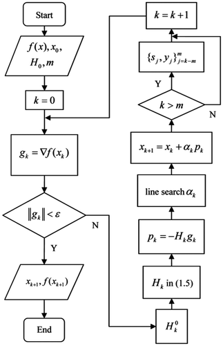
Within this algorithm, it is preferable to replace H₀ by $H_k^0={\mathit{\gamma }}_k{H}_0$ where ${\mathit{\gamma }}_k=y_k^T{s}_k/{∥y_k∥}^2$.[6] And the corresponding implement process can be seen in Figure 1.

Figure 1. The flow chart of L-BFGS method.

The conjugate gradient (CG) method coupled with adjoint equation,[13,14] similar to the L-BFGS method, is also a powerful minimization tool and represents a more general and straightforward approach. The solution strategy on which the CG method is based is essentially a regularisation procedure that is implemented iteratively by searching for the optimal minimum of the objective function expressing the deviation between the behaviour predicted by the direct (or forward) problem and that actually observed, namely the corresponding measured data, in which the number of iterations is chosen so that stable solutions are obtained for the inverse problem. The CG has already shown its potential for solving many kinds of inverse problems and been applied to many different applications.[15–17] Using this CG with adjoint equation, the minimization of the cost function for the solution of estimation of variable coefficient can be conveniently divided into several basic steps: (1) the solution of direct problem; (2) the solution of sensitivity problem; (3) the cost functional and the solution of adjoint problem; (4) the gradient equation; (5) the CG method for minimising the cost functional. We will present below the details of each of such steps. As a variant of the CG algorithm, a spectral conjugate gradient (SCG) method is first given by Birgin and Martinez [18]. In order to overcome the lack of positive definiteness of the matrix defining the search direction, Neculai Andrei later made a modification for the SCG based on the quasi-Newton BFGS updating formula,[19] which makes the SCG more efficient and robust in numerical experiments due to the introduction of the spectral gradient comparable to the L-BFGS method. Compared with the CG method, the convergence of the SCG is better than that of the classical CG because the SCG not only inherits the second-order information of the BFGS, but also preserves the characteristic feature of the classical CG method. So the modified SCG method is employed in this paper to carry out the estimation of variable coefficient D(x) based on the same test condition as used for the AdR-LBFGS. The idea of using the SCG in inverse problem is not new, see [20]. However, in view of the advantage of regularisation technique performed in the literature,[5] we are more interested here in combining the SCG with regularisation technique (called the AdR-SCG in the text) to ascertain whether adding regularisation term to the cost functional improves variable coefficient retrieval more than does the case where the regularisation term is not included in cost functional (called the NoR-SCG versus AdR-SCG). The main purposes of this paper are to design the whole frame of retrieval process for the variable coefficient D(x) based on the basic requirement of the SCG and explore the recovery of the variable coefficient D(x). In addition, we will see below that when noisy data are considered, the application of the regularisation technique in the cost functional is still necessary though the regularisation is implicitly built in the computational procedure of the SCG. The main contribution of this paper consists of: (1) providing the formulation of the SCG method combined with adjoint method. The most important components that need to be tackled carefully are focused on the determination of the choice of the step length and the descent direction. The former is deduced and then achieved numerically by solving the given sensitivity equation, and the latter is formulated by the spectral gradient. These two steps are the most expensive calculations in the minimization process; (2) performing some comparable numerical experiments between the SCG and the L-BFGS with respect to different data types (noise-free and noisy data, dense and sparse data) to illustrate the advantage of the SCG; (3) studying the effects of different forms of initial guess distributions, as well as various levels of noise, on the retrieval results.

The rest of this paper is organised as follows. In Section 2, we present a basic framework of the SCG solution strategy according to the basic steps just mentioned above. Then in Section 3, several numerical experiments are performed in different data types. And finally, we give some discussions and conclusions in Section 4. For the sake of ensuring the completeness of the SCG algorithm, some related contents established in the literature,[5] such as the numerical scheme of the direct problem, the adjoint problem, etc., are still to be placed here to use in the subsequent analysis.

2. The framework of SCG solution strategy to retrieve the model parameter

2.1. Numerical model of the direct problem

To develop a numerical scheme for the direct problem (1.1a)–(1.1c), we first discretize the spatial domain [0, l] to get Δx = l/M and the time domain to obtain Δt = τ/N, given two positive integers M and N (the total number of grid points in space and in time, respectively). And then let $u_j^n$ denote the state variable at every grid, i.e. $u_j^n=u(j\mathrm{\Delta }x,n\mathrm{\Delta }t)$, where j = 1, …, M − 1, n = 0, 1, …, N, according to the finite volume method, the following semi-implicit and implicit difference schemes over the domain $[0,l]\times [0,\mathit{\tau }]$ can be presented (for more details, please see [5]):(2.1.1) $$u_j^n-u_j^{n-1}=\frac{\mathrm{\Delta }t}{2\mathrm{\Delta }x}(u_{j-1}^{n-1}-u_j^{n-1})(u_j^{n-1}+u_{j-1}^{n-1})+\frac{\mathrm{\Delta }t}{\mathrm{\Delta }{x}^2}[D(j+1/2)(u_{j+1}^n-u_j^n)-D(j-1/2)(u_j^n-u_{j-1}^n)]$$(2.1.1) (2.1.2) $$u_j^n-u_j^{n-1}=\frac{\mathrm{\Delta }t}{2\mathrm{\Delta }x}(u_{j-1}^n-u_j^n)(u_j^n+u_{j-1}^n)+\frac{\mathrm{\Delta }t}{\mathrm{\Delta }{x}^2}[D(j+1/2)(u_{j+1}^n-u_j^n)-D(j-1/2)(u_j^n-u_{j-1}^n)]$$(2.1.2)

where D(x) is defined at semi-grid point, namely $D(j+1/2)=D(x_j+\frac{1}{2}\mathrm{\Delta }x)$. While the time step size used for time integration of the direct problem is dictated by the Courant-Friedrichs-Levy (CFL) condition to ensure stability.

Correspondingly, from the initial and boundary conditions, i.e. (1.1b) and (1.1c), we have(2.1.3a) $$u(x_j,0)=\mathit{\phi }(x_j)={\mathit{\phi }}_j$$(2.1.3a)

(2.1.3b) $$u(x_0,t_n)=u(x_M,t_n)=0.$$(2.1.3b)

once the initial value φ_j and diffusion coefficient D_j are specified, the solution $u_j^n$ is completely determined. The semi-implicit difference scheme is used for the numerical calculation of the state variable u(x, t), whereas the implicit difference scheme will be then used for the provision of simulated observation data in the consequent numerical experiments.

2.2. The sensitivity problem

The sensitivity problem, necessary for determining the optimal step size β involved in (2.4.1) and (2.4.2), can be derived directly from the semi-implicit difference scheme (2.1.1) assuming that the variable coefficient D(x) undergoes an increment ΔD(x), and the state variable u(x, t) changes by an amount Δu(x, t). Then, in order to obtain the sensitivity problem that satisfies the function Δu(x, t), u(x, t) is replaced by u(x, t) + Δu(x, t) and D(x) by D(x) + ΔD(x) in the direct problem (2.1.1), (2.1.3a), and (2.1.3b), subtracting from the original problem. The discrete sensitivity problem is then obtained below$$\mathrm{\Delta }{u}_j^n-\mathrm{\Delta }{u}_j^{n-1}=\frac{\mathrm{\Delta }t}{2\mathrm{\Delta }x}\left[(\mathrm{\Delta }{u}_{j-1}^{n-1}-\mathrm{\Delta }{u}_j^{n-1})(u_j^{n-1}+u_{j-1}^{n-1})+(u_{j-1}^{n-1}-u_j^{n-1})(\mathrm{\Delta }{u}_j^{n-1}+\mathrm{\Delta }{u}_{j-1}^{n-1})\right]+\frac{\mathrm{\Delta }t}{\mathrm{\Delta }{x}^2}\left[\mathrm{\Delta }{D}_{j+\frac{1}{2}}(u_{j+1}^n-u_j^n)+D_{j+\frac{1}{2}}(\mathrm{\Delta }{u}_{j+1}^n-\mathrm{\Delta }{u}_j^n)-\mathrm{\Delta }{D}_{j-\frac{1}{2}}(u_j^n-u_{j-1}^n)-D_{j-\frac{1}{2}}(\mathrm{\Delta }{u}_j^n-\mathrm{\Delta }{u}_{j-1}^n)\right]$$(2.2.1) $$\begin{array}{c}\mathrm{\Delta }{u}_j^0=0,(j=1,\dots ,M-1)\hfill \\ \mathrm{\Delta }u(x_0,t_n)=\mathrm{\Delta }u(x_M,t_n)=0\hfill \end{array}$$(2.2.1)

In this sensitivity problem, ΔD(x) is the only forcing function needed for the calculation of Δu. While the choice of ΔD(x) will be described later in the analysis.

2.3. The cost functional and the corresponding adjoint problem

Since the adjoint problem of the direct problem (1.1a)–(1.1c) depends on the choice of an inner product defined by the cost functional, we first give here the cost functional.

If D_j denotes the control variable, the discrepancy between the observation value ${\tilde{u}}_j^n$ and the state variable (model results) $u_j^n$ may be then defined by a cost functional of the form

(2.3.1) $$J[D]=\frac{1}{2}\sum _{n=0}^N\sum _{j=1}^{M-1}{(u_j^n-{\tilde{u}}_j^n)}^2+\frac{{\mathit{\gamma }}^2}{2}\sum _{j=1}^M\sum _{n=0}^N{D}_{j-1/2}{(u_j^n-u_{j-1}^n)}^2$$(2.3.1)

where γ is regularisation parameter. And the second term we add in J describes a priori constraint one would like the desired state function to be subject to. As suggested by the literature,[21–24] ill-posed problems can yield stable solution if sufficient a priori information about the true solution is available. The frequently used regularisation functional can be expressed as a term with differential operator, i.e. ${∥Lu∥}_2^2$, which varies according to the specific problem, may be ${\int }_0^T{\int }_{\mathrm{\Omega }}{\left|u\right|}^2\text{d}\mathrm{\Omega }\text{d}t$, ${\int }_0^T{\int }_{\mathrm{\Omega }}{\left|\mathit{\partial }u/\mathit{\partial }x\right|}^2\text{d}\mathrm{\Omega }\text{d}t$ or ${∥Lu∥}^2$, where L is a closed linear operator.[25] The effect of ${\int }_0^T{\int }_{\mathrm{\Omega }}{\left|u\right|}^2\text{d}\mathrm{\Omega }\text{d}t$ tends to seek for the minimum-norm solution and ${\int }_0^T{\int }_{\mathrm{\Omega }}{\left|\mathit{\partial }u/\mathit{\partial }x\right|}^2\text{d}\mathrm{\Omega }\text{d}t$, as a $H_0^1$-seminorm, makes the solution more stable by reducing the undesired oscillations during computational process. As a continuous version of the second term appearing in cost functional (2.3.1), from the point of view of physics, the term ${\int }_0^T{\int }_{\mathrm{\Omega }}D(x){\left|\mathit{\partial }u/\mathit{\partial }x\right|}^2\text{d}\mathrm{\Omega }\text{d}t$ is essentially a component part of energy functional derived in variational setting from Equations (1.1a)–(1.1c). Addition of this term in cost functional can be therefore equivalent to perform a bounded constraint of energy seminorm associated with D(x) due to nonhomogeneous medium. As for the ${\int }_0^T{\int }_{\mathrm{\Omega }}{\left|dD/dx\right|}^2\text{d}\mathrm{\Omega }\text{d}t$ or ${\int }_0^T{\int }_{\mathrm{\Omega }}{\left|D(x)\right|}^2\text{d}\mathrm{\Omega }\text{d}t$, it is feasible in mathematics to regard them as a constraint, but their physical meaning is unknown. So it is natural to select ${\int }_0^T{\int }_{\mathrm{\Omega }}D(x){\left|\mathit{\partial }u/\mathit{\partial }x\right|}^2\text{d}\mathrm{\Omega }\text{d}t$ as regularisation stable functional in the current study. It is shown experimentally later that imposing such a priori constraint leads a stable solution within a suitable noise range.

From the definition of the cost functional (2.3.1), J depends only on the control variable D(x) through the state variables $u_j^n$, j = 1, …, M − 1, which are solutions of the forward problem defined by Equations (2.1.1), (2.1.3a), and (2.1.3b). If the observations ${\tilde{u}}_j^n$ and the initial value φ_j are known, diffusion coefficient D_j can be the retrieved. So the current inverse problem can be regarded as an optimal control problem of finding the variable coefficient D_j.

Having the cost functional in hand, through a series of calculation, the following adjoint equations and adjoint boundary conditions are obtained$${\mathit{\lambda }}_j^n={\mathit{\lambda }}_j^{n+1}-\frac{\mathrm{\Delta }t}{\mathrm{\Delta }x}{u}_j^n({\mathit{\lambda }}_j^{n+1}-{\mathit{\lambda }}_{j+1}^{n+1})+\frac{\mathrm{\Delta }t}{\mathrm{\Delta }{x}^2}[D_{j-1/2}{\mathit{\lambda }}_{j-1}^{n+1}-(D_{j+1/2}+D_{j-1/2}){\mathit{\lambda }}_j^{n+1}+D_{j+1/2}{\mathit{\lambda }}_{j+1}^{n+1}]+(u_j^n-{\tilde{u}}_j^n)+{\mathit{\gamma }}^2[D_{j-1/2}(u_j^n-u_{j-1}^n)-D_{j+1/2}(u_{j+1}^n-u_j^n)]$$(2.3.2) $$\begin{array}{c}{\mathit{\lambda }}_j^{N+1}=0,{\mathit{\lambda }}_0^n={\mathit{\lambda }}_M^n=0\\ n=N,N-1,\dots ,1,0;j=1,2,\dots ,M-1\end{array}$$(2.3.2)

where $\mathit{\lambda }$ stands for the adjoint variable that is necessary for the computation of the following gradients of the cost functional with respect to D(x):(2.3.3) $$\mathrm{\nabla }J[D]=\frac{\mathit{\partial }J}{\mathit{\partial }{D}_{j-1/2}}=\frac{\mathrm{\Delta }t}{\mathrm{\Delta }{x}^2}\sum _{n=1}^N(u_j^{n-1}-u_{j-1}^{n-1})({\mathit{\lambda }}_{j-1}^n-{\mathit{\lambda }}_j^n)+\frac{{\mathit{\gamma }}^2}{2}\sum _{n=0}^N{(u_j^n-u_{j-1}^n)}^2,j=1,2,\dots ,M$$(2.3.3)

2.4. The computational algorithm of SCG method

In this subsection, for the determination of variable coefficient D(x), we consider the recurrence equation(2.4.1) $$D^{k+1}=D^k-{\mathit{\beta }}^k{d}^k,k=0,1,2,\dots ,$$(2.4.1)

where $D^T=(D_{1/2},D_{3/2},\cdots ,D_{M-1/2})=(D_{j-1/2}),j=1,2,\dots ,M$, and D⁰ is a guess value.

By replacing $u_j^n$ by $u_j^n(D^k-{\mathit{\beta }}^k{d}^k)$, the objective functional (2.3.1) becomes(2.4.2) $$J[D^{k+1}]=\frac{1}{2}\sum _{n=0}^N\sum _{j=1}^{M-1}{[u_j^n(D^k-{\mathit{\beta }}^k{d}^k)-{\tilde{u}}_j^n]}^2+\frac{{\mathit{\gamma }}^2}{2}\sum _{j=1}^M\sum _{n=0}^N{D}_{j-1/2}{[u_j^n(D^k-{\mathit{\beta }}^k{d}^k)-u_{j-1}^n(D^k-{\mathit{\beta }}^k{d}^k)]}^2$$(2.4.2)

The $u_j^n(D^k-{\mathit{\beta }}^k{d}^k)$ can be linearized with a Taylor series expansion below(2.4.3) $$u_j^n(D^k-{\mathit{\beta }}^k{d}^k)\approx u_j^n(D^k)-{\mathit{\beta }}^k\frac{\mathit{\partial }{u}_j^n}{\mathit{\partial }{D}^k}{d}^k$$(2.4.3)

Let d^k = ΔD^k, Equation (2.4.3) above becomes

(2.4.4) $$u_j^n(D^k-{\mathit{\beta }}^k{d}^k)\approx u_j^n(D^k)-{\mathit{\beta }}^k\mathrm{\Delta }{u}_j^n$$(2.4.4)

By substituting Equation (2.4.4) into Equation (2.4.2), and then the minimization of the cost functional (2.4.2) with respect to β^k is performed to yield the following expression for the step length(2.4.5) $${\mathit{\beta }}^k=\frac{{\sum }_{n=0}^N{\sum }_{j=1}^{M-1}{(\mathrm{\Delta }u)}_j^n(u_j^n-{\tilde{u}}_j^n)+{\mathit{\gamma }}^2{\sum }_{n=0}^N{\sum }_{j=1}^M{D}_{j-1/2}(u_j^n-u_{j-1}^n)[{(\mathrm{\Delta }u)}_j^n-{(\mathrm{\Delta }u)}_{j-1}^n]}{{\sum }_{n=0}^N{\sum }_{j=1}^{M-1}{[{(\mathrm{\Delta }u)}_j^n]}^2+{\mathit{\gamma }}^2{\sum }_{n=0}^N{\sum }_{j=1}^M{D}_{j-1/2}{[{(\mathrm{\Delta }u)}_j^n-{(\mathrm{\Delta }u)}_{j-1}^n]}^2}$$(2.4.5)

And the calculation of ${(\mathrm{\Delta }u)}_j^n$ will be presented by solving the sensitivity problem (2.2.1) forced by (ΔD)^k = d^k.

Let $s^{k-1}=D^k-D^{k-1},y^{k-1}=\mathrm{\nabla }J[D^k]-\mathrm{\nabla }J[D^{k-1}]$, then we obtain the following spectral gradient [13](2.4.6) $${\mathit{\theta }}^k=\frac{{(s^{k-1})}^T{s}^{k-1}}{{(y^{k-1})}^T{s}^{k-1}},$$(2.4.6)

where ${(y^{k-1})}^T{s}^{k-1}>0$. So the direction of descent, d^k, can be provided by(2.4.7) $$\begin{array}{cc}{d}^0=-\mathrm{\nabla }J[D^0],\hfill & \text{for}k=0\hfill \\ d^k=-{\mathit{\theta }}^k\mathrm{\nabla }J[D^k]+{\mathit{\theta }}^k\frac{\mathrm{\nabla }J{[D^k]}^T{s}^{k-1}}{{(y^{k-1})}^T{s}^{k-1}}{y}^{k-1}-[\left(1+{\mathit{\theta }}^k\frac{{(y^{k-1})}^T{y}^{k-1}}{{(y^{k-1})}^T{s}^{k-1}}\right)\frac{\mathrm{\nabla }J{[D^k]}^T{s}^{k-1}}{{(y^{k-1})}^T{s}^{k-1}}\hfill \\ -{\mathit{\theta }}^k\frac{\mathrm{\nabla }J{[D^k]}^T{y}^{k-1}}{{(y^{k-1})}^T{s}^{k-1}}]s^{k-1}\hfill & \text{for}k\ge 1.\hfill \end{array}$$(2.4.7)

From the above, we see that the update formulations of direction d^k are well done using a memoryless BFGS quasi-Newton updating expression.

2.5. The stopping criterion

The most widespread stopping rule for iterative methods is the discrepancy principle when a priori knowledge of the standard deviation of the measurement errors is known in advance. If a small number ɛ is specified, then the stopping criterion of recurrent process can be obtained as follows:

(2.5.1) $$J[D^{k+1}]<\mathit{\epsilon }$$(2.5.1)

When the measurements are regarded as errorless, the tolerance ɛ can be chosen as a sufficiently small number. When the measurements contain random errors, say, σw, where ω is the random variable and σ is the standard deviation of the measurement error, then according to Equation (2.3.1), ɛ can be taken approximately as $(N+1)(M-1){\mathit{\sigma }}^2/2$, where (N + 1)(M − 1) represents the total number of observation data.

If the cost functional J has a minimum value that is larger than ɛ, the iterations are stopped either when the cost function J satisfies the following condition:

(2.5.2) $$J[D^k]-J[D^{k+1}]<{\mathit{\epsilon }}_p$$(2.5.2)

where ɛ_p is a prescribed small number or when a maximum number of the iteration counter reaches 800. The latter is the same as used in L-BFGS reported in Ref. [5]. The motivation for adding such an extra stopping iteration 800 here is to better understand what happens in difference between the SCG and the L-BFGS. The results shown later in the case of H without noise reveal that when the iteration reaches 800, the SCG can lead to an improvement of three orders of magnitude in accuracy compared to the L-BFGS. Actually, the stopping iteration should have been taken much smaller than 800. In real application, when a typical minimization is encountered, which is characterised by a fast decrease in the cost function during the first few tens of iterations, followed by a slowly decreasing (almost flat) behaviour, even if the solution keeps on getting better during this slow convergence period, practical considerations should prompt us to stop the minimization.

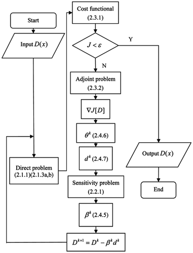
The whole computational algorithm of the SCG method combining with adjoint equation can be expressed as in Figure 2.

Figure 2. The flow chart for the whole computational algorithm of SCG.

3. Numerical results

3.1. The true value of state variable and observation

In order to check the feasibility of the SCG and implement the comparisons between the NoR-SCG, AdR-SCG and AdR-LBFGS, a set of test conditions must be predefined. Considering $\mathit{\tau }=0.1$, l = 1, N = 100 and M = 20, for a given initial state and specific diffusion coefficient(3.1.1) $${\mathit{\phi }}^t(x_j,0)=sin(\mathit{\pi }{x}_j),D^p(x_j)=x_j^2,j=1,\dots ,M-1$$(3.1.1)

and performing the time integration of the model (2.1.2) generates a set of ‘true data’, $u_j^n,j=1,\dots ,19;n=1,\dots ,100$. Here, the superscript ‘t’ stands for the truth, and ‘p’ is the exact solution. Taken from ‘true data’, the corresponding observation is then as follows:

(1)	Dense observation data(3.1.2) $$H=\{\left.{\tilde{u}}_j^n=u_j^n\right|j=1,\dots ,19;n=1,\dots ,100\};$$(3.1.2) which coincides with the grid point of the numerical computation;
(2)	Sparse observation data are denoted by $\overline{H}$ (obtained at every 10 time steps) and $\overline{\overline{H}}$ (available at every 50 time steps) in this study.

They will be stored for preparing for the numerical experiments shown in what follows. When some noise needs to be considered in observation data, the corresponding experimental data can be generated by adding an error term σw to the simulated observation data mentioned in (1) and (2) above, respectively.

3.2. Numerical experiments

Before proceeding to the numerical experiments, we first assume that we have imperfect knowledge of the diffusion coefficient through an initial guess, D^g(x), with the resolution equal to the one that helps us define the true state as in Section 3.1:

(3.2.1) $$D^g(x)=x^2+0.1$$(3.2.1)

To further quantify the differences between the guesses and the true state (the priori knowledge), we use the L² norm(3.2.2) $${∥f∥}_{L^2}={\left({\int }_0^1{f}^{2}dx\right)}^{1/2}$$(3.2.2)

to define the relative error at iteration m,

(3.2.3) $$e_m^D={∥D_m^{}-D^p∥}_{L^2}/{∥D^p∥}_{L^2},m=0,1,\dots$$(3.2.3)

Hence, the initial differences just before the startup of numerical experiments can be characterised by the relative error: $e_0^D=0.2238$.

3.2.1. Dense data (noise-free and noisy data)

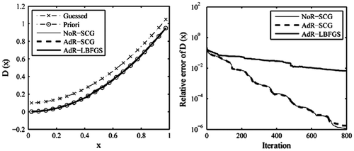
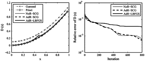
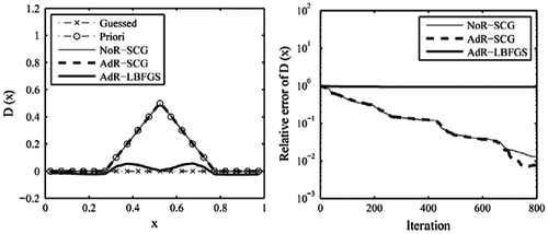
We first verify the validity of the SCG method in this paragraph through reconstructing the variable coefficient appearing in (3.1.1) with noise-free observation data H (3.1.2). Starting from the initial guess of D(x) (3.2.1), when the iteration counts reaches 800, the iterative process is terminated in advance though this process is still to proceed according to the requirement of the stopping criterion (2.5.1) or (2.5.2). The results are presented in Figure 3. Compared with the true (priori) variable coefficient, the AdR-LBFGS, the NoR-SCG and the AdR-SCG all provide a quite good recovery result. Their resulting error levels become: $e_k^D=6.6000\times {10}^{-3}$, $e_k^D=1.1056\times {10}^{-6}$ and $e_k^D=1.7861\times {10}^{-6}$, respectively. This illustrates the feasibility and validity of the SCG method. Again, it is seen that the NoR-SCG and AdR-SCG solutions are nearly identical, suggesting that it is not necessary to adopt the regularisation technique in cost functional for SCG when reconstructing the variable coefficient in the case of noise-free observation data H.

Figure 3. The recovered results based on the observation data-set H.

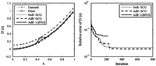
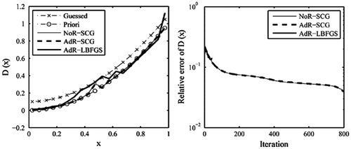
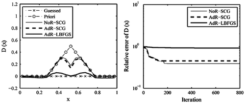
In practical operations, however, the available observations are often contaminated by some noise. So a level of uncertainty for the whole observation data H is taken into account. Here, a random Gaussian noise with mean of 0 and a standard deviation of 0.01 (i.e. σ = 0.01) is added to the simulated observation fields H to investigate the anti-noise ability of the SCG. We are still to select iterative counts 800 as termination condition, and the test results are indicated in Figure 4. It is clear in such situation that the iterative process corresponding to the AdR-LBFGS stops automatically in advance at iteration 221, and the relative error is only brought down to $e_k^D=5.8500\times {10}^{-2}$, leaving no room for making further improvement. But for alternative approach, the NoR-SCG or the AdR-SCG, the corresponding relative errors undergo a fast decrease during the first iterations of about 230, followed by a slowly decreasing (almost flat). That is to say, the first iterations of about 230 contribute dominant part to the current inversion results, suggesting that the iterative process should be stopped at iteration 230, rather than at iteration 800. From the comparison between Figures 3 and 4, we can see that affected by noise, the recovery result of variable coefficient D(x) using the AdR-LBFGS is somewhat coarser than that using either the NoR-SCG or the AdR-SCG, but still acceptable. At the same time, it is found from Figure 4 that despite noise added to databases H, the derivative results from the two SCGs have very good stability. Particularly, for the AdR-SCG, the retrieved result has higher precision, which is largely due to the consideration of regularisation term in cost function (2.3.1), i.e. γ ≠ 0.

Figure 4. The recovered results based on the observation data-set H with noise.

In a word, these three methods all can provide satisfying recovery result of variable coefficient D(x) using the dense database H, whether noisy or noise-free. When noise arises in the observation data, the impact of the regularisation technique on estimating variable coefficient is positive and obvious.

3.2.2. Sparse data (noise-free and noisy data)

In general, we do not have observations of the state variables at every time step. The observations used in practical operation are sparse in time, i.e. not necessarily available at every time step. So in this subsection, we investigate whether we still obtain a good solution if we use fewer observations. Here, two kinds of database of observation, $\overline{H}$ and $\overline{\overline{H}}$, described previously in Section 3.1, are used for retrieving the variable coefficient. Given an initial guess (3.2.1), the termination condition of the iterative process is that the iterations reach 800, then recovery results for D(x) based on two kinds of observation data, $\overline{H}$ and $\overline{\overline{H}}$, are shown in Figures 5 and 6, respectively. 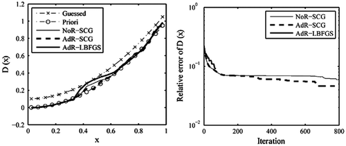It can be seen that for the applications of the observation set, $\overline{H}$ and $\overline{\overline{H}}$, the retrieval result of D(x) caused by either the AdR-LBFGS only or the SCG only leads to a decrease in the relative error of D(x). 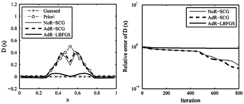In the case of the AdR-LBFGS, the resulting L² error level 3.4000 × 10⁻² with $\overline{H}$ in Figure 5 is much better than 1.4300 × 10⁻¹ with $\overline{\overline{H}}$ in Figure 5 whose recovery result becomes at this time unacceptable because the corresponding iterative process stops earlier at iterations 42. Whereas in the case of the SCG, the situation is entirely different, and the resulting error levels are 5.9000 × 10⁻³ (NoR-SCG), 5.5000 × 10⁻³ (AdR-SCG) with $\overline{H}$, and 4.1000 × 10⁻² (NoR-SCG), 3.9500 × 10⁻² (AdR-SCG) with $\overline{\overline{H}}$. So there are considerable improvements compared with the results of the AdR-LBFGS with either $\overline{H}$ or $\overline{\overline{H}}$. It can also be seen that the estimated result of the SCG with $\overline{\overline{H}}$ can be comparable to that of AdR-LBFGS with $\overline{H}$, which illustrates that the performance of the SCG is better than that of the AdR-LBFGS. This is mainly due to the fact: first, the SCG adopts optimal step length at each iteration, calculated via the proposed sensitivity problem, and second, the SCG itself belongs to the iterative regularisation class. In addition, we find that decreasing the observation data (sparse time sampling) leads to a loss of accuracy in the estimation of variable coefficient, which poses considerable difficulties to some extent in retrieving variable coefficient by whatever tool, particularly in the present AdR-LBFGS. And the AdR-SCG is advantageous, we see, in the case of $\overline{H}$ and $\overline{\overline{H}}$, but not as obvious as expected.

Figure 5. The recovered results based on the observation data-set $\overline{H}$.

Figure 6. The recovered results based on the observation data-set $\overline{\overline{H}}$.

As mentioned in Section 3.2.1, when using the SCG method to retrieve D(x) with observation data contaminated by noise, it is helpful to consider the regularisation technique for enhancing the recovery accuracy. To illustrate this tendency, here we impose upon the sparse observation database $\overline{H}$ and $\overline{\overline{H}}$ the same noise as one involved in Section 3.2.1. 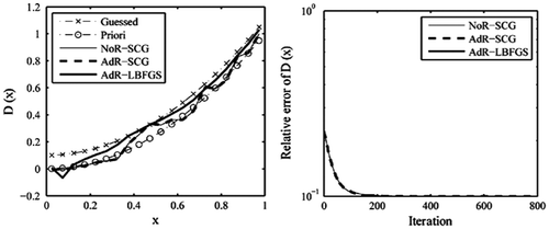In the case of $\overline{H}$ with noise, when we terminate the iterative process at iteration 800, the variable coefficient D(x) has been corrected significantly using either the NoR-SCG or the AdR-SCG (see Figure 7). In particular, the recovery effect of D(x) using AdR-SCG is more obvious and is remarkablely close to the true (Priori) D^p(x). While for the AdR-LBFGS, the corrected result of D(x) does not allow us to reach error levels as small as the one obtained even using the NoR-SCG method. 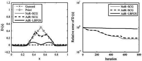In the case of $\overline{\overline{H}}$ with noise, the addition of noise leads directly to an imperfect recovery result. Even if for the AdR-SCG, its anti-noise ability is also hindered by current noise level (see Figure 8). To what extent reducing the imposed noise level can help alleviate this situation deserves a further investigation.

Figure 7. The recovered results based on the observation data-set $\overline{H}$ with noise.

Figure 8. The recovered results based on the observation data-set $\overline{\overline{H}}$ with noise.

In order to investigate the effect of different levels of noise on retrieval results, we introduce Table 1 to present a quantitative comparison of the SCG and L-BFGS for the data with and without noise. The addition of noise to the data-set has a noticeable impact on the performance of the SCG and L-BFGS method. As expected, increasing the measurement errors leads to a loss of accuracy in the estimation of the variable coefficient. An obvious trend can be readily observed, i.e. the sparser the available data-set becomes, the smaller the range of the noise level gets. However, from the results of at least two orders of magnitude shown in Table 1, the SCG behaves better than the L-BFGS. We notice that the noise level range required in H is from 0 up to about 0.07 in the case of the SCG, while in the case of the L-BFGS, the noise level imposed on H is taken only from 0 to about 0.05. Even though with the results of identical order of magnitude in the same row in Table 1, the SCG also works better than the L-BFGS. This implies that the anti-noise ability of SCG method is superior to that of the L-BFGS method. It can be so stated that with the L-BFGS method, the relative error of variable coefficient obtained using the data with different levels of noise never make it to the accuracy that we get with the SCG method to a large extent. Moreover, it should be noted that implementing the algorithm SCG needs to run the model of sensitivity equation (2.2.1) for the purpose of calculating step length (2.4.5) at each iterative step, which will spend much more time compared with the L-BFGS method. This can be observed by the listed CPU time in Table 1. This may not be an active factor for the SCG to make further practical application such as the large-scale problem. However, with the fast development of the reduced-order techniques,[26,27] it is also possible to use the SCG method in the framework of inverse problem of reduced-order model. This issue still needs to be addressed in separate studies.

Table 1. Effects of different levels of noise on the retrieval result using the SCG and L-BFGS method.

Data			Method
			NoR-SCG			AdR-SCG			AdR-LBFGS
			Iter.	CPU/s	Error	Iter.	CPU/s	Error	Iter.	CPU/s	Error
H	Without noise		800	25.1682	1.1056E-6	800	23.8581	1.7861E-6	800	15.0800	6.6000E-3
	Noise level	0.01	800	25.4186	2.1359E-2	800	24.4783	1.9296E-2	221	5.2741	5.8500E-2
		0.03	800	25.2125	6.2176E-2	800	24.5845	5.3894E-2	265	10.0257	6.7413E-2
		0.05	800	25.6903	7.7555E-2	800	23.9358	7.6143E-2	63	1.9440	8.5066E-2
		0.07	800	25.9120	9.4606E-2	800	23.9685	8.7593E-2	36	0.8866	1.1528E-1
		0.08	800	26.2956	1.1579E-1	800	23.9792	1.1488E-1	25	0.5013	1.3307E-1
$\overline{H}$	Without noise		800	25.1314	5.9000E-3	800	24.5823	5.5000E-3	800	23.0898	3.4000E-2
	Noise level	0.01	800	24.8626	5.8993E-2	800	23.2076	4.6337E-2	70	2.1387	9.1872E-2
		0.02	800	24.1536	1.0504E-1	800	23.8342	1.0617E-1	102	3.1797	9.3933E-2
		0.03	800	24.8353	1.9087E-1	800	22.9491	1.7027E-1	57	1.6880	9.6937E-2
$\overline{\overline{H}}$	Without noise		800	24.8658	4.1000E-2	800	24.3530	3.9500E-2	42	1.5728	1.4300E-1
	Noise level	0.007	800	24.8980	8.5541E-2	800	24.4547	8.7775E-2	30	1.1596	1.2367E-1
		0.009	800	24.3269	9.8685E-2	800	23.9578	9.8870E-2	8	0.8236	1.8503E-1
		0.01	800	24.2218	9.9909E-2	800	25.1796	9.9911E-2	0	0.0560	2.2384E-1

Note: Iter. is short for iteration and the CPU time is obtained with the Core i3-2100 CPU(3.10 GHz) and Windows XP operating system.

In order to further assess the retrieval ability of the algorithm SCG and L-BFGS in the current work, the diffusion coefficient reconstruction for a corner function is also considered. For example, a typical triangle function is adopted here$$D^p(x)=\left\{\begin{array}{cc}0,\hfill & 0<x\le 0.25\hfill \\ 0.5\left[1-\frac{|x-0.525|}{0.25}\right],\hfill & 0.25<x\le 0.8\hfill \\ 0,\hfill & 0.8\le x<1\hfill \end{array}\right.$$

So the observation data-sets H and $\overline{H}$, as classified in the case of D^p(x) = x², are changed into H_T and ${\overline{H}}_T$, respectively. And the initial guess is set to be zero, i.e.

Figure 9. The recovered results based on the observation data-set H_T.

Figure 10. The recovered results based on the observation data-set H_T with noise level 0.01.

Figure 11. The recovered results based on the observation data-set ${\overline{H}}_T$.

Figure 12. The recovered results based on the observation data-set ${\overline{H}}_T$ with noise level 0.01.

$$D^g=0.$$

The results are shown below:

(1)	Case of HT (Figures 9 and 10).
(2)	Case of ${\overline{H}}_T$ (Figures 11 and 12).

For the current test case, it is shown that the retrieval results of SCG method are also better than that of L-BFGS method. In the case of data-set H_T without error, the SCG result matches well with the true solution. When the observation data become sparse or a level of error is considered, the obtained results will be heavily affected. Despite the peak value of the true function could not be exactly recovered, we see that the locations of the discontinuities in the first derivative of D(x) were still resolved by these two methods.

3.2.3. The effect of different initial guesses

In practical application, the variable coefficient cannot be known in advance and no information is provided. In this subsection, we will study the effect of different initial guesses distribution on the retrieval validation. With this objective in mind, several shapes of initial guesses are taken into account as follows:

(1)	Constant function$$D^g(x)=0.1$$
(2)	Sinusoidal-like function$$D^g(x)=\left\{\begin{array}{cc}0,\hfill & 0<x\le 0.25\hfill \\ 0.5\left[1-\frac{{(x-0.5)}^2}{0.{25}^2}\right],\hfill & 0.25<x<0.8\hfill \\ 0,\hfill & 0.8\le x<1\hfill \end{array}\right.$$
(3)	Step function$$D^g(x)=\left\{\begin{array}{cc}0,\hfill & 0<x\le 0.25\hfill \\ 0.5,\hfill & 0.25<x<0.8\hfill \\ 0,\hfill & 0.8\le x<1\hfill \end{array}\right.$$
(4)	Triangle function $$D^g(x)=\left\{\begin{array}{cc}0,\hfill & 0<x\le 0.25\hfill \\ 0.5\left[1-\frac{|x-0.525|}{0.25}\right],\hfill & 0.25<x\le 0.8\hfill \\ 0,\hfill & 0.8\le x<1\hfill \end{array}\right.$$

We see that the initial guess distributions above have nothing to compare with the true variable coefficient below

$$D^p(x)=x^2$$

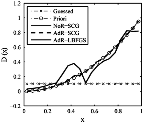
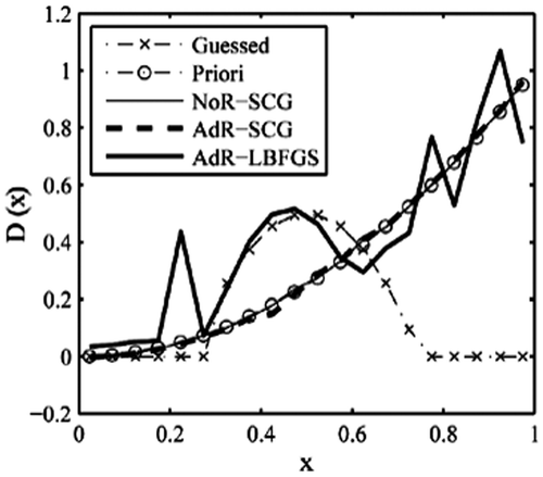
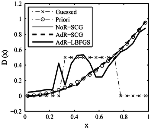
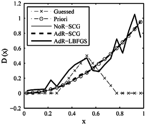
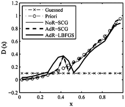
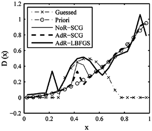
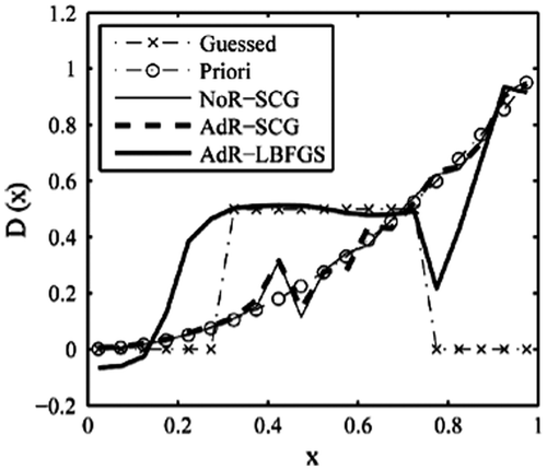
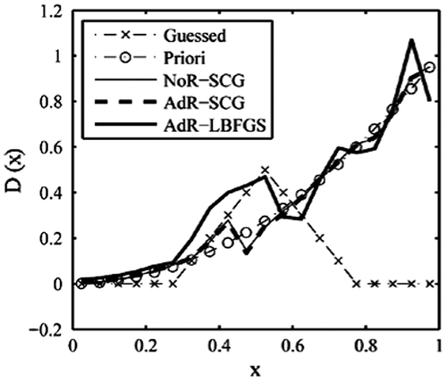
The inverse solutions obtained with different methods are presented in Figures 13–20. The computational process is done using the data with noise. The data types used here are H and $\overline{H}$, and the attached noise level is 0.01, respectively. It is sufficient if we want to show the significant difference between the SCG and L-BFGS in dealing with the different initial guess distributions.

1.	Case of H with noise level 0.01 (Figures 13–16).
2.	Case of $\overline{H}$ with noise level 0.01 (Figures 17–20).

Figure 13. Retrieval results with constant function (1).

Figure 14. Retrieval results with sinusoidal-like function (2).

Figure 15. Retrieval results with step function (3).

Figure 16. Retrieval results with triangle function (4).

Figure 17. Retrieval results with constant function (1).

Figure 18. Retrieval results with sinusoidal-like function (2).

Figure 19. Retrieval results with step function (3).

Figure 20. Retrieval results with triangle function (4).

By referring to the above testing examples, we see that using different initial guess distribution has impact on the retrieval results. However, this effect is very great in the L-BFGS method and much less in the SCG method. So, the SCG method has advantages over the L-BFGS method.

4. Conclusions

In the current study, the problem of retrieving variable coefficient for a nonlinear convection–diffusion equation is revisited in the case of sparse observation data in time sampling. The used inversion tools include the SCG method and the AdR-LBFGS applied previously in the literature.[5] In order to overcome the difficulties caused by noise, the regularisation technique is reconsidered in combination with SCG. To verify its validity, the SCG method is further splitted into two cases: the SCG with no regularisation term in the cost functional (termed NoR-SCG) and the SCG with a regularisation term integrated into the cost functional (termed AdR-SCG). The whole frame of calculating the inverse solution is designed according to the basic requirement of the SCG algorithm. For verifying the potential of these three methods with respect to retrieving variable coefficient, the comparisons between them are carried out using different data types (noise-free and noisy data, dense and sparse data). The recovery results show that the AdR-LBFGS method is easily affected by the change of the used observation data, and the SCG method, either NoR-SCG or AdR-SCG, has a relatively good stability which provides better effects than does the AdR-LBFGS method. In particular, when considering $\overline{H}$ with noise, the anti-noise ability of the SCG method is strengthened owing to the addition of regularisation term to the cost function which make AdR-SCG exhibit more obvious advantage over NoR-SCG. When it comes to the case of $\overline{\overline{H}}$ with noise, the NoR- and AdR-SCG do not provide us with desired inverse solution as obtained with noise-free $\overline{\overline{H}}$, see Figure 7. This reminds us that when using sparse observation data such as $\overline{\overline{H}}$ to retrieve the variable coefficient by the SCG method, special attention should be paid to the level of noise attached to the sparse observation data which is probably to prevent the success of the SCG method. When observation data sampling in time become sparse to some degree, apart from improving the inversion tool itself, keeping the noise level within a reasonable level is also helpful for ensuring a satisfying recovery effect.

The results above are promising, which can be viewed as a first step towards solving practical optimal control problem. More work, such as searching for a better regularisation technique and evaluating the performance of the SCG method with sparse observation data sampling in different spatial locations, rather than in time only and so on, remains to be done in separate study.

Acknowledgement

The authors are very grateful to the anonymous reviewers for carefully reading this manuscript and for their constructive suggestions which have improved the paper very much. Also, we would like to thank Editor-in-Chief, Professor George Dulikravich for managing the review process for this paper.

Additional information

Funding

This work is supported by the National Natural Science Foundation of China [grant number 41375115] and the Funding of Jiangsu Innovation Program for Graduate Education [grant number CXZZ12-0503].

References

- Nilssen TK, Tai XC. Parameter estimation with the augmented Lagrangian method for a parabolic equation. J. Optim. Theory Appl. 2005;124:435–453.10.1007/s10957-004-0944-y
- Huang SX, Han W, Wu RS. Theoretical analyses and numerical experiments of variational assimilation for one-dimensional ocean temperature model with techniques in inverse problems. Sci. Chin. Ser. D: Earth Sci. 2004;47:630–638.10.1360/02yd0195
- Engl HW, Zou J. A new approach to convergence rate analysis of Tikhonov regularization for parameter identification in heat conduction. Inverse Probl. 2000;16:1907–1923.10.1088/0266-5611/16/6/319
- Keung YL, Zou J. Numerical identifications of parameters in parabolic systems. Inverse Probl. 1998;14:83–100.10.1088/0266-5611/14/1/009
- Wang Y, Tao S. Application of regularization technique to variational adjoint method: a case for nonlinear convection–diffusion problem. Appl. Math. Comput. 2011;218:4475–4482.10.1016/j.amc.2011.10.028
- Liu DC, Nocedal J. On the limited memory BFGS method for large scale optimization. Math. Program. 1989;45:503–528.10.1007/BF01589116
- Jiang L, Douglas CC. An analysis of 4D variational data assimilation and its application. Computing. 2009;84:97–120.10.1007/s00607-008-0022-7
- Broyden CG. The convergence of a class of double-rank minimization algorithms 1. General considerations. IMA J. Appl. Math. 1970;6:76–90.10.1093/imamat/6.1.76
- Fletcher R. A new approach to variable metric algorithms. Comput. J. 1970;13:317–322.10.1093/comjnl/13.3.317
- Goldfarb D. A family of variable metric methods derived by variational means. Math. Comput. 1970;24:23–26.10.1090/S0025-5718-1970-0258249-6
- Shanno DF. Conditioning of quasi-Newton methods for function minimization. Math. Comput. 1970;24:647–656.10.1090/S0025-5718-1970-0274029-X
- Cacuci DG, Navon IM, Ionescu-Bujor M. Computational methods for data evaluation and assimilation. Boca Raton (FL): CRC Press; 2014.
- Jarny Y, Ozisik M, Bardon J. A general optimization method using adjoint equation for solving multidimensional inverse heat conduction. Int. J. Heat Mass Transfer. 1991;34:2911–2919.10.1016/0017-9310(91)90251-9
- Alifanov OM. Inverse heat transfer problem. Berlin: Springer; 1994.10.1007/978-3-642-76436-3
- Huang C-H, Chen K-Y. An iterative regularization method for inverse phonon radiative transport problem in nanoscale thin films. Int. J. Numer. Meth. Eng. 2007;69:1499–1520.10.1002/(ISSN)1097-0207
- Chiwiacowsky LD, de Campos Velho HF. Different approaches for the solution of a backward heat conduction problem. Inverse Probl. Eng. 2003;11:471–494.10.1080/1068276031000098027
- Bozzoli F, Rainieri S. Comparative application of CGM and Wiener filtering techniques for the estimation of heat flux distribution. Inverse Probl. Sci. Eng. 2011;19:551–573.10.1080/17415977.2010.531466
- Birgin E, Martinez JM. A spectral conjugate gradient method for unconstrained optimization. App. Math. Optim. 2001;43:117–128.10.1007/s00245-001-0003-0
- Andrei N. Scaled conjugate gradient algorithms for unconstrained optimization. Comput. Optim. Appl. 2007;38:401–416.10.1007/s10589-007-9055-7
- Wong JC-F, Xie J-L. Inverse determination of a heat source from natural convection in a porous cavity. Comput. Fluid. 2011;52:1–14.10.1016/j.compfluid.2011.07.013
- Hansen PC. Rank-deficient and discrete ill-posed problems. Philadelphia, PA: SIAM; 1998.10.1137/1.9780898719697
- Orlande HRB, Olivier F, Maillet D, Cotta RM. Thermal measurements and inverse techniques. New York: Taylor and Francis; 2011.
- Tichonov AN, Arsenin VY. Solution of ill-posed problems. Washington, DC: Winston; 1977.
- Bozzoli F, Cattani L, Rainieri S, Viloche Bazan FS, Borges LS. Estimation of the local heat-transfer coefficient in the laminar flow regime in coiled tubes by the Tikhonov regularisation method. Int. J. Heat Mass Transfer. 2014;72:352–361.10.1016/j.ijheatmasstransfer.2014.01.019
- Heinz WE, Hanke M, Neubauer A. Regularization of inverse problems. Kluwer Academic: Dordrecht; 1996.
- Vermeulen PTM, Heemink AW. Model-reduced variational data assimilation. Monthly Weather Review. 2006;134:2888–2899.10.1175/MWR3209.1
- Juan D, Navon IM, Zhu J, Fang F, Alekseev AK. Reduced order modeling based on POD of a parabolized Navier–Stokes equations model II: trust region POD 4DVAR data assimilation. Comput. Math. Appl. 2013;65:380–394.