Determination of sorption isotherm based on the measurements of contaminant outflow

Abstract

In this paper, we present a method for determining the sorption isotherm from experimental measurements. The sorption isotherm is not assumed to be a member of any specific finite dimensional class (e.g. Freundlich isotherm, Langmuir isotherm). Instead, an infinite-dimensional space of functions is considered with limited a priori assumptions (e.g. smoothness, monotonicity). Consequently, we face a more challenging problem compared to the finite-dimensional case, in which only few tuning parameters need to be determined. We consider the case of flow of the contaminated water into the unsaturated porous media sample; we assume that the data are collected at the outflow. The sorption isotherm is determined in an iterative way. We minimize the cost functional reflecting the discrepancy between measured and computed data. In doing so, we use the Gateaux differential to obtain the direction of descent.

Keywords:

• Gateaux differential
• unsaturated flow
• sorption isotherm
• numerical modelling
• optimization

AMS Subject Classifications:

• 49M25
• 65K10
• 76S05
• 90C90

1. Introduction

The protection of clean underground water in reservoirs is of great environmental importance and has received much attention also in the mathematical modelling community. In last decades, a significant progress has been achieved (see e.g. [1, 2]). Precise mathematical models can describe realistically the flow, the transport diffusion and the adsorption of the contaminated water in terms of non-linear systems of PDEs. These mathematical models require a set of model data (hydrological, geochemical) in order to be applied in practice. Model data can be obtained by additional measurements on the site. Under certain assumptions, some of the model data can also be obtained in laboratory conditions. There are many methods and results on how to obtain them. Most of them focus on unsaturated flow models (hydraulic permeability, soil parameters in capillary pressure and hydraulic permeability vs. saturation models, dispersion, etc.) – see, e.g. [3, 4]; we have also contributed in [5]. Soil parameters represent tuning parameters in capillary pressure, hydraulic permeability vs. saturation empirical models. For the determination of some geochemical model data (sorption isotherms, adsorption kinetics), methods have been developed too (see e.g. [6–8]; we have also contributed in [5]). In these publications, the sorption isotherm is assumed to belong to some class of parametrized functions (Langmuir, Freundlich, Henrych, etc.) with few tuning parameters. To determine the sorption isotherm and the adsorption kinetic in laboratory conditions, we have to consider the complex system of flow, transport, dispersion and adsorption which requires much effort in its numerical realization even in one dimension. Few results are available in this direction. The determination of model data based on some measurements is an ill-posed problem. It is therefore a difficult numerical problem, which requires a precise and efficient solution of the direct problem for given model parameters. An exact analytical solution for this non-linear system does not exist (only in some very special cases).

Our main goal in this paper is the determination of sorption isotherm without any structural assumptions (e.g. Langmuir, Freundlich, etc.). We assume only natural requirements on qualitative properties (nonnegativity, smoothness and monotonicity). We note that this setting represents an infinite-dimensional space instead of a finite-dimensional case when it suffices to determine only a few tuning parameters. For this purpose, we propose an efficient numerical procedure, which is a good candidate for the solution of this inverse problem. Our numerical experiments support it.

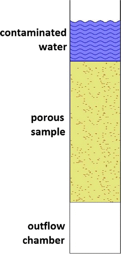
We propose a method to obtain an acceptable approximation of the sorption isotherm. Let us have a vertically positioned sample of a homogeneous porous media. Above the sample, there is a contaminated liquid that infiltrates the sample. Below the sample, we have an initially empty outflow chamber, where the expelled liquid will be gathered (see Figure 1).

Figure 1. Sketch of the initial state of the experiment.

During the experiment, we refill the tube of the contaminated liquid at certain time points. We measure the outflow contaminant flux during the whole experiment; this is the only measurement used to determine the sorption isotherm.

There are some advantages of using a form free parametrization compared to modelling using a priori chosen isotherm. Obviously, the form free modelling is universal and therefore it can fit the measurements better. When we consider the solution of the inverse problem for different priori chosen isotherms, we can observe that the computation time usually grows significantly with the number of free parameters in the model. This is, however, not the case for the free form optimization projected to the M-dimensional space using localized splines. Here, when we increase M, the computational time remains almost identical, which allows us to use big value M. It is the advantage of using Gateaux differential, which computes all derivatives at once. We note that once we find the sorption isotherm using free form modelling, we can expect that it will be valid also for other input data.

In Section 2, we present a mathematical model of the coupled system. The numerical approximation of PDEs for transport, dispersion and adsorption leads to a corresponding system of ODEs, which is described in Section 3. In Section 4, we define the inverse problem and discuss our strategy for its solution. We introduce the numerical modelling of the dual system in Section 5. In Section 6, we describe in detail the finite-dimensional approximation mentioned before in Section 4. In Section 7, we present and discuss some numerical experiments.

2. Mathematical model

2.1. Equations of flow

We assume that the contaminant, the porous medium and the liquid have such properties that the flow of the liquid does not depend on the contaminant concentration and adsorption. The flow in porous media is modelled by Richards equation (see [9]), which in 1D has the form(1) $$\begin{array}{c}\hfill {\mathit{\partial }}_t\mathit{\theta }=-{\mathit{\partial }}_{x}q,x\in 〈0,d〉.\end{array}$$(1)

Here, $\mathit{\theta }$ denotes the saturation, $q$ denotes the liquid flux and $d$ is the length of the sample. The flux of the liquid is governed by(2) $$\begin{array}{c}\hfill q=-K_{s}k(\mathit{\theta })({\mathit{\partial }}_{x}h-1),\end{array}$$(2)

where $K_s$ is the saturated hydraulic conductivity, $h(x,t)$ is the pressure head and $k(\mathit{\theta })$ is the permeability-saturation function. We have used van Genuchten–Mualem model to parametrize functions $\mathit{\theta }(h)$ and $k(\mathit{\theta })$ (see [10]). If the top liquid reservoir is not empty, we assume that(3) $$\begin{array}{cc}\hfill {\mathit{\partial }}_{t}l(t)& =-q(0,t),\hfill \end{array}$$(3) (4) $$\begin{array}{cc}\hfill h(0,t)& =l(t),\hfill \end{array}$$(4)

where $l(t)$ denotes the amount of the liquid in the top liquid reservoir.

Otherwise, if the reservoir is empty, we have the no-flux boundary. At the bottom of the sample, the Neumann boundary condition is taken. We assume experiments with initially dry porous media, therefore we have regularized initial condition(5) $$\begin{array}{c}\hfill h(x,0)=-K,K>>0,x>0.\end{array}$$(5)

When we refill the top liquid reservoir to $l_i$ cm of the liquid at a certain time $t_i$, we simply change the pressure head at the boundary to the following value:(6) $$\begin{array}{c}\hfill h(0,t_i)=l_i.\end{array}$$(6)

2.2. Equations of the contaminant concentration and the adsorption

The mass-balance equation for contaminant concentration in the water is(7) $$\begin{array}{c}\hfill {\mathit{\partial }}_t(\mathit{\theta }w)+\mathit{\rho }{\mathit{\partial }}_{t}S+{\mathit{\partial }}_{x}f=0,\end{array}$$(7)

where product $\mathit{\theta }(x,t)w(x,t)$ is the mass of contaminant dissolved in the water per unit volume of porous media, $S(x,t)$ is the mass of contaminant adsorbed in the porous media per unit mass of porous media, $f(x,t)$ is the contaminant flux and $\mathit{\rho }$ is bulk density of the solid matrix of the porous medium. The contaminant flux is the superposition of advection and diffusion. As for the advection part, the corresponding contaminant flux is given by the expression(8) $$\begin{array}{c}\hfill f_{\mathrm{adv}}(x,t)=qw,\end{array}$$(8)

where $w(x,t)$ is the contaminant concentration in the liquid. The diffusion–dispersion part of the contaminant flux is, assuming isotropy of the porous medium, given by the expression(9) $$\begin{array}{c}\hfill f_{\mathrm{dis}}(x,t)=-(D_0\mathit{\theta }+{\mathit{\alpha }}_{L}q){\mathit{\partial }}_{x}w,\end{array}$$(9)

where $D_0$ is the molecular diffusion constant and ${\mathit{\alpha }}_L$ is the longitudinal dispersion. The total flux is the sum of the advection flux and the diffusion–dispersion flux, and is therefore given by the equation(10) $$\begin{array}{c}\hfill f(x,t)=qw-(D_0\mathit{\theta }+{\mathit{\alpha }}_{L}q){\mathit{\partial }}_{x}w.\end{array}$$(10)

We will assume that the contaminant is present in the infiltrating water at maximal possible concentration and that at the bottom of the sample, the contaminant flux consists only of the advection part. Therefore, we have the following boundary conditions:(11) $$\begin{array}{cc}\hfill f(0,t)& =q(0,t),\hfill \end{array}$$(11) (12) $$\begin{array}{cc}\hfill {\mathit{\partial }}_{x}w(d,t)& =0.\hfill \end{array}$$(12)

We choose the non-equilibrium model with kinetics coefficient $\mathit{\kappa }$ to model the contaminant adsorption. The equation is(13) $$\begin{array}{c}\hfill {\mathit{\partial }}_{t}S=\mathit{\kappa }(\mathit{\psi }(w)-S),\end{array}$$(13)

where $\mathit{\psi }(w)$ is the sorption isotherm. We suppose that at the beginning of the experiment, the sample is contaminant free and therefore the initial conditions are(14) $$\begin{array}{c}\hfill S(x,0)=0,w(x,0)=0.\end{array}$$(14)

3. Numerical model

3.1. Numerical model of the flow

There are several numerical schemes available for numerical solution of the saturation, see e.g. [8] or [11]. We have used the same numerical model as in [8], specifically(15) $$\begin{array}{cc}& \frac{{\mathit{\theta }}_i^{j+1}-{\mathit{\theta }}_i^j}{\mathrm{\Delta }{t}^j}=\frac{q_{i-1/2}^{j+1}-q_{i+1/2}^{j+1}}{\mathrm{\Delta }x},i=1,2,\dots ,N-1,\hfill \end{array}$$(15) (16) $$\begin{array}{cc}& q_{i+1/2}=-K_s\frac{k({\mathit{\theta }}_i)+k({\mathit{\theta }}_{i+1})}{2}\left(\frac{h_{i+1}-h_i}{\mathrm{\Delta }x}-1\right),i=0,1,\dots ,N-1,\hfill \end{array}$$(16) (17) $$\begin{array}{c}\hfill \left\{\begin{array}{cccc}\frac{{\mathit{\theta }}_0^{j+1}-{\mathit{\theta }}_0^j}{\mathrm{\Delta }{t}^j}=-2\frac{q_{1/2}^{j+1}}{\mathrm{\Delta }x}\hfill & \text{and}& q_0=0,\hfill & \mathrm{if}{h}_0^j<=0\\ \frac{h_0^{j+1}-h_0^j}{\mathrm{\Delta }{t}^j}=-q_0\hfill & \mathrm{and}& q_0=-K_s\left(\frac{h_1-h_0}{\mathrm{\Delta }x}-1\right),\hfill & \mathrm{if}{h}_0^j>0\end{array}\right.,\end{array}$$(17) (18) $$\begin{array}{c}\hfill \frac{{\mathit{\theta }}_N^{j+1}-{\mathit{\theta }}_N^j}{\mathrm{\Delta }{t}^j}=2\frac{q_{N-1/2}^{j+1}-q_N^{j+1}}{\mathrm{\Delta }x},q_N=K_{s}k({\mathit{\theta }}_N).\end{array}$$(18)

The indices $i,j$ correspond to the space and time discretization, respectively.

3.2. Numerical model of the contaminant concentration and the adsorption

We use the mass-preserving finite volumes method to obtain the semidiscretization of our problem. After setting $x_i=d\frac{i}{N},i=0,1,\dots ,N,\mathrm{\Delta }x=d/N$, we obtain the semidiscretization of coupled system (7(7) $$\begin{array}{c}\hfill {\mathit{\partial }}_t(\mathit{\theta }w)+\mathit{\rho }{\mathit{\partial }}_{t}S+{\mathit{\partial }}_{x}f=0,\end{array}$$(7) ), (13(13) $$\begin{array}{c}\hfill {\mathit{\partial }}_{t}S=\mathit{\kappa }(\mathit{\psi }(w)-S),\end{array}$$(13) ) with boundary conditions (11(11) $$\begin{array}{cc}\hfill f(0,t)& =q(0,t),\hfill \end{array}$$(11) ), (12(12) $$\begin{array}{cc}\hfill {\mathit{\partial }}_{x}w(d,t)& =0.\hfill \end{array}$$(12) ):(19) $$\begin{array}{cc}\hfill {\mathit{\partial }}_t({\mathit{\theta }}_i{w}_i)& =\frac{1}{\mathrm{\Delta }x}(q_{i-1/2}{w}_{i-1/2}-(D_0{\mathit{\theta }}_{i-1/2}+{\mathit{\alpha }}_L{q}_{i-1/2})\frac{w_i-w_{i-1}}{\mathrm{\Delta }x}\hfill \\ \hfill & -q_{i+1/2}{w}_{i+1/2}+(D_0{\mathit{\theta }}_{i+1/2}+{\mathit{\alpha }}_L{q}_{i+1/2})\frac{w_{i+1}-w_i}{\mathrm{\Delta }x}-\mathit{\rho }\mathit{\kappa }(\mathit{\psi }(w_i)-S_i),\hfill \\ \hfill & i=1,\dots ,N-1,\hfill \end{array}$$(19) (20) $$\begin{array}{cc}\hfill {\mathit{\partial }}_t{S}_i& =\mathit{\kappa }(\mathit{\psi }(w_i)-S_i),i=0,1,\dots ,N,\hfill \end{array}$$(20) (21) $$\begin{array}{cc}\hfill {\mathit{\partial }}_t({\mathit{\theta }}_0{w}_0)& =\frac{2}{\mathrm{\Delta }x}(q_0-q_{1/2}{w}_{1/2}+(D_0{\mathit{\theta }}_{1/2}+{\mathit{\alpha }}_L{q}_{1/2})\frac{w_1-w_0}{\mathrm{\Delta }x}\hfill \\ \hfill & -\mathit{\rho }\mathit{\kappa }(\mathit{\psi }(w_0)-S_0),\hfill \end{array}$$(21) (22) $$\begin{array}{cc}\hfill {\mathit{\partial }}_t({\mathit{\theta }}_N{w}_N)& =\frac{2}{\mathrm{\Delta }x}(q_{N-1/2}{w}_{N-1/2}\hfill \\ \hfill & -(D_0{\mathit{\theta }}_{N-1/2}+{\mathit{\alpha }}_L{q}_{N-1/2})\frac{w_N-w_{N-1}}{\mathrm{\Delta }{x}_{N-1}}-q_N{w}_N)-\mathit{\rho }\mathit{\kappa }(\mathit{\psi }(w_N)-S_N).\hfill \end{array}$$(22)

This system of ODEs can be solved using MATLAB’s built-in ode15s solver. We note that $w_{i-1/2}=(w_{i-1}+w_i)/2$. Values ${\mathit{\theta }}_i$, $q_0$, $q_{i-1/2}$ and $q_N$ are available in discrete time points from simulation of flow and we have taken ${\mathit{\theta }}_{i-1/2}=({\mathit{\theta }}_{i-1}+{\mathit{\theta }}_i)/2$. We have extended the values of flux and saturation to any time point using cubic spline interpolation.

4. Inverse problem

In our proposed scenario, the outflow liquid flux together with its concentration are measured; therefore, we assume that we have a measurement $m(t)$ of the outflow contaminant flux. Further, we assume that the only unknown in the model is the sorption isotherm, which we want to determine. The main idea of our method is as follows: we construct the cost functional(23) $$\begin{array}{c}\hfill J(\mathit{\psi })={\int }_0^{T_f}{(q(d,t)w_{\mathit{\psi }}(d,t)-m(t))}^2\mathrm{d}t,\end{array}$$(23)

where $\mathit{\psi }\equiv \mathit{\psi }(w)$ is a sorption isotherm (dependent on contaminant concentration in the water $w\in 〈0,1〉$) used in our coupled system, $w_{\mathit{\psi }}(d,t)$ is the contaminant concentration at time $t$ at the sample outflow computed from our system using $\mathit{\psi }$ and $T_f$ is the time of the end of the experiment. We search for $\mathit{\psi }$ in the set of all functions satisfying the required qualitative properties, for which the functional value $J$ is minimal. These required properties are:(24) $$\begin{array}{c}\hfill \mathit{\psi }\in C^1(0,1),\mathit{\psi }\ge 0,\mathit{\psi }(0)=0,{\mathit{\psi }}^{\prime }\ge 0,\end{array}$$(24)

where $C^1(0,1)$ denotes the class of continuously differentiable functions. The main tool for finding the solution is to construct the differential of Gateaux,(25) $$\begin{array}{c}\hfill \mathit{\delta }J(\mathit{\psi },s)=\underset{\mathit{\epsilon }\to 0^{+}}{lim}\frac{J(\mathit{\psi }+\mathit{\epsilon }s)-J(\mathit{\psi })}{\mathit{\epsilon }}.\end{array}$$(25)

We then improve, in an iterative way, ${\mathit{\psi }}_n$ in the direction of $s_n$ ($n$ is the order of the iteration), where $\mathit{\delta }J({\mathit{\psi }}_n,s_n)<0$. Since we have constrains on the function ${\mathit{\psi }}_n$ and the current iteration ${\mathit{\psi }}_n$ can be on the boundary of the admissible set, we cannot use the direction of the steepest descent, as this may lead us outside the admissible region, no matter how small a step we take. We use the projected gradient method to overcome this problem.

The construction of the differential $\mathit{\delta }J(\mathit{\psi },s)$ follows Lagrange’s idea – the construction of the dual system for dual variables (also known as Lagrange multiplicators). We assume the unknown function $\mathit{\psi }$ in the form ${\mathit{\psi }}^M(x)={\sum }_{i=0}^M{\mathit{\psi }}_i{b}_i(x)$, where ${\mathit{\psi }}_i$ are scalar coefficients and $b_i(x)$ are $C^1$ smooth locally supported splines corresponding to a discretization of the interval $⟨0,1⟩$ localized to small subintervals of $⟨0,1⟩$. Thus, ${\mathit{\psi }}^M(x)$ represents finite-dimensional approximation of $\mathit{\psi }$; it is a good approximation for $M$ large enough. Our finite-dimensional optimization problem reads as(26) $$\begin{array}{c}\hfill \underset{{\{{\mathit{\psi }}_i\}}_{i=0}^M\in {\mathbb{R}}_{+}^{M+1}\cap \mathbb{U}}{min}J\left(\sum _{i=0}^M{\mathit{\psi }}_i{b}_i(x)\right),\end{array}$$(26)

where $\mathbb{U}$ is the subset in ${\mathbb{R}}_{+}^{M+1}$ for admissible ${\{{\mathit{\psi }}_i\}}_{i=0}^M$, so that qualitative properties for ${\mathit{\psi }}^M(x)$ are met. To solve the finite-dimensional problem (26(26) $$\begin{array}{c}\hfill \underset{{\{{\mathit{\psi }}_i\}}_{i=0}^M\in {\mathbb{R}}_{+}^{M+1}\cap \mathbb{U}}{min}J\left(\sum _{i=0}^M{\mathit{\psi }}_i{b}_i(x)\right),\end{array}$$(26) ) in an iterative way, we use the form of Gateaux differential (25(25) $$\begin{array}{c}\hfill \mathit{\delta }J(\mathit{\psi },s)=\underset{\mathit{\epsilon }\to 0^{+}}{lim}\frac{J(\mathit{\psi }+\mathit{\epsilon }s)-J(\mathit{\psi })}{\mathit{\epsilon }}.\end{array}$$(25) ), which gives us simultaneously all partial derivatives $\frac{\mathit{\partial }J({\mathit{\psi }}^M)}{\mathit{\partial }{\mathit{\psi }}_i}$. This procedure allows us to avoid the common numerical computation of $\frac{\mathit{\partial }J({\mathit{\psi }}^M)}{\mathit{\partial }{\mathit{\psi }}_i}$, which, for large M, would be very inefficient.

5. Computation of the variation in a direction $\mathit{\delta }\mathit{\psi }$

We use the following notation of variation along a given direction $\mathit{\delta }\mathit{\psi }$:(27) $$\begin{array}{c}\hfill \mathit{\delta }J=\underset{\mathit{\epsilon }\to 0^{+}}{lim}\frac{J(\mathit{\psi }+\mathit{\epsilon }\mathit{\delta }\mathit{\psi })-J(\mathit{\psi })}{\mathit{\epsilon }}.\end{array}$$(27)

Theorem 1

The variation of the function $J$ in the direction $\mathit{\delta }\mathit{\psi }$ has the following form:(28) $$\begin{array}{c}\hfill \mathit{\delta }J={\int }_0^{T_f}{\int }_0^d(\mathit{\delta }\mathit{\psi })(w)[\mathit{\kappa }(\mathit{\rho }\mathit{\lambda }-\mathit{\mu })]\mathrm{d}x\mathrm{d}t,\end{array}$$(28)

where $\mathit{\lambda }(x,t)$ and $\mathit{\mu }(x,t)$ are the adjoint functions (Lagrange multiplicators) to $w$ and $S$ defined by following ‘adjoint’ PDEs:(29) $$\begin{array}{cc}& \mathit{\theta }{\mathit{\partial }}_t\mathit{\lambda }+q{\mathit{\partial }}_x\mathit{\lambda }+{\mathit{\partial }}_x({\mathit{\partial }}_x\mathit{\lambda }(D_0\mathit{\theta }+{\mathit{\alpha }}_{L}q))-\mathit{\kappa }{\mathit{\psi }}^{\prime }(w)(\mathit{\lambda }\mathit{\rho }-\mathit{\mu })=0,\hfill \end{array}$$(29) (30) $$\begin{array}{cc}& {\mathit{\partial }}_t\mathit{\mu }=\mathit{\kappa }(\mathit{\mu }-\mathit{\rho }\mathit{\lambda }),\hfill \end{array}$$(30) (31) $$\begin{array}{cc}& {[q\mathit{\lambda }+(D_0\mathit{\theta }+{\mathit{\alpha }}_{L}q){\mathit{\partial }}_x\mathit{\lambda }+2(qw-m)q]}_{x=d}=0,\hfill \end{array}$$(31) (32) $$\begin{array}{cc}& {\mathit{\partial }}_x\mathit{\lambda }(0,t)=0,\hfill \end{array}$$(32) (33) $$\begin{array}{cc}& \mathit{\lambda }(x,T_f)=0,\mathit{\mu }(x,T_f)=0.\hfill \end{array}$$(33)

Proof

The proof follows the common Lagrange’s method (see [12]). For arbitrary functions $\mathit{\lambda },\mathit{\mu }$ we add the zero (see (7(7) $$\begin{array}{c}\hfill {\mathit{\partial }}_t(\mathit{\theta }w)+\mathit{\rho }{\mathit{\partial }}_{t}S+{\mathit{\partial }}_{x}f=0,\end{array}$$(7) ), (13(13) $$\begin{array}{c}\hfill {\mathit{\partial }}_{t}S=\mathit{\kappa }(\mathit{\psi }(w)-S),\end{array}$$(13) ), (10(10) $$\begin{array}{c}\hfill f(x,t)=qw-(D_0\mathit{\theta }+{\mathit{\alpha }}_{L}q){\mathit{\partial }}_{x}w.\end{array}$$(10) )) to the objective function $J$ and obtain the following equation:(34) $$\begin{array}{cc}\hfill J& ={\int }_0^{T_f}{(q(d,t)w(d,t)-m(t))}^2\mathrm{d}t+{\int }_0^{T_f}{\int }_0^d\left\{\mathit{\lambda }[{\mathit{\partial }}_t(\mathit{\theta }w)+{\mathit{\partial }}_x(qw\right.\hfill \\ \hfill & \left.-(D_0\mathit{\theta }+{\mathit{\alpha }}_{L}q){\mathit{\partial }}_{x}w)+\mathit{\rho }\mathit{\kappa }(\mathit{\psi }(w)-S)]+\mathit{\mu }[{\mathit{\partial }}_{t}S-\mathit{\kappa }(\mathit{\psi }(w)-S)]\right\}\mathrm{d}x\mathrm{d}t.\hfill \end{array}$$(34)

We note that we use various variations (e.g. $\mathit{\delta }w$, $\mathit{\delta }S$, etc.) along a direction $\mathit{\delta }\mathit{\psi }$ similarly to definition (27(27) $$\begin{array}{c}\hfill \mathit{\delta }J=\underset{\mathit{\epsilon }\to 0^{+}}{lim}\frac{J(\mathit{\psi }+\mathit{\epsilon }\mathit{\delta }\mathit{\psi })-J(\mathit{\psi })}{\mathit{\epsilon }}.\end{array}$$(27) ) as follows:(35) $$\begin{array}{c}\hfill \mathit{\delta }X(x,t)=\underset{\mathit{\epsilon }\to 0^{+}}{lim}\frac{X_{\mathit{\psi }+\mathit{\epsilon }\mathit{\delta }\mathit{\psi }}(x,t)-X_{\mathit{\psi }}(x,t)}{\mathit{\epsilon }},X\in \{w,S,\dots \}.\end{array}$$(35)

The variation $\mathit{\delta }J$ obtained from the Equation (34(34) $$\begin{array}{cc}\hfill J& ={\int }_0^{T_f}{(q(d,t)w(d,t)-m(t))}^2\mathrm{d}t+{\int }_0^{T_f}{\int }_0^d\left\{\mathit{\lambda }[{\mathit{\partial }}_t(\mathit{\theta }w)+{\mathit{\partial }}_x(qw\right.\hfill \\ \hfill & \left.-(D_0\mathit{\theta }+{\mathit{\alpha }}_{L}q){\mathit{\partial }}_{x}w)+\mathit{\rho }\mathit{\kappa }(\mathit{\psi }(w)-S)]+\mathit{\mu }[{\mathit{\partial }}_{t}S-\mathit{\kappa }(\mathit{\psi }(w)-S)]\right\}\mathrm{d}x\mathrm{d}t.\hfill \end{array}$$(34) ) has the following form:(36) $$\begin{array}{cc}\hfill \mathit{\delta }J& ={\int }_0^{T_f}2(q(d,t)w(d,t)-m(t))q(d,t)\mathit{\delta }w(d,t)\mathrm{d}t+{\int }_0^{T_f}{\int }_0^d\left\{\mathit{\lambda }[{\mathit{\partial }}_t(\mathit{\theta }\mathit{\delta }w)\right.\hfill \\ \hfill & +{\mathit{\partial }}_x(q\mathit{\delta }w-(D_0\mathit{\theta }+{\mathit{\alpha }}_{L}q){\mathit{\partial }}_x(\mathit{\delta }w))+\mathit{\rho }\mathit{\kappa }((\mathit{\delta }\mathit{\psi })(w)+{\mathit{\psi }}^{\prime }(w)\mathit{\delta }w-\mathit{\delta }S)]\hfill \\ \hfill & \left.+\mathit{\mu }[{\mathit{\partial }}_t(\mathit{\delta }S)-\mathit{\kappa }((\mathit{\delta }\mathit{\psi })(w)+{\mathit{\psi }}^{\prime }(w)\mathit{\delta }w-\mathit{\delta }S)]\right\}\mathrm{d}x\mathrm{d}t.\hfill \end{array}$$(36)

Using the integration by parts (to carry derivatives from $w$, $S$ to functions $\mathit{\lambda },\mathit{\mu }$), we get the following result:(37) $$\begin{array}{cc}\hfill \mathit{\delta }J& ={\int }_0^{T_f}{\int }_0^d\left\{\mathit{\delta }w[-\mathit{\theta }{\mathit{\partial }}_t\mathit{\lambda }-q{\mathit{\partial }}_x\mathit{\lambda }-{\mathit{\partial }}_x({\mathit{\partial }}_x\mathit{\lambda }(D_0\mathit{\theta }+{\mathit{\alpha }}_{L}q))\right.\hfill \\ \hfill & \left.+\mathit{\kappa }{\mathit{\psi }}^{\prime }(w)(\mathit{\lambda }\mathit{\rho }-\mathit{\mu })]+\mathit{\delta }S[-{\mathit{\partial }}_t\mathit{\mu }-\mathit{\rho }\mathit{\kappa }\mathit{\lambda }+\mathit{\kappa }\mathit{\mu }]+(\mathit{\delta }\mathit{\psi })(w)[\mathit{\kappa }(\mathit{\lambda }\mathit{\rho }-\mathit{\mu })]\right\}\mathrm{d}x\mathrm{d}t\hfill \\ \hfill & +{\int }_0^{T_f}\left\{\mathit{\delta }w(d,t){[2(qw-m)q+{\mathit{\partial }}_x\mathit{\lambda }(D_0\mathit{\theta }+{\mathit{\alpha }}_{L}q)+\mathit{\lambda }q]}_{x=d}\right.\hfill \\ \hfill & \left.+\mathit{\delta }({\mathit{\partial }}_{x}w(d,t)){[-\mathit{\lambda }(D_0\mathit{\theta }+{\mathit{\alpha }}_{L}q)]}_{x=d}\right\}-{\left[\mathit{\lambda }\mathit{\delta }\left(qw-(D_0\mathit{\theta }+{\mathit{\alpha }}_{L}q){\mathit{\partial }}_{x}w\right)\right]}_{x=0}\hfill \\ \hfill & -\mathit{\delta }w(0,t){\left[{\mathit{\partial }}_x\mathit{\lambda }(D_0\mathit{\theta }+{\mathit{\alpha }}_{L}q)\right]}_{x=0}\mathrm{d}t\hfill \\ \hfill & +{\int }_0^d\left[\mathit{\delta }w(x,T_f)\mathit{\lambda }(x,T_f)\mathit{\theta }(x,T_f)+\mathit{\delta }S(x,T_f)\mathit{\mu }(x,T_f)\right]\mathrm{d}x\hfill \end{array}$$(37)

We note that expressions $\mathit{\delta }({\mathit{\partial }}_{x}w(d,t))$ and $\mathit{\delta }{\left(qw-(D_0\mathit{\theta }+{\mathit{\alpha }}_{L}q){\mathit{\partial }}_{x}w\right)}_{x=0}$ equal zero, because of the boundary conditions (11(11) $$\begin{array}{cc}\hfill f(0,t)& =q(0,t),\hfill \end{array}$$(11) ), (12(12) $$\begin{array}{cc}\hfill {\mathit{\partial }}_{x}w(d,t)& =0.\hfill \end{array}$$(12) ). If we choose functions $\mathit{\lambda },\mathit{\mu }$ such that they are the solution of (29(29) $$\begin{array}{cc}& \mathit{\theta }{\mathit{\partial }}_t\mathit{\lambda }+q{\mathit{\partial }}_x\mathit{\lambda }+{\mathit{\partial }}_x({\mathit{\partial }}_x\mathit{\lambda }(D_0\mathit{\theta }+{\mathit{\alpha }}_{L}q))-\mathit{\kappa }{\mathit{\psi }}^{\prime }(w)(\mathit{\lambda }\mathit{\rho }-\mathit{\mu })=0,\hfill \end{array}$$(29) )–(33(33) $$\begin{array}{cc}& \mathit{\lambda }(x,T_f)=0,\mathit{\mu }(x,T_f)=0.\hfill \end{array}$$(33) ), we arrive at the form (28(28) $$\begin{array}{c}\hfill \mathit{\delta }J={\int }_0^{T_f}{\int }_0^d(\mathit{\delta }\mathit{\psi })(w)[\mathit{\kappa }(\mathit{\rho }\mathit{\lambda }-\mathit{\mu })]\mathrm{d}x\mathrm{d}t,\end{array}$$(28) ), thus completing the proof.

5.1. Semidiscretization of the adjoint equations

We can take advantage of the fact that we use the fixed semidiscretization to obtain the solution of the direct problem. We propose an analogous theorem to the Theorem 1, which will be formulated directly to the semidiscretization (19(19) $$\begin{array}{cc}\hfill {\mathit{\partial }}_t({\mathit{\theta }}_i{w}_i)& =\frac{1}{\mathrm{\Delta }x}(q_{i-1/2}{w}_{i-1/2}-(D_0{\mathit{\theta }}_{i-1/2}+{\mathit{\alpha }}_L{q}_{i-1/2})\frac{w_i-w_{i-1}}{\mathrm{\Delta }x}\hfill \\ \hfill & -q_{i+1/2}{w}_{i+1/2}+(D_0{\mathit{\theta }}_{i+1/2}+{\mathit{\alpha }}_L{q}_{i+1/2})\frac{w_{i+1}-w_i}{\mathrm{\Delta }x}-\mathit{\rho }\mathit{\kappa }(\mathit{\psi }(w_i)-S_i),\hfill \\ \hfill & i=1,\dots ,N-1,\hfill \end{array}$$(19) )–(22(22) $$\begin{array}{cc}\hfill {\mathit{\partial }}_t({\mathit{\theta }}_N{w}_N)& =\frac{2}{\mathrm{\Delta }x}(q_{N-1/2}{w}_{N-1/2}\hfill \\ \hfill & -(D_0{\mathit{\theta }}_{N-1/2}+{\mathit{\alpha }}_L{q}_{N-1/2})\frac{w_N-w_{N-1}}{\mathrm{\Delta }{x}_{N-1}}-q_N{w}_N)-\mathit{\rho }\mathit{\kappa }(\mathit{\psi }(w_N)-S_N).\hfill \end{array}$$(22) ). We apply spatially discrete adjoint functions to the semidiscretized adjoint problem. The resulting system of ODEs can be considered as the appropriate semidiscretization of ‘adjoint’ PDEs (29(29) $$\begin{array}{cc}& \mathit{\theta }{\mathit{\partial }}_t\mathit{\lambda }+q{\mathit{\partial }}_x\mathit{\lambda }+{\mathit{\partial }}_x({\mathit{\partial }}_x\mathit{\lambda }(D_0\mathit{\theta }+{\mathit{\alpha }}_{L}q))-\mathit{\kappa }{\mathit{\psi }}^{\prime }(w)(\mathit{\lambda }\mathit{\rho }-\mathit{\mu })=0,\hfill \end{array}$$(29) )–(33(33) $$\begin{array}{cc}& \mathit{\lambda }(x,T_f)=0,\mathit{\mu }(x,T_f)=0.\hfill \end{array}$$(33) ), resulting in the maximum possible accuracy. We note that here, the objective function $J$ is naturally modified – the term $q(d,t)w(d,t)$ is replaced by the $q_N(t)w_N(t)$.

Theorem 2

When we use the semidiscretization (19(19) $$\begin{array}{cc}\hfill {\mathit{\partial }}_t({\mathit{\theta }}_i{w}_i)& =\frac{1}{\mathrm{\Delta }x}(q_{i-1/2}{w}_{i-1/2}-(D_0{\mathit{\theta }}_{i-1/2}+{\mathit{\alpha }}_L{q}_{i-1/2})\frac{w_i-w_{i-1}}{\mathrm{\Delta }x}\hfill \\ \hfill & -q_{i+1/2}{w}_{i+1/2}+(D_0{\mathit{\theta }}_{i+1/2}+{\mathit{\alpha }}_L{q}_{i+1/2})\frac{w_{i+1}-w_i}{\mathrm{\Delta }x}-\mathit{\rho }\mathit{\kappa }(\mathit{\psi }(w_i)-S_i),\hfill \\ \hfill & i=1,\dots ,N-1,\hfill \end{array}$$(19) )–(22(22) $$\begin{array}{cc}\hfill {\mathit{\partial }}_t({\mathit{\theta }}_N{w}_N)& =\frac{2}{\mathrm{\Delta }x}(q_{N-1/2}{w}_{N-1/2}\hfill \\ \hfill & -(D_0{\mathit{\theta }}_{N-1/2}+{\mathit{\alpha }}_L{q}_{N-1/2})\frac{w_N-w_{N-1}}{\mathrm{\Delta }{x}_{N-1}}-q_N{w}_N)-\mathit{\rho }\mathit{\kappa }(\mathit{\psi }(w_N)-S_N).\hfill \end{array}$$(22) ), then the variation of the function $J$ in the direction $\mathit{\delta }\mathit{\psi }$ has the following form:(38) $$\begin{array}{cc}\hfill \mathit{\delta }J& ={\int }_0^{T_f}\frac{\mathrm{\Delta }x}{2}(\mathit{\delta }\mathit{\psi })(w_0)\mathit{\kappa }(\mathit{\rho }{\mathit{\lambda }}_0-{\mathit{\mu }}_0)+\mathrm{\Delta }x\left[\sum _{i=1}^{N-1}(\mathit{\delta }\mathit{\psi })(w_i)\mathit{\kappa }(\mathit{\rho }{\mathit{\lambda }}_i-{\mathit{\mu }}_i)\right]\hfill \\ \hfill & +\frac{\mathrm{\Delta }x}{2}(\mathit{\delta }\mathit{\psi })(w_N)\mathit{\kappa }(\mathit{\rho }{\mathit{\lambda }}_N-{\mathit{\mu }}_N)\mathrm{d}t,\hfill \end{array}$$(38)

where ${\mathit{\lambda }}_i(t)$ and ${\mathit{\mu }}_i(t)$ are adjoint functions (Lagrange multiplicators) to $w_i$ and $S_i$ defined by the following ‘adjoint’ system of ODEs:(39) $$\begin{array}{cc}\hfill {\mathit{\partial }}_t{\mathit{\lambda }}_0& =-\frac{1}{{\mathit{\theta }}_0}(q_{\frac{1}{2}}\frac{{\mathit{\lambda }}_1-{\mathit{\lambda }}_0}{\mathrm{\Delta }x}+2\frac{D_0{\mathit{\theta }}_{\frac{1}{2}}+{\mathit{\alpha }}_L{q}_{\frac{1}{2}}}{\mathrm{\Delta }x}\frac{{\mathit{\lambda }}_1-{\mathit{\lambda }}_0}{\mathrm{\Delta }x}-\mathit{\kappa }{\mathit{\psi }}^{\prime }(w_0)({\mathit{\lambda }}_0\mathit{\rho }-{\mathit{\mu }}_0)),\hfill \end{array}$$(39) (40) $$\begin{array}{cc}\hfill {\mathit{\partial }}_t{\mathit{\lambda }}_i& =-\frac{1}{{\mathit{\theta }}_i}(q_{i-\frac{1}{2}}\frac{{\mathit{\lambda }}_i-{\mathit{\lambda }}_{i-1}}{2\mathrm{\Delta }x}+q_{i+\frac{1}{2}}\frac{{\mathit{\lambda }}_{i+1}-{\mathit{\lambda }}_i}{2\mathrm{\Delta }x}\hfill \\ \hfill & +\frac{D_0{\mathit{\theta }}_{i+\frac{1}{2}}+{\mathit{\alpha }}_L{q}_{i+\frac{1}{2}}}{\mathrm{\Delta }x}\frac{{\mathit{\lambda }}_{i+1}-{\mathit{\lambda }}_i}{\mathrm{\Delta }x}-\frac{D_0{\mathit{\theta }}_{i-\frac{1}{2}}+{\mathit{\alpha }}_L{q}_{i-\frac{1}{2}}}{\mathrm{\Delta }x}\frac{{\mathit{\lambda }}_i-{\mathit{\lambda }}_{i-1}}{\mathrm{\Delta }x}\hfill \\ \hfill & -\mathit{\kappa }{\mathit{\psi }}^{\prime }(w_i)({\mathit{\lambda }}_i\mathit{\rho }-{\mathit{\mu }}_i)),i=1,2,\dots ,N-1,\hfill \end{array}$$(40) (41) $$\begin{array}{cc}\hfill {\mathit{\partial }}_t{\mathit{\lambda }}_N& =-\frac{1}{{\mathit{\theta }}_N}\left(q_{N-\frac{1}{2}}\frac{{\mathit{\lambda }}_N-{\mathit{\lambda }}_{N-1}}{\mathrm{\Delta }x}-2\frac{D_0{\mathit{\theta }}_{N-\frac{1}{2}}+{\mathit{\alpha }}_L{q}_{N-\frac{1}{2}}}{\mathrm{\Delta }x}\frac{{\mathit{\lambda }}_N-{\mathit{\lambda }}_{N-1}}{\mathrm{\Delta }x}\right.\hfill \\ \hfill & \left.-\frac{4(q_N{w}_N-m)q_N}{\mathrm{\Delta }x}-2q_N{\mathit{\lambda }}_N-\mathit{\kappa }{\mathit{\psi }}^{\prime }(w_N)({\mathit{\lambda }}_N\mathit{\rho }-{\mathit{\mu }}_N)\right),\hfill \end{array}$$(41) (42) $$\begin{array}{cc}\hfill {\mathit{\partial }}_t{\mathit{\mu }}_i& =\mathit{\kappa }({\mathit{\mu }}_i-\mathit{\rho }{\mathit{\lambda }}_i),i=0,1,\dots ,N,\hfill \end{array}$$(42) (43) $$\begin{array}{cc}\hfill {\mathit{\lambda }}_i(T_f)& =0,{\mathit{\mu }}_i(T_f)=0,i=0,1,\dots ,N.\hfill \end{array}$$(43)

Sketch of the proof

We use the Lagrange’s method again. For arbitrary functions ${\mathit{\lambda }}_i(t),{\mathit{\mu }}_i(t)(i=0,1,\dots ,N)$, we add the zero (see (19(19) $$\begin{array}{cc}\hfill {\mathit{\partial }}_t({\mathit{\theta }}_i{w}_i)& =\frac{1}{\mathrm{\Delta }x}(q_{i-1/2}{w}_{i-1/2}-(D_0{\mathit{\theta }}_{i-1/2}+{\mathit{\alpha }}_L{q}_{i-1/2})\frac{w_i-w_{i-1}}{\mathrm{\Delta }x}\hfill \\ \hfill & -q_{i+1/2}{w}_{i+1/2}+(D_0{\mathit{\theta }}_{i+1/2}+{\mathit{\alpha }}_L{q}_{i+1/2})\frac{w_{i+1}-w_i}{\mathrm{\Delta }x}-\mathit{\rho }\mathit{\kappa }(\mathit{\psi }(w_i)-S_i),\hfill \\ \hfill & i=1,\dots ,N-1,\hfill \end{array}$$(19) )–(22(22) $$\begin{array}{cc}\hfill {\mathit{\partial }}_t({\mathit{\theta }}_N{w}_N)& =\frac{2}{\mathrm{\Delta }x}(q_{N-1/2}{w}_{N-1/2}\hfill \\ \hfill & -(D_0{\mathit{\theta }}_{N-1/2}+{\mathit{\alpha }}_L{q}_{N-1/2})\frac{w_N-w_{N-1}}{\mathrm{\Delta }{x}_{N-1}}-q_N{w}_N)-\mathit{\rho }\mathit{\kappa }(\mathit{\psi }(w_N)-S_N).\hfill \end{array}$$(22) )) to the objective function $J$ and obtain the following equation:(44) $$\begin{array}{cc}\hfill J& ={\int }_0^{T_f}{(q_N(t)w_N(t)-m(t))}^2\mathrm{d}t+\mathrm{\Delta }x{\int }_0^{T_f}\{\frac{{\mathit{\lambda }}_0}{2}[{\mathit{\partial }}_t({\mathit{\theta }}_0{w}_0)-\frac{2}{\mathrm{\Delta }x}(q_0-q_{1/2}{w}_{1/2}\hfill \\ \hfill & +(D_0{\mathit{\theta }}_{1/2}+{\mathit{\alpha }}_L{q}_{1/2})\frac{w_1-w_0}{\mathrm{\Delta }x})+\mathit{\rho }\mathit{\kappa }(\mathit{\psi }(w_0)-S_0)]-\frac{{\mathit{\mu }}_0}{2}[{\mathit{\partial }}_t{S}_0-\mathit{\kappa }(\mathit{\psi }(w_0)-S_0)]\hfill \\ \hfill & +\{\sum _{i=1}^{N-1}{\mathit{\lambda }}_i[{\mathit{\partial }}_t({\mathit{\theta }}_i{w}_i)-\frac{1}{\mathrm{\Delta }x}(q_{i-1/2}{w}_{i-1/2}-(D_0{\mathit{\theta }}_{i-1/2}+{\mathit{\alpha }}_L{q}_{i-1/2})\frac{w_i-w_{i-1}}{\mathrm{\Delta }x}\hfill \\ \hfill & -q_{i+1/2}{w}_{i+1/2}-(D_0{\mathit{\theta }}_{i+1/2}+{\mathit{\alpha }}_L{q}_{i+1/2})\frac{w_{i+1}-w_i}{\mathrm{\Delta }x})+\mathit{\rho }\mathit{\kappa }(\mathit{\psi }(w_i)-S_i)]\hfill \\ \hfill & -{\mathit{\mu }}_i[{\mathit{\partial }}_t{S}_i-\mathit{\kappa }(\mathit{\psi }(w_i)-S_i)]\}+\frac{{\mathit{\lambda }}_N}{2}[{\mathit{\partial }}_t({\mathit{\theta }}_N{w}_N)-\frac{2}{\mathrm{\Delta }x}(q_{N-1/2}{w}_{N-1/2}\hfill \\ \hfill & -(D_0{\mathit{\theta }}_{N-1/2}+{\mathit{\alpha }}_L{q}_{N-1/2})\frac{w_N-w_{N-1}}{\mathrm{\Delta }x}-q_N{w}_N)+\mathit{\rho }\mathit{\kappa }(\mathit{\psi }(w_N)-S_N)]\hfill \\ \hfill & -\frac{{\mathit{\mu }}_N}{2}[{\mathit{\partial }}_t{S}_N-\mathit{\kappa }(\mathit{\psi }(w_N)-S_N)]\}\mathrm{d}t.\hfill \end{array}$$(44)

We again construct the variation $\mathit{\delta }J$ in (44(44) $$\begin{array}{cc}\hfill J& ={\int }_0^{T_f}{(q_N(t)w_N(t)-m(t))}^2\mathrm{d}t+\mathrm{\Delta }x{\int }_0^{T_f}\{\frac{{\mathit{\lambda }}_0}{2}[{\mathit{\partial }}_t({\mathit{\theta }}_0{w}_0)-\frac{2}{\mathrm{\Delta }x}(q_0-q_{1/2}{w}_{1/2}\hfill \\ \hfill & +(D_0{\mathit{\theta }}_{1/2}+{\mathit{\alpha }}_L{q}_{1/2})\frac{w_1-w_0}{\mathrm{\Delta }x})+\mathit{\rho }\mathit{\kappa }(\mathit{\psi }(w_0)-S_0)]-\frac{{\mathit{\mu }}_0}{2}[{\mathit{\partial }}_t{S}_0-\mathit{\kappa }(\mathit{\psi }(w_0)-S_0)]\hfill \\ \hfill & +\{\sum _{i=1}^{N-1}{\mathit{\lambda }}_i[{\mathit{\partial }}_t({\mathit{\theta }}_i{w}_i)-\frac{1}{\mathrm{\Delta }x}(q_{i-1/2}{w}_{i-1/2}-(D_0{\mathit{\theta }}_{i-1/2}+{\mathit{\alpha }}_L{q}_{i-1/2})\frac{w_i-w_{i-1}}{\mathrm{\Delta }x}\hfill \\ \hfill & -q_{i+1/2}{w}_{i+1/2}-(D_0{\mathit{\theta }}_{i+1/2}+{\mathit{\alpha }}_L{q}_{i+1/2})\frac{w_{i+1}-w_i}{\mathrm{\Delta }x})+\mathit{\rho }\mathit{\kappa }(\mathit{\psi }(w_i)-S_i)]\hfill \\ \hfill & -{\mathit{\mu }}_i[{\mathit{\partial }}_t{S}_i-\mathit{\kappa }(\mathit{\psi }(w_i)-S_i)]\}+\frac{{\mathit{\lambda }}_N}{2}[{\mathit{\partial }}_t({\mathit{\theta }}_N{w}_N)-\frac{2}{\mathrm{\Delta }x}(q_{N-1/2}{w}_{N-1/2}\hfill \\ \hfill & -(D_0{\mathit{\theta }}_{N-1/2}+{\mathit{\alpha }}_L{q}_{N-1/2})\frac{w_N-w_{N-1}}{\mathrm{\Delta }x}-q_N{w}_N)+\mathit{\rho }\mathit{\kappa }(\mathit{\psi }(w_N)-S_N)]\hfill \\ \hfill & -\frac{{\mathit{\mu }}_N}{2}[{\mathit{\partial }}_t{S}_N-\mathit{\kappa }(\mathit{\psi }(w_N)-S_N)]\}\mathrm{d}t.\hfill \end{array}$$(44) ), use the integration by parts (to carry time derivatives from $w$, $S$ to functions $\mathit{\lambda },\mathit{\mu }$) and rearrange the terms such that the terms ${\mathit{\lambda }}_i,{\mathit{\mu }}_i$ are standing before parenthesis. If we choose functions ${\mathit{\lambda }}_i,{\mathit{\mu }}_i$ such that they are solution to (39(39) $$\begin{array}{cc}\hfill {\mathit{\partial }}_t{\mathit{\lambda }}_0& =-\frac{1}{{\mathit{\theta }}_0}(q_{\frac{1}{2}}\frac{{\mathit{\lambda }}_1-{\mathit{\lambda }}_0}{\mathrm{\Delta }x}+2\frac{D_0{\mathit{\theta }}_{\frac{1}{2}}+{\mathit{\alpha }}_L{q}_{\frac{1}{2}}}{\mathrm{\Delta }x}\frac{{\mathit{\lambda }}_1-{\mathit{\lambda }}_0}{\mathrm{\Delta }x}-\mathit{\kappa }{\mathit{\psi }}^{\prime }(w_0)({\mathit{\lambda }}_0\mathit{\rho }-{\mathit{\mu }}_0)),\hfill \end{array}$$(39) )–(43(43) $$\begin{array}{cc}\hfill {\mathit{\lambda }}_i(T_f)& =0,{\mathit{\mu }}_i(T_f)=0,i=0,1,\dots ,N.\hfill \end{array}$$(43) ), we arrive at the form (38(38) $$\begin{array}{cc}\hfill \mathit{\delta }J& ={\int }_0^{T_f}\frac{\mathrm{\Delta }x}{2}(\mathit{\delta }\mathit{\psi })(w_0)\mathit{\kappa }(\mathit{\rho }{\mathit{\lambda }}_0-{\mathit{\mu }}_0)+\mathrm{\Delta }x\left[\sum _{i=1}^{N-1}(\mathit{\delta }\mathit{\psi })(w_i)\mathit{\kappa }(\mathit{\rho }{\mathit{\lambda }}_i-{\mathit{\mu }}_i)\right]\hfill \\ \hfill & +\frac{\mathrm{\Delta }x}{2}(\mathit{\delta }\mathit{\psi })(w_N)\mathit{\kappa }(\mathit{\rho }{\mathit{\lambda }}_N-{\mathit{\mu }}_N)\mathrm{d}t,\hfill \end{array}$$(38) ).

6. Projection to the finite-dimensional space

When we perform the actual iteration process on the computer, we have to project the infinite-dimensional function $\mathit{\psi }$ to some high-dimensional finite subspace. In our case, we use Bessel splines, which are $C^1$ class functions. We choose the formula with zero second derivatives at boundaries. Each Bessel spline is a linear combination of the basis functions $b_i$, and therefore we have:(45) $$\begin{array}{c}\hfill \mathit{\psi }(x)=\sum _{i=0}^M{\mathit{\psi }}_i{b}_i(x),\end{array}$$(45)

where ${\mathit{\psi }}_i$ are the parameters in the finite-dimensional approximation denoting the function value $\mathit{\psi }$ at point $x_i=\frac{i}{M}$.

The explicit formula for basis functions $b_i$ is(46) $$\begin{array}{cc}\hfill b_0(x)& =\left\{\begin{array}{cc}0,\hfill & \mathrm{for}x\notin ⟨x_0,x_2⟩\hfill \\ 1-\frac{5M}{4}(x-x_0)+\frac{M^3}{4}{(x-x_0)}^3,\hfill & \mathrm{for}x\in ⟨x_0,x_1⟩\hfill \\ -\frac{M}{2}(x-x_1)+M^2{(x-x_1)}^2-\frac{M^3}{2}{(x-x_1)}^3,\hfill & \mathrm{for}x\in ⟨x_1,x_2⟩\hfill \end{array}\right.,\hfill \\ \hfill b_1(x)& =\left\{\begin{array}{cc}0,\hfill & \mathrm{for}x\notin ⟨x_0,x_3⟩\hfill \\ \frac{3M}{2}(x-x_0)-\frac{M^3}{2}{(x-x_0)}^3,\hfill & \mathrm{for}x\in ⟨x_0,x_1⟩\hfill \\ 1-\frac{5M^2}{2}{(x-x_1)}^2+\frac{3M^3}{2}{(x-x_1)}^3,\hfill & \mathrm{for}x\in ⟨x_1,x_2⟩\hfill \\ -\frac{M}{2}(x-x_2)+M^2{(x-x_2)}^2-\frac{M^3}{2}{(x-x_2)}^3,\hfill & \mathrm{for}x\in ⟨x_2,x_3⟩\hfill \end{array}\right.,\hfill \\ \hfill b_i(x)& =\left\{\begin{array}{cc}0,\hfill & \mathrm{for}x\notin ⟨x_{i-2},x_{i+2}⟩\hfill \\ -\frac{M^2}{2}{(x-x_{i-2})}^2+\frac{M^3}{2}{(x-x_{i-2})}^3,\hfill & \mathrm{for}x\in ⟨x_{i-2},x_{i-1}⟩\hfill \\ \frac{M}{2}(x-x_{i-1})+2M^2{(x-x_{i-1})}^2-\frac{3M^3}{2}{(x-x_{i-1})}^3,\hfill & \mathrm{for}x\in ⟨x_{i-1},x_i⟩\hfill \\ 1-\frac{5M^2}{2}{(x-x_i)}^2+\frac{3M^3}{2}{(x-x_i)}^3,\hfill & \mathrm{for}x\in ⟨x_i,x_{i+1}⟩\hfill \\ -\frac{M}{2}(x-x_{i+1})+M^2{(x-x_{i+1})}^2-\frac{M^3}{2}{(x-x_{i+1})}^3,\hfill & \mathrm{for}x\in ⟨x_{i+1},x_{i+2}⟩\hfill \end{array}\right.,\hfill \\ \hfill b_{M-1}(x)& =\left\{\begin{array}{cc}0,\hfill & \mathrm{for}x\notin ⟨x_{M-3},x_M⟩\hfill \\ -\frac{M^2}{2}{(x-x_{M-3})}^2+\frac{M^3}{2}{(x-x_{M-3})}^3,\hfill & \mathrm{for}x\in ⟨x_{M-3},x_{M-2}⟩\hfill \\ \frac{M}{2}(x-x_{M-2})+2M^2{(x-x_{M-2})}^2-\frac{3M^3}{2}{(x-x_{M-2})}^3,\hfill & \mathrm{for}x\in ⟨x_{M-2},x_{M-1}⟩\hfill \\ 1-\frac{3M^2}{2}{(x-x_{M-1})}^2+\frac{M^3}{2}{(x-x_{M-1})}^3,\hfill & \mathrm{for}x\in ⟨x_{M-1},x_M⟩\hfill \end{array}\right.,\hfill \\ \hfill b_M(x)& =\left\{\begin{array}{cc}0,\hfill & \mathrm{for}x\notin ⟨x_{M-2},x_M⟩\hfill \\ -\frac{M^2}{2}{(x-x_{M-2})}^2+\frac{M^3}{2}{(x-x_{M-2})}^3,\hfill & \mathrm{for}x\in ⟨x_{M-2},x_{M-1}⟩\hfill \\ \frac{M}{2}(x-x_{M-1})+\frac{3M^2}{4}{(x-x_{M-1})}^2-\frac{M^3}{4}{(x-x_{M-1})}^3,\hfill & \mathrm{for}x\in ⟨x_{M-1},x_M⟩\hfill \end{array}\right.,\hfill \end{array}$$(46)

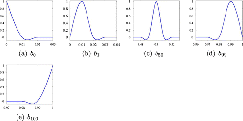
where $M+1$ is the number of Bessel splines used. In Figure 2, we show some of these basis functions for $M=100$:

Figure 2. Some basis functions of Bessel splines for $M=100$.

To write down the derivative of $J$ with respect to ${\mathit{\psi }}_i$, we simply use (45(45) $$\begin{array}{c}\hfill \mathit{\psi }(x)=\sum _{i=0}^M{\mathit{\psi }}_i{b}_i(x),\end{array}$$(45) ) and (38(38) $$\begin{array}{cc}\hfill \mathit{\delta }J& ={\int }_0^{T_f}\frac{\mathrm{\Delta }x}{2}(\mathit{\delta }\mathit{\psi })(w_0)\mathit{\kappa }(\mathit{\rho }{\mathit{\lambda }}_0-{\mathit{\mu }}_0)+\mathrm{\Delta }x\left[\sum _{i=1}^{N-1}(\mathit{\delta }\mathit{\psi })(w_i)\mathit{\kappa }(\mathit{\rho }{\mathit{\lambda }}_i-{\mathit{\mu }}_i)\right]\hfill \\ \hfill & +\frac{\mathrm{\Delta }x}{2}(\mathit{\delta }\mathit{\psi })(w_N)\mathit{\kappa }(\mathit{\rho }{\mathit{\lambda }}_N-{\mathit{\mu }}_N)\mathrm{d}t,\hfill \end{array}$$(38) ):(47) $$\begin{array}{cc}\hfill \frac{\mathit{\partial }J}{\mathit{\partial }{\mathit{\psi }}_j}& ={\int }_0^{T_f}\left[\frac{\mathrm{\Delta }x}{2}{b}_j(w_0)\mathit{\kappa }(\mathit{\rho }{\mathit{\lambda }}_0-{\mathit{\mu }}_0)+\mathrm{\Delta }x\sum _{i=1}^{N-1}{b}_j(w_i)\mathit{\kappa }(\mathit{\rho }{\mathit{\lambda }}_i-{\mathit{\mu }}_i)\right.\hfill \\ \hfill & \left.+\frac{\mathrm{\Delta }x}{2}{b}_j(w_N)\mathit{\kappa }(\mathit{\rho }{\mathit{\lambda }}_N-{\mathit{\mu }}_N)\right]\mathrm{d}t,j=0,1,\dots ,M.\hfill \end{array}$$(47)

We note that during the computation on the computer, we use the fact that our basis functions have finite support, and therefore we use it for fast computation of partial derivatives for all indices $i$. At the beginning of the computation, we set all partial derivatives to zero, we go through every element of our discretized spacetime and update only those derivatives corresponding to non-zero $b_j(w_i(t_k))$. We also note that exact compliance of conditions (24(24) $$\begin{array}{c}\hfill \mathit{\psi }\in C^1(0,1),\mathit{\psi }\ge 0,\mathit{\psi }(0)=0,{\mathit{\psi }}^{\prime }\ge 0,\end{array}$$(24) ) would be unnecessarily difficult to achieve. Therefore, we formulate similar, but not equivalent conditions for the values ${\mathit{\psi }}_i$:(48) $$\begin{array}{cc}& {\mathit{\psi }}_0=0;{\mathit{\psi }}_i\ge 0,i=1,\dots ,M;\hfill \\ \hfill & {\mathit{\psi }}_{i+1}-{\mathit{\psi }}_i\ge 0,i=0,\dots ,M-1.\hfill \end{array}$$(48)

We note, that these conditions are linear. Therefore, we can easily use projected gradient method to construct the new iteration. The formula for the new iteration is following:(49) $$\begin{array}{c}\hfill {\mathit{\psi }}^{k+1}=P({\mathit{\psi }}^k-\mathit{\alpha }\mathrm{\nabla }J({\mathit{\psi }}^k)),\end{array}$$(49)

where $P$ is projection operator to the admissible set given by (48(48) $$\begin{array}{cc}& {\mathit{\psi }}_0=0;{\mathit{\psi }}_i\ge 0,i=1,\dots ,M;\hfill \\ \hfill & {\mathit{\psi }}_{i+1}-{\mathit{\psi }}_i\ge 0,i=0,\dots ,M-1.\hfill \end{array}$$(48) ). The projection of the point $x$ ($x\leftrightarrow {\mathit{\psi }}^k-\mathit{\alpha }\mathrm{\nabla }J({\mathit{\psi }}^k)$) is given by the solution of the following quadratic programming problem:(50) $$\begin{array}{cc}& \underset{p}{min}{(p-x)}^T(p-x),\hfill \\ \hfill & p_i\ge 0,i=1,\dots ,M;\hfill \\ \hfill & p_{i+1}-p_i\ge 0,i=0,\dots ,M-1.\hfill \end{array}$$(50)

In each iteration, we perform an approximate line search to determine the step size. In this manner, we obtain a new iteration. We stop the iteration precess when the norm of difference between the two successive iterations is very small.

7. Results

First, let us focus on a simple experiment. Assume that we put the contaminated water on the top of the sample at the beginning of the experiment and we do not refill the injection chamber during infiltration. In this case, we are able to obtain in an iterative way such a function $\mathit{\psi }$ that the outflow contaminant flux corresponding to it is in agreement with the ‘measured’ flux. The two graphs of the ‘measured’ and the computed outflow contaminant flux are almost identical. 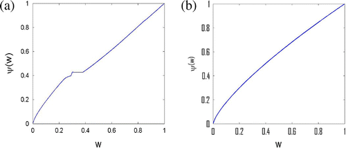However, the isotherm $\mathit{\psi }$ that was used to produce the ‘measured’ flux is significantly different from the one obtained by the iterative process (see Figure 3), which demonstrates the ill-posedness of our inverse problem. In Figure 3, we present two different isotherms $\mathit{\psi }$, which both produce an almost identical outflow contaminant flux:

Figure 3. Two different functions $\mathit{\psi }$ that in our scenario produced the equal outflow contaminant flux.

Therefore, we can observe that the data of the contaminant flux in the simple experiment proved to be insufficient to determine the sorption isotherm $\mathit{\psi }$ (or even a part of it). This is the reason why we simulate a more complex scenario, where the top liquid reservoir is refilled multiple times to stimulate the dynamics in the outflow contaminant flux (and force the solution of the direct problem to produce more values of the concentration $w$ in the sample). Let us assume the following common scenario in all remaining experiments. Let a 10 cm long porous medium sample be initially dry:(51) $$\begin{array}{c}\hfill u(x,0)=0,x>0.\end{array}$$(51)

Next, let there be a column of 3 cm of the contaminated liquid in the top liquid reservoir chamber at the beginning of the experiment. At the following time points $t_i$, we refill the chamber with 2 cm of contaminated liquid:(52) $$\begin{array}{c}\hfill t_i=20,000i,i=1,2,3,4.\end{array}$$(52)

We stop the simulation at time $T_f=200,000$. Let soil parameters be known and have following values:(53) $$\begin{array}{c}\hfill K_s=2.4\times {10}^{-4};n=2.81;\mathit{\alpha }=-0.0189;{\mathit{\theta }}_s=0.4;{\mathit{\theta }}_r=0.02.\end{array}$$(53)

Further, let contaminant and sorption parameters be as follows:(54) $$\begin{array}{c}\hfill D_0=5\times {10}^{-4};\mathit{\rho }=0.6;{\mathit{\alpha }}_L=1;\mathit{\kappa }={10}^{-3}.\end{array}$$(54)

Finally, let the initial contaminant/adsorption condition be as follows:(55) $$\begin{array}{c}\hfill w(x,0)=0;S(x,0)=0.\end{array}$$(55)

Now, the following experiments will differ only in the desired outflow contaminant flux $m$.

7.1. Experiment 1

In the first experiment, we produce $m$ by running the simulation with the Freundlich isotherm(56) $$\begin{array}{c}\hfill \mathit{\psi }(w)=w^{0,75},\end{array}$$(56)

and setting $m(t)=q(d,t)w(d,t)$. In the Figure 4, we present the final iteration ${\mathit{\psi }}_{165}$ of the algorithm together with the original Freundlich isotherm and the starting iteration ${\mathit{\psi }}_0(w)=w$.

Figure 4. Red (dot): initial linear iteration ${\mathit{\psi }}_0$; black (dash-dot): Freundlich isotherm (56(56) $$\begin{array}{c}\hfill \mathit{\psi }(w)=w^{0,75},\end{array}$$(56) ); blue (solid): final iteration ${\mathit{\psi }}_{165}$.

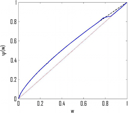
As we can see, the result is satisfactory within the interval $⟨0;0.8⟩$. In the neighbourhood of $1$, the result is flawed due to the fact that the values of the concentration greater than $0.8$ were rarely present during the experiment.

7.2. Experiment 2

In the second experiment, we obtain $m$ by performing the simulation with the following Langmuir isotherm:(57) $$\begin{array}{c}\hfill \mathit{\psi }(w)=\frac{2w}{w+1}.\end{array}$$(57)

In Figure 5, we present the final iteration ${\mathit{\psi }}_{270}$ of the algorithm together with the original Langmuir isotherm and the starting iteration ${\mathit{\psi }}_0(w)=w$.

Figure 5. Red (dot): initial linear iteration ${\mathit{\psi }}_0$; black (dash): Langmuir isotherm (57(57) $$\begin{array}{c}\hfill \mathit{\psi }(w)=\frac{2w}{w+1}.\end{array}$$(57) ); blue (solid): final iteration ${\mathit{\psi }}_{270}$.

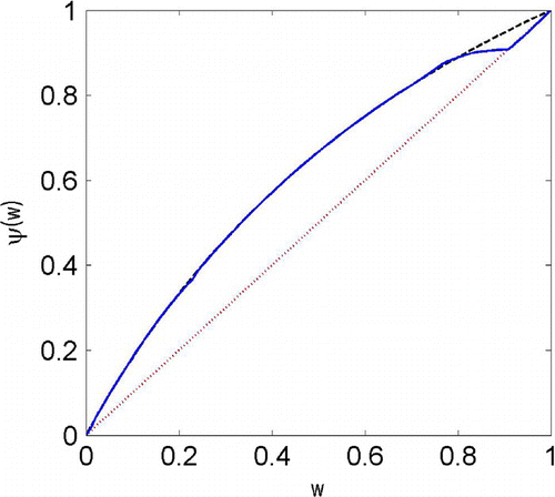
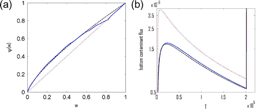
Figure 6. (a) Red (dot): initial linear iteration ${\mathit{\psi }}_0$; black (dash): Freundlich isotherm (56(56) $$\begin{array}{c}\hfill \mathit{\psi }(w)=w^{0,75},\end{array}$$(56) ); blue (solid): final iteration ${\mathit{\psi }}_{177}$. (b) Red (dot): $q(d,t)w(d,t)$ corresponding to ${\mathit{\psi }}_0$; black (dash): $q(d,t)w(d,t)$ corresponding to Freundlich isotherm (56(56) $$\begin{array}{c}\hfill \mathit{\psi }(w)=w^{0,75},\end{array}$$(56) ); blue (solid): both $q(d,t)w(d,t)$ corresponding to final iteration ${\mathit{\psi }}_{177}$ and $\tilde{m}$ obtained by running simulation using Freundlich isotherm (56(56) $$\begin{array}{c}\hfill \mathit{\psi }(w)=w^{0,75},\end{array}$$(56) ) and subsequently altered by the perturbation (58(58) $$\begin{array}{c}\hfill \tilde{m}=m(1+c_{1}sin(ln(t+1))+c_{2}cos(ln(t+1))).\end{array}$$(58) ).

Again, the result is satisfactory within the interval $⟨0;0.8⟩$. The reason for this observation is identical to the one mentioned in the previous experiment.

7.3. Experiment 3

In the third experiment, we determine $m$ by running the simulation with the same Freundlich isotherm as in Experiment 1, and then we apply the continuous (up to 5%) perturbation to the $m$ in the following form:(58) $$\begin{array}{c}\hfill \tilde{m}=m(1+c_{1}sin(ln(t+1))+c_{2}cos(ln(t+1))).\end{array}$$(58)

In the Figure 6, we present the final iteration ${\mathit{\psi }}_{177}$ of the algorithm together with the original Freundlich isotherm and the starting iteration ${\mathit{\psi }}_0(w)=w$. Additionally, we present the figure of the original measurement $m$ together with the altered $\tilde{m}$.

7.4. Experiment 4

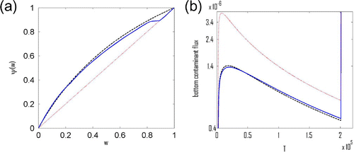
In the fourth experiment, we arrive at $m$ by performing the simulation with the same Langmuir isotherm as in Experiment 2, and then we apply the continuous perturbation to the $m$ as given by (58(58) $$\begin{array}{c}\hfill \tilde{m}=m(1+c_{1}sin(ln(t+1))+c_{2}cos(ln(t+1))).\end{array}$$(58) ). In Figure 7, we present the final iteration ${\mathit{\psi }}_{319}$ of the algorithm together with the original Langmuir isotherm and the starting iteration ${\mathit{\psi }}_0(w)=w$. Additionally, we present the figure of original measurement $m$ together with the altered $\tilde{m}$.

Figure 7. (a) Red (dot): initial linear iteration ${\mathit{\psi }}_0$; black(dash): Langmuir isotherm (57(57) $$\begin{array}{c}\hfill \mathit{\psi }(w)=\frac{2w}{w+1}.\end{array}$$(57) ); blue (solid): final iteration ${\mathit{\psi }}_{319}$. (b) Red (dot): $q(d,t)w(d,t)$ corresponding to ${\mathit{\psi }}_0$; black (dash): $q(d,t)w(d,t)$ corresponding to Langmuir isotherm (57(57) $$\begin{array}{c}\hfill \mathit{\psi }(w)=\frac{2w}{w+1}.\end{array}$$(57) ); blue (solid): both $q(d,t)w(d,t)$ corresponding to final iteration ${\mathit{\psi }}_{319}$ and $\tilde{m}$ obtained by running simulation using Langmuir isotherm (57(57) $$\begin{array}{c}\hfill \mathit{\psi }(w)=\frac{2w}{w+1}.\end{array}$$(57) ) and subsequently altered by the perturbation (58(58) $$\begin{array}{c}\hfill \tilde{m}=m(1+c_{1}sin(ln(t+1))+c_{2}cos(ln(t+1))).\end{array}$$(58) ).

7.5. Experiment 5

In the final experiment, we obtain $m$ by running the simulation with the same Freundlich isotherm as in Experiment 1, and then consider a random perturbation $\tilde{m}$ of $m$ obtained by multiplying $m$ with a random variate which is uniformly distributed in the interval $(0.95,1.05)$ at each time point for which the function has been enumerated. In Figure 8, we present the final iteration ${\mathit{\psi }}_{96}$ of the algorithm together with the original Freundlich isotherm and the starting iteration ${\mathit{\psi }}_0(w)=w$. Additionally, we present the figure of original measurement $m$ together with the altered $\tilde{m}$.

Figure 8. (a) Red (dot): initial linear iteration ${\mathit{\psi }}_0$; black (dash): Freundlich isotherm (56(56) $$\begin{array}{c}\hfill \mathit{\psi }(w)=w^{0,75},\end{array}$$(56) ); blue (solid): final iteration ${\mathit{\psi }}_{96}$. (b) Red (dot): $q(d,t)w(d,t)$ corresponding to ${\mathit{\psi }}_0$; black (dash): $q(d,t)w(d,t)$ corresponding to Freundlich isotherm (56(56) $$\begin{array}{c}\hfill \mathit{\psi }(w)=w^{0,75},\end{array}$$(56) ); blue (solid): $q(d,t)w(d,t)$ corresponding to final iteration ${\mathit{\psi }}_{96}$; green (dash-dot): $\tilde{m}$ obtained by running simulation using Freundlich isotherm (56(56) $$\begin{array}{c}\hfill \mathit{\psi }(w)=w^{0,75},\end{array}$$(56) ) and subsequently altered by the random noise.

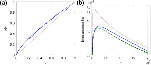
As we can see, results here are poor if compared to previous results. It is clear that some smoothing of the function $\tilde{m}$ is required prior to running the algorithm to determine $\mathit{\psi }$. This is to be expected, since, in the ‘adjoint’ differential equations, we assume $m$ to be a continuous function. This is however not valid in the case of Experiment 5, thus significantly decreasing the effectiveness of the proposed method to determine $\mathit{\psi }$.

8. Conclusions

We have proposed an effective experimental scenario to determine the sorption isotherm using non-invasive measurements of the outflow contaminant flux. We have not assumed that sorption isotherm is a member of some finite-dimensional class. Instead, we have performed a free form parametrization, where only some qualitative properties were assumed. We have stimulated the dynamics of the contaminant concentration at the outflow to increase the definiteness of the sorption isotherm. We have achieved the stimulation by multiple refilling of the injection chamber with contaminated water.

The main mathematical tool that we have used is the Gateaux differential. Once we have projected sorption isotherm into finite-dimensional space generated by localized splines, Gateaux differential enabled us to compute all partial derivatives without significant computational time penalty. Hence, we could choose large number of basis spline functions. Our numerical experiments with perturbation showed that our numerical method can reconstruct the sorption isotherm also in the cases, when measurements are affected by some error. We have obtained good results when the error was systematic (see Experiment 3 and 4) and flawed result when the error was stochastic and no a priori smoothing was used (see Experiment 5). This observation indicates that the sorption isotherm obtained using our method could be used for solution of the direct problem with the same sample and different initial and/or boundary conditions. Based on these facts, we think that proposed numerical procedure is a good candidate for the solution of the inverse problems.

Acknowledgements

The author thanks prof. Jozef Kačur for valuable discussions.

Additional information

Funding

The author confirms the financial support of the Slovak Research and Development Agency under the contracts [APVV-0184-10], [APVV-0743-10].

References

- Kačur J, Malengier B, Troj\’{a}kov\’{a} E. Numerical modelling of convection-diffusion-adsorption problems in 1D using dynamical discretization. Chem. Eng. Sci. 2010;65:2301–2309.
- Kr\"{a}utle S, Knabner P. A new numerical reduction scheme for fully coupled multicomponent transport-reaction problems in porous media. Water Resour. Res. 2005;41:1–17.
- Šim\‘{u}nek J, Nimo JR. Estimating soil hydraulic parameters from transient flow experiments in a centrifuge using parameter optimization technique. Water Resour. Res. 2005;41:1–9.
- Bitterlich S, Knabner P. An efficient method for solving an inverse problem for the Richards equation. J. Comput. Appl. Math. 2002;147:153–173.
- Ka\‘{e}ur J, Minár J. A benchmark solution for infiltration and adsorption of polluted water into unsaturated--saturated porous media. Transp. Porous Media. 2013;97:223–239.
- Thede G, Below E, Thede R. Determination of adsorption isotherms by the inverse method with a first order reversible reaction occurring in both phases of a liquid chromatographic column. J. Liq. Chromatogr. Related Technol. 2010;33:499–512.
- Huber JFK, Gerritse RG. Evaluation of dynamic gas chromatographic methods for the determination of adsorption and solution isotherms. J. Chromatogr. A. 1971;58:137–158.
- {\v{S}}imunek J, {\v{S}}ejna M, Saito H, Sakai M, van Genuchten MTh. The Hydrus-1D software package for simulating the movement of water, heat, and multiple solutes in variably saturated media. Version 4.0. HYDRUS Software Series 3, Riverside (CA): Department of Environmental Sciences/University of California Riverside; 2008.
- Bear J, Cheng H-D. Modeling groundwater flow and contaminant transport. New York (NY): Springer; 2010. ISBN-978-1402066818.
- van Genuchten MTh. A closed-form equation for predicting the hydraulic conductivity of unsaturated soils. Soil. Sci. Soc. Am. J. 1980;44:892–898.
- Troj{\’a}kov{\’a} E, Babušíková J. Contaminant transport in partially saturated porous media. In: Delgado JMPQ, de Lima AGB, da Silva MV, editors. Numerical analysis of heat and mass transfer in porous media. Vol. 27, Advanced structured materials. Berlin: Springer; 2012. p. 297–316. ISBN-978-3-642-30531-3.
- Bryson AE Jr, Ho Y-C. Applied optimal control. New York (NY): Hemisphere; 1975. ISBN-978-0891162285.