Modelling immune response to BK virus infection and donor kidney in renal transplant recipients

Abstract

In this paper, we develop and validate with bootstrapping techniques a mechanistic mathematical model of immune response to both BK virus infection and a donor kidney based on known and hypothesized mechanisms in the literature. The model presented does not capture all the details of the immune response but possesses key features that describe a very complex immunological process. We then estimate model parameters using a least squares approach with a typical set of available clinical data. Sensitivity analysis combined with asymptotic theory is used to determine the number of parameters that can be reliably estimated given the limited number of observations.

Keywords:

• renal transplant
• human polyomavirus type 1 (BKV)
• mathematical model
• inverse problem
• sensitivity analysis

AMS Subject Classifications:

• 62F12
• 65L09
• 92B05

1. Introduction

According to the OPTN/SRTR 2011 Annual Report, [1] 17,604 kidney transplants were performed in the United States between 2010 and 2011. Overall, there were 54,599 active candidates on the waiting list for kidney transplants, roughly threefold more than those that underwent transplant. These numbers reflect trends consistent with previous years, in which the number of patients waiting for transplants greatly exceeds the availability of organs. Given these facts, and the fact that as of 30 June 2011, 164,200 adults in the US were surviving with a functioning kidney graft, about twice as many as a decade earlier, optimal care of renal transplant patients is of great importance.

To reduce risk of allograft rejection, the standard of care for renal transplant recipients involves life-long pharmacological immunosuppression, making patients susceptible to opportunistic infections. Specifically, this therapy can render the recipients susceptible to an array of viral pathogens and may also reactivate latent viruses. For some time, human polyomavirus type 1, named ‘BK virus’ (BKV), has been a common pathogen found in kidney transplant patients. BKV is one of the two human polyomaviruses and was first discovered in 1970 in the urine of a kidney transplant patient with the initials BK.[2] This double-stranded non-enveloped DNA virus with icosahedral capsids asymptomatically infects more than 90% of the adult population worldwide and establishes a state of non-replicative infection,[3–5] or latent state. The infection is established in the kidneys and peripheral blood, specifically the renal tubular epithelial and urothelial cells, where replication-permissive cells express the viral capsid proteins followed by virion assembly in the nucleus.[6] This process eventually causes host cell lysis and the release of infectious progeny, deeming BKV replication as cytopathic, leading to a new round of active infection and latency. A high-level of BKV replication in the kidney results in a complication known as polyomavirus associated nephropathy (PVAN).[7–10] It is characterized by viral cytopathic changes of renal tubular epithelial cells, with enlarged nuclei, cell rounding, detachment and denudation of basal membranes.[11] Increasing prevalence rates of PVAN (1–10%) have been reported, with allograft dysfunction and loss in greater than 50% of cases.[12, 13] Therefore, PVAN is viewed as one of the leading causes of renal allograft loss in the first two years of transplantation. Unfortunately, there are no available licensed anti-polyoma viral drugs, and treatment relies on improving immune function to control BKV replication.[7] Given BKV infection is a significant health threat to immunosuppressed renal transplant patients, patient outcomes might be improved with the use of mathematical modelling to predict the course of the disease in individuals and recommend optimized treatment strategies.

Mathematical modelling is widely used and historically accepted in the physical science and engineering communities as an aid in the understanding of complex phenomena. Specifically, we highlight the use of mathematical modelling with experimental investigations to enhance the understanding of biological processes. The process involves a sequences of steps: (i) empirical observations, experiments and data collection; (ii) formalization of the biological model; (iii) abstraction of mathematical model; (iv) formalization of uncertainty and use of a statistical model; (v) model analysis; (vi) changes in understanding; and (vii) design of new experiments.[14] Given the highly iterative process of mathematical modelling and the recently developed quantitative techniques such as real-time PCR measurements of viral load, flow cytometry of T cell subsets and ELISPOT for virus-specifical T cell function, it is feasible to couple mathematical modelling with biological experimentation to investigate the dynamics of viral infection and the cellular immune response.

Here, we give a brief review of recent works that use mathematical modelling to investigate viral infection in relation to organ transplant dynamics. Funk et al. [9], summarized investigations of a retrospective analysis of BKV plasma load in renal transplant recipients undergoing allograft nephrectomy or changes in immunosuppressive regimens. PCR measurements of viral DNA are applied to a standard mathematical model for viral load decay kinetics to estimate the half-life and doubling time of BKV as well as clearance and growth rates.[9] This model addresses purely BKV replication. The next iteration in the modelling process requires the development of dynamic models that account for interactions between viral infection and host cell populations. Funk et al. [15] extended a one-compartment model to a two-compartment model with six state variables describing BKV replication dynamics in renal tubular epithelial cells and in urothelial cells. Estimation of parameters was based on population level clearance, proliferation, etc., rates. The study presented a basic model integrating two replication sites, the kidney and the urinary tract, and derived four variants which incorporated coupled and decoupled dynamics of the two sites. It remains unknown whether the two replicate sites are in fact coupled; however, results in Funk et al. [15] suggest that viral expansion was best explained by models where BKV replication started in the kidney followed by urothelial amplification and then reached an equilibrium amongst both replication sites. The model does not address the response of the immune system to viral infection and donor kidney and little to no statistically based model validation or calibration as proposed in our efforts here was carried out.

Other viral infections have been studied in relation to organ transplant dynamics. In particular, two models have been developed involving human cytomegalovirus (HCMV) infection. Kepler et al. [16] developed a dynamic model describing the pathogenesis of primary HCMV infection in immunocompetent and immunosuppressed patients at the cellular/viral mechanistic scale for application to individual clinical data and patient health. The model incorporates dynamics of the viral load, immune response as well as actively infected, susceptible and latently infected cells. Results highlight the necessity of longitudinal data for multiple state variables for robust parameter estimation. In addition, Banks et al. [17] developed a model to describe the immune response to both HCMV viral infection and introduction of a donor kidney in a renal transplant recipient. Dynamics of the viral load, susceptible and infected host cells, the immune response specific to viral infection and the transplant, and creatinine are incorporated into the model. Delineation between the cellular immune response to HCMV infection and the alloreactive immune response to the transplanted kidney as well as the incorporation of creatinine dynamics are vital additions to the dynamic model.

In the present effort, we develop a mathematical model of BKV infection and renal transplant dynamics at the cellular/viral mechanistic scale for application to renal transplant immunosuppressed individual clinical data. Specifically, we adapt dynamics of the HCMV model in Banks et al. [17] to allot for more specific BKV infection features. We eliminate the use of an antiviral treatment term, incorporate the effect of the alloreactive immune response and the presence of susceptible host cells on the clearance of creatinine, and add the effect of susceptible host cells on the concentration of allospecific CD8$+$ T cells. In contrast to the model in Funk et al. [15], we assume that the two BKV replication sites, the kidney and the urinary tract, are decoupled, focussing on the kidney as the main replication site. This choice was not only made given the inconclusive literature, but the data types available. Examining BKV replication within the urinary tract would require BKV urine data, which is not included in our available data-sets. We use a typically available data-set to pursue statistically based model validation or calibration in attempts to discern the specific information content one might expect in such a data-set.

The remainder of this paper is organized as follows. In Section 2, we present the biological model for which we base our mathematical model describing the immune response to both BKV infection and the introduction of a donor kidney in a renal transplant patient. An overview of clinical data acquired from collaborators is also given in Section 2. Model calibration and analysis is detailed in Section 3, where we give details regarding a log-transformed system, provide a detailed procedure for sensitivity analysis as well as outline our iterative inverse problem methodology. Details regarding computation of standard errors and confidence intervals are also discussed in Section 3. Results are given and discussed as well. In Section 4, we summarize efforts and conclusions drawn as well as suggest future research efforts.

2. Mathematical model description and data

In this section, we describe the dynamics of the viral load $V$, susceptible $H_S$ and infected $H_I$ host cells, BKV-specific $E_V$ and allospecific $E_K$ effector CD8$+$ T cells and serum creatinine $C$ with a brief description of the underlying biological model for which we base our mathematical model. Table 1 lists the state variables and Figure 1 diagrams the intracellular dynamics embodied in the model.

Table 1. Description of state variables.

State	Description	Units
$H_S$	Concentration of susceptible host cells	cells/mL
$H_I$	Concentration of infected host cells	cells/mL
$V$	Concentration of free BKV	copies/mL
$E_V$	Concentration of BKV-specific CD$8+$ T cells	cells/mL
$E_K$	Concentration of allospecific CD$8+$ T cells that target kidney	cells/mL
$C$	Concentration of serum creatinine	mg/dL

Figure 1. BKV model.

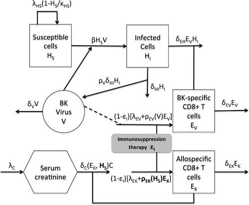
Active BKV infection targets both renal tubular epithelial cells and urothelial cells. For this model, however, we focus on one BKV target, the renal tubular epithelial cells. Susceptible host cells, the uninfected kidney tubular epithelial cells, $H_S$, in the absence of infection, are assumed to proliferate through the term ${\mathit{\lambda }}_{HS}\left(1-\frac{H_S}{{\mathit{\kappa }}_{HS}}\right)H_S$, indicating that new epithelial cells are derived from proliferation of existing $H_S$. Proliferation is modelled by logistic dynamics with ${\mathit{\lambda }}_{HS}$ being the maximum proliferation rate and ${\mathit{\kappa }}_{HS}$ is the cell density at which proliferation shuts off. A loss of susceptible cells, $H_S$, due to viral infection which occurs by cell-to-cell transmission, is represented by the term $\mathit{\beta }{H}_{S}V$. Here, we assume that one copy of virion infects one cell. Infected host cells or BKV replicating cells, $H_I$, lyse due to the cytopathic effect of BK virus, represented by the term ${\mathit{\delta }}_{HI}{H}_I$ and produce ${\mathit{\rho }}_V$ virions before death. In addition, infected host cells are eliminated by the BK-specific effector CD$8+$ T cells with rate term ${\mathit{\delta }}_{EH}{E}_V{H}_I$. Free virus is naturally cleared at the rate ${\mathit{\delta }}_V$ by the body and a loss of viral concentration is experienced through the infection of susceptible host cells.

The cellular immune response is the key defence against the BK viral infection. The terms ${\mathit{\lambda }}_{EV}$ and ${\mathit{\delta }}_{EV}$ represent the source and death rates of BK-specific effector CD$8+$ T cells. The concentration of BK-specific CD$8+$ T cells increases in response to the presence of free virus through the term ${\mathit{\rho }}_{EV}{E}_V$, where ${\mathit{\rho }}_{EV}$ is a bounded positive increasing function of free virus concentration. Specifically, ${\mathit{\rho }}_{EV}(V)=({\overline{\mathit{\rho }}}_{EV}V)/(V+{\mathit{\kappa }}_V)$ is a saturating nonlinearity with positive constants ${\overline{\mathit{\rho }}}_{EV}$ and ${\mathit{\kappa }}_V$. The alloreactive immune response to the transplanted kidney is incorporated into the model via a state variable, $E_K$, which denotes the effector CD$8+$ T cells that specifically target the transplant. The source rate for $E_K$, ${\mathit{\lambda }}_{EK}$, is dependent upon the HLA donor/recipient matching conducted prior to transplantation. Similar to the BK-specific CD$8+$ T cells, the concentration of allospecific CD$8+$ T cells increases in response to the presence of susceptible host cells $H_S$, since BK-virus targets kidney cells, represented by the term ${\mathit{\rho }}_{EK}{E}_K$, where ${\mathit{\rho }}_{EK}(H_S)=({\overline{\mathit{\rho }}}_{EK}{H}_S)/(H_S+{\mathit{\kappa }}_{KH})$ with positive constants ${\overline{\mathit{\rho }}}_{EV}$ and ${\mathit{\kappa }}_{KH}$. The death rate of $E_K$ is represented by ${\mathit{\delta }}_{EK}$.

Finally, we discuss the role of creatinine in the model. Creatinine is a waste product in the blood resulting from muscle activity and is removed by the healthy kidney. Therefore, serum creatinine concentration $C$ is used as a surrogate for glomerular filtration rate, a commonly used index of kidney function.[18] The production rate of $C$ is represented by ${\mathit{\lambda }}_C$ and when the kidney is impaired, creatinine is not effectively filtered and its concentration increases. To account for the negative effect of the alloreactive immune response $E_K$ on the kidney and the positive effect of susceptible cells $H_S$ (Recall that the renal allograft is a site of replication. Hence, the concentration of susceptible cells reflects the health of the kidney.), the clearance rate ${\mathit{\delta }}_C$ is defined as follows$${\mathit{\delta }}_C(E_K,H_S)=\frac{{\mathit{\delta }}_{C0}{\mathit{\kappa }}_{EK}}{E_K+{\mathit{\kappa }}_{EK}}·\frac{H_S}{H_S+{\mathit{\kappa }}_{CH}}.$$

Table 2 lists the parameters used in the model.

Table 2. Model parameters and their corresponding descriptions.

Parameter	Description	Unit
${\mathit{\lambda }}_{HS}$	Proliferation rate for $H_S$	1/day
${\mathit{\kappa }}_V$	Saturation constant	copies/mL
${\mathit{\kappa }}_{HS}$	Saturation constant	cells/mL
${\mathit{\lambda }}_{EK}$	Source rate of $E_K$	cells/(mL$·$day)
$\mathit{\beta }$	Infection rate of $H_S$ by $V$	mL/(copies$·$day)
${\mathit{\delta }}_{EK}$	Death rate of $E_K$	1/day
${\mathit{\delta }}_{HI}$	Death rate of $H_I$ by $V$	1/day
${\mathit{\lambda }}_C$	Production rate for $C$	mg/(dL$·$day)
${\mathit{\rho }}_V$	# Virions produced by $H_I$ before death	copies/cell
${\mathit{\delta }}_{C0}$	Maximum clearance rate for $C$	1/day
${\mathit{\delta }}_{EH}$	Elimination rate of $H_I$ by $E_V$	mL/(cells$·$day)
${\mathit{\kappa }}_{EK}$	Saturation constant	cells/mL
${\mathit{\delta }}_V$	Natural clearance rate of $V$	1/day
${\mathit{\kappa }}_{CH}$	Saturation constant	cells/mL
${\mathit{\lambda }}_{EV}$	Source rate of $E_V$	cells/(mL$·$day)
${\overline{\mathit{\rho }}}_{EK}$	Maximum proliferation rate for $E_K$	1/day
${\mathit{\delta }}_{EV}$	Death rate of $E_V$	1/day
${\mathit{\kappa }}_{KH}$	Saturation constant	cells/mL
${\overline{\mathit{\rho }}}_{EV}$	Maximum proliferation rate for $E_V$	1/day
${\mathit{\epsilon }}_I$	Efficacy of immunosuppressive drugs

Based on the above discussion, the model is given as follows:(1) $$\begin{array}{cc}\hfill \dot{H_S}& ={\mathit{\lambda }}_{HS}(1-\frac{H_S}{{\mathit{\kappa }}_{HS}})H_S-\mathit{\beta }{H}_{S}V,\hfill \end{array}$$(1) (2) $$\begin{array}{cc}\hfill \dot{H_I}& =\mathit{\beta }{H}_{S}V-{\mathit{\delta }}_{HI}{H}_I-{\mathit{\delta }}_{EH}{E}_V{H}_I,\hfill \end{array}$$(2) (3) $$\begin{array}{cc}\hfill \dot{V}& ={\mathit{\rho }}_V{\mathit{\delta }}_{HI}{H}_I-{\mathit{\delta }}_{V}V-\mathit{\beta }{H}_{S}V,\hfill \end{array}$$(3) (4) $$\begin{array}{cc}\hfill \dot{E_V}& =(1-{\mathit{ϵ}}_I)[{\mathit{\lambda }}_{EV}+{\mathit{\rho }}_{EV}(V)E_V]-{\mathit{\delta }}_{EV}{E}_V,\hfill \end{array}$$(4) (5) $$\begin{array}{cc}\hfill \dot{E_K}& =(1-{\mathit{ϵ}}_I)[{\mathit{\lambda }}_{EK}+{\mathit{\rho }}_{EK}(H_S)E_K]-{\mathit{\delta }}_{EK}{E}_K,\hfill \end{array}$$(5) (6) $$\begin{array}{cc}\hfill \dot{C}& ={\mathit{\lambda }}_C-{\mathit{\delta }}_C(E_K,H_S)C.\hfill \end{array}$$(6)

with initial conditions,(7) $$\begin{array}{c}\hfill (H_S(0),H_I(0),V(0),E_V(0),E_K(0),C(0))=(H_{S0},H_{I0},V_0,E_{V0},E_{K0},C_0).\end{array}$$(7)

We note that (1(1) $$\begin{array}{cc}\hfill \dot{H_S}& ={\mathit{\lambda }}_{HS}(1-\frac{H_S}{{\mathit{\kappa }}_{HS}})H_S-\mathit{\beta }{H}_{S}V,\hfill \end{array}$$(1) )–(4(4) $$\begin{array}{cc}\hfill \dot{E_V}& =(1-{\mathit{ϵ}}_I)[{\mathit{\lambda }}_{EV}+{\mathit{\rho }}_{EV}(V)E_V]-{\mathit{\delta }}_{EV}{E}_V,\hfill \end{array}$$(4) ) describe the immune response to the viral infection coupled with (5(5) $$\begin{array}{cc}\hfill \dot{E_K}& =(1-{\mathit{ϵ}}_I)[{\mathit{\lambda }}_{EK}+{\mathit{\rho }}_{EK}(H_S)E_K]-{\mathit{\delta }}_{EK}{E}_K,\hfill \end{array}$$(5) ) and (6(6) $$\begin{array}{cc}\hfill \dot{C}& ={\mathit{\lambda }}_C-{\mathit{\delta }}_C(E_K,H_S)C.\hfill \end{array}$$(6) ) describing the immune response to the transplanted kidney. Here, ${\mathit{\epsilon }}_I$ represents the efficacy of immunosuppressive drugs and is assumed to be scaled to less than or equal to $1$. This variable serves as the controller of the system to achieve balance between undersuppression and oversuppression of the patient’s immune system.

2.1. Data

The data for our investigation is from Massachusetts General Hospital and our discussions here consists of one patient record, TOS003. The data collection is performed as part of the patient’s routine medical care. Visits include pre-transplantation evaluation, day of transplant and post-transplantation visits. Day of transplant and post-transplantation visits are pertinent for model validation. Record TOS003 describes immunosuppression regimen, renal function recorded in plasma creatine (mg/dL) levels and infectious complications given in BKV viral plasma loads (in DNA copies/mL). TOS0003 associated data consists of eight viral load measurements and sixteen serum creatinine measurements. It should be noted that the recipient was diagnosed with ‘BK virus reactivation’ over the course of the first three months post-transplantation. It was documented that TOS003 was given immunosuppressive treatment upon organ transplantation and monitored accordingly. We note that the efficacy of the immunosuppression is a function of time, given the evidence in the data, however, it is difficult to quantify the efficacy of the immunosupression from the drug regimen records. The dosage, type and combination of drugs are changed after each visit. Hence, for simplicity, we assume that ${\mathit{\epsilon }}_I$ can be approximated by the following piecewise constant function.(8) $$\begin{array}{c}\hfill {\mathit{\epsilon }}_I(t)=\left\{\begin{array}{c}{\mathit{ϵ}}_1,t\in [0,21],\hfill \\ {\mathit{ϵ}}_2,t\in (21,60],\hfill \\ {\mathit{ϵ}}_3,t\in (60,120],\hfill \\ {\mathit{ϵ}}_4,t\in (120,450],\hfill \end{array}\right.\end{array}$$(8)

where the time frames are chosen based on the drug regimen record. It is also important to note that we are assuming test results displaying ‘None detected’ equate to the detection limit $20$ copies/mL of free virus in the system.[9] In addition, no test quantifying the BK viral load was conducted pre-transplant or the day of transplant; however, due to the seroprevalence of BKV in the population, it is assumed that the patient had a latent infection.

3. Model calibration and analysis

The model contains 6 variables and 29 constant parameters (model parameters and initial conditions). Equations (1(1) $$\begin{array}{cc}\hfill \dot{H_S}& ={\mathit{\lambda }}_{HS}(1-\frac{H_S}{{\mathit{\kappa }}_{HS}})H_S-\mathit{\beta }{H}_{S}V,\hfill \end{array}$$(1) )–(6(6) $$\begin{array}{cc}\hfill \dot{C}& ={\mathit{\lambda }}_C-{\mathit{\delta }}_C(E_K,H_S)C.\hfill \end{array}$$(6) ) were first written as a vector system$$\begin{array}{cc}& \dot{\overline{\mathbf{x}}}=\overline{\mathbf{g}}(\overline{\mathbf{x}};\overline{\mathbf{p}},{\overline{\mathbf{x}}}_0),\hfill \\ \hfill & \overline{\mathbf{x}}(0)={\overline{\mathbf{x}}}_0,\hfill \end{array}$$

where $\overline{\mathbf{x}}={[H_S,H_I,V,E_V,E_K,C]}^T$ is the vector of model states, $\overline{\mathbf{p}}=[{\mathit{\lambda }}_{HS},\mathit{\beta },{\mathit{\delta }}_{EH},{\mathit{\delta }}_V,{\overline{\mathit{\rho }}}_{EV},{\mathit{\delta }}_{EV},{\mathit{\delta }}_{EK},$${\mathit{\delta }}_{C0},{\mathit{\kappa }}_{HS},{\mathit{\delta }}_{HI},{\mathit{\rho }}_V,{\mathit{\lambda }}_{EV},$${\mathit{\kappa }}_V,{\mathit{\lambda }}_{EK},{\mathit{\lambda }}_C,{\mathit{\kappa }}_{EK},{\mathit{\kappa }}_{CH},{\overline{\mathit{\rho }}}_{EK},{\mathit{\kappa }}_{KH},{\mathit{ϵ}}_1,{\mathit{ϵ}}_2,{\mathit{ϵ}}_3,{\mathit{ϵ}}_4{]}^T\in {\mathbb{R}}^{23}$ is the vector of model parameters, and ${\overline{\mathbf{x}}}_0={[H_{S0},H_{I0},V_0,E_{V0},E_{K0},C_0]}^T\in {\mathbb{R}}^6$ is the set of initial conditions. Due to the scale difference between model states, we adopted the approach used in [19, 20]: solutions were determined for a log-transformed system. We remark that this is common in the biological literature to use log scale to deal with very large numbers; for example, in HIV studies and other viral infection studies both the viral load level (which can be as high as millions of copies/mL) and the changes in the viral load level can be large and hence they are often reported and analysed in log scale (e.g. see [21–23]). Since model parameter values and initial conditions are in different scales, a subset of the model parameters and initial conditions are also log-transformed to the log scale. This log-transformation approach is used to convert all the analysed quantities roughly to the same scale. It is worth noting that whenever we carry out a log-transformation for a quantity, we only log-transform its corresponding numerical value. In other words, ${log}_{10}(\overline{x})$ is always understood as a shorthand notation for ${log}_{10}((\overline{x}[\mathrm{units}])/(1[\mathrm{units}]))$ so the argument of log function is really dimensionless. An alternative approach, a common practice in engineering, to deal with the scale difference among analysed quantities is to normalize them so that the numerical values of the resulting quantities vary between 0 and 1, e.g. $x=(\overline{x}-{\overline{x}}_{\text{min}})/({\overline{x}}_{\text{max}}-{\overline{x}}_{\text{min}})$, where $x$ stands for quantity $\overline{x}$ after normalization and subscripts min and max, respectively, denote the minimal and maximal values of $\overline{x}$. However, for most biological applications, the minimal and maximal values of the analysed quantities are usually unknown and may vary among individuals, which is true for the problem we presented here. Thus, this normalization approach would result in a large number of extra unknown parameters that need to be identified (recall that the model contains 6 model states and 29 constant parameters). Considering the limited number of observations available to us, this approach can provide significant, if not impossible, challenges for the inverse problem investigated below and thus will not be considered in this paper.

Let,$$\begin{array}{cc}\hfill x_i& ={log}_{10}({\overline{x}}_i),i=1,2,3,4,5,\hfill \\ \hfill x_6& ={\overline{x}}_6,\hfill \\ \hfill x_{0i}& ={log}_{10}({\overline{x}}_{0i}),i=1,2,3,4,5,\hfill \\ \hfill x_{06}& ={\overline{x}}_{06},\hfill \\ \hfill p_j& ={log}_{10}({\overline{p}}_j),j=1,2,\cdots ,19,\hfill \\ \hfill p_j& ={\overline{p}}_j,j=20,21,22,23.\hfill \end{array}$$

Then we have the system(9) $$\begin{array}{cc}\hfill \dot{\mathbf{x}}& =\mathbf{g}(\mathbf{x};\mathbf{p},{\mathbf{x}}_{\mathbf{0}}),\mathbf{x}(\mathbf{0})={\mathbf{x}}_{\mathbf{0}},\hfill \end{array}$$(9)

where $\mathbf{g}={(g_1,g_2,\cdots g_6)}^T$ is given by$$\begin{array}{cc}\hfill g_i(\mathbf{x};\mathbf{p},{\mathbf{x}}_{\mathbf{0}})& =\frac{{10}^{-x_i}}{ln(10)}{\overline{g}}_i(\overline{\mathbf{x}};\overline{\mathbf{p}},{\overline{\mathbf{x}}}_0),i=1,2,\cdots 5,\hfill \\ \hfill g_6(\mathbf{x};\mathbf{p},{\mathbf{x}}_{\mathbf{0}})& ={\overline{g}}_6(\overline{\mathbf{x}};\overline{\mathbf{p}},{\overline{\mathbf{x}}}_0).\hfill \end{array}$$

We remark that by using the above log-transformed system (9(9) $$\begin{array}{cc}\hfill \dot{\mathbf{x}}& =\mathbf{g}(\mathbf{x};\mathbf{p},{\mathbf{x}}_{\mathbf{0}}),\mathbf{x}(\mathbf{0})={\mathbf{x}}_{\mathbf{0}},\hfill \end{array}$$(9) ), one can resolve a problem of states becoming unrealistically negative in solving model (1(1) $$\begin{array}{cc}\hfill \dot{H_S}& ={\mathit{\lambda }}_{HS}(1-\frac{H_S}{{\mathit{\kappa }}_{HS}})H_S-\mathit{\beta }{H}_{S}V,\hfill \end{array}$$(1) )–(6(6) $$\begin{array}{cc}\hfill \dot{C}& ={\mathit{\lambda }}_C-{\mathit{\delta }}_C(E_K,H_S)C.\hfill \end{array}$$(6) ) due to round-off error: nonnegative solutions of this model should stay so throughout numerical simulation. This log-transformation approach also enables the changes in model states due to the changes in parameters to be more measurable. In addition, this enables ready formulation of a reasonable stopping criterion for the inverse problem and can also make the associated optimization algorithm converge faster (vastly different magnitudes of analysed quantities increase condition numbers and hence the associated optimization algorithm may require more iterations to converge). From a statistical point of view, log-transformation is also a standard technique to render the observations more nearly normally distributed, and it is also commonly used to render heteroscedastic measurement errors more homoscedastic (e.g. see [24–26]) so that the resulting inverse problem is easier to implement (in ordinary least squares (OLS) approaches as opposed to generalized least squares approaches, e.g. see [26, 27] for details).

3.1. Forward simulations

Forward simulations were carried out by numerically solving the log-transformed version of model Equations (9(9) $$\begin{array}{cc}\hfill \dot{\mathbf{x}}& =\mathbf{g}(\mathbf{x};\mathbf{p},{\mathbf{x}}_{\mathbf{0}}),\mathbf{x}(\mathbf{0})={\mathbf{x}}_{\mathbf{0}},\hfill \end{array}$$(9) ) in Matlab using the ODE variable order variable step-size solver ode15s over a time course of 450 days. Parameter values used are listed in Table 3. The values of these parameters were either derived from published experimental studies or through simulation to acquire a benchmark value. For those parameters whose values can be found or derived from the literature, specifics are detailed below.

(1)	The parameter ${\mathit{\rho }}_V$, which quantifies the number of virions released by BKV-infected cells, was taken to be ${\mathit{\rho }}_{\mathbf{V}}\approx \mathbf{6000}$ copies/cell.[8, 9, 15, 28]
(2)	The measured BK viral half-life was found to be ${\mathbf{t}}_{\frac{\mathbf{1}}{\mathbf{2}}}\approx \mathbf{1.1}\mathbf{h}-\mathbf{9}\mathbf{days}$. This implies that the total clearance rate of BK is from $0.077$ to $15.1232$ per day. In the simulations, we set ${\mathit{\delta }}_V=0.4$ per day.[8, 15]

Table 3. Initial guess for parameter values $\mathit{\theta }=(\overline{\mathbf{p}},{\overline{\mathbf{x}}}_0)$ used in the parameter estimation simulations.

Parameter	Value	Parameter	Value
${\mathit{\lambda }}_{HS}$	0.03 per day	${\mathit{\kappa }}_{HS}$	$1\times {10}^3$ cells/mL
$\mathit{\beta }$	$8\times {10}^{-8}$ mL/(copies$·$day)	${\mathit{\delta }}_{HI}$	0.08 per day
${\mathit{\delta }}_{EH}$	$1.5\times {10}^{-3}$ mL/(cells$·$day)	${\mathit{\rho }}_V$	$6\times {10}^3$ copies/cell
${\mathit{\delta }}_V$	0.4 per day	${\mathit{\lambda }}_{EV}$	$1\times {10}^{-3}$ cells/(mL$·$day)
${\overline{\mathit{\rho }}}_{EV}$	0.3 per day	${\mathit{\kappa }}_V$	$100$ copies/mL
${\mathit{\delta }}_{EV}$	0.1 per day	${\mathit{\lambda }}_{EK}$	$2\times {10}^{-3}$ cells/(mL$·$day)
${\mathit{\delta }}_{EK}$	0.1 per day	${\mathit{\lambda }}_C$	$6\times {10}^{-3}$ mg/(dL$·$day)
${\mathit{\delta }}_{C0}$	0.01 per day	${\mathit{\kappa }}_{EK}$	0.2 cells/mL
${\mathit{\kappa }}_{CH}$	10 cells/mL	${\overline{\mathit{\rho }}}_{EK}$	0.2 per day
${\mathit{\kappa }}_{KH}$	85 cells/mL	${\mathit{ϵ}}_1$	0.1
${\mathit{ϵ}}_2$	0.38	${\mathit{ϵ}}_3$	0.6
${\mathit{ϵ}}_4$	0.3	$H_{S0}$	$5\times {10}^3$ cells/mL
$H_{I0}$	60 cells/mL	$V_0$	$5\times {10}^4$ copies/mL
$E_{V0}$	0.04 cells/mL	$E_{K0}$	0.4 cells/mL
$C_0$	1.07 mg/dL

3.2. Sensitivity analysis

In practice, one may be in a situation of estimating a large number of unknown parameters with a limited data-set. Such a situation is true in our case. To alleviate some of this difficulty, sensitivity analysis has been widely used in inverse problem investigations.[14, 20, 29–33] This process identifies the model parameters and initial conditions to which the model outputs are most sensitive. Specifically, sensitivity analysis provides insight into how changes in the parameters can affect the model output. In addition, this framework can be used to construct confidence intervals for parameter estimates using asymptotic properties of estimators.

To compute the sensitivities of model outputs to the model parameters and initial conditions, one proceeds to determine the sensitivity of each model state $x_i$ to each parameter $p_j$ and initial condition $x_{0j}$. These are defined as the derivatives of the model states with respect to the parameters, $\mathit{\partial }{x}_i/\mathit{\partial }{p}_j$ and $\mathit{\partial }{x}_i/\mathit{\partial }{x}_{0j}$, which satisfy in our case(10) $$\begin{array}{cc}& \frac{\mathrm{d}}{\mathrm{d}t}\frac{\mathit{\partial }{x}_i}{\mathit{\partial }{p}_j}=\sum _{l=1}^6\frac{\mathit{\partial }{g}_i}{\mathit{\partial }{x}_l}\frac{\mathit{\partial }{x}_l}{\mathit{\partial }{p}_j}+\frac{\mathit{\partial }{g}_i}{\mathit{\partial }{p}_j},\hfill \\ \hfill & \frac{\mathit{\partial }{x}_i}{\mathit{\partial }{p}_j}(0)=0,i=1,2,\cdots 6,j=1,2,\cdots ,23,\hfill \end{array}$$(10) (11) $$\begin{array}{cc}& \frac{\mathrm{d}}{\mathrm{d}t}\frac{\mathit{\partial }{x}_i}{\mathit{\partial }{x}_{0j}}=\sum _{l=1}^6\frac{\mathit{\partial }{g}_i}{\mathit{\partial }{x}_l}\frac{\mathit{\partial }{x}_l}{\mathit{\partial }{x}_{0j}},\hfill \\ \hfill & \frac{\mathit{\partial }{x}_i}{\mathit{\partial }{x}_{0j}}(0)={\mathit{\delta }}_{ij},i=1,2,\cdots 6,j=1,2,\cdots ,6,\hfill \end{array}$$(11)

where$$\begin{array}{c}\hfill {\mathit{\delta }}_{ij}=\left\{\begin{array}{c}1,i=j,\hfill \\ 0,i\ne j.\hfill \end{array}\right.\end{array}$$

The sensitivities $\frac{\mathit{\partial }\mathbf{x}}{\mathit{\partial }\mathbf{p}}$ and $\frac{\mathit{\partial }\mathbf{x}}{\mathit{\partial }{\mathbf{x}}_{\mathbf{0}}}$ can be calculated by solving (9(9) $$\begin{array}{cc}\hfill \dot{\mathbf{x}}& =\mathbf{g}(\mathbf{x};\mathbf{p},{\mathbf{x}}_{\mathbf{0}}),\mathbf{x}(\mathbf{0})={\mathbf{x}}_{\mathbf{0}},\hfill \end{array}$$(9) )–(11(11) $$\begin{array}{cc}& \frac{\mathrm{d}}{\mathrm{d}t}\frac{\mathit{\partial }{x}_i}{\mathit{\partial }{x}_{0j}}=\sum _{l=1}^6\frac{\mathit{\partial }{g}_i}{\mathit{\partial }{x}_l}\frac{\mathit{\partial }{x}_l}{\mathit{\partial }{x}_{0j}},\hfill \\ \hfill & \frac{\mathit{\partial }{x}_i}{\mathit{\partial }{x}_{0j}}(0)={\mathit{\delta }}_{ij},i=1,2,\cdots 6,j=1,2,\cdots ,6,\hfill \end{array}$$(11) ) simultaneously in Matlab using ode15s where the derivatives $\frac{\mathit{\partial }\mathbf{g}}{\mathit{\partial }\mathbf{x}}$, $\frac{\mathit{\partial }\mathbf{g}}{\mathit{\partial }\mathbf{p}}$ are obtained through automatic differentiation using myAD and tssolve in Matlab. In our case, we have data for both the free virus, $V$ and serum creatinine, $C$, states. Therefore, we only need to compute the sensitivities corresponding to states $x_i$, $i=3,6$. Initial conditions and model parameter values used are listed in Table 3. Results of the sensitivity analysis informed us as to which parameters were to be estimated. These findings along with the corresponding confidence intervals for these estimated parameters are described below.

It is worth emphasizing that sensitivity coefficients obtained above are for the log-transformed system (9(9) $$\begin{array}{cc}\hfill \dot{\mathbf{x}}& =\mathbf{g}(\mathbf{x};\mathbf{p},{\mathbf{x}}_{\mathbf{0}}),\mathbf{x}(\mathbf{0})={\mathbf{x}}_{\mathbf{0}},\hfill \end{array}$$(9) ). We note that in the case where $x_i={\overline{x}}_i$, $p_j={log}_{10}({\overline{p}}_j)$ and $x_{0j}={log}_{10}({\overline{x}}_{0j})$ we have,$$\begin{array}{c}\hfill \frac{\mathit{\partial }{x}_i}{\mathit{\partial }{p}_j}=\frac{\mathit{\partial }{x}_i}{\mathit{\partial }{\overline{x}}_i}\frac{\mathit{\partial }{\overline{x}}_i}{\mathit{\partial }{\overline{p}}_j}\frac{\mathit{\partial }{\overline{p}}_j}{\mathit{\partial }{p}_j}=log(10){\overline{p}}_j\frac{\mathit{\partial }{\overline{x}}_i}{\mathit{\partial }{\overline{p}}_j},\frac{\mathit{\partial }{x}_i}{\mathit{\partial }{x}_{0j}}=\frac{\mathit{\partial }{x}_i}{\mathit{\partial }{\overline{x}}_i}\frac{\mathit{\partial }{\overline{x}}_i}{\mathit{\partial }{\overline{x}}_{0j}}\frac{\mathit{\partial }{\overline{x}}_{0j}}{\mathit{\partial }{x}_{0j}}=log(10){\overline{x}}_{0j}\frac{\mathit{\partial }{\overline{x}}_i}{\mathit{\partial }{\overline{x}}_{0j}}.\end{array}$$

Hence, the sensitivity coefficients $\frac{\mathit{\partial }{x}_i}{\mathit{\partial }{p}_j}$ and $\frac{\mathit{\partial }{x}_i}{\mathit{\partial }{x}_{0j}}$ obtained here are really the so-called relative sensitivity coefficients in [33]. We also note that in the case where $x_i={log}_{10}({\overline{x}}_i)$, $p_j={log}_{10}({\overline{p}}_j)$ and $x_{0j}={log}_{10}({\overline{x}}_{0j})$ we have$$\begin{array}{c}\hfill \frac{\mathit{\partial }{x}_i}{\mathit{\partial }{p}_j}=\frac{\mathit{\partial }{x}_i}{\mathit{\partial }{\overline{x}}_i}\frac{\mathit{\partial }{\overline{x}}_i}{\mathit{\partial }{\overline{p}}_j}\frac{\mathit{\partial }{\overline{p}}_j}{\mathit{\partial }{p}_j}=\frac{{\overline{p}}_j}{{\overline{x}}_i}\frac{\mathit{\partial }{\overline{x}}_i}{\mathit{\partial }{\overline{p}}_j},\frac{\mathit{\partial }{x}_i}{\mathit{\partial }{x}_{0j}}=\frac{\mathit{\partial }{x}_i}{\mathit{\partial }{\overline{x}}_i}\frac{\mathit{\partial }{\overline{x}}_i}{\mathit{\partial }{\overline{x}}_{0j}}\frac{\mathit{\partial }{\overline{x}}_{0j}}{\mathit{\partial }{x}_{0j}}=\frac{{\overline{x}}_{0j}}{{\overline{x}}_i}\frac{\mathit{\partial }{\overline{x}}_i}{\mathit{\partial }{\overline{x}}_{0j}}.\end{array}$$

Hence, the sensitivity coefficients $\frac{\mathit{\partial }{x}_i}{\mathit{\partial }{p}_j}$ and $\frac{\mathit{\partial }{x}_i}{\mathit{\partial }{x}_{0j}}$ obtained here are really the so-called dimensionless sensitivity coefficients in [33]. For more information on the relative sensitivity coefficients and dimensionless sensitivity coefficients, we refer the interested reader to [33].

3.3. Parameter estimation

The observed amount of free virus DNA in the blood is represented by ${\overline{y_i}}^1$, with corresponding measured time point $t_i^1$, $i=1,2,\cdots ,n_1$ and ${\overline{y_i}}^2$ is the observed amount of serum creatinine at time point $t_i^2$, $i=1,2,\cdots ,n_2$. We define $y_i^1={log}_{10}({\overline{y_i}}^1)$, $i=1,2,\cdots ,n_1$ and $y_i^2={\overline{y_i}}^2$, $i=1,2,\cdots ,n_2$. Following standard inverse problem procedures,[14, 24–27, 33] we define random variables $Y_i^1$ and $Y_i^2$ and formulate the statistical model as follows:(12) $$\begin{array}{cc}\hfill Y_i^1& =f_1(t_i^1;{\mathbf{q}}_{\mathbf{0}})+{\mathit{ϵ}}_i^1,i=1,2,\cdots ,n_1,\hfill \\ \hfill Y_i^2& =f_2(t_i^2;{\mathbf{q}}_{\mathbf{0}})+{\mathit{ϵ}}_i^2,i=1,2,\cdots ,n_2,\hfill \end{array}$$(12)

where $n_1=8$ and $n_2=16$. Here $f_1(t_i^1;{\mathbf{q}}_{\mathbf{0}})=x_3(t_i^1;{\mathbf{q}}_{\mathbf{0}})$ and $f_2(t_i^2;{\mathbf{q}}_{\mathbf{0}})=x_6(t_i^2;{\mathbf{q}}_{\mathbf{0}})$, where ${\mathbf{q}}_{\mathbf{0}}\in {\mathbb{R}}^{\mathit{\kappa }}$ denotes the hypothesized “true values” of the model parameters and initial conditions that need to be estimated ($\mathit{\kappa }$ is a positive integer and denotes the number of model parameters and initial conditions to be estimated). The observation errors ${\mathit{ϵ}}_i^1$, $i=1,2,\cdots ,n_1$ and ${\mathit{ϵ}}_i^2$, $i=1,2,\cdots ,n_2$ are assumed to be independent and identically distributed (i.i.d) with zero mean and constant variance ${\mathit{\sigma }}_0^2$. Therefore, ${\mathbf{q}}_{\mathbf{0}}$ can be properly estimated by using an OLS technique(13) $$\begin{array}{c}\hfill \widehat{\mathbf{q}}=arg\underset{\mathbf{q}\in \mathcal{Q}}{min}\left[\sum _{i=1}^{n_1}|f_1(t_i^1;\mathbf{q})-y_i^1{|}^2+\sum _{i=1}^{n_2}{|f_2(t_i^2;\mathbf{q})-y_i^2|}^2\right],\end{array}$$(13)

where $\mathcal{Q}$ is some compact set of admissible values in ${\mathbb{R}}^{\mathit{\kappa }}$.

Note that we have a large number of parameters (29 parameters) with little experimental data ($n_1+n_2=24$ time observations). Hence, in attempts to produce reliable estimates, the parameter estimation was implemented in an iterative process similar to that used in Adams et al. [19], Banks et al. [20]. This process entailed identifying the most influential or sensitive parameter subset at each step. Quantification of influence is determined by sensitivity rankings based on the quantities(14) $$\begin{array}{cc}\hfill S_V(q_j)& =\sqrt{\sum _{k=1}^{n_1}(\frac{\mathit{\partial }{x}_3(t_k^1)}{\mathit{\partial }{q}_j}{)}^2},j=1,2,\cdots \mathit{\kappa },\hfill \\ \hfill S_C(q_j)& =\sqrt{\sum _{k=1}^{n_2}(\frac{\mathit{\partial }{x}_6(t_k^2)}{\mathit{\partial }{q}_j}{)}^2},j=1,2,\cdots \mathit{\kappa }.\hfill \end{array}$$(14)

Again, $\mathit{\kappa }$ denotes the number of model parameters and initial conditions to be estimated.

Initially, we computed sensitivity rankings for all parameters with respect to the viral load and creatinine state variables using (14(14) $$\begin{array}{cc}\hfill S_V(q_j)& =\sqrt{\sum _{k=1}^{n_1}(\frac{\mathit{\partial }{x}_3(t_k^1)}{\mathit{\partial }{q}_j}{)}^2},j=1,2,\cdots \mathit{\kappa },\hfill \\ \hfill S_C(q_j)& =\sqrt{\sum _{k=1}^{n_2}(\frac{\mathit{\partial }{x}_6(t_k^2)}{\mathit{\partial }{q}_j}{)}^2},j=1,2,\cdots \mathit{\kappa }.\hfill \end{array}$$(14) ), where parameters values are chosen as those given in Table 3. Our findings are given in Table A1, Appendix 1. Given these results in Table A1, we identified the parameters that are the most influential in the viral load state variables and the most influential in the creatinine state variables. We subsequently designed an iterative inverse problem algorithm that utilizes the sensitivity rank information to propose parameters sets that we wish to estimate. All sensitivity ranking results for the following algorithm are found in the tables in Appendix 1.

Parameters were estimated using the Matlab routine lsqnonlin. It is important to note that the use of overbar notation when referencing model parameters and initial conditions refers to the original scale. This is done to simplify notation when reporting estimated and fixed parameters within the algorithm. We remind the reader that all simulations were conducted using the log-transformed system with log-scaled parameter values as previously discussed.

Step 1	=	We fixed model parameters and initial conditions ${\overline{q}}_{U1}=[{\mathit{\lambda }}_{EV},{\mathit{\lambda }}_{EK},{\mathit{\kappa }}_{EK},{\mathit{\kappa }}_{CH},{\mathit{\kappa }}_{KH},H_{S0},H_{I0},V_0,$$E_{K0}{]}^T\in {\mathbb{R}}^9$ using corresponding values found in Table 3 based on sensitivity rankings in Table A1. Next, we estimated the remaining parameters ${\overline{q}}_{E1}=[{\mathit{\lambda }}_{HS},\mathit{\beta },{\mathit{\delta }}_{EH},{\mathit{\delta }}_V,$${\overline{\mathit{\rho }}}_{EV},{\mathit{\delta }}_{EV},{\mathit{\delta }}_{EK},{\mathit{\delta }}_{C0},{\mathit{\kappa }}_{HS},{\mathit{\delta }}_{HI},{\mathit{\rho }}_V,$${\mathit{\kappa }}_V,{\mathit{\lambda }}_C,$${\overline{\mathit{\rho }}}_{EK},{\mathit{ϵ}}_1,{\mathit{ϵ}}_2,{\mathit{ϵ}}_3,{\mathit{ϵ}}_4,E_{V0},C_0{]}^T\in {\mathbb{R}}^{20}$ with initial values found in Table 3 and obtained ${\widehat{q}}_{E1}$ using the OLS procedure in (13(13) $$\begin{array}{c}\hfill \widehat{\mathbf{q}}=arg\underset{\mathbf{q}\in \mathcal{Q}}{min}\left[\sum _{i=1}^{n_1}|f_1(t_i^1;\mathbf{q})-y_i^1{|}^2+\sum _{i=1}^{n_2}{|f_2(t_i^2;\mathbf{q})-y_i^2|}^2\right],\end{array}$$(13) ). Results ${\mathit{\theta }}_{\mathrm{opt}}^1={[q_{U1},{\widehat{q}}_{E1}]}^T\in {\mathbb{R}}^{29}$ are found in Table B1. We will refer to this experiment as ‘parameters estimation # 1’.
Step 2	=	We performed a sensitivity analysis for the 20 estimated parameters in Step 1 using corresponding values in ${\mathit{\theta }}_{\mathrm{opt}}^1$. The resulting sensitivity rankings are presented in Table A3. We then fixed an additional 5 parameters chosen from these 20 parameters based on the sensitivity rankings. That is, we fixed 14 model parameters and initial conditions ${\overline{q}}_{U2}={[{\overline{q}}_{U1},{\mathit{\delta }}_{EH},{\mathit{\kappa }}_V,{\mathit{ϵ}}_1,E_{V0},C_0]}^T\in {\mathbb{R}}^{14}$ using corresponding values found in ${\mathit{\theta }}_{\mathrm{opt}}^1$ . We estimated the remaining parameters ${\overline{q}}_{E2}=[{\mathit{\lambda }}_{HS},\mathit{\beta },{\mathit{\delta }}_V,{\overline{\mathit{\rho }}}_{EV},$${\mathit{\delta }}_{EV},{\mathit{\delta }}_{EK},{\mathit{\delta }}_{C0},{\mathit{\kappa }}_{HS},{\mathit{\delta }}_{HI},{\mathit{\rho }}_V,{\mathit{\lambda }}_C,$${\overline{\mathit{\rho }}}_{EK},{\mathit{ϵ}}_2,{\mathit{ϵ}}_3,{\mathit{ϵ}}_4{]}^T\in {\mathbb{R}}^{15}$ with initial values found in ${\mathit{\theta }}_{\mathrm{opt}}^1$ and obtained ${\widehat{q}}_{E2}$ using OLS procedure. Results ${\mathit{\theta }}_{\mathrm{opt}}^2={[q_{U2},{\widehat{q}}_{E2}]}^T\in {\mathbb{R}}^{29}$ are found in Table B3. We will refer to this experiment as ‘parameters estimation # 2’.
Step 3	=	We performed a sensitivity analysis for the 15 estimated parameters in Step 2 using corresponding values in ${\mathit{\theta }}_{\mathrm{opt}}^2$. The resulting sensitivity rankings are presented in Table A4. We then fixed an additional 5 parameters chosen from these 15 parameters based on the sensitivity rankings. That is, we fixed 19 model parameters and initial conditions ${\overline{q}}_{U3}={[{\overline{q}}_{U2},{\mathit{\lambda }}_{HS},{\mathit{\delta }}_{C0},{\mathit{\delta }}_{HI},{\mathit{\lambda }}_C,{\mathit{ϵ}}_2]}^T\in {\mathbb{R}}^{19}$ using corresponding values found in ${\mathit{\theta }}_{\mathrm{opt}}^2$. We then estimated the remaining parameters ${\overline{q}}_{E3}={[\mathit{\beta },{\mathit{\delta }}_V,{\overline{\mathit{\rho }}}_{EV},{\mathit{\delta }}_{EV},{\mathit{\delta }}_{EK},{\mathit{\kappa }}_{HS},{\mathit{\rho }}_V,{\overline{\mathit{\rho }}}_{EK},{\mathit{ϵ}}_3,{\mathit{ϵ}}_4]}^T\in {\mathbb{R}}^{10}$ with initial values found in ${\mathit{\theta }}_{\mathrm{opt}}^2$ and obtained ${\widehat{q}}_{E3}$ using the OLS procedure. Results ${\mathit{\theta }}_{\mathrm{opt}}^3={[q_{U3},{\widehat{q}}_{E3}]}^T\in {\mathbb{R}}^{29}$ are found in Table B5. We will refer to this experiment as ‘parameters estimation # 3’.
Step 4	=	We performed a sensitivity analysis for the 10 estimated parameters in Step 3 using corresponding values in ${\mathit{\theta }}_{\mathrm{opt}}^3$. The resulting sensitivity rankings are presented in Table A2. We then fixed an additional 5 parameters chosen from these 10 parameters based on the sensitivity rankings. That is, we fixed 24 model parameters and initial conditions ${\overline{q}}_{U4}={[{\overline{q}}_{U3},{\mathit{\delta }}_V,{\mathit{\kappa }}_{HS},{\mathit{\rho }}_V,{\mathit{ϵ}}_3,{\mathit{ϵ}}_4]}^T\in {\mathbb{R}}^{24}$ using corresponding values found in ${\mathit{\theta }}_{\mathrm{opt}}^3$. Next, we estimated the remaining parameters ${\overline{q}}_{E4}={[\mathit{\beta },{\overline{\mathit{\rho }}}_{EV},{\mathit{\delta }}_{EV},{\mathit{\delta }}_{EK},{\overline{\mathit{\rho }}}_{EK}]}^T\in {\mathbb{R}}^5$ with initial values found in ${\mathit{\theta }}_{\mathrm{opt}}^3$ and obtained ${\widehat{q}}_{E4}$ using the OLS procedure. Results ${\mathit{\theta }}_{\mathrm{opt}}^4={[q_{U4},{\widehat{q}}_{E4}]}^T\in {\mathbb{R}}^{29}$ are found in Table 4. We will refer to this experiment as ‘parameters estimation # 4’.

Next, we outline a method to quantify the uncertainty in our parameter estimations. Two methods that have been widely used in the literature to quantify uncertainty in parameter estimates are asymptotic theory and bootstrapping. Both have been investigated and compared in Banks et al. [34] for problems with different form and level of noise. It was found that asymptotic theory is always faster computationally than bootstrapping and there is no clear advantage in using bootstrapping versus asymptotic theory when the constant variance using OLS is assumed. For these reasons, we will use asymptotic theory [26, 30] to quantify the uncertainty in our parameter estimations.

We calculated standard errors and confidence intervals [14, 27] in order to quantify the uncertainty in parameter estimates. To compute these values, we must define some terms. Recall the statistical model defined in (12(12) $$\begin{array}{cc}\hfill Y_i^1& =f_1(t_i^1;{\mathbf{q}}_{\mathbf{0}})+{\mathit{ϵ}}_i^1,i=1,2,\cdots ,n_1,\hfill \\ \hfill Y_i^2& =f_2(t_i^2;{\mathbf{q}}_{\mathbf{0}})+{\mathit{ϵ}}_i^2,i=1,2,\cdots ,n_2,\hfill \end{array}$$(12) ). Let$$\mathcal{F}(\mathbf{q})={\left(f_1(t_1^1;\mathbf{q}),f_1(t_2^1;\mathbf{q}),\cdots ,f_1(t_{n_1}^1;\mathbf{q}),f_2(t_1^2;\mathbf{q}),f_2(t_2^2;\mathbf{q}),\cdots ,f_2(t_{n_2}^2;\mathbf{q})\right)}^T.$$

Then, the sensitivity matrix $\mathit{\chi }(\mathbf{q})$ is an $(n_1+n_2)\times \mathit{\kappa }$ matrix, where $N=n_1+n_2$ is the total number of viral and creatinine data points and $\mathit{\kappa }$ is the number of estimated parameters, with its $(i,j)$th element being defined as(15) $$\begin{array}{c}\hfill {\mathit{\chi }}_{ij}(\mathbf{q})=\frac{\mathit{\partial }{\mathcal{F}}_i(\mathbf{q})}{\mathit{\partial }{q}_j},i=1,2,\cdots n_1+n_2,j=1,2,\cdots ,\mathit{\kappa },\end{array}$$(15)

where ${\mathcal{F}}_i$ is the $i$th element of $\mathcal{F}$, and $q_j$ is the $j$th element of $\mathbf{q}$. Given the data ${\{y_i\}}_{i=1}^N=\{y_1^1,y_2^1,\cdots ,y_{n_1}^1,y_1^2,y_2^2,$$\cdots y_{n_2}^2\}$ and the resulting parameter estimate $\widehat{\mathbf{q}}$, the variance ${\mathit{\sigma }}_0^2$ can be approximated by(16) $$\begin{array}{c}\hfill {\mathit{\sigma }}_0^2\approx {\widehat{\mathit{\sigma }}}^2=\frac{1}{N-\mathit{\kappa }}\sum _{j=1}^N{[y_j-{\mathcal{F}}_j(\widehat{\mathbf{q}})]}^2.\end{array}$$(16)

With these values, we can calculate(17) $$\begin{array}{c}\hfill \widehat{\mathrm{\Sigma }}(\widehat{\mathbf{q}})={\widehat{\mathit{\sigma }}}^2{[\mathit{\chi }{(\widehat{\mathbf{q}})}^T\mathit{\chi }(\widehat{\mathbf{q}})]}^{-1}.\end{array}$$(17)

This matrix is known as the covariance matrix and is used to compute the standard errors for each element of $\widehat{\mathbf{q}}$ given by(18) $$\begin{array}{c}\hfill S{E}_k(\widehat{\mathbf{q}})=\sqrt{{\widehat{\mathrm{\Sigma }}}_{kk}(\widehat{\mathbf{q}})},k=1,2,\cdots \mathit{\kappa }.\end{array}$$(18)

Hence, the $100(1-\mathit{\alpha })\%$ confidence intervals are given by(19) $$\begin{array}{c}\hfill [{\widehat{q}}_k-t_{1-\mathit{\alpha }/2}S{E}_k(\widehat{\mathbf{q}}),{\widehat{q}}_k+t_{1-\mathit{\alpha }/2}S{E}_k(\widehat{\mathbf{q}})].\end{array}$$(19)

We determine $t_{1-\mathit{\alpha }/2}$ by $\text{Prob}\{T\ge t_{1-\mathit{\alpha }/2}\}=\mathit{\alpha }/2$, where $T$ has a student’s $t$ distribution $t^{N-\mathit{\kappa }}$ with $N-\mathit{\kappa }$ degrees of freedom.

For the following results, we chose $\mathit{\alpha }=0.05$. Results obtained for parameter estimation steps # 1, # 2, # 3 are presented in Appendix 2. We observe that parameter estimations # 1-3 produced good fits to the data (as seen in Figures B1–B3). However, there is substantial uncertainty in at least some components of the estimates for all three cases (see Tables B2, B4, and B6). The reliability of parameter estimates depends on the number of parameters estimated. Specifically, ${max}_i|{\mathit{\gamma }}_i|$ increases as $\mathit{\kappa }$ increases, where ${\mathit{\gamma }}_i$ denotes the absolute ratio of the standard error to the corresponding estimate for the $i$th estimated parameter. This is in agreement with common understanding that for a fixed number of observations, the estimation accuracy decreases as the number of parameters increases.[27] Further discussions of these results are found in Appendix 2.

Results corresponding to parameter estimation # 4 associated with estimating 5 parameters are given in Figure 2, Tables 4, and 5. We observe from Figure 2 that we obtain good fits to the data, where the model outputs are obtained using parameter values given in Table 4. Table 5 illustrates the estimate, the standard error, the 95% confidence intervals and the absolute ratio of the standard error to the corresponding estimate (denoted by $\mathit{\gamma }$). From Table 5, we can see that ${\mathit{\gamma }}_i<0.2,i=1,2\cdots ,5$. These parameter estimates for $\mathit{\beta },{\overline{\mathit{\rho }}}_{EV},{\mathit{\delta }}_{EV},{\mathit{\delta }}_{EK},{\overline{\mathit{\rho }}}_{EK}$ are reliable. Therefore, by Figure 2 and Table 5, we may infer that the goodness-to-fit is reasonable.

Figure 2. Using ${\mathit{\theta }}_{\mathrm{opt}}^4$ in Table 4 for parameter estimation # 4, (Left) Plot of model solution and viral load data on $[0,450]$. (Right) Plot of model solution and serum creatinine data on $[0,450]$.

Table 4. Parameter estimation # 4 results for TOS003 viral load and serum creatinine data on $[0,450]$. Top part (above the horizontal line) of the table gives fixed parameters whereas the bottom part ( below the horizontal line) of the table displays the estimated parameters.

Parameter	${\mathit{\theta }}_{\mathrm{opt}}^4$	Parameter	${\mathit{\theta }}_{\mathrm{opt}}^4$
${log}_{10}{\mathit{\lambda }}_{HS}$	-1.5205	${log}_{10}{\mathit{\delta }}_{EH}$	-2.7500
${log}_{10}{\mathit{\delta }}_V$	-0.4295	${log}_{10}{\mathit{\delta }}_{C0}$	-1.8520
${log}_{10}{\mathit{\kappa }}_{HS}$	3.0111	${log}_{10}{\mathit{\delta }}_{HI}$	-1.0704
${log}_{10}{\mathit{\rho }}_V$	3.6327	${log}_{10}{\mathit{\lambda }}_{EV}$	-3.0000
${log}_{10}{\mathit{\kappa }}_V$	2.2569	${log}_{10}{\mathit{\lambda }}_{EK}$	-2.6990
${log}_{10}{\mathit{\lambda }}_C$	-2.1805	${log}_{10}{\mathit{\kappa }}_{EK}$	-0.6990
${log}_{10}{\mathit{\kappa }}_{CH}$	1.0000	${log}_{10}{\mathit{\kappa }}_{KH}$	1.9294
${\mathit{ϵ}}_1$	0.1009	${\mathit{ϵ}}_2$	0.3658
${\mathit{ϵ}}_3$	0.5999	${\mathit{ϵ}}_4$	0.3649
${log}_{10}{H}_{S0}$	3.6990	${log}_{10}{H}_{S0}$	1.7782
${log}_{10}{V}_0$	4.6990	${log}_{10}{E}_{V0}$	-1.4234
${log}_{10}{E}_{K0}$	-0.3979	$C_0$	0.6763
${log}_{10}\mathit{\beta }$	-7.0674	${log}_{10}{\overline{\mathit{\rho }}}_{EV}$	-0.6006
${log}_{10}{\mathit{\delta }}_{EV}$	-0.9636	${log}_{10}{\mathit{\delta }}_{EK}$	-0.9945
${log}_{10}{\overline{\mathit{\rho }}}_{EK}$	-0.7853

Table 5. Parameter estimates, asymptotic standard errors, confidence intervals and the ratios $\mathit{\gamma }$ of standard error to the corresponding estimate for parameter estimation # 4.

Parameter	Estimate	$SE$	95% CI	$\mathit{\gamma }$
${log}_{10}\mathit{\beta }$	-7.0674	$8.0555\times {10}^{-3}$	[-7.0813, -7.0534]	$1.1398\times {10}^{-3}$
${log}_{10}{\overline{\mathit{\rho }}}_{EV}$	-0.6006	0.034668	[-0.6605, -0.5406]	0.057728
${log}_{10}{\mathit{\delta }}_{EV}$	-0.9636	0.044640	[-1.0407, -0.8864]	0.046328
${log}_{10}{\mathit{\delta }}_{EK}$	-0.9945	0.128860	[-1.2173, -0.7717]	0.129580
${log}_{10}{\overline{\mathit{\rho }}}_{EK}$	-0.7853	0.140580	[-1.0283, -0.5422]	0.179020

The next step is then to validate our model with these five free parameters. There are a number of methods in the literature that can be used for model validation (e.g. see [35, 36] and the reference therein). These include data-splitting methods, cross-validation methods and bootstrapping methods. Specifically, both data-splitting methods and cross-validation methods use part of the data (training data) for parameter estimation and the rest of the data (test data) for validation. However, bootstrapping involves repeatedly fitting the model using the bootstrapping samples and evaluating the performance of the resulting fitted model with the original data. In other words, bootstrapping samples are used as training data and the original data is used as test data. We thus see that bootstrapping method uses the entire data-set for parameter estimation and hence it is very efficient and is especially useful for the case where one has a limited number of observations or even with a single (one patient only) clinical data-set. Recall that the sample size of our single patient data-set is small. Hence, bootstrapping is chosen to validate our model.

Let $J\left(\mathbf{q};{\{y_j\}}_{j=1}^N\right)=\frac{1}{N}\left({\sum }_{j=1}^N{|y_j-{\mathcal{F}}_j(\mathbf{q})|}^2\right)$, where ${\{y_j\}}_{j=1}^N=\{y_1^1,y_2^1,\cdots ,y_{n_1}^1,y_1^2,y_2^2,\cdots y_{n_2}^2\},\mathcal{F}(\mathbf{q})={(f_1(t_1^1;\mathbf{q}),f_1(t_2^1;\mathbf{q}),\cdots ,f_1(t_{n_1}^1;\mathbf{q}),f_2(t_1^2;\mathbf{q}),f_2(t_2^2;\mathbf{q}),\cdots ,f_2(t_{n_2}^2;\mathbf{q}))}^T$ and $N=n_1+n_2$. The procedures for using bootstrapping to calculate the predication error are given as follows.

(1)	Using the estimate $\widehat{\mathbf{q}}$ obtained in the parameter estimation # 4 to calculate $J\left(\widehat{\mathbf{q}};{\{y_j\}}_{j=1}^N\right)$.
(2)	(a) Define the standardized residuals$$\begin{array}{c}\hfill {\overline{r}}_j=\sqrt{\frac{N}{N-{\mathit{\kappa }}_{\mathit{\theta }}}}\left(y_j-{\mathcal{F}}_j(\widehat{\mathbf{q}})\right),j=1,2,3,\dots ,N.\end{array}$$ Set $m=1$. (b) Create a bootstrapping sample of size $N$ using random sampling with replacement from {${\overline{r}}_1$,...,${\overline{r}}_N$} to form a bootstrapping sample $\{r_1^{(m)},\dots ,r_N^{(m)}\}$. (c) Create bootstrap sample points$$\begin{array}{c}\hfill y_j^{(m)}={\mathcal{F}}_j(\widehat{\mathbf{q}})+r_j^{(m)},j=1,2,3,\dots ,N.\end{array}$$ (d) Obtain a new estimate ${\widehat{\mathbf{q}}}^{(m)}$ from the bootstrapping sample ${\{y_j^{(m)}\}}_{j=1}^N$ using OLS. Calculate $J({\widehat{\mathbf{q}}}^{(m)};{\{y_j^{(m)}\}}_{j=1}^N)$ and $J({\widehat{\mathbf{q}}}^{(m)};{\{y_j\}}_{j=1}^N)$. (e) Set $m=m+1$ and repeat steps (b)–(d) until $m>M$ (e.g. typically $M=200$ as in our calculations below).
(3)	Calculate the estimate of optimism (a measure of how much worse our model fits to the new data compared to the training data)$$O=\frac{1}{M}\left(\sum _{m=1}^{M}J({\widehat{\mathbf{q}}}^{(m)};{\{y_j\}}_{j=1}^N)-\sum _{m=1}^{M}J({\widehat{\mathbf{q}}}^{(m)};{\{y_j^{(m)}\}}_{j=1}^N)\right).$$
(4)	Calculate the optimism adjusted predication error as $J(\widehat{\mathbf{q}};{\{y_j\}}_{j=1}^N)+O$.

Using the above procedures, we found that the optimism is $3.2667\times {10}^{-4}$ and the optimism adjusted predication error is $3.4248\times {10}^{-3}$. This implies that our model with five free parameters is reasonably validated.

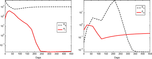
To gain some information on the dynamics of other model states (that is, $H_S$, $H_I$, $E_V$ and $E_K$), we plotted these states versus time in Figure 3, where the results were obtained with parameter values given in Table 4. From this figure, we observe that the number of infected cells (indicated in the left panel) increases at the very beginning and then decreases until it settles down to a small value. This agrees with the viral load data shown in Figure 2 as the only source for production of new virus is from the infected cells. We also observe that the number of BK-specific CD$8+$ T cells $E_V$ (shown in the right panel of Figure 3) increases at the beginning in response to the presence of large amount of free BK virus and then decreases sharply when the viral load decreases to a small level. The trend of increasing-decreasing-increasing of allospecific CD$8+$ T cells $E_K$ (indicated in the right panel of Figure 3) perfectly explains the pattern shown in the serum creatinine data (see the right panel of Figure 2). This is because $E_K$ has a negative effect on the health of the kidney and the damage to the kidney results in increases in the serum creatinine level (as explained in Section 2).

Figure 3. Model solution obtained with parameter values given in Table 4: (left) results for $H_S$ and $H_I$, (right) results for $E_V$ and $E_K$.

4. Concluding remarks and future research effort

Our efforts here to develop a mathematical model with statistically based model validation can be properly viewed as an algorithmic approach to determining the information content in a specific experimental data-set. That is, we illustrate one approach to determining how many and which model parameters can be estimated with confidence from a given data-set. In this context, we have developed a mechanistic mathematical model to describe the immune response to both BKV infection and a donor kidney, and have estimated model parameters and initial conditions using the clinical data. Due to the large number of unknown parameters and limited number of observations, one is unable to reliably estimate all the parameters. To alleviate this difficulty, we employed sensitivity analysis combined with asymptotic theory of estimators to determine the number of parameters that can be reliably estimated. Numerical results show that we were able to reliably estimate five parameters with the given eight viral load data points and sixteen creatinine data points. This clearly demonstrates that one requires more informative longitudinal data, particularly observations on other model variables, in order to fully validate the model. In this context, an immediate future effort would be to use optimal design methods (e.g. [37, 38]) to determine when an experimenter should take measurements and what model variables to measure. The obtained results should then be used to guide the future data collection efforts.

Once we obtain sufficient amount of informative longitudinal data to reliably estimate all the unknown parameters, another immediate future effort is to quantify uncertainties of model response, which is due to uncertainty in parameter estimators. Based on the asymptotic theory, we know that parameter estimators are multivariate normally distributed. Thus, this would involve uncertainty quantification of the system of ordinary differential equations (9(9) $$\begin{array}{cc}\hfill \dot{\mathbf{x}}& =\mathbf{g}(\mathbf{x};\mathbf{p},{\mathbf{x}}_{\mathbf{0}}),\mathbf{x}(\mathbf{0})={\mathbf{x}}_{\mathbf{0}},\hfill \end{array}$$(9) ) driven by a multivariate normally distributed random vector (referred to as a random differential equation). To do this, one could use the fact that the probability density function of solutions to random differential equations is described by the integral of the solution to a hyperbolic partial differential equation with integrator being the cumulative distribution function of a multivariate normally distributed random vector (see [27, Section 7.3.2.2] for details). An alternative approach to do this is to use Monte Carlo methods or other numerical methods such as stochastic Galerkin methods and stochastic collocation methods (e.g. see [27, Section 7.3] and the references therein for details).

Acknowledgements

The authors are grateful to the two anonymous referees for their helpful comments and constructive suggestions which led to an improved version of the paper.

Additional information

Funding

This research was supported in part by [grant number NIAID R01AI071915-10] from the National Institute of Allergy and Infectious Diseases, in part by the Air Force Office of Scientific Research under [grant number AFOSR FA9550-12-1-0188], and in part by the National Science Foundation under Research Training Grant (RTG) [DMS-1246991].

Appendix 1

Results corresponding to the sensitivity analysis conducted during Step 1–Step 4 of the iterative inverse problem algorithm are given in Tables A1–A4.

Table A1. Sensitivity rankings for 29 estimated parameters.

$S_V$	Parameter	$S_C$	Parameter
0	${\mathit{\delta }}_{EK}$	$1.8375\times {10}^{-8}$	${\mathit{\kappa }}_V$
0	${\mathit{\delta }}_{C0}$	$2.5563\times {10}^{-6}$	${\mathit{\lambda }}_{EV}$
0	${\mathit{\lambda }}_{EK}$	$6.1953\times {10}^{-5}$	${\mathit{\kappa }}_{CH}$
0	${\mathit{\lambda }}_C$	$1.4577\times {10}^{-4}$	$E_{V0}$
0	${\mathit{\kappa }}_{EK}$	$1.8694\times {10}^{-4}$	${\mathit{\delta }}_{EH}$
0	${\mathit{\kappa }}_{CH}$	$1.9313\times {10}^{-4}$	${\mathit{\lambda }}_{HS}$
0	${\overline{\mathit{\rho }}}_{EK}$	$5.6584\times {10}^{-4}$	$V_0$
0	${\mathit{\kappa }}_{KH}$	$7.3820\times {10}^{-4}$	$H_{S0}$
0	$E_{K0}$	$1.9130\times {10}^{-3}$	$H_{I0}$
0	$C_0$	$4.1888\times {10}^{-3}$	${\mathit{\delta }}_{EV}$
$4.2652\times {10}^{-3}$	$V_0$	$4.4437\times {10}^{-3}$	${\mathit{\lambda }}_{EK}$
0.016519	$H_{I0}$	0.011330	${\mathit{\delta }}_{HI}$
0.025134	$H_{S0}$	0.019960	${\overline{\mathit{\rho }}}_{EV}$
0.025148	${\mathit{\lambda }}_{EV}$	0.063921	${\mathit{\delta }}_V$
0.087472	${\mathit{\lambda }}_{HS}$	0.071157	${\mathit{\rho }}_V$
1.4476	${\mathit{ϵ}}_4$	0.084435	$\mathit{\beta }$
5.3296	${\mathit{\kappa }}_V$	0.14688	${\mathit{\kappa }}_{HS}$
14.003	$E_{V0}$	0.34333	${\mathit{\kappa }}_{EK}$
15.359	${\mathit{\delta }}_{HI}$	0.42737	$E_{K0}$
18.007	${\mathit{\delta }}_{EH}$	0.51850	${\mathit{\kappa }}_{EK}$
131.04	${\mathit{ϵ}}_1$	0.68038	${\mathit{\delta }}_{C0}$
280.99	${\mathit{\delta }}_V$	1.2403	${\mathit{ϵ}}_4$
282.13	${\mathit{\rho }}_V$	1.3561	${\mathit{ϵ}}_1$
292.00	${\mathit{ϵ}}_3$	3.1602	$C_0$
296.00	${\mathit{\kappa }}_{HS}$	3.5369	${\mathit{ϵ}}_2$
300.73	$\mathit{\beta }$	5.1086	${\mathit{ϵ}}_3$
446.59	${\mathit{ϵ}}_2$	49.962	${\mathit{\lambda }}_C$
1433.4	${\mathit{\delta }}_{EV}$	59.907	${\mathit{\delta }}_{EK}$
4680.9	${\overline{\mathit{\rho }}}_{EV}$	75.318	${\overline{\mathit{\rho }}}_{EK}$

Table A2. Sensitivity rankings for 10 estimated parameters.

$S_V$	Parameter	$S_C$	Parameter
0	${\mathit{\delta }}_{EK}$	0.011400	${\mathit{\delta }}_{EV}$
0	${\overline{\mathit{\rho }}}_{EK}$	0.024951	${\overline{\mathit{\rho }}}_{EV}$
1.0137	${\mathit{\delta }}_V$	0.30254	${\mathit{\delta }}_V$
40.538	${\mathit{ϵ}}_3$	0.34492	${\mathit{\rho }}_V$
171.61	${\mathit{ϵ}}_4$	0.38744	$\mathit{\beta }$
175.47	${\mathit{\kappa }}_{HS}$	0.45276	${\mathit{\kappa }}_{HS}$
205.94	${\mathit{\rho }}_V$	1.8521	${\mathit{ϵ}}_3$
235.60	$\mathit{\beta }$	50.789	${\mathit{ϵ}}_4$
624.14	${\mathit{\delta }}_{EV}$	135.23	${\overline{\mathit{\rho }}}_{EK}$
996.73	${\overline{\mathit{\rho }}}_{EV}$	157.37	${\mathit{\delta }}_{EK}$

Table A3. Sensitivity rankings for 20 estimated parameters.

$S_V$	Parameter	$S_C$	Parameter
0	${\mathit{\delta }}_{EK}$	$1.4997\times {10}^{-7}$	${\mathit{\kappa }}_V$
0	${\mathit{\delta }}_{C0}$	$1.2963\times {10}^{-4}$	$E_{V0}$
0	${\mathit{\lambda }}_C$	$1.9144\times {10}^{-4}$	${\mathit{\delta }}_{EH}$
0	${\overline{\mathit{\rho }}}_{EK}$	0.012164	${\mathit{\delta }}_{EV}$
0	$C_0$	0.026468	${\overline{\mathit{\rho }}}_{EV}$
0.66447	$E_{V0}$	0.029674	${\mathit{\delta }}_{HI}$
1.0155	${\mathit{\delta }}_{EH}$	0.040367	${\mathit{\lambda }}_{HS}$
4.6235	${\mathit{ϵ}}_1$	0.32979	${\mathit{\delta }}_V$
5.7545	${\mathit{\kappa }}_V$	0.37520	${\mathit{\rho }}_V$
12.076	${\mathit{\lambda }}_{HS}$	0.42114	$\mathit{\beta }$
15.216	${\mathit{\delta }}_{HI}$	0.48602	${\mathit{\kappa }}_{HS}$
17.445	${\mathit{ϵ}}_2$	0.64429	${\mathit{ϵ}}_1$
40.518	${\mathit{ϵ}}_3$	1.5687	${\mathit{ϵ}}_2$
173.58	${\mathit{ϵ}}_4$	1.9628	${\mathit{ϵ}}_3$
175.34	${\mathit{\kappa }}_{HS}$	2.2956	$C_0$
183.78	${\mathit{\delta }}_V$	7.8627	${\mathit{\delta }}_{C0}$
205.82	${\mathit{\rho }}_V$	9.0800	${\mathit{\lambda }}_C$
235.35	$\mathit{\beta }$	53.932	${\mathit{ϵ}}_4$
639.54	${\mathit{\delta }}_{EV}$	145.34	${\overline{\mathit{\rho }}}_{EK}$
1022.7	${\overline{\mathit{\rho }}}_{EV}$	168.46	${\mathit{\delta }}_{EK}$

Table A4. Sensitivity rankings for 15 estimated parameters.

$S_V$	Parameter	$S_C$	Parameter
0	${\mathit{\delta }}_{EK}$	0.0097914	${\mathit{\delta }}_{EV}$
0	${\mathit{\delta }}_{C0}$	0.021305	${\overline{\mathit{\rho }}}_{EV}$
0	${\mathit{\lambda }}_C$	0.026802	${\mathit{\delta }}_{HI}$
0	${\overline{\mathit{\rho }}}_{EK}$	0.027472	${\mathit{\lambda }}_{HS}$
10.683	${\mathit{\lambda }}_{HS}$	0.26025	${\mathit{\delta }}_V$
13.489	${\mathit{\delta }}_{HI}$	0.29872	${\mathit{\rho }}_V$
18.399	${\mathit{ϵ}}_2$	0.33683	$\mathit{\beta }$
42.884	${\mathit{ϵ}}_3$	0.37132	${\mathit{\kappa }}_{HS}$
168.53	${\mathit{\kappa }}_{HS}$	1.5572	${\mathit{ϵ}}_2$
174.92	${\mathit{\delta }}_V$	1.7727	${\mathit{ϵ}}_3$
186.84	${\mathit{ϵ}}_4$	7.6471	${\mathit{\delta }}_{C0}$
195.44	${\mathit{\rho }}_V$	8.2445	${\mathit{\lambda }}_C$
223.38	$\mathit{\beta }$	42.258	${\mathit{ϵ}}_4$
688.21	${\mathit{\delta }}_{EV}$	110.23	${\overline{\mathit{\rho }}}_{EK}$
1104.2	${\overline{\mathit{\rho }}}_{EV}$	130.27	${\mathit{\delta }}_{EK}$

Appendix 2

Results corresponding to parameter estimation # 1 associated with estimating 20 parameters are found in Figure B1, Tables B1 and B2. We can see from Figure B1 that the estimate ${\mathit{\theta }}_{\mathrm{opt}}^1$ produced relatively good fits for both the viral and serum creatinine data. However, we observe from Table B2 that the ratio of standard errors to the corresponding estimate, $\mathit{\gamma }$, is huge for all parameters except $C_0$. This means that the estimates for all the parameters except $C_0$ are not reliable. One possible explanation for this result is the size of the condition number of the Fisher information, $\mathit{\chi }{(\widehat{\mathbf{q}})}^T\mathit{\chi }(\widehat{\mathbf{q}})$. In this particular case, it is $2.0604\times {10}^{17}$, obtained using Matlab function cond. This is considerably large and suggests that the matrix is very close to being singular. This presents an issue when calculating the standard errors, since the inverse of the Fisher matrix is required.

Results corresponding to parameter estimation # 2 associated with estimating 15 parameters are found in Figure B2, Tables B1 and B4. Figure B2 also shows relatively good fits for both the viral and serum creatinine data. We observe, however, from Table B4 that $\mathit{\gamma }$ is large for parameters ${\mathit{\lambda }}_{HS},\mathit{\beta },{\overline{\mathit{\rho }}}_{EV},{\mathit{\delta }}_{EV},{\mathit{\delta }}_{EK},{\mathit{\delta }}_{C0},$${\mathit{\kappa }}_{HS},{\mathit{\delta }}_{HI},{\mathit{\rho }}_V,{\overline{\mathit{\rho }}}_{EK},{\mathit{ϵ}}_2,{\mathit{ϵ}}_3,{\mathit{ϵ}}_4$. Yet, $1<\mathit{\gamma }<2$ for ${\mathit{\lambda }}_{HS},{\mathit{\delta }}_{C0}$ and $0.9<\mathit{\gamma }<1$ for ${\mathit{\lambda }}_C$. We note that ${max}_i|{\mathit{\gamma }}_i|=1074.3$, which is much less than that corresponding to parameter estimation # 1. This suggests that there is less uncertainty in the estimates obtained compared to the previous case. It is important to note that the condition number of the Fisher matrix is $1.6620\times {10}^{11}$ and has decreased.

Results corresponding to parameter estimation # 3 associated with estimating 10 parameters are given in Figure B3, Tables B5 and B6. Figure B3 shows relatively good fits for both the viral and serum creatinine data. However, we observe from Table B6 that $\mathit{\gamma }$ is large for parameter ${\mathit{\delta }}_V$, $1<\mathit{\gamma }<4$ for parameters ${\overline{\mathit{\rho }}}_{EV},{\mathit{\delta }}_{EV},{\mathit{\rho }}_V$ and $0.4<\mathit{\gamma }<1$ for parameters $\mathit{\beta },{\mathit{\delta }}_{EK},{\mathit{\kappa }}_{HS},{\overline{\mathit{\rho }}}_{EK},{\mathit{ϵ}}_3,{\mathit{ϵ}}_4$. Note that ${max}_i|{\mathit{\gamma }}_i|=25.924$, which is much less than that corresponding to parameter estimation # 1, 2. This means that we have less uncertainty in parameter estimates compared to that of the other two cases. Similar to the previous two cases, the condition number of the Fisher matrix is $1.9733\times {10}^8$ and has decreased.

Figure B1. Using ${\mathit{\theta }}_{\mathrm{opt}}^1$ in Table B1 for parameter estimation # 1, (Left) Plot of model solution and viral load data on $[0,450]$. (Right) Plot of model solution and serum creatinine data on $[0,450]$.

Table B1. Parameter estimation # 1 results for TOS003 viral load and serum creatinine data on $[0,450]$. Top part (above the horizontal line) of the table gives fixed parameters whereas the bottom part ( below the horizontal line) of the table displays the estimated parameters.

Parameter	${\mathit{\theta }}_{\mathrm{opt}}^1$	Parameter	${\mathit{\theta }}_{\mathrm{opt}}^1$
${log}_{10}{\mathit{\lambda }}_{EV}$	-3.0000	${log}_{10}{\mathit{\lambda }}_{EK}$	-2.6990
${log}_{10}{\mathit{\kappa }}_{EK}$	-0.69897	${log}_{10}{\mathit{\kappa }}_{CH}$	1.0000
${log}_{10}{\mathit{\kappa }}_{KH}$	1.9294	${log}_{10}{H}_{S0}$	3.6990
${log}_{10}{H}_{S0}$	1.7782	${log}_{10}{V}_0$	4.6990
${log}_{10}{E}_{K0}$	-0.39794
${log}_{10}{\mathit{\lambda }}_{HS}$	-1.5291	${log}_{10}\mathit{\beta }$	-7.0633
${log}_{10}{\mathit{\delta }}_{EH}$	-2.7500	${log}_{10}{\mathit{\delta }}_V$	-0.43203
${log}_{10}{\overline{\mathit{\rho }}}_{EV}$	-0.60674	${log}_{10}{\mathit{\delta }}_{EV}$	-0.96806
${log}_{10}{\mathit{\delta }}_{EK}$	-0.99357	${log}_{10}{\mathit{\delta }}_{C0}$	-1.8907
${log}_{10}{\mathit{\kappa }}_{HS}$	3.0032	${log}_{10}{\mathit{\delta }}_{HI}$	-1.0681
${log}_{10}{\mathit{\rho }}_V$	3.6349	${log}_{10}{\mathit{\kappa }}_V$	2.2569
${log}_{10}{\mathit{\lambda }}_C$	-2.1994	${log}_{10}{\overline{\mathit{\rho }}}_{EK}$	-0.78374
${\mathit{ϵ}}_1$	0.10085	${\mathit{ϵ}}_2$	0.36754
${\mathit{ϵ}}_3$	0.60763	${\mathit{ϵ}}_4$	0.35925
${log}_{10}{E}_{V0}$	-1.4234	$C_0$	0.67629

Table B2. Parameter estimates, asymptotic standard errors, confidence intervals and the ratios $\mathit{\gamma }$ of standard error to the corresponding estimate for parameter estimation # 1.

Parameter	Estimate	$SE$	95% CI	$\mathit{\gamma }$
${log}_{10}{\mathit{\lambda }}_{HS}$	-1.5291	321.79	[$-745.52$, 742.46]	210.45
${log}_{10}\mathit{\beta }$	-7.0633	530.68	[$-1.2340\times {10}^3$, $1.2199\times {10}^3$]	75.131
${log}_{10}{\mathit{\delta }}_{EH}$	-2.7500	$7.7607\times {10}^5$	[$-1.7943\times {10}^6$, $1.7943\times {10}^6$]	$2.8221\times {10}^5$
${log}_{10}{\mathit{\delta }}_V$	-0.4320	$6.7490\times {10}^3$	[$-1.5604\times {10}^4$, $1.5603\times {10}^4$]	$1.5622\times {10}^4$
${log}_{10}{\overline{\mathit{\rho }}}_{EV}$	-0.6067	997.13	[$-2.3060\times {10}^3$, $2.3047\times {10}^3$]	$1.6434\times {10}^3$
${log}_{10}{\mathit{\delta }}_{EV}$	-0.9681	$2.0163\times {10}^3$	[$-4.6627\times {10}^3$, $4.6608\times {10}^3$]	$2.0828\times {10}^3$
${log}_{10}{\mathit{\delta }}_{EK}$	-0.9936	$2.5211\times {10}^3$	[$-5.8298\times {10}^3$, $5.8278\times {10}^3$]	$2.5374\times {10}^3$
${log}_{10}{\mathit{\delta }}_{C0}$	-1.8907	254.42	[$-590.10$, 586.32]	134.56
${log}_{10}{\mathit{\kappa }}_{HS}$	3.0032	$1.7893\times {10}^3$	[$-4.1339\times {10}^3$, $4.1399\times {10}^3$]	595.81
${log}_{10}{\mathit{\delta }}_{HI}$	-1.0681	$2.2293\times {10}^3$	[$-5.1553\times {10}^3$, $5.1531\times {10}^3$]	$2.0871\times {10}^3$
${log}_{10}{\mathit{\rho }}_V$	3.6349	$8.7049\times {10}^3$	[$-2.0122\times {10}^4$, $2.0129\times {10}^4$]	$2.3948\times {10}^3$
${log}_{10}{\mathit{\kappa }}_V$	2.2569	$5.6586\times {10}^3$	[$-1.3080\times {10}^4$, $1.3085\times {10}^4$]	$2.5073\times {10}^3$
${log}_{10}{\mathit{\lambda }}_C$	-2.1994	121.88	[$-284.00$, 279.60]	55.416
${log}_{10}{\overline{\mathit{\rho }}}_{EK}$	-0.7837	$2.4214\times {10}^3$	[$-5.5990\times {10}^3$, $5.5974\times {10}^3$]	$3.0895\times {10}^3$
${\mathit{ϵ}}_1$	0.1009	$1.5278\times {10}^3$	[$-3.5321\times {10}^3$, $3.5323\times {10}^3$]	$1.5148\times {10}^4$
${\mathit{ϵ}}_2$	0.3675	128.05	[$-295.69$, 296.43]	348.40
${\mathit{ϵ}}_3$	0.6076	$1.6913\times {10}^3$	[$-3.9097\times {10}^3$, $3.9109\times {10}^3$]	$2.7835\times {10}^3$
${\mathit{ϵ}}_4$	0.3593	142.45	[$-328.99$, 329.71]	396.53
${log}_{10}{E}_{V0}$	-1.4234	$9.3880\times {10}^5$	[$-2.1705\times {10}^6$, $2.1705\times {10}^6$]	$6.5953\times {10}^5$
$C_0$	0.6763	0.16971	[0.28393, 1.0687]	0.25094

Figure B2. Using ${\mathit{\theta }}_{\mathrm{opt}}^2$ in Table B3 for parameter estimation # 2, (Left) Plot of model solution and viral load data on $[0,450]$. (Right) Plot of model solution and serum creatinine data on $[0,450]$.

Table B3. Parameter estimation # 2 results for TOS003 viral load and serum creatinine data on $[0,450]$. Top part (above the horizontal line) of the table gives fixed parameters whereas the bottom part ( below the horizontal line) of the table displays the estimated parameters.

Parameter	${\mathit{\theta }}_{\mathrm{opt}}^2$	Parameter	${\mathit{\theta }}_{\mathrm{opt}}^2$
${log}_{10}{\mathit{\delta }}_{EH}$	-2.7500	${log}_{10}{\mathit{\lambda }}_{EV}$	-3.0000
${log}_{10}{\mathit{\kappa }}_V$	2.2569	${log}_{10}{\mathit{\lambda }}_{EK}$	-2.6990
${log}_{10}{\mathit{\kappa }}_{EK}$	-0.69897	${log}_{10}{\mathit{\kappa }}_{CH}$	1.0000
${log}_{10}{\mathit{\kappa }}_{KH}$	1.9294	${\mathit{ϵ}}_1$	0.10085
${log}_{10}{H}_{S0}$	3.6990	${log}_{10}{H}_{S0}$	1.7782
${log}_{10}{V}_0$	4.6990	${log}_{10}{E}_{V0}$	-1.4234
${log}_{10}{E}_{K0}$	-0.39794	$C_0$	0.67629
${log}_{10}{\mathit{\lambda }}_{HS}$	-1.5205	${log}_{10}\mathit{\beta }$	-7.0671
${log}_{10}{\mathit{\delta }}_V$	-0.43233	${log}_{10}{\overline{\mathit{\rho }}}_{EV}$	-0.60429
${log}_{10}{\mathit{\delta }}_{EV}$	-0.96680	${log}_{10}{\mathit{\delta }}_{EK}$	-0.99302
${log}_{10}{\mathit{\delta }}_{C0}$	-1.8520	${log}_{10}{\mathit{\kappa }}_{HS}$	3.0060
${log}_{10}{\mathit{\delta }}_{HI}$	-1.0704	${log}_{10}{\mathit{\rho }}_V$	3.6344
${log}_{10}{\mathit{\lambda }}_C$	-2.1805	${log}_{10}{\overline{\mathit{\rho }}}_{EK}$	-0.78540
${\mathit{ϵ}}_2$	0.36575	${\mathit{ϵ}}_3$	0.61164
${\mathit{ϵ}}_4$	0.36374

Table B4. Parameter estimates, asymptotic standard errors, confidence intervals and the ratios $\mathit{\gamma }$ of standard error to the corresponding estimate for parameter estimation # 2.

Parameter	Estimate	$SE$	95% CI	$\mathit{\gamma }$
${log}_{10}{\mathit{\lambda }}_{HS}$	-1.5205	2.8635	[-6.7692, 3.7282]	1.8832
${log}_{10}\mathit{\beta }$	-7.0671	64.938	[-126.10, 111.96]	9.1888
${log}_{10}{\mathit{\delta }}_V$	-0.4323	464.46	[-851.79, 850.92]	1074.3
${log}_{10}{\overline{\mathit{\rho }}}_{EV}$	-0.6043	53.623	[-98.895, 97.686]	88.737
${log}_{10}{\mathit{\delta }}_{EV}$	-0.9668	79.892	[-147.41, 145.48]	82.636
${log}_{10}{\mathit{\delta }}_{EK}$	-0.9930	36.222	[-67.388, 65.402]	36.477
${log}_{10}{\mathit{\delta }}_{C0}$	-1.8520	3.7012	[-8.6362, 4.9323]	1.9985
${log}_{10}{\mathit{\kappa }}_{HS}$	3.0060	32.931	[-57.357, 63.369]	10.955
${log}_{10}{\mathit{\delta }}_{HI}$	-1.0704	74.871	[-138.31, 13.617]	69.944
${log}_{10}{\mathit{\rho }}_V$	3.6344	550.96	[-1006.3, 1013.5]	151.60
${log}_{10}{\mathit{\lambda }}_C$	-2.1805	2.0517	[-5.9412, 1.5802]	0.9409
${log}_{10}{\overline{\mathit{\rho }}}_{EK}$	-0.7854	26.666	[-49.664, 48.093]	33.952
${\mathit{ϵ}}_2$	0.3657	10.447	[-18.784, 19.516]	28.564
${\mathit{ϵ}}_3$	0.6116	30.913	[-56.052, 57.275]	50.541
${\mathit{ϵ}}_4$	0.3637	14.389	[-26.011, 26.739]	39.559

Figure B3. Using ${\mathit{\theta }}_{\mathrm{opt}}^3$ in Table B5 for parameter estimation # 3, (Left) Plot of model solution and viral load data on $[0,450]$. (Right) Plot of model solution and serum creatinine data on $[0,450]$.

Table B5. Parameter estimation # 3 results for TOS003 viral load and serum creatinine data on $[0,450]$. Top part (above the horizontal line) of the table gives fixed parameters whereas the bottom part ( below the horizontal line) of the table displays the estimated parameters.

Parameter	${\mathit{\theta }}_{\mathrm{opt}}^3$	Parameter	${\mathit{\theta }}_{\mathrm{opt}}^3$
${log}_{10}{\mathit{\lambda }}_{HS}$	-1.5205	${log}_{10}{\mathit{\delta }}_{EH}$	-2.7500
${log}_{10}{\mathit{\delta }}_{C0}$	-1.8520	${log}_{10}{\mathit{\delta }}_{HI}$	-1.0704
${log}_{10}{\mathit{\lambda }}_{EV}$	-3.0000	${log}_{10}{\mathit{\kappa }}_V$	2.2569
${log}_{10}{\mathit{\lambda }}_{EK}$	-2.6990	${log}_{10}{\mathit{\lambda }}_C$	-2.1805
${log}_{10}{\mathit{\kappa }}_{EK}$	-0.6990	${log}_{10}{\mathit{\kappa }}_{CH}$	1.0000
${log}_{10}{\mathit{\kappa }}_{KH}$	1.9294	${\mathit{ϵ}}_1$	0.1009
${\mathit{ϵ}}_2$	0.3658	${log}_{10}{H}_{S0}$	3.6990
${log}_{10}{H}_{S0}$	1.7782	${log}_{10}{V}_0$	4.6990
${log}_{10}{E}_{V0}$	-1.4234	${log}_{10}{E}_{K0}$	-0.3979
$C_0$	0.6763
${log}_{10}\mathit{\beta }$	-7.0675	${log}_{10}{\mathit{\delta }}_V$	-0.4295
${log}_{10}{\overline{\mathit{\rho }}}_{EV}$	-0.6005	${log}_{10}{\mathit{\delta }}_{EV}$	-0.9635
${log}_{10}{\mathit{\delta }}_{EK}$	-0.9945	${log}_{10}{\mathit{\kappa }}_{HS}$	3.0111
${log}_{10}{\mathit{\rho }}_V$	3.6327	${log}_{10}{\overline{\mathit{\rho }}}_{EK}$	-0.7850
${\mathit{ϵ}}_3$	0.5999	${\mathit{ϵ}}_4$	0.3649

Table B6. Parameter estimates, asymptotic standard errors, confidence intervals and the ratios $\mathit{\gamma }$ of standard error to the corresponding estimate for parameter estimation # 3.

Parameter	Estimate	$SE$	95% CI	$\mathit{\gamma }$
${log}_{10}\mathit{\beta }$	-7.0675	3.1628	[-12.637, -1.4978]	0.44751
${log}_{10}{\mathit{\delta }}_V$	-0.4295	11.135	[-20.038, 19.179]	25.924
${log}_{10}{\overline{\mathit{\rho }}}_{EV}$	-0.6005	1.3981	[-3.0626, 1.8617]	2.3285
${log}_{10}{\mathit{\delta }}_{EV}$	-0.9635	1.9509	[-4.3990, 2.4721]	2.0249
${log}_{10}{\mathit{\delta }}_{EK}$	-0.9945	0.41297	[-1.7218, -0.26729]	0.41524
${log}_{10}{\mathit{\kappa }}_{HS}$	3.0111	1.7573	[-0.083412, 6.1057]	0.58359
${log}_{10}{\mathit{\rho }}_V$	3.6327	12.5245	[-18.423, 25.688]	3.4477
${log}_{10}{\overline{\mathit{\rho }}}_{EK}$	-0.7850	0.40087	[-1.4910, -0.079107]	0.51064
${\mathit{ϵ}}_3$	0.5999	0.59392	[-0.44597, 1.6458]	0.9900
${\mathit{ϵ}}_4$	0.3649	0.22157	[-0.025269, 0.75510]	0.60718

References

- United States department of health and human services, (n.d.). OPTN, SRTR annual report. 2011. p. 8–10. Retrieved May 12, 2014 from the World Wide Web: http://optn.transplant.hrsa.gov.
- Gardner SD, Field AM, Coleman DV, Hulme B. New human papovavirus (B.K.) isolated from urine after renal transplantation. Lancet. 1971;297:1253–1257.
- Heritage J, Chesters PM, McCance DJ. The persistence of papovavirus BK DNA sequences in normal human renal tissue. J. Med. Virol. 1981;8:142–150.
- Hirsch HH. BK virus: opportunity makes a pathogen. Clin. Infect. Dis. 2005;41:354–360.
- Knowles WA, Pipkin P, Andrews N, Vyse A, Minor P, Brown DW, Miller E. Population-based study of antibody to the human polyomaviruses BKV and JCV and the simian polyomavirus SV40. J. Med. Virol. 2003;71:115–123.
- Eash S, Querbes W, Atwood WJ. Infection of vero cells by BK virus is dependent on caveolae. J. Virol. 2004;78:11583–11590.
- Egli A, Binggeli S, Bodaghi S, et al. Cytomegalovirus and polyomavirus BK post-transplant. Nephrol. Dial. Transplant. 2007;22:viii72–viii82.
- Funk GA, Hirsch HH. From plasma BK viral load to allograft damage: rule of thumb for estimating the intrarenal cytopathic wear. Clin. Infect. Dis. 2009;49:989–990.
- Funk GA, Steiger J, Hirsch HH. Rapid dynamics of polyomavirus type BK in renal transplant recipients. J. Infect. Dis. 2006;190:80–87.
- Hammer MH, Brestrich G, Andreee H, et al. HLA type-independent method to monitor polyma BK virus-specific CD4+ and CD8+ T-cell immunity. Am. J. Transplant. 2006;6:625–631.
- Nickeleit V, Hirsch HH, Binet IF, et al. Polyomavirus infection of renal allograft recipients: from latent infection to manifest disease. J. Am. Soc. Nephrol. 1999;10:1080–1089.
- Hirsch HH, Steiger J. Polyomavirus BK. Lancet Infect. Dis. 2003;3:611–623.
- Ramos E, Drachenberg CB, Portocarrero M, et al. BK virus nephrology diagnosis and treatment: experience at the University of Maryland Renal Transplant Program. In: Cecke JM, Terasaki PI, editors. Clinical Transplants. Los Angeles (CA): UCLA Immunogenetics Center; 2002. p. 143–153.
- Banks HT, Tran HT. Mathematical and experimental modeling of physical and biological processes. Boca Raton (FL): Taylor/Francis-Chapman/Hall-CRC Press; 2009.
- Funk GA, Gosert R, Comoli P, Ginevri F, Hirsch HH. Polyomavirus BK replication dynamics in vivo and in silico to predict cytopathology and viral clearance in kidney transplants. Am. J. Transplant. 2008;8:2368–2377.
- Kepler GM, Banks HT, Davidian M, Rosenberg ES. A model for HCMV infection in immunosuppressed patients. Math. Comput. Model. 2005;49:1653–1663.
- Banks HT, Hu S, Jang T, Kwon HD. Modeling and optimal control of immune response of renal transplant recipients. J. Biol. Dyn. 2012;6:539–567.
- Levey AS, Bosch JP, Lewis JB, Greene T, Rogers N, Roth D. A more accurate method to estimate glomerular filtration rate from serum creatinine: a new prediction equation. Ann. Intern. Med. 1999;130:461–470.
- Adams BM, Banks HT, Davidian M, Rosenberg ES. Model fitting and prediction with HIV treatment interruption data. Bull. Math. Biol. 2005;69:563–584.
- Banks HT, Davidian M, Hu S, Kepler GM, Rosenberg ES. Modelling HIV immune response and validation with clinical data. J. Biol. Dyn. 2008;2:357–385.
- Herbeck JT, Mittler JE, Gottlieb GS, Mullins JI. An HIV epidemic model based on viral load dynamics: value in assessing empirical trends in HIV virulence and community viral load. PLOS Comput. Biol. 2014;10:e1003673.
- Herrero-Martinez E, Sabin CA, Evans JG, Griffioen A, Lee CA, Emery VC. The prognostic value of a single hepatitis C virus RNA load measurement taken early after human immunodeficiency virus seroconversion. J. Infect. Dis. 2002;186:470–476.
- Ouma KN, Basavaraju SV, Okonji JA, Williamson J, Thomas TK, Mills LA, Nkengasong JN, Zeh C. Evaluation of quantification of HIV-1 RNA viral load in plasma and dried blood spots by use of the semiautomated cobas amplicor assay and the fully automated cobas Ampliprep/TaqMan assay, version 2.0, in Kisumu, Kenya. J. Clin. Microbiol. 2013;51:1208–1218.
- Carrol RJ, Ruppert D. Transformation and weighting in regression. New York (NY): Chapman & Hall; 1988.
- Davidian M, Giltinan D. Nonlinear models for repeated measurement data. London: Chapman & Hall; 1998.
- Seber GA, Wild CJ. Nonlinear regression. Hoboken (NJ): Wiley; 2003.
- Banks HT, Hu S, Thompson WC. Modeling and inverse problems in the presence of uncertainty. Boca Raton (FL): Taylor/Francis-Chapman/Hall-CRC Press; 2014.
- Randhawa PS, Vats A, Zygmunt D, Swalsky P, Scantlebury V, Shapiro R, Finkelstein S. Quantification of viral DNA in renal allograft tissue from patients with BK virus nephropathy. Transplant. 2002;74:485–488.
- Banks HT, Cintron-Arias A, Kappel F. Parameter selection methods in inverse problem formulation, CRSC Tech. Report CRSC-TR10-03 (2010), NCSU, Raleigh. In: Batzel JJ, Bachar M, Kappel F, editors. Mathematical modeling and Validation in physiology: application to the cardiovascular and respiratory systems. Lecture notes in mathematics. Vol. 2064, Berlin: Springer-Verlag; 2013. p. 43–73.
- Banks HT, Davidian M, Samuels JR Jr, Sutton KL. An inverse problem statistical methodology summary, CRSC Tech. Report CRSC-TR08-01, (2008), NCSU, Raleigh. In: Chowell G, Hyman M, Hengartner N, Bettencourt LMA, Castillo-Chavez C, editors. Statistical Estimation Approaches in Epidemiology. Berlin, Heidelberg, New York: Springer; 2009. p. 249–302.
- Banks HT, Dediu S, Ernstberger SL, Kappel F. Generalized sensitivities and optimal experimental design, center for research in scientific computation report, CRSC-TR08-12 (revised) (2008), NCSU, Raleigh. J. Inverse Ill-Posed Prob. 2010;8:25–83.
- Banks HT, Holm KJ, Kappel F. Comparison of optimal design methods in inverse problems technical report CRSC-TR10-11 (2010), NCSU, Raleigh. Inverse Prob. 2011;27:075002.
- Özisik MN, Orlande HRB. Inverse heat transfer: fundamentals and applications. New York (NY): Taylor & Francis; 2000.
- Banks HT, Holm K, Robbins D. Standard error computations for uncertainty quantification in inverse problems: asymptotic theory vs. bootstrapping, CRSC technical report CRSC-TR09-13, NCSU, May 2010, Math. Comput. Model. 2010;52:1610–1625.
- Efron B, Tibshirani RJ. An introduction to the bootstrap. Boca Raton (FL): Chapman & Hall/CRC Press; 1998.
- Steyerberg EW, Harrell FE Jr, Borsboom GJJM, Eijkemans MJC, Vergouwe Y, Habbema JF. Internal validation of predictive models: efficiency of some procedures for logistic regression analysis. J. Clin. Epidemiol. 2001;54:774–781.
- Banks HT, Rehm KL. Experimental design for vector output systems, CRSC technical report CRSC-TR12-11, April 2012. Inverse Prob. Sci. Eng. 2013;22:1–34. doi:10.1080/17415977.2013.797973
- Banks HT, Rehm KL. Experimental design for distributed parameter vector systems, CRSC technical report CRSC-TR12-17, August 2012. Appl. Math. Lett. 2013;26:10–14. http://dx.doi.org/10.1016/j.aml.2012.08.003.