Migration NSGA: method to improve a non-elitist searching of Pareto front, with application in magnetics

Abstract

The paper describes a migration strategy to improve classical non-dominated sorting genetic algorithm (NSGA) to find optimal solution of a multi-objective problem. Migration NSGA has been tested to assess its performance using analytical functions for which the Pareto front is known in analytical form, as well as two case studies in electromagnetics, for which the Pareto front is not known a priori. This strategy improves the approximation of the Pareto-optimal solutions of a multi-objective problem by introducing new individuals in the population miming the effect of migrations.

Keywords:

• non-dominated sorted algorithm
• multi-objective optimization
• Pareto front
• analytical problem
• magnetic case study

Introduction

Over the past two decades, evolutionary algorithms have proven good performance when solving optimization problems in the area of computational electromagnetics, like problems of optimal shape design or material property identification.[1–10] Biogeography is the study of the geographic distribution of biological organisms which is observed in nature. Mathematical models of biogeography inspired a class of derivative-free optimization algorithms aiming to find an optimum balance between immigrating and emigrating populations in an island.[4,11–15]

NSGA is an algorithm that mimics the evolution of a population with internal selection of better individuals.[1,6,16–21] NSGA has proven to be effective with high number of individuals and generations. In fact, it works well if the evaluation of objective functions is less time-consuming, allowing the management of a large number of individuals. This characteristic makes NSGA a popular optimization algorithm to find Pareto front of problems that foresee low computational costs to evaluate the objective functions, for instance, when the objective functions are described by simple analytical models. Nevertheless, NSGA suffers of some drawbacks when the population and number of iteration must be limited to reduce the time computation: it can occur, e.g. when the objective functions are evaluated using a numerical method like finite element. Moreover, when the number of individuals in the initial population is limited, the solution is sometimes affected by the choice of the initial population. This phenomenon is described in the next section with an example.

Some authors have proposed modifications of NSGA algorithm to improve convergence or quality of solutions, mostly avoiding elitist searching paths that can occur when only the best fitted individuals are selected by the algorithm.[22,23] In this paper, a straightforward correction to a standard NSGA-II [5,6,17,24,25] in terms of a migrating population is proposed.

The concept of migration has been already implemented in other similar optimization algorithms, mostly applied to strategies that make use of parallel computing. In this algorithm, migration concept is referred to exchange of individuals that evolve autonomously in independent islands.[26–29] In turn, ‘island’ paradigms mimic the behaviour of separate populations (or demes) that evolve without exchanges with neighbours. This might occur within oceanic islands where distances strongly limit the movements of populations. Although each island evolves under seclusion conditions for most of the run, individuals occasionally migrate between islands on the basis of some selection or fitness criteria. This concept of migration allows relatively strong gene mixing within each deme, but it restricts gene flow between different demes or islands. At the end of the optimization run, each ‘island’ selects a subset of population that can contribute to a part of the Pareto front of the problem.[26] Other strategies that include a migration concept can be found in the class of self-organizing migrating algorithms.[30,31] In this case, it is the population that ‘migrates’ and there is not any inclusion of new individuals in the current population. Furthermore, among multi-objective algorithms, particle swarm optimization is a class of algorithms that simulate the movement of swarms of birds or bees [15,32,33] in searching for food. Like in NSGA-II, also this algorithm presents some drawbacks and some modifications have been recently proposed [14] in order to upgrade diversity, e.g. a scout element performs a random search of food exploring different regions, and to improve algorithm performances.[34]

In this paper, it is assumed that migration of a new population occurs systematically during the run of optimization process. When the immigration of a new population occurs, the algorithm imposed a subsequent emigration to keep the number of individuals almost constant. Immigration of new individuals can happen in two different steps of NSGA algorithm, leading to two different approaches of MNSGA. In the first approach, new individuals arrive after the implemented genetic algorithm (GA) has already created a new population of parents and offspring. In the second approach, immigrated individuals are mixed to the parents and actively contribute in defining the new generation of parents and offspring.

These two variants of NSGA have been tested on four problems in order to assess the performances of the proposed algorithm, mostly in terms of Pareto front estimation, with respect to the performance of non-modified NSGA II. The first and second test case makes use of an analytical problem with two objective functions for which the equation of the Pareto front is known. The third test case is an identification problem in magnetics, where experimental data are fitted using a parametric mathematical model. In this case, the Pareto front is not known a priori and the results are compared to the once obtained using classical NSGA-II optimization algorithm starting from the same initial set of individuals. Finally, a case study dealing with the design optimization of a power inductor for magneto fluid heating is developed.

The new algorithms were able to improve the estimation of Pareto front in problems for which the computational cost of the objective functions is substantially high, so that only a relatively small number of individuals are adopted for each generation.

Typical drawback of classical NSGA-II

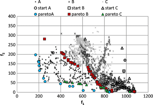
In recent years, NSGA-II algorithm has been coupled to finite element analysis (FEA) where objective functions are obtained from numerical solutions of field equations. For the sake of an example, let the optimal design of an induction-heating device be considered. The optimization objectives are the magnetic field in-homogeneity in a control region and the sensitivity of solutions. This case is presented because NSGA has shown several limitations in finding the Pareto front. In fact, Figure 1 shows three optimization results of the same electromagnetic FEA problem [35,36] obtained using NSGA-II algorithm and starting from three different initial sets of individuals (number of generations 50, number of individuals in the initial set 20). Symbols of squares, circle and triangle represent the three different Pareto fronts obtained. It can be seen that the obtained fronts are different and they do not represent the real Pareto front of the problem.

Figure 1. Three different Pareto fronts and relevant starting individual sets for the same optimization problem. f₁ is the magnetic field uniformity and f₂ is the solution sensitivity. Both quantities are dimensionless.

Migration NSGA

Migration NSGA (MNSGA) mimics the event of a suddenly increased population because of the arrival of a group of individuals that may have different characteristics with respect to originating population. The new individuals, generated through a random process like the one applied to create the initial population, may carry different genes that can be integrated within the original population. In this way, the genetic heritage of the population can mutate.

MNSGA can operate with two different strategies sketched in Figures 2 and 3. The first approach, MNSGA-1, is presented in Figure 2. The immigrated population is added after the main genetic operator (i.e. cross-over + mutation) and before the selection operator. In this way, the immigrants are added to the existing population of parents and offspring and selection operates in such a way that, among the new individuals, only the ones with better characteristics are inserted in the population resulting after selection.

Figure 2. The flow chart of the first variant of migration NSGA algorithm: MNSGA-1; the migration occurs after the genetic operator.

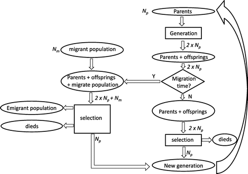
Figure 3. The flow chart of the second variant of migration NSGA algorithm: M-NSGA-2; the migration occurs before the genetic operator.

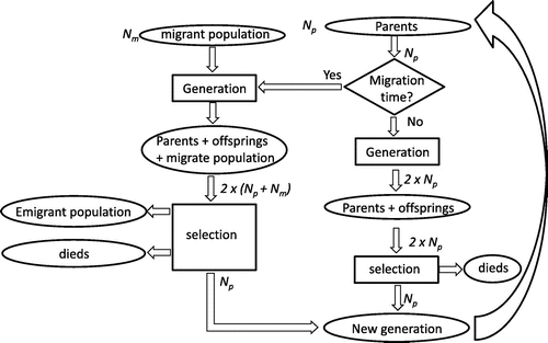
The concept of the second approach for MNSGA-2 is presented in Figure 3. The immigrated population is added to the parents selected in the previous run before the main genetic operator. In this way, the new individuals are mixed with the existing parents to create a new larger population to whom the genetic operator is applied. Genetic characteristics of immigrated population are immediately mixed with the ones of the original population.

The migration of a population is ruled by two parameters:

T_m = the period of migration with respect to the number of iteration (e.g. T_m = 1 is equivalent to introduce a migration at every iteration).

N_m = the number of individuals in the migrated population.

The number of individuals after selection is maintained constant by applying selection and emigration events. The emigration step is managed in the selection algorithm, intended as the step that reduces the population dimensionality. In fact, among the eliminated individuals, a subgroup of individuals dies and a subgroup emigrates. In both cases, some individuals drop out from the current population during the selection step of the NSGA algorithm.

Rationale of migration strategy

Like it occurs in natural populations, where groups of external individuals can immigrate in an existing population in an island, also emigration of groups of individuals from the island should take place to reach a sustainable balance. In fact, computational biogeography models the process of natural immigration and emigration of species between islands in the search for more friendly habitats, which is observed in nature. In computational electromagnetics, applications of biogeography-based optimization (BBO) [4] are an emerging new field of research; accordingly, various problems of optimal design have been successfully solved.[37–39] Although BBO is a population-based algorithm, it does not involve the generation of offspring from given parents like it happens in GAs. Our proposal of MNSGA does not change the evolutionary behaviour of the basic optimization algorithm: we simply suggest a possible interpretation of the migration event in terms of biogeographical concepts. In particular, in both implementations of MNSGA discussed in the previous sections, the emigration is interpretable as a special selection operator to maintain a number of individuals constant in the population.[2,4,40]

Numerical tests

In this section, the two problems used to test the performance of the two MNSGA strategies are described.

Problem #1a: analytical problem

The test problem named problem #1a comprises two design variables, (x₁, x₂), and two objective functions (f₁, f₂) to be minimized. The domain of the design variable varies in a prescribed range, x₁ = [0, 2]; x₂ = [0, 2]. The objective functions are:

(1) $$f_1=x_1^2+x_2^2$$(1)

(2) $$f_2={\left(x_1-1\right)}^2+{\left(x_2-1\right)}^2$$(2)

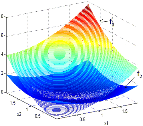
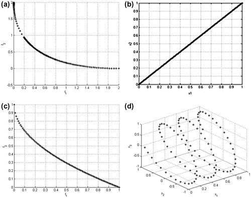
Figure 4 shows the shape of f₁ and f₂ functions in the domain, that is interval [0, 2], whereas Figure 5(a) reports the Pareto front obtained searching for a minimum of the pair (f₁, f₂). Figure 5(b) presents the inverse image of the front. The analytical solution of the front is:

Figure 4. Test problem #1a: shape of the f₁ and f₂ functions in the domain.

Figure 5. Test problem #1: (a) and (c) analytical Pareto front and (b) and (d) analytical inverse image of Pareto front for problem #1a and #1b, respectively.

(3) $$f_2-f_1+2\sqrt{2}\sqrt{f_1}-2=0$$(3)

whereas the one of the inverse image is simply:

(4) $$x_1-x_2=0.$$(4)

Problem #1b: analytical problem

The second analytical problem considers three design variables, (x₁, x₂, x₃), and two objective functions (f₁, f₂) to be minimized. The domain of the design variable vary in a prescribed range, x₁ = [0, 1] and x₂ = x₃ = [−1, 1]. The objective functions are [41]:

(5) $$f_1=x_1+\frac{2}{3}{\left[x_3-sin(6\mathit{\pi }{x}_1+\mathit{\pi })\right]}^2$$(5)

(6) $$f_2=1-\sqrt{x_1}+{\left[x_2-sin\left(6\mathit{\pi }{x}_1+\frac{2}{3}\mathit{\pi }\right)\right]}^2$$(6)

The analytical expressions of the Pareto front and inverse image are, respectively:

(7) $$f_2-1+\sqrt{f_1}=0$$(7)

(8) $$\left\{\begin{array}{c}{x}_2-sin\left(6\mathit{\pi }{x}_1{x}_2+\frac{2}{3}\mathit{\pi }\right)=0\hfill \\ x_3-sin\left(6\mathit{\pi }{x}_1{x}_2+\frac{2}{3}\mathit{\pi }\right)=0\hfill \end{array}\right.$$(8)

Problem #2.1: identification of magnetic material property – direct problem

The second test represents an electromagnetic case study that makes use of analytical equations for the solution of the electromagnetic problem to evaluate objective functions. The optimization problem concerns the numerical identification of the B–H curve of a magnetic material.[42–44] The following model of the B–H curve is assumed:

(8) $$B(H)={\mathit{\mu }}_{0}H+B_S\frac{H_a+1-\sqrt{{\left(H_a+1\right)}^2-4H_a\left(1-a\right)}}{2\left(1-a\right)}$$(8)

with

(9) $$H_a=\frac{{\mathit{\mu }}_0\left({\mathit{\mu }}_r-1\right)H}{B_s}$$(9)

where μ₀ is the magnetic permeability of vacuum, μ_r is the initial relative magnetic permeability (varying between 1 and 5 × 10³), H is the magnetic field, B is the magnetic flux density, B_s is the magnetic flux density at saturation (varying between 0.5 and 2 T) and a is the parameter (a value between 0 and 0.5) that modifies the shape of knee of the B–H curve. This problem has not any analytical solution for the Pareto front and its inverse image.

Problem #2.2: identification of magnetic material property – inverse problem

Given the analytical description of the B–H curve in (8(8) $$B(H)={\mathit{\mu }}_{0}H+B_S\frac{H_a+1-\sqrt{{\left(H_a+1\right)}^2-4H_a\left(1-a\right)}}{2\left(1-a\right)}$$(8) ), the vector x of design variables describes the three parameters that define the model (magnetic flux density at saturation, B_s, initial relative magnetic permeability, μ_r, and knee parameter, a, x = (B_s, μ_r, a)). When a set of values, measured or calculated, of magnetic field and corresponding magnetic flux density is known, the first objective function is defined as the discrepancy between measurements and model estimation:

(10) $$f_1(\mathit{x})\equiv {∥B-\tilde{B}∥}_{\infty }=\underset{H}{sup}\left|B(H,\mathit{x})-\tilde{B}\left(H\right)\right|$$(10)

In this example, we consider known values as not affected by uncertainty. The second objective is the sensitivity with respect to design variables, computed by differentiating the (8(8) $$B(H)={\mathit{\mu }}_{0}H+B_S\frac{H_a+1-\sqrt{{\left(H_a+1\right)}^2-4H_a\left(1-a\right)}}{2\left(1-a\right)}$$(8) ) with respect to each design variable and computing the root mean square of the three partial derivatives:

(11) $$f_2(x)=\sqrt{\sum _{i=1}^3{\left(\frac{\mathit{\partial }B(H)}{\mathit{\partial }{x}_i}\right)}^2}$$(11)

Both the objective functions (10(10) $$f_1(\mathit{x})\equiv {∥B-\tilde{B}∥}_{\infty }=\underset{H}{sup}\left|B(H,\mathit{x})-\tilde{B}\left(H\right)\right|$$(10) )–(11(11) $$f_2(x)=\sqrt{\sum _{i=1}^3{\left(\frac{\mathit{\partial }B(H)}{\mathit{\partial }{x}_i}\right)}^2}$$(11) ) have to be minimized.

Problem #3.1: finite element-based case study – direct problem

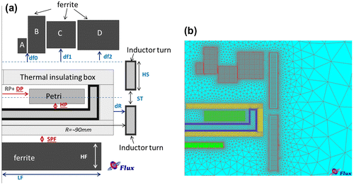
The 2D axisymmetric geometry sketched in Figure 6 shows a device to generate a uniform magnetic field in the bottom of a Petri dish placed in a thermally insulated box. The magnetic field source is an inductor with two turns and five ferrite blocks in order to concentrate the magnetic flux lines in the Petri dish bottom and placed as in Figure 6. The magnetic field problem is solved in time-harmonic conditions by means of a finite element code (e.g. FLUX2D manufactured by Cedrat [45]). The direct problem is solved in terms of the phasor of magnetic vector potential, A, coupled with the electric scalar potential, V. When the Coulomb gauge is applied on the magnetic vector potential, i.e. $\mathrm{\nabla }·\dot{\mathit{A}}=0$, the following coupled equations are solved [18,20,21,36,46,47]:(12) $$\mathrm{\nabla }\times {\mathit{\mu }}^{-1}\mathrm{\nabla }\times \dot{\mathit{A}}+j\mathit{\omega }\mathit{\mu }{\mathit{\rho }}^{-1}\dot{\mathit{A}}=-{\mathit{\rho }}^{-1}\mathrm{\nabla }\dot{V}$$(12) (13) $$\mathrm{\nabla }·{\mathit{\rho }}^{-1}(j\mathit{\omega }\mathit{\mu }\dot{\mathit{A}}+\mathrm{\nabla }\dot{V})=0$$(13)

Figure 6. (a) Geometry of the device with eight design variables and three uncertain parameters (parameters underlined). (b) Mesh detail.

with ρ and μ are the resistivity and permeability, respectively, of the copper and ω field pulsation. The inductor has been supplied imposing a voltage of 600 V_rms at 350 kHz. The mesh has 23,000 nodes and 13,000 elements (Figure 6(b)).

Problem #3.2: finite element-based case study – inverse problem

The bi-objective inverse problem has eight design variables (‘dR’ is the coil distance from the insulated box; ‘HS’ is the vertical size of the inductor turns; ‘ST’ is the turn gap; ‘hf₀’, ‘hf₁’ and ‘hf₂’ are the vertical distances of the four ferrite blocks from the insulated box; ‘HF’ and ‘LF’ are the sizes of ferrite block under the Petri) shown in Figure 6 and aims at minimizing [36]:

I.	(f1): the inhomogeneity of the magnetic field, H, on the bottom of the Petri dish (f1), evaluated as in [20,21,24,36] with a tolerance interval of ±10 A/m;
II.	(f2): the sensitivity of f1 with respect to a set of three uncertain parameters [20,36] (‘DP’ is the Petri dish radial position, ‘SPF’ is the vertical distance of insulated box from lower ferrite and ‘HP’ is the vertical position of the Petri dish from the insulated box bottom).

A detailed description of the used objective functions is in [20,36]. The inverse problem has been solved using both the MNSGA-1 algorithm and a classical NSGA-II non-dominated sorting GA including design of experiment strategy for the evaluation of the solution sensitivity.[20]

Evaluation of algorithm performances in problem #1

Given the problem #1, the performances of MNSGA algorithm are compared to the ones of the classical NSGA-II algorithm. The performance test has been performed varying both migration parameters, N_m and T_m (the number of individuals migrated and the period of migration), and varying also the main parameters of GA as the number of individuals in the initial generation, N_p, (e.g. 20 or 50) and the number of generations, N_g, (e.g. 20 or 50). The tests have been performed starting from some different initial sets of individuals, and of course, these initial sets have been used in all the optimization processes for the comparison.

To evaluate the computational cost of the different algorithms, the maximum number of individuals evaluated for selection has been computed:

(14) $$N_{\text{NSGA}}=N_p+N_g\times N_p$$(14)

Equation (14(14) $$N_{\text{NSGA}}=N_p+N_g\times N_p$$(14) ) represents an estimation of the maximum number of individuals created using NSGA-II algorithm. Considering the event of immigration, the number of individuals increases as in (15(15) $$N_{\text{MNSGA}}=N_p+N_g\times N_p+\frac{N_g}{T_m}\times N_m$$(15) ) where a third term is added to include N_m more individuals. The ratio N_g/T_m represents the number of migratory event. Then, the third term represents the number of individuals generated at each time that one of the N_g/T_m migration event occurs:

(15) $$N_{\text{MNSGA}}=N_p+N_g\times N_p+\frac{N_g}{T_m}\times N_m$$(15)

Non-modified NSGA-II algorithm requires the selection among $N{}_p^{\prime }$ individuals per generation, while in the migration algorithm, N_p individuals per generation must be evaluated for selection, fixing N_g, N_m, and T_m and equalling the total number of individuals created using NSGA-II algorithm (Equation (14(14) $$N_{\text{NSGA}}=N_p+N_g\times N_p$$(14) )) and migration strategy (Equation (15(15) $$N_{\text{MNSGA}}=N_p+N_g\times N_p+\frac{N_g}{T_m}\times N_m$$(15) )) it turns out to be:

(16) $$N_p<N_p^{\prime }-\left(\frac{N_g}{T_m}\times N_m\right)\times \frac{1}{1+N_g}$$(16)

Consequently, the proposed migration strategies require fewer individuals per generation with respect to the NSGA-II algorithm because some individuals are added during the process.

Some metrics are introduced in the literature in order to quantify the performance of the proposed algorithms and compare them with the results obtained with other algorithms.[48–50] In particular, in this paper, metrics that quantify the error between the approximated and exact front, composed of N_k individuals and correspondent inverse image have chosen. Considering the design variable space and the N_k elements of the approximated and exact inverse image of the lower rank final front, the geometric distance of each k-th point (x₁,_k, … , x_V,k) is

(17) $$d_{x,k}=\sqrt{\sum _{i=2}^V{(x_{i,k}-ı{\mathit{f}}_i^{-1}(x_{1,k},\dots ,x_{V,k}))}^2}$$(17)

where $\mathit{f}{}_i^{-1}$ is the i-th component of the inverse image of the Pareto front.

Whereas considering the N_k elements in objective space, the error d_f,k is evaluated computing f₂ given the value of f₁ using (3(3) $$f_2-f_1+2\sqrt{2}\sqrt{f_1}-2=0$$(3) ) or (7(7) $$f_2-1+\sqrt{f_1}=0$$(7) ) [1]:

(18) $$d_{f,k}=\left|f_{2,k}-f_{2,k}(f_{1,k})\right|$$(18)

As far as error metrics is concerned, for each individual of the final front formed by N_k elements, the (17(17) $$d_{x,k}=\sqrt{\sum _{i=2}^V{(x_{i,k}-ı{\mathit{f}}_i^{-1}(x_{1,k},\dots ,x_{V,k}))}^2}$$(17) ) and (18(18) $$d_{f,k}=\left|f_{2,k}-f_{2,k}(f_{1,k})\right|$$(18) ) have been evaluated and a two sets of ‘error vectors’ have been generated. Both the maximum and the rms value of each ‘error vector’ are searched for:(19) $$er{r}_{\text{max}}\left(a\right)=\text{max}(d_{a,k})a=x\text{or}f$$(19) (20) $$er{r}_{\text{rms}}\left(a\right)=\sqrt{\frac{1}{N_k}\sum _{k=1}^{N_k}{d}_{a,k}^2}a=x\text{or}f$$(20)

The crowding distance, i.e. the number of individuals close to the individual k-th of the front, has been also evaluated for both the objective and design variable spaces. The average distances σ_x and σ_f correspond to the design variables and objective spaces and have been computed as:

(21) $${\mathit{\sigma }}_a=\frac{1}{N_k-1}\sqrt{\sum _{i=1}^{N_a}{(max\left(a_i\right)-\text{min}(a_i))}^2}$$(21)

With a = x or f and N_a = length (a). Given the individual k-th of the front, its distance from other individuals of the front is computed as:(22) $$d_a(k,j)=\sqrt{\sum _{q=1}^{N_a}{\left[\frac{a_{k,q}-a_{j,q}}{max\left(a_q\right)-\text{min}(a_q)}\right]}^2}j\ne k,j=1,\dots N_k$$(22)

With N_a the number of design variables (N_x = 2 if V = 2 or N_x = 3 if V = 3) or objective functions (N_f = 2).

The crowding of the front in terms of design variables or objective spaces, cw_a (k) with a = x or f, is the number of individuals, j-th, close to the individual k-th given the distance (22(22) $$d_a(k,j)=\sqrt{\sum _{q=1}^{N_a}{\left[\frac{a_{k,q}-a_{j,q}}{max\left(a_q\right)-\text{min}(a_q)}\right]}^2}j\ne k,j=1,\dots N_k$$(22) ), d_a (k, j), and the threshold (21(21) $${\mathit{\sigma }}_a=\frac{1}{N_k-1}\sqrt{\sum _{i=1}^{N_a}{(max\left(a_i\right)-\text{min}(a_i))}^2}$$(21) ), σ_a:

(23) $$c{w}_a\left(k\right)=\sum _{j=1}^{N_k}{U}_{k,j}\text{with}U(k,j)=\left\{\begin{array}{c}1\text{if}{d}_a(k,j)<{\mathit{\sigma }}_a\\ 0\text{if}{d}_a(k,j)\ge {\mathit{\sigma }}_a\end{array}\right.$$(23)

Results for problem #1a and #1b

Figure 7 shows the optimization results of problem #1a obtained by means of the classical NSGA-II algorithm searching for the pairs (x₁, x₂) that give the best approximation of the Pareto front (3).

Figure 7. (a) Pareto front and (b) design variable space representation obtained using NSGA-II algorithm considering a population of N_p = 20 individuals, N_g = 20 generations and three different initial sets of design variables. (c) Pareto front and (d) design variable space representation obtained using NSGA-II algorithm considering N_p = 50 individuals, N_g = 20 generations and three different initial sets of design variables.

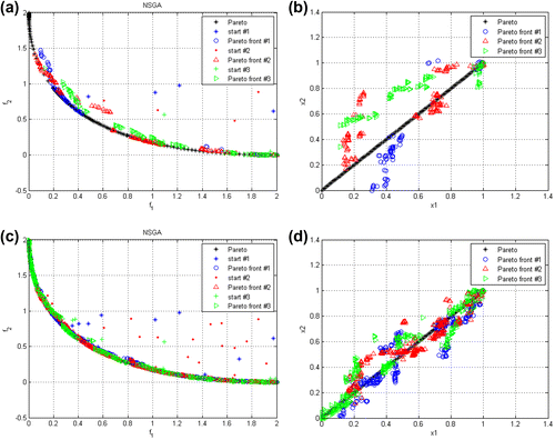
Figure 7(a) and (c) represents the estimated Pareto fronts using classical NSGA-II algorithm. For these cases, 20 generations (N_g = 20) have been considered starting from three different sets of initial individuals and varying the number of individuals in the initial set (N_p = 20 (Figure 7(a)) or N_p = 50 (Figure 7(b))). Figure 7(b) and (d) represents the solutions on Pareto front as a function of design variables. It can be observed that for larger N_p, the estimated Pareto front can be a good approximation of the real one. Approximated Pareto fronts calculated with a lower number of individuals N_p exhibit a worst approximation of the real one.

Figures 8 and 9 report the Pareto front calculated with the classical NSGA approach and the new migration approach for the case of 20 generations (N_g = 20) starting from two different initial sets of 20 individuals (N_p = 20) in terms of objective and design variable spaces. The migration period is 5 (T_m = 5) in Figure 8 and 2 (T_m = 2) in Figure 9. The number of migrated individuals is 10 (N_m = 10). In this case, the maximum number of individuals evaluated using the different optimization algorithms are, respectively, N_NSGA = 420, N_M-NSGA-1 = 500 and N_M-NSGA-2 = 500.

Figure 8. Comparison of (a) the Pareto front obtained using classical NSGA-II, MNSGA-1 and MNSGA-2 algorithm considering N_g = 20, N_p = 20, N_m = 10, and T_m = 5. (b) Comparison of the design variable space obtained using classical NSGA-II, MNSGA-1 and MNSGA-2 algorithms. Crowding distance on (c) objective space and (d) on design variable space.

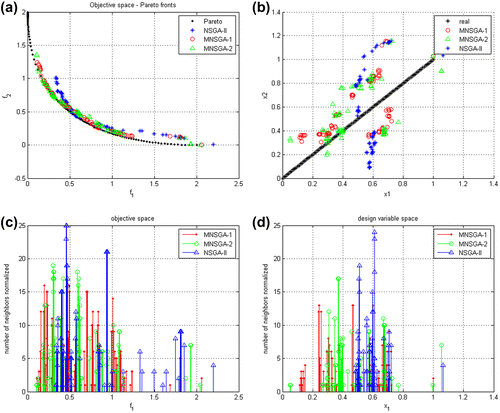
Figure 9. Comparison of (a) the Pareto front obtained using classical NSGA-II, MNSGA-1 and MNSGA-2 algorithm considering N_g = 20, N_p = 20, N_m = 20, and T_m = 5. (b) Comparison of the design variable space obtained using classical NSGA-II, MNSGA-1 and MNSGA-2 algorithms. Crowding distance on (c) objective space and (d) on design variable space.

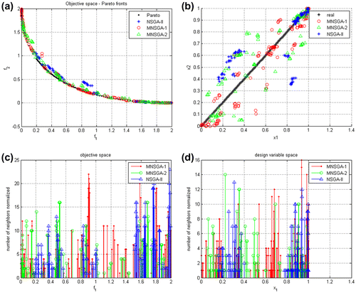
Panel (b) of Figures 8 and 9 compares the inverse images of solutions on the Pareto front using the algorithms NSGA-II, MNSGA-1 and MNSGA-2 with real inverse image. Finally, panels (c) and (d) of Figures 8 and 9 show the crowding distance evaluated using (23(23) $$c{w}_a\left(k\right)=\sum _{j=1}^{N_k}{U}_{k,j}\text{with}U(k,j)=\left\{\begin{array}{c}1\text{if}{d}_a(k,j)<{\mathit{\sigma }}_a\\ 0\text{if}{d}_a(k,j)\ge {\mathit{\sigma }}_a\end{array}\right.$$(23) ) considering the objective space and the design variable space, respectively.

Figure 10 reports the comparison between the classical NSGA approach and the new migration approach for the case N_g = 50 starting from an initial sets of 20 individuals (N_p = 20) in terms of objective and design variable spaces. The migration period is 2 (T_m = 2) and the number of migrated individuals, N_m, is 10. In this case, the maximum number of individuals evaluated using the different optimization algorithms is for the case with N_m = 10 are N_NSGA = 1020, N_MNSGA-1 and N_MNSGA-2 = 1220, respectively. It can be noted that the 1020 individuals evaluated using the classical NSGA-II algorithm are not sufficient to identify the entire Pareto front. A better estimation is obtained computing 1120 or 1220 by means of MNSGA algorithms.

Figure 10. Comparison of (a) the Pareto front obtained using classical NSGA-II, MNSGA-1 and MNSGA-2 algorithm considering N_g = 50, N_p = 20, N_m = 10, and T_m = 2. (b) Comparison of the design variable space obtained using classical NSGA-II, MNSGA-1 and MNSGA-2 algorithms. Crowding distance on (c) objective space and (d) on design variable space.

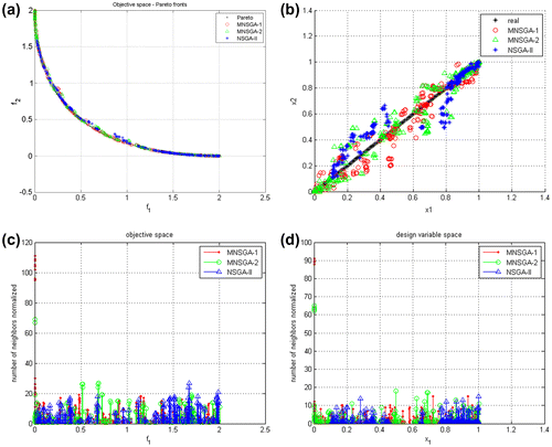
Panel (b) of Figure 10 compares the inverse images of solutions on the Pareto front using the algorithms NSGA-II, MNSGA-1 and MNSGA-2 with real inverse image. Finally, panels (c) and (d) of Figure 10 show the crowding distance evaluated using (23(23) $$c{w}_a\left(k\right)=\sum _{j=1}^{N_k}{U}_{k,j}\text{with}U(k,j)=\left\{\begin{array}{c}1\text{if}{d}_a(k,j)<{\mathit{\sigma }}_a\\ 0\text{if}{d}_a(k,j)\ge {\mathit{\sigma }}_a\end{array}\right.$$(23) ) considering the objective space and the design variable space, respectively.

Figure 11 reports the results obtained using the pairs of objective functions of the problem #1b.

Figure 11. Comparison of the Pareto front and the design variable space obtained using classical NSGA-II, MNSGA-1 and MNSGA-2 algorithm considering N_g = 20, N_p = 20, N_m = 10 (a) and (e) T_m = 2 and (b) and (f) T_m = 5. Crowding distance on (c) and (g) objective space and (d) and (h) on design variable space for T_m = 2 and 5, respectively.

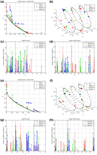
As far as the crowding distance is concerned, both the proposed variations of the NSGA algorithm give a better distribution of solutions along the front and, consequently, a lower crowding distance. This demonstrates that migration strategy improves a non-elitist search of the Pareto front.

Table 1 reports the results of the tests performed on the analytical case. For each test, the number of generations, N_g, of the individuals in the population, N_p, and in the migrated population, N_m, as well as the migration period, T_m, is indicated. Tests are the run starting from 30 different initial populations. For each optimization algorithm, the average rms error of the points belongs to the Pareto front and corresponding inverse image, evaluated using (19(19) $$er{r}_{\text{max}}\left(a\right)=\text{max}(d_{a,k})a=x\text{or}f$$(19) ) and (20(20) $$er{r}_{\text{rms}}\left(a\right)=\sqrt{\frac{1}{N_k}\sum _{k=1}^{N_k}{d}_{a,k}^2}a=x\text{or}f$$(20) ), respectively, has been reported. It appears that the average rms error found applying NSGA-II algorithm is greater than the one found applying the both the MNSGA algorithm. Moreover, increasing the number of generations reduces the rms error. The rms error found in problem #1a is lower than the one in problem #1b.

Table 1. Results of the tests performed: average of the rms error evaluated on inverse image using (19) and objective space using (20) of 30 optimization runs.

	f_objective		Np	Ng	Pm	Tm	errrms(x)	errrms(f)
Case #1	(1) and (2)	NSGA	20	20	–	–	0.21	0.08
		MNSGA_1	20	20	10	5	0.17	0.05
		MNSGA_2	20	20	10	5	0.15	0.04
Case #2	(1) and (2)	NSGA	20	20	–	–	0.34	0.14
		MNSGA_1	20	20	10	2	0.41	0.20
		MNSGA_2	20	20	10	2	0.33	0.14
Case #3	(1) and (2)	NSGA	20	50	–	–	0.12	0.04
		MNSGA_1	20	50	10	5	0.08	0.02
		MNSGA_2	20	50	10	5	0.09	0.02
Case #4	(5) and (6)	NSGA	20	20	–	–	0.59	0.48
		MNSGA_1	20	20	10	5	0.48	0.39
		MNSGA_2	20	20	10	5	0.48	0.39
Case #5	(5) and (6)	NSGA	20	20	–	–	0.47	0.28
		MNSGA_1	20	20	10	2	0.38	0.25
		MNSGA_2	20	20	10	2	0.39	0.27
Case #6	(5) and (6)	NSGA	20	50	–	–	0.43	0.29
		MNSGA_1	20	50	10	5	0.31	0.15
		MNSGA_2	20	50	10	5	0.35	0.24

Table 2 reports the p-value of the T-test (heteroscedastic with two tails) for which the null hypothesis is ‘the rms error obtaining applying algorithm #1 is equal to the one obtained applying algorithm #2’. In particular, the null hypothesis is considered true if the p-value is greater than 0.05.

Table 2. Results of the T-test (p-value) in order to compare rms error data resumed in Table 1 of MNSGA-1 and NSGA-II, MNSGA-2 and NSGA-II, and MNSGA-1 and MNSGA-2.

	f_objective		Np	Ng	Pm	Tm	T-test	T-test
								errrms (f)
							errrms (x)
Case #1	(1) and (2)	MNSGA_1-NSGA	20	20	–	–	0.016	0.005
	Problem #1a	MNSGA_2-NSGA	20	20	10	5	0.0001	0.0002
		MNSGA_1-MNSGA_2	20	20	10	5	0.04	0.11
Case #2	(1) and (2)	MNSGA_1-NSGA	20	20	–	–	0.00004	0.0010
	Problem #1a	MNSGA_2-NSGA	20	20	10	2	0.00007	0.0005
		MNSGA_1-MNSGA_2	20	20	10	2	0.79	0.82
Case #3	(1) and (2)	MNSGA_1-NSGA	20	50	–	–	0.0002	0.0007
	Problem #1a	MNSGA_2-NSGA	20	50	10	5	0.0029	0.0049
		MNSGA_1-MNSGA_2	20	50	10	5	0.18	0.34
Case #4	(5) and (6)	MNSGA_1-NSGA	20	20	–	–	0.064	0.42
	Problem #1b	MNSGA_2-NSGA	20	20	10	5	0.059	0.39
		MNSGA_1-MNSGA_2	20	20	10	5	0.96	0.96
Case #5	(5) and (6)	MNSGA_1-NSGA	20	20	–	–	0.081	0.60
	Problem #1b	MNSGA_2-NSGA	20	20	10	2	0.083	0.85
		MNSGA_1-MNSGA_2	20	20	10	2	0.84	0.74
Case #6	(5) and (6)	MNSGA_1-NSGA	20	50	–	–	0.006	0.031
	Problem #1b	MNSGA_2-NSGA	20	50	10	5	0.092	0.50
		MNSGA_1-MNSGA_2	20	50	10	5	0.19	0.08

In Table 2, it appears that in problem #1a, the err_rms values computed for the individuals in the Pareto front and corresponding inverse images obtained using MNSGA algorithms are different from the ones obtained using NSGA-II algorithm. In particular, observing data in Table 1, the average err_rms values obtained applying MNSGA algorithms are lower than the ones obtained applying NSGA-II algorithm. Comparing the err_rms values obtained using the two versions of the MNSGA algorithm, it appears that they are in general comparable in terms of p-value (except in case #1). For the problem #1b, the err_rms values computed for the individuals in the Pareto front and corresponding inverse images are comparable for each choice of optimization algorithm except increasing the number of generations for which the null hypothesis is false comparing the results obtained using MNSGA_1 and NSGA-II algorithm.

Problem #2: identification of magnetic material property – results

The following figures show the results of the optimization problem #2 expressed by Equations (10(10) $$f_1(\mathit{x})\equiv {∥B-\tilde{B}∥}_{\infty }=\underset{H}{sup}\left|B(H,\mathit{x})-\tilde{B}\left(H\right)\right|$$(10) ) and (11(11) $$f_2(x)=\sqrt{\sum _{i=1}^3{\left(\frac{\mathit{\partial }B(H)}{\mathit{\partial }{x}_i}\right)}^2}$$(11) ).

Figure 12(a) and (c) reports the approximated Pareto front obtained using the classical NSGA-II algorithm setting the number of generations to N_g = 50 with a population of N_p = 50 individuals and N_g = 50 and N_p = 20, respectively.

Figure 12. (a) The approximated Pareto front using classical NSGA-II algorithm with N_p = 50 and N_g = 50, (b) the B–H curves estimated using design variables of solutions in the Pareto set, (c) the approximated Pareto front using classical NSGA-II algorithm with N_p = 20 and N_g = 50 and (d) the B–H curves estimated using design variables of solutions in the Pareto set.

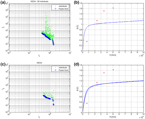
In Figure 12(b), some B–H curves estimated using solutions on Pareto front are visualized for the case in Figure 12(a), whereas Figure 12(d) shows some B–H curves for the case in Figure 12(c). The dots in Figure 12(b) and (d) represent the measured points of the B–H curve of a magnetic material.

Figure 13(a) reports the approximated Pareto front obtained using the MNSGA-1 algorithm and Figure 13(c) the one obtained using the MNSGA-2 algorithm setting the population to N_p = 20 and the number of generations to N_g = 50. In Figure 13(b), some B–H curves estimated using solutions on Pareto front are visualized for the case in Figure 13(a), whereas Figure 13(d) shows some B–H curves for the case in Figure 13(c). The dots in Figure 13(b) and (d) represent the measured points of the B–H curve of a magnetic material.

Figure 13. The approximated Pareto front using (a) MNSGA-1 and (c) MNSGA-2. Algorithms setting N_p = 20, N_g = 50, N_m = 10 and T_m = 5. (b) and (d) are the B–H curves estimated using design variables of solutions in the Pareto set.

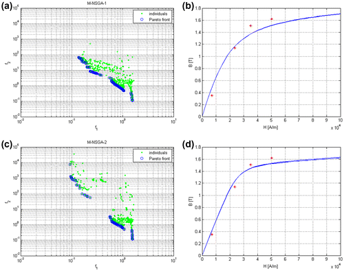
Figure 13 shows that the migration strategy expands the estimated Pareto front and the estimated B–H curves are closer to measured values. The migration parameters have been set to N_m = 10 and T_m = 5. Also in this case, the estimated B–H curves are close to measured value.

Finally, Figure 14(a) shows the approximated Pareto front obtained using the MNSGA-1 algorithm and Figure 14(c) the one obtained using the MNSGA-2 algorithm setting the population numerosity to N_p = 20 and the number of generations to Ng = 20. In this case, the migration parameters have been set to N_m = 10 and T_m = 2.

Figure 14. (a) The approximated Pareto front using (a) MNSGA-1 and (c) MNSGA-2. Algorithms setting N_p = 20, N_g = 20, N_m = 10 and T_m = 2. (b) and (d) are the B–H curves estimated using design variables of solutions in the Pareto set.

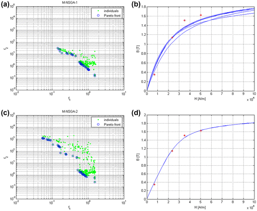
In Figure 14(b), some B–H curves estimated using solutions on Pareto front are visualized for the case in Figure 14(a), whereas Figure 14(d) shows some B–H curves for the case in Figure 14(c). The dots in Figure 14(b) and (d) represent the measured points of the B–H curve of a magnetic material.

Both the migration strategies applied to enhance NSGA algorithm in non-elitist search have shown to be effective also for this case study, making the Pareto front broader and so giving rise to a better identification of the B–H curve from measurement data.

Problem #3: finite element-based case study – results

Figure 15 reports the approximated Pareto fronts obtained using NSGA-II and MNSGA-1 algorithms starting from the same initial population and the same number of generations (N_g = 50) for the problem #3 based on finite elements simulations. The migration parameters of MNSGA-1 algorithm have been set to N_m = 10 and T_m = 5.

Figure 15. Approximated Pareto front using NSGA-II (circles) and MNSGA-1 (squares) algorithm starting from the same initial population (triangles) for the problem #3.

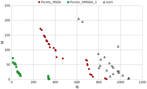
It appears that the approximation of the Pareto front obtained using MNSGA-1 is better in terms of both the objective functions used.

Conclusions

The proposed algorithm introduced a modification to a standard NSGA-II in terms of a migrating population. The new algorithm improves Pareto front estimation in problems for which the objective functions time computation does not allow the use of a large number of individuals for each generation. The proposed algorithm has been assessed by means of four test problems. Both migration strategies here developed give comparable results at the same computational cost.

Disclosure statement

No potential conflict of interest was reported by the authors.

References

- Di Barba P. Multiobjective shape design in electricity and magnetism. Doredrecht: Springer; 2010.
- Deb K. Multi-objective optimization using evolutionary algorithms. 1st ed. Chichester : Wiley; 2001.
- Neittaanmaki P, Rudnicki M, Savini A. Inverse problems and optimal design in electricity and magnetism. Oxford: Clarendon Press; 1996.
- Simon D. Biogeography-based optimization. IEEE Trans. Evol. Comput. 2008;12:702–713.10.1109/TEVC.2008.919004
- Srinivas N, Deb K. Multiobjective optimization using nondominated sorting in genetic algorithms. Evol. Comput. 1994;2:221–248.10.1162/evco.1994.2.3.221
- Deb K, Pratap A, Agarwal S, et al. A fast and elitist multiobjective genetic algorithm: NSGA-II. IEEE Trans. Evol. Comput. 2002;6:182–197.10.1109/4235.996017
- Schmitt LM. Theory of genetic algorithms. Theor. Comput. Sci. 2001;259:1–61.10.1016/S0304-3975(00)00406-0
- Di Barba P, Dolezel I, Karban P, et al. Multiphysics field analysis and multiobjective design optimization: a benchmark problem. Inverse Prob. Sci. Eng. 2014;22:1214–1225.10.1080/17415977.2013.860590
- Di Barba P, Dughiero F, Sieni E, et al. Coupled field synthesis in magnetic fluid hyperthermia. IEEE Trans. Magn. 2011;47:914–917.10.1109/TMAG.2010.2073453
- Di Barba PD, Dughiero F, Sieni E. Synthesizing a nanoparticle distribution in magnetic fluid hyperthermia. COMPEL: Int. J. Comput. Math. Electr. Electron. Eng. 2011;30:1507–1516.
- Xu S, Ji Z, Pham DT, Yu F. Binary Bees Algorithm – bioinspiration from the foraging mechanism of honeybees to optimize a multiobjective multidimensional assignment problem. Eng. Optim. 2011;43:1141–1159.10.1080/0305215X.2010.542812
- Dos Santos Coelho L, Alotto P. Tribes optimization algorithm applied to the Loney’s Solenoid. IEEE Trans. Magn. 2009;45:1526–1529.
- Hu X-M, Zhang J, Li Y. Orthogonal methods based ant colony search for solving continuous optimization problems. J. Comput. Sci. Technol. 2008;23:2–18.10.1007/s11390-008-9111-5
- Palupi Rini D, Mariyam Shamsuddin S, Sophiyati Yuhaniz S. Particle swarm optimization: technique, system and challenges. Int. J. Comput. Appl. 2011;14:19–27.10.5120/ijca
- Kennedy J, Eberhart R. Particle swarm optimization. Proc. IEEE Int. Conf. Neural Networks. 1995; 4:1942–1948.
- Di Barba P. Evolutionary multiobjective optimization methods for the shape design of industrial electromagnetic devices. IEEE Trans. Magn. 2009;45:1436–1441.10.1109/TMAG.2009.2012665
- Di Barba P, Dughiero F, Sieni E. Field synthesis for the optimal treatment planning in magnetic fluid hyperthermia. Arch. Electric. Eng. 2012;61:57–67.
- Di Barba P, Forzan M, Pozza C, et al. Optimal design of a pancake inductor for induction heating: a multiphysics and multiobjective approach. Proceeding of Sixteenth Biennial IEEE Conference on Electromagnetics Field Computation; Oita; 2012.
- Campana LG, Di Barba P, Dughiero F, et al. Optimal needle positioning for electrochemotherapy: a constrained multiobjective strategy. IEEE Trans. Magn. 2013;49:2141–2144.10.1109/TMAG.2013.2241031
- Di Barba P, Dughiero F, Forzan M, et al. A paretian approach to optimal design with uncertainties: application in induction heating. IEEE Trans. Magn. 2014;50:917–920.10.1109/TMAG.2013.2280377
- Di Barba P, Forzan M, Sieni E. Multi-objective design of a power inductor: a benchmark problem of inverse induction heating. Doležel I, editor. COMPEL – Int. J. Comput. Math. Electr. Electron Eng. 2014;33:1990–2005.
- Karakostas S. Multi-objective optimization in spatial planning: Improving the effectiveness of multi-objective evolutionary algorithms (non-dominated sorting genetic algorithm II). Eng. Optim. 2015;47:601–621.
- Ghiasi H, Pasini D, Lessard L. A non-dominated sorting hybrid algorithm for multi–objective optimization of engineering problems. Eng. Optim. 2011;43:39–59.10.1080/03052151003739598
- Di Barba P, Pleshivtseva Y, Rapoport E, et al. Multi–objective optimisation of induction heating processes: methods of the problem solution and examples based on benchmark model. Int. J. Microstruct. Mater. Prop. 2013;8:357–372.10.1504/IJMMP.2013.057072
- Pleshivtseva Y, Di Barba P, Rapoport E, et al. Multi-objective optimisation of induction heaters design based on numerical coupled field analysis. Int. J. Microstruct. Mater. Prop. 2014;9:532–551.10.1504/IJMMP.2014.067318
- Märtens M, Izzo D. The asynchronous island model and NSGA-II: study of a new migration operator and its performance. Proceedings of the 15th annual conference on genetic and evolutionary computation. Amsterdam: ACM; 2013. p. 1173–1180.
- Dos Santos Coelho L, Alotto P. Electromagnetic optimization using a cultural self-organizing migrating algorithm approach based on normative knowledge. IEEE Trans. Magn. 2009;45:1446–1449.
- Zelinka I. Real-time deterministic chaos control by means of selected evolutionary techniques. Eng. Appl. Artif. Intell. 2009;22:283–297.
- Deep K, Dipti. A self-organizing migrating genetic algorithm for constrained optimization. Appl. Math. Comput. 2008;198:237–250.10.1016/j.amc.2007.08.032
- Cocco Mariani V, Coelho LS. Global optimization of thermal conductivity using stochastic algorithms. Inverse Prob. Sci. Eng. 2009;17:511–535.
- Zelinka I. SOMA – Self-Organizing Migrating Algorithm. New optimization techniques in engineering [Internet]. Berlin: Springer; 2004. p. 167–217. Available from: http://dx.doi.org/10.1007/978-3-540-39930-8_7
- Fulginei F, Salvini A. The flock of starlings optimization: influence of topological rules on the collective behavior of swarm intelligence. In: Wiak S, Napieralska-Juszczak E, editors. Computational methods for the innovative design of electrical devices [Internet]. Berlin: Springer; 2011. p. 129–145. Available from: http://dx.doi.org/10.1007/978-3-642-16225-1_7
- Nourbakhsh A, Safikhani H, Derakhshan S. The comparison of multi-objective particle swarm optimization and NSGA II algorithm: applications in centrifugal pumps. Eng. Optim. 2011;43:1095–1113.10.1080/0305215X.2010.542811
- Koyuncu H, Ceylan R. Scout particle swarm optimization. In: Lacković I, Vasic D, editors. 6th European conference of the international federation for medical and biological engineering [Internet]. Springer International; 2015. p. 82–85. Available from: http://dx.doi.org/10.1007/978-3-319-11128-5_21
- Bertani R, Ceretta F, Di Barba P, et al. Optimal inductor design for nanofluid heating characterisation. Eng. Comput. in press.
- Di Barba P, Dughiero F, Forzan M, et al. Sensitivity-based optimal shape design of induction-heating devices. IET Sci. Meas. Technol. 2015; IET Digital Library. Available from: http://digital-library.theiet.org/content/journals/10.1049/iet-smt.2014.0227
- Roy PK, Ghoshal SP, Thakur SS. Multi-objective optimal power flow using biogeography-based optimization. Electr. Power Compon. Syst. 2010;38:1406–1426.10.1080/15325001003735176
- Singh S, Mittal E, Sachdeva G. NSBBO for gain-impedance optimization of Yagi-Uda antenna design, 2012 World Congress on information and communication technologies (WICT); 2012;p. 856–860.
- Singh U, Kumar H, Kamal TS. Design of Yagi-Uda antenna using biogeography based optimization. IEEE Trans. Antennas Propag. 2010;58:3375–3379.10.1109/TAP.2010.2055778
- Forrest S. Genetic algorithms: principles of natural selection applied to computation. Science. 1993;261:872–878.10.1126/science.8346439
- Zhang Q, Zhou A, Zhao S, et al. Multiobjective optimization test instances for the CEC 2009 special session and competition [Internet]. 2009. Available from: http://dces.essex.ac.uk/staff/zhang/MOEAcompetition/cec09testproblem0904.pdf
- Di Barba P, Komeza K, Juszczak EN, et al. Automated B–H curve identification algorithm combining field simulation with optimisation methods and exploiting parallel computation. Sci. Meas. Technol., IET. 2012;6:369–375.
- Canova A, Dughiero F, Fasolo F, et al. Identification of equivalent material properties for 3-D numerical modeling of induction heating of ferromagnetic workpieces. IEEE Trans. Magn. 2009;45:1851–1854.10.1109/TMAG.2009.2012830
- Canova A, Dughiero F, Fasolo F, et al. Simplified approach for 3-D nonlinear induction heating problems. IEEE Trans. Magn. 2009;45:1855–1858.10.1109/TMAG.2009.2012831
- FLUX. (CEDRAT). Available from: www.cedrat.com/software/flux/flux.html
- Di Barba P, Savini A, Wiak S. Field models in electricity and magnetism. Dordrecht: Springer; 2008.
- Binns KJ, Lawrenson PJ, Trowbridge CW. The analytical and numerical solution of electric and magnetic fields. Chichester: Wiley; 1992.
- Knowles, J, Thiele L, Zitzler EA. Tutorial on the performance assessment of stochastic multiobjective optimizers. Computer Engineering and Networks Laboratory; Zurich; 2006. ( Report No. TIK Report 214.)
- Zitzler E, Knowles J, Thiele L. Quality assessment of Pareto set approximations. In: Branke J, Deb K, Miettinen K, Słowiński R, editors. Multiobjective optimization [Internet]. Berlin:Springer. 2008 [cited 2015 Jan 26]. p. 373–404. Available from: http://link.springer.com/10.1007/978-3-540-88908-3_14
- Fonseca CM, Fleming PJ. On the performance assessment and comparison of stochastic multiobjective optimizers. In: Voigt H-M, Ebeling W, Rechenberg I, Schwefel H-P, editors. Parallel problem solving from nature – PPSN IV [Internet]. Berlin: Springer. 1996 [cited 2015 Jan 26]. p. 584–593. Available from: http://link.springer.com/10.1007/3-540-61723-X_1022