Inverse design of anti-reflection coatings using the nonlinear approximate inverse

Abstract

We consider a multi-frequency inverse scattering problem arising in the design of anti-reflection coatings. These thin films are deposited onto photovoltaic solar cells to enhance their performance. The objective is to determine the space-dependent refractive index in an inhomogeneous optical layer from the reflection coefficients at the surface. The relevant model yields a boundary value problem for the one-dimensional (1D) Helmholtz equation, which we formulate as an equivalent integral equation. The resulting inverse problem is nonlinear and ill-posed. We consider a series expansion of the field depending on the order of nonlinearity of the model. The first-order solution is obtained by using the Born approximation which is valid for weak scattering. Stronger scatterers are sought by considering a nonlinearity of higher order. The mathematical and numerical framework is provided by the (noniterative) method of the approximate inverse (AI) for nonlinear inverse problems. Numerical results are presented to attest the efficiency and stability of the method.

Keywords:

• Anti-reflection coating (ARC)
• Helmholtz equation
• refractive index
• nonlinear inverse problems
• regularization method

1. Introduction

Controlling the sunlight penetrating through a solar cell is essential for an optimal functioning of these semi-conductors. More than $35\%$ of the incident sunlight can be lost by normal installation without using Anti-reflection coatings (ARCs). To enhance the efficiency of the photovoltaics, an ARC is laid on the surface of the cell.[1,2] Depositing these thin films with appropriate refractive index onto the solar cells traps the sunlight which should remain propagating between two media with two different refractive indices. As a result, one saves the sunlight inside by minimizing or eliminating the light reflection. Besides photovoltaics, ARCs are widely used to ensure the decrease in the light reflection in various application areas including displays, telescopes, microscopes, ophthalmics and camera lenses.

An adaptive design of the constitutive properties of the ARCs provides a powerful tool to control the electromagnetic radiation, and so the electric current flowing through the photovoltaics. In contrast to the widely used direct design approach, we propose here a method based on the formulation as an inverse problem. In the direct design method, a prototype with specified optical properties of the coating is considered, and the generated electromagnetic field is investigated. The constitutive properties are calibrated until the desired effect is realized. However, the practical improvement of the coating design requires dealing with internal quantities, namely the refractive index. Dealing with such an internal quantity requires solving the inverse problem of the related mathematical model. The objective in the inverse problem is to determine the refractive index of the ARC for prescribed values of the electromagnetic field outside the medium. The input data for solving the inverse problem are the reflection coefficients on the free surface of the thin film.

ARCs, in their simplest settings, are designed for one layer with a single wavelength $\mathit{\lambda }$ at normal incidence. An approximately complete cancellation of the reflection occurs when the refractive index is equal to the geometric mean of the refractive indices of the ambient upper and lower media, namely $n_{\mathrm{A}RC}=n=\sqrt{n_0{n}_s}$ and $\mathit{\lambda }=4dn$. 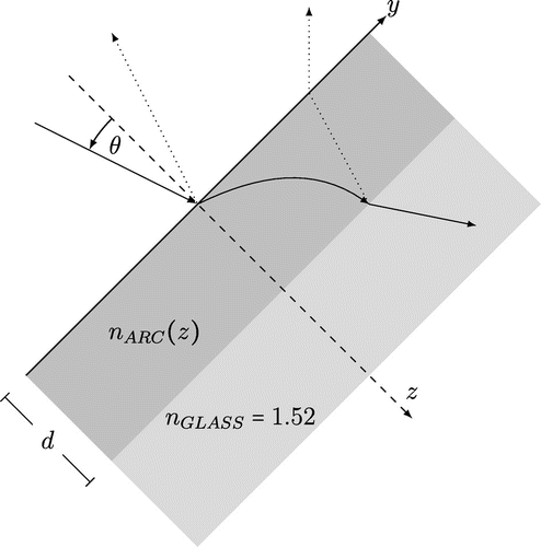The parameters $n,n_0$ and $n_{\mathrm{G}lass}=n_s$ stand for the refractive indices of the coating, free space and the glass, respectively; see Figure 1.

The parameter $d$ is the thickness of the coating. This cancellation of the reflection happens when the coating has the refractive index $n=1.23$.

However, this possibility assumes that the ARC has one constant refractive index. Moreover, it works only for one wavelength. In contrast to uni-layer films, multi-layer coatings reduce the reflections throughout a wide range of the wavelengths.[3–5] In this multi-layer setting, the coating is a stack of homogeneous layers with different constant refractive indices. Another additional setting for the ARC is to use a coating with space-dependent refractive index. A graded-index ARC with varying indices of refraction assures more absorbed energy and achieves best performance.[6,7] Therefore, we consider here a coating, which is inhomogeneous, i.e. its refractive index $n$ varies in the space.[6,8–10] Both cases, the single-layer with a constant refractive index or the multi-layer with a piece-wise constant refractive index, are special cases of our setting. For a space-dependent refractive index $n$ we may formulate the design problem as seeking an optimum $n$; for the optimization problem, we refer to [6] for this model,$$\text{minimize}\left\{||R_{\mathit{\lambda }}-(u_{\mathit{\lambda }}(n,0)-u_{\mathit{\lambda }}^0(n_0,0)){||}_{L_2({\mathit{\lambda }}_{\text{min}},{\mathit{\lambda }}_{\text{max}})},n\in \mathcal{S}\right\}$$

where $R_{\mathit{\lambda }}$ denotes the reflection coefficient at the surface, $u_{\mathit{\lambda }}^0(n_0,0)$ stands for the value of a normally incident wave at the free surface from above and $u_{\mathit{\lambda }}(n,0)$ represents the resulting wave at the free surface from below, all depending on the wavelength $\mathit{\lambda }$ in some range $[{\mathit{\lambda }}_{\text{min}},{\mathit{\lambda }}_{\text{max}}]$. The norm is taken in the space of square integrable functions $L_2.$ The set $\mathcal{S}$ denotes the class of solutions we are seeking. In our approach, we act in steps: first, we look for a solution in the set of weak scatterers, then we improve it by using a model with a higher order of nonlinearity to include stronger scattering.

We face two major difficulties when solving the inverse scattering problem. The first is the nonlinearity: the field depends on the refractive index of the object in a nonlinear manner. The second is the ill-posedness of the problem: small errors on the data result in large errors on the solution, which is typical for inverse problems.

The general existing methods to solve the inverse scattering problem depend on two approaches: using nonlinear techniques by applying iterative algorithms or using linearized inversion schemes. The nonlinear methods reconstruct the unknowns of the problem iteratively from a priori guess. These methods solve usually a sequence of forward problems using techniques such as the finite difference schemes, as done in [6], where the regularization method of Tikhonov–Phillips is used to solve the relevant nonlinear problem in the sense of least squares. As opposed to the nonlinear techniques, the linearized inversion schemes are based on approximations of Born or Rytov type, which are valid for media with low contrasts. As an application of this approximation, we refer to [9,11] for more details. Other schemes such as [12,13] solve the nonlinear inverse problem using coupled-mode Zakharov–Shabat systems. These methods are applied after a reduction of the second-order Helmholtz equation into a system of first-order differential equations. We refer also to [14] for methods based on trace formula and to [15] for methods that use spline approximation projection. For adaptive methods applied on inverse problems, we refer to e.g. [16–18]; however, we propose in this paper a completely different approach to adaptivity in inverse design.

For solving the inverse problem, we consider a method based on the physical relevance of the mathematical modelling. We start with looking for a solution in the class of weak scatterers. In this case, we may use a linearized mathematical model based on the well-known Born approximation, see [19–21]. The Born approximation is practical and feasible under some important limitations on the strength of the contrast and on the relevant range of the wave numbers. In this approximation, we assume that the scattered field is very small compared to the incident wave. Having the scattered field sufficiently small, so that it can be neglected, allows for extracting a linearized form of the problem. The shortcomings of the obtained solution, as being only valid for weak scattering, are overcome by seeking a stronger scatterer, i.e. by considering a nonlinearity of higher order. For this purpose, we use a series expansion of the field depending on the order of nonlinearity of the model. The solution to the linear problem is ameliorated using a correction derived from the quadratic model. For determining the correction term, we consider two approaches: global and local corrections. The better results are obtained using local corrections. We call the introduced procedure adaptive (inverse) modelling. The proposed method of adaptive inverse design is also applicable to nonlinear problems in higher dimensions. For the reconstruction of the refractive index of ARCs, the one-dimensional model (1D) is, however, sufficient.

The ill-posedness of the inverse problem is twofold. This is due to nonuniqueness and ill-conditioning. The application of a regularization method is then required to stabilize the solution.[22–24] We refer to [25] and [26] for a general analytical study on the regularization of ill-posed problems.

The method of the approximate inverse (AI) is a stable and flexible regularization scheme. This method, introduced by Louis and Maass [27], analysed and improved an efficient implementation using invariances by Louis [28], is used as a main regularization method in this work. It is an efficient method for solving linear [26] and nonlinear problems.[28,29]

Louis [28] extended the previously mentioned method for solving nonlinear inverse problems. We apply this method on our inverse scattering problem. Moreover, we introduce the efficient concept of adaptive inverse modelling in the framework of the AI. We use a threshold to decide locally where to apply a higher (quadratic) order of approximation. We take, here, advantage of the method of the AI as a local method.

Figure 1. ARC in contact with a glass substrate.

We outline the content of this paper as follows: In Section 2, we describe the mathematical model and derive an equivalent integral equation of Lippmann–Schwinger type. In Section 3, we are concerned with the formulation of the inverse nonlinear problem which is linearized using the iterated Born approximation. The application of the method of the AI on the linearized problem is discussed in Section 4. The nonlinear problem is treated in Section 5.1. In the last section, we present some numerical simulations.

2. Mathematical formulation of the direct problem

Let a plane wave in the time-harmonic regime be propagating through a stratified nonmagnetic medium with a constant magnetic permeability ${\mathit{\mu }}_0=1$ and a dielectric permittivity $\mathit{\epsilon }=\mathit{\epsilon }(z)$, where $z$ is the direction of stratification and of incidence. We consider the case of a normal incidence, i.e. the incident angle $\mathit{\theta }=0$, see Figure 1. We suppose the electric wave $\mathbf{E}=(E_x,E_y,E_z)$ to be linearly polarized in the direction perpendicular to the plane of incidence, i.e. a transverse electric wave (denoted by TE). For a TE wave, the polarization is along the $x$-direction, this means $E_y=E_z=0$. The time-harmonic Maxwell’s equations relate the electric field $\mathbf{E}$ and the magnetic field $\mathbf{H}$ to the constitutive properties of the meduim $\mathit{\epsilon }$, see e.g. [19],(2.1) $$\begin{array}{cc}\hfill \mathrm{\nabla }\times \mathbf{E}-i\mathit{\omega }{\mathit{\mu }}_0\mathbf{H}& =0,\hfill \\ \hfill \mathrm{\nabla }\times \mathbf{H}+i\mathit{\omega }\mathit{\epsilon }(z)\mathbf{E}& =0.\hfill \end{array}$$(2.1)

where $\mathrm{\nabla }={({\mathit{\partial }}_x,{\mathit{\partial }}_y,{\mathit{\partial }}_z)}^T$ denotes the Nabla operator and $\times$ is the cross product. In the framework of ARC, we consider a normally incident wave $E_x^{\text{inc}}=u^{\text{inc}}(z)=e^{i\mathit{\kappa }{n}_{0}z}$, where $n_0$ is the refractive index of the air environment ($n_0=1$). The ARC has a given thickness $d$ and a refractive index $n_{\text{ARC}}(z)=n(z)$, in contact with a glass substrate of uniform refractive index $n_{\text{Glass}}=n_s=1.52$. Let the interval $\mathrm{\Omega }=(0,d)\in \mathbb{R}$ be the bounded domain of the relevant coating with the points $z=0$ and $z=d$ as the ARC boundaries. For the sake of scaling into the interval $[0,1]$, we replace $z$ with $z/d$ and set $\mathit{\beta }=\mathit{\kappa }d$ as the nondimensionalized wave number. We define the contrast function $f:=n^2-1$ between the ARC and the air. It yields a boundary value problem (BVP) for the Helmholtz equation in one dimension [6,9](2.2) $$\begin{array}{c}\hfill (\text{BVP})\left\{\begin{array}{cc}\hfill u^{″}(z)+{\mathit{\beta }}^{2}u(z)=& -{\mathit{\beta }}^{2}f(z)u(z),z\in (0,1),\\ \hfill u^{\prime }(0)+i{n}_0\mathit{\beta }u(0)=& 2i{n}_0\mathit{\beta },\\ \hfill u^{\prime }(1)-i{n}_s\mathit{\beta }u(1)=& 0.\end{array}\right.\end{array}$$(2.2)

where $u$ is the resulting (or total) field, $u^{\prime }$ denotes the first derivative and $u^{″}$ is the second derivative of $u.$

For solving the boundary value problem defined in (2.3(2.3) $$\begin{array}{c}\hfill u^{″}(z)+{\mathit{\beta }}^{2}u(z)=-{\mathit{\beta }}^{2}f(z)u(z).\end{array}$$(2.3) ), we formulate it as an equivalent integral equation. We recall the model equation as(2.3) $$\begin{array}{c}\hfill u^{″}(z)+{\mathit{\beta }}^{2}u(z)=-{\mathit{\beta }}^{2}f(z)u(z).\end{array}$$(2.3)

We split the total solution of Equation (2.4(2.4) $$\begin{array}{c}\hfill u(z)=u^0(z)+u^s(z),\end{array}$$(2.4) ) into a sum of an incident wave and a scattered wave(2.4) $$\begin{array}{c}\hfill u(z)=u^0(z)+u^s(z),\end{array}$$(2.4)

where(2.5) $$\begin{array}{c}\hfill u^0(z)=e^{i\mathit{\beta }z}+\mathit{\eta }{e}^{-i\mathit{\beta }(z-2)},\end{array}$$(2.5)

with $\mathit{\eta }:=\frac{1-n_s}{1+n_s}.$ The function $u^0$ is a solution of the homogeneous Helmholtz equation(2.6) $$\begin{array}{c}\hfill u^{″}(z)+{\mathit{\beta }}^{2}u(z)=0.\end{array}$$(2.6)

satisfying the boundary conditions in (2.3(2.3) $$\begin{array}{c}\hfill u^{″}(z)+{\mathit{\beta }}^{2}u(z)=-{\mathit{\beta }}^{2}f(z)u(z).\end{array}$$(2.3) ). The solution $u^s$ of the inhomogeneous Helmholtz equation (2.4(2.4) $$\begin{array}{c}\hfill u(z)=u^0(z)+u^s(z),\end{array}$$(2.4) ) is given as(2.7) $$\begin{array}{c}\hfill {\displaystyle u^s(z)=-{\mathit{\beta }}^2{\int }_0^1{k}_{\mathit{\beta }}(z,\mathit{\tau })u(\mathit{\tau })f(\mathit{\tau })\mathrm{d}\mathit{\tau },}\end{array}$$(2.7)

where we determine $k_{\mathit{\beta }}$ using the boundary conditions in (2.3(2.3) $$\begin{array}{c}\hfill u^{″}(z)+{\mathit{\beta }}^{2}u(z)=-{\mathit{\beta }}^{2}f(z)u(z).\end{array}$$(2.3) ). Let $k_1$ be a solution to(2.8) $$\begin{array}{cc}\hfill k_1^{″}+{\mathit{\beta }}^2{k}_1& =0,\hfill \\ \hfill k_1^{\prime }(0)+i{n}_0\mathit{\beta }{k}_1(0)& =0\hfill \end{array}$$(2.8)

and $k_2$ be a solution to(2.9) $$\begin{array}{cc}\hfill k_2^{″}+{\mathit{\beta }}^2{k}_2& =0,\hfill \\ \hfill k_2^{\prime }(1)-i{n}_s\mathit{\beta }{k}_2(1)& =0\hfill \end{array}$$(2.9)

We notice that $k_1$ and $k_2$ are defined up to a constant factor.

The integral kernel $k_{\mathit{\beta }}(z,\mathit{\tau })$ is obtained from the BVP (2.3(2.3) $$\begin{array}{c}\hfill u^{″}(z)+{\mathit{\beta }}^{2}u(z)=-{\mathit{\beta }}^{2}f(z)u(z).\end{array}$$(2.3) ) as(2.10) $$\begin{array}{c}\hfill k_{\mathit{\beta }}(z,\mathit{\tau })=c\left\{\begin{array}{ccc}\hfill k_1(z)k_2(\mathit{\tau })& \text{for}& z<\mathit{\tau },\hfill \\ \hfill [12pt]k_2(z)k_1(\mathit{\tau })& \text{for}& z>\mathit{\tau }\hfill \end{array}\right.\end{array}$$(2.10)

with$$\begin{array}{c}\hfill c=\frac{\mathit{\eta }{e}^{2i\mathit{\beta }}}{2i\mathit{\beta }}.\end{array}$$

A straightforward computation yields(2.11) $$\begin{array}{c}\hfill k_{\mathit{\beta }}(z,\mathit{\tau })=\left\{\begin{array}{ccc}\hfill \frac{1}{2i\mathit{\beta }}{e}^{-i\mathit{\beta }(z-\mathit{\tau })}+\frac{\mathit{\eta }}{2i\mathit{\beta }}{e}^{-i\mathit{\beta }(z+\mathit{\tau }-2)}& \text{for}& z\le \mathit{\tau },\hfill \\ \hfill [12pt]\frac{1}{2i\mathit{\beta }}{e}^{+i\mathit{\beta }(z-\mathit{\tau })}+\frac{\mathit{\eta }}{2i\mathit{\beta }}{e}^{-i\mathit{\beta }(z+\mathit{\tau }-2)}& \text{for}& z>\mathit{\tau }.\hfill \end{array}\right.\end{array}$$(2.11)

If we substitute (2.6(2.6) $$\begin{array}{c}\hfill u^{″}(z)+{\mathit{\beta }}^{2}u(z)=0.\end{array}$$(2.6) ) and (2.8(2.8) $$\begin{array}{cc}\hfill k_1^{″}+{\mathit{\beta }}^2{k}_1& =0,\hfill \\ \hfill k_1^{\prime }(0)+i{n}_0\mathit{\beta }{k}_1(0)& =0\hfill \end{array}$$(2.8) ) in Equation (2.5(2.5) $$\begin{array}{c}\hfill u^0(z)=e^{i\mathit{\beta }z}+\mathit{\eta }{e}^{-i\mathit{\beta }(z-2)},\end{array}$$(2.5) ), we obtain the total solution as(2.12) $$\begin{array}{c}\hfill {\displaystyle u(\mathit{\beta },z)=u^0(\mathit{\beta },z)-{\int }_0^1{\mathit{\beta }}^2{k}_{\mathit{\beta }}(z,\mathit{\tau })f(\mathit{\tau })u(\mathit{\beta },y)\mathrm{d}\mathit{\tau }.}\end{array}$$(2.12)

For a given contrast function $f$ of the coating, we get a Fredholm equation of the second kind with respect to the field $u$(2.13) $$\begin{array}{c}\hfill {\displaystyle u(\mathit{\beta },z)+{\int }_0^1{k}^f(\mathit{\beta },z,\mathit{\tau })u(\mathit{\beta },\mathit{\tau })\mathrm{d}\mathit{\tau }=u^0(\mathit{\beta },z),z\in (0,1),}\end{array}$$(2.13)

with the kernel$$\begin{array}{c}\hfill k^f(\mathit{\beta },z,\mathit{\tau })={\mathit{\beta }}^2{k}_{\mathit{\beta }}(z,\mathit{\tau })f(\mathit{\tau }).\end{array}$$

Equation (2.16(3.3) $$\begin{array}{c}\hfill u=u^0+Afu,\end{array}$$(3.3) ) is known in the scattering theory as Lippmann–Schwinger integral equation.[19,30] Thus, the direct problem is concerned with the determination of the total field $u$ from a given incident field $u^0$ and a given refractive index $n$,  i.e. contrast function $f=n^2-1$.

3. The nonlinear inverse scattering problem

The inverse problem considered in this article is concerned with the determination of the refractive indices of the optical coating based on the values of the reflection coefficients which represent the input data.

These data are given for different values of the wave numbers. If we consider the integral formulation (2.15(3.2) $$\begin{array}{c}\hfill {\displaystyle -{\int }_0^1{\mathit{\beta }}^2{k}_{\mathit{\beta }}(0,y)u(y,\mathit{\beta })f(y)\mathrm{d}y=\underset{\text{Data}=:g(\mathit{\beta })}{\underbrace{u(0,\mathit{\beta })-u^0(0,\mathit{\beta })}},}\end{array}$$(3.2) ), we obtain the total field as(3.1) $$\begin{array}{c}\hfill {\displaystyle u(x,\mathit{\beta })=u^0(x,\mathit{\beta })-{\mathit{\beta }}^2{\int }_0^1{k}_{\mathit{\beta }}(x,y)u(y,\mathit{\beta })f(y)\mathrm{d}y\text{for}x\in [0,1].}\end{array}$$(3.1)

The reflection coefficient at the surface determines the value of the field $u$ at $x=0.$ We refer to [9] for more details. We get(3.2) $$\begin{array}{c}\hfill {\displaystyle -{\int }_0^1{\mathit{\beta }}^2{k}_{\mathit{\beta }}(0,y)u(y,\mathit{\beta })f(y)\mathrm{d}y=\underset{\text{Data}=:g(\mathit{\beta })}{\underbrace{u(0,\mathit{\beta })-u^0(0,\mathit{\beta })}},}\end{array}$$(3.2)

which is an integral equation of the first kind. The kernel $k_{\mathit{\beta }}(0,y)$ is obtained from (2.14(3.1) $$\begin{array}{c}\hfill {\displaystyle u(x,\mathit{\beta })=u^0(x,\mathit{\beta })-{\mathit{\beta }}^2{\int }_0^1{k}_{\mathit{\beta }}(x,y)u(y,\mathit{\beta })f(y)\mathrm{d}y\text{for}x\in [0,1].}\end{array}$$(3.1) ) as$$\begin{array}{c}\hfill k_{\mathit{\beta }}(0,y)=\frac{1}{2i\mathit{\beta }}(e^{i\mathit{\beta }y}+\mathit{\eta }{e}^{-i\mathit{\beta }y}{e}^{2i\mathit{\beta }}).\end{array}$$

For a given field $u$, we have to find the unknown contrast function $f$, i.e. the refractive index $n^2=1+f$. This optical coating synthesis problem is an inverse medium scattering problem. Inverse scattering problems arise when information about some unknown object are recovered depending on measurements of waves scattered by this object. Such problems arise in diverse areas of applications as medical diagnostics, nondestructive industrial testing, submarines and oil exploration. For more details about inverse scattering problems, we refer to [30]. One of the main difficulties in solving the inverse scattering problems is the nonlinear dependence of the field $u$ on the contrast function $f$. In the literature, we can classify the methods of solution into two types. The first one uses nonlinear techniques by applying e.g. iterative algorithms, whereas the second approach treats linearized inversion schemes. The linearized schemes depend on approximations of Born or Rytov type [20,21] which are valid for media with low contrasts, e.g. [11]. We use the Born approximation for linearizing the mathematical integral model (3.1(3.1) $$\begin{array}{c}\hfill {\displaystyle u(x,\mathit{\beta })=u^0(x,\mathit{\beta })-{\mathit{\beta }}^2{\int }_0^1{k}_{\mathit{\beta }}(x,y)u(y,\mathit{\beta })f(y)\mathrm{d}y\text{for}x\in [0,1].}\end{array}$$(3.1) ). We refer to [19,20] for more details about the Born approximation.

We consider the integral formulation (3.1(3.1) $$\begin{array}{c}\hfill {\displaystyle u(x,\mathit{\beta })=u^0(x,\mathit{\beta })-{\mathit{\beta }}^2{\int }_0^1{k}_{\mathit{\beta }}(x,y)u(y,\mathit{\beta })f(y)\mathrm{d}y\text{for}x\in [0,1].}\end{array}$$(3.1) ). In operator notation, it reads(3.3) $$\begin{array}{c}\hfill u=u^0+Afu,\end{array}$$(3.3)

where $A$ is the linear operator given ($\text{with}\mathit{\phi }=fu$) as(3.4) $$\begin{array}{c}\hfill {\displaystyle A\mathit{\phi }(x,\mathit{\beta })=-{\int }_0^1{\mathit{\beta }}^2{k}_{\mathit{\beta }}(x,y)\mathit{\phi }(y)\mathrm{d}y.}\end{array}$$(3.4)

We denote by $\mathcal{I}$ the identity operator and $A_f$ the operator defined as $A_{f}u=Afu$. Equation (3.3(3.3) $$\begin{array}{c}\hfill u=u^0+Afu,\end{array}$$(3.3) ) reads as(3.5) $$\begin{array}{c}\hfill u={(\mathcal{I}-A_f)}^{-1}{u}^0,\end{array}$$(3.5)

The operator $(\mathcal{I}-A_f)$ is supposed to be invertible in the vicinity of $f_0=0$ and ${(\mathcal{I}-A_f)}^{-1}$ which denotes the inverse operator of $(\mathcal{I}-A_f)$. From (3.5(3.5) $$\begin{array}{c}\hfill u={(\mathcal{I}-A_f)}^{-1}{u}^0,\end{array}$$(3.5) ), we get the infinite Born series for the field $u$(3.6) $$\begin{array}{c}\hfill u=\sum _{l=0}^{\infty }{(A_f)}^l{u}^0.\end{array}$$(3.6)

Thus, the Born series is a Taylor expansion of (3.3(3.3) $$\begin{array}{c}\hfill u=u^0+Afu,\end{array}$$(3.3) ) at $f_0=0$.

The terms of this series represent the successively higher orders of the scattering.[19] If we just consider the first two orders in (3.6(3.6) $$\begin{array}{c}\hfill u=\sum _{l=0}^{\infty }{(A_f)}^l{u}^0.\end{array}$$(3.6) ) and ignore the other higher orders, we obtain the finite Born series up to a second order as(3.7) $$\begin{array}{c}\hfill u(x,\mathit{\beta })\approx \underset{l=0}{\underbrace{u^0(x,\mathit{\beta })}}+\underset{l=1}{\underbrace{A_f[u^0(y,\mathit{\beta })]}}+\underset{l=2}{\underbrace{A_f[A_f[u^0(y,\mathit{\beta })]]}},\end{array}$$(3.7)

here $l=1$ and $l=2$ stand for the Born approximation for the field $u$ of the first order and of the second order, respectively. The electric field is measured at the point $x=0$ and substituted in (3.7(3.7) $$\begin{array}{c}\hfill u(x,\mathit{\beta })\approx \underset{l=0}{\underbrace{u^0(x,\mathit{\beta })}}+\underset{l=1}{\underbrace{A_f[u^0(y,\mathit{\beta })]}}+\underset{l=2}{\underbrace{A_f[A_f[u^0(y,\mathit{\beta })]]}},\end{array}$$(3.7) ) to obtain the equation(3.8) $$\begin{array}{c}\hfill \underset{\text{linear}(A_1)}{\underbrace{A_f[u^0(·,\mathit{\beta })](\mathit{\beta })}}+\underset{\text{quadratic}(A_2)}{\underbrace{A_f[A_f[u^0(·,\mathit{\beta })]](\mathit{\beta })}}=\underset{=g(\mathit{\beta })\text{(Data)}}{\underbrace{u(0,\mathit{\beta })-u^0(0,\mathit{\beta })}}.\end{array}$$(3.8)

4. Application of the linear AI

Here, we are concerned with the case $l=1$ in (3.7(3.7) $$\begin{array}{c}\hfill u(x,\mathit{\beta })\approx \underset{l=0}{\underbrace{u^0(x,\mathit{\beta })}}+\underset{l=1}{\underbrace{A_f[u^0(y,\mathit{\beta })]}}+\underset{l=2}{\underbrace{A_f[A_f[u^0(y,\mathit{\beta })]]}},\end{array}$$(3.7) ). Thus, we linearize the problem using the first-order Born approximation. The scattered field $u^s$ is supposed to be much smaller than the incident field $u^0$. Therefore, it could be neglected in (2.5(2.5) $$\begin{array}{c}\hfill u^0(z)=e^{i\mathit{\beta }z}+\mathit{\eta }{e}^{-i\mathit{\beta }(z-2)},\end{array}$$(2.5) ) by setting(4.1) $$\begin{array}{c}\hfill u(y,\mathit{\beta })\approx u^0(y,\mathit{\beta })\text{for}y\in (0,1).\end{array}$$(4.1)

By substituting (4.1(4.1) $$\begin{array}{c}\hfill u(y,\mathit{\beta })\approx u^0(y,\mathit{\beta })\text{for}y\in (0,1).\end{array}$$(4.1) ) in the left-hand side of (3.2(3.2) $$\begin{array}{c}\hfill {\displaystyle -{\int }_0^1{\mathit{\beta }}^2{k}_{\mathit{\beta }}(0,y)u(y,\mathit{\beta })f(y)\mathrm{d}y=\underset{\text{Data}=:g(\mathit{\beta })}{\underbrace{u(0,\mathit{\beta })-u^0(0,\mathit{\beta })}},}\end{array}$$(3.2) ), we obtain the linear Fredholm integral equation of the first kind(4.2) $$\begin{array}{c}\hfill {\displaystyle -{\int }_0^1\underset{=:\tilde{k}(\mathit{\beta },y)}{\underbrace{{\mathit{\beta }}^2{k}_{\mathit{\beta }}(0,y)u^0(y,\mathit{\beta })}}f(y)\mathrm{d}y=\underset{=:g(\mathit{\beta })}{\underbrace{u(0,\mathit{\beta })-u^0(0,\mathit{\beta })}}.}\end{array}$$(4.2)

Let $A_1$ be the operator(4.3) $$\begin{array}{c}\hfill A_1:X=L_2([0,1])⟶L_2([{\mathit{\beta }}_{\min },{\mathit{\beta }}_{\max }])=Y,\\ \hfill {\displaystyle A_{1}f(\mathit{\beta })={\int }_0^1\tilde{k}(\mathit{\beta },y)f(y)\mathrm{d}y}\end{array}$$(4.3)

where $A_1$ is the linearized operator and $\tilde{k}(\mathit{\beta },y)$ is the integral kernel given by(4.4) $$\begin{array}{c}\hfill \tilde{k}(\mathit{\beta },y)=\frac{\mathit{\beta }i}{2}\left(e^{2i\mathit{\beta }y}+{\mathit{\eta }}^2{e}^{-2i\mathit{\beta }(y-2)}+2\mathit{\eta }{e}^{2i\mathit{\beta }}\right).\end{array}$$(4.4)

The data are the differences between the values of the total and incident fields at the point $x=0$. These differences are called the reflection coefficients. From these data, we have to find the unknown contrast function $f,$ i.e. the refractive index $n=\sqrt{1+f}$. To numerically solve this inverse problem, we seek a system of linear equations. This requires a diversity of the wave number $\mathit{\beta }$. The nondimensionalized wave number $\mathit{\beta }$ is ranging in the interval $\left[{\mathit{\beta }}_{\mathrm{m}in},{\mathit{\beta }}_{\mathrm{m}ax}\right]$. Hence, our linearized semi-discrete problem seeks $f$ as a solution of the equation:(4.5) $$\begin{array}{c}\hfill A_{1}f({\mathit{\beta }}_j)=g({\mathit{\beta }}_j)j=1,\dots ,M,\end{array}$$(4.5)

where ${\mathit{\beta }}_j$ are samplings of the wave numbers. The Born approximation is valid for a contrast function $f$ satisfying the inequality(4.6) $$\begin{array}{c}\hfill \mathit{\kappa }d\underset{x\in (0,1)}{sup}\left|f(x)\right|<c,\end{array}$$(4.6)

where $c=4\mathit{\pi }b$ with $b$ a small constant; in practice, we take $b=0.16$, see, e.g. [21]. The left-hand side of this inequality is a rough estimate for the phase shift between the incident field and the wave propagation throughout the object. The range of the wave numbers $[{\mathit{\beta }}_{\min },{\mathit{\beta }}_{\max }]$ taken in the numerical test examples must satisfy the condition above in order to get a good reconstruction.

4.1. The AI for linear problems

As an efficient and stable regularization scheme, we apply the method of the AI to stabilize the solution of our linearized problem (4.3(4.3) $$\begin{array}{c}\hfill A_1:X=L_2([0,1])⟶L_2([{\mathit{\beta }}_{\min },{\mathit{\beta }}_{\max }])=Y,\\ \hfill {\displaystyle A_{1}f(\mathit{\beta })={\int }_0^1\tilde{k}(\mathit{\beta },y)f(y)\mathrm{d}y}\end{array}$$(4.3) ). This method was firstly introduced in [27]. For the analytic study and efficient implementation of this regularization method, we refer to Louis [28]. The AI is an efficient method for solving linear [26] and nonlinear problems.[28,29] It has been extended for image reconstruction,[31] for feature reconstruction[32] and for solving inverse problems on Banach spaces.[33,34] This method has been implemented successfully in many applications.[22,35]

We consider a compact linear operator $A$ between the Hilbert space $X$ and $Y$ endowed with the scalar products ${〈\mathrm{cdot},\mathrm{cdot}〉}_X$ and ${〈·,·〉}_X$. The aim of this method is to find a stable solution $f$ to an ill-posed equation $Af=g$ by computing an approximation$$\begin{array}{cc}\hfill f_{\mathit{\gamma }}(x)& ={〈f,{\mathit{\delta }}_x^{\mathit{\gamma }}〉}_X\text{with}{\mathit{\delta }}_x^{\mathit{\gamma }}\approx {\mathit{\delta }}_x.\hfill \end{array}$$

The mollifier ${\mathit{\delta }}_x^{\mathit{\gamma }}$ converges (as $\mathit{\gamma }$ tends to zero) to the delta distribution ${\mathit{\delta }}_x$ for the reconstruction point $x$. A typical example is the Gaussian mollifier given by(4.7) $$\begin{array}{c}\hfill {\mathit{\delta }}_x^{\mathit{\gamma }}(y)={(2\mathit{\pi })}^{-n/2}{\mathit{\gamma }}^{-n}exp\left(-{\mid x-y\mid }^2\left(2{\mathit{\gamma }}^2\right)\right)\end{array}$$(4.7)

The parameter $\mathit{\gamma }$ acts as a regularization parameter. To relate the data $g$ to the solution, we have to determine a reconstruction kernel ${\mathit{\psi }}_x^{\mathit{\gamma }}$ by solving the following auxiliary equation(4.8) $$\begin{array}{c}\hfill A^{\ast }{\mathit{\psi }}_x^{\mathit{\gamma }}={\mathit{\delta }}_x^{\mathit{\gamma }},\end{array}$$(4.8)

where ${\mathit{\delta }}_x^{\mathit{\gamma }}$ is the mollifier defined above and $A^{\ast }$ is the adjoint operator of $A$ satisfying ${〈Af,g〉}_Y={〈f,A^{\ast }g〉}_X$ for every $f\in X,g\in Y$. If Equation (4.8(4.8) $$\begin{array}{c}\hfill A^{\ast }{\mathit{\psi }}_x^{\mathit{\gamma }}={\mathit{\delta }}_x^{\mathit{\gamma }},\end{array}$$(4.8) ) is not solvable, then the reconstruction kernel ${\mathit{\psi }}_x^{\mathit{\gamma }}$ is approximated by minimizing the defect $\Vert A^{\ast }{\mathit{\psi }}^{\mathit{\gamma }}-{\mathit{\delta }}^{\mathit{\gamma }}\Vert$ which leads to the normal equation of (4.8(4.8) $$\begin{array}{c}\hfill A^{\ast }{\mathit{\psi }}_x^{\mathit{\gamma }}={\mathit{\delta }}_x^{\mathit{\gamma }},\end{array}$$(4.8) ) as(4.9) $$\begin{array}{c}\hfill A{A}^{\ast }{\mathit{\psi }}_x^{\mathit{\gamma }}=A{\mathit{\delta }}_x^{\mathit{\gamma }}.\end{array}$$(4.9)

Then, depending on (4.8(4.8) $$\begin{array}{c}\hfill A^{\ast }{\mathit{\psi }}_x^{\mathit{\gamma }}={\mathit{\delta }}_x^{\mathit{\gamma }},\end{array}$$(4.8) ), it holds(4.10) $$\begin{array}{cc}\hfill f_{\mathit{\gamma }}(x)& ={〈f,{\mathit{\delta }}_x^{\mathit{\gamma }}〉}_X\hfill \\ \hfill & ={〈f,A^{\ast }{\mathit{\psi }}_x^{\mathit{\gamma }}〉}_X\hfill \\ \hfill & ={〈Af,{\mathit{\psi }}_x^{\mathit{\gamma }}〉}_Y\hfill \\ \hfill & ={〈g,{\mathit{\psi }}_x^{\mathit{\gamma }}〉}_Y=:S_{\mathit{\gamma }}g(x).\hfill \end{array}$$(4.10)

For ${\mathit{\delta }}_x^{\mathit{\gamma }}$, a suitable mollifier, let ${\mathit{\psi }}_x^{\mathit{\gamma }}$ be the solution of (4.9(4.9) $$\begin{array}{c}\hfill A{A}^{\ast }{\mathit{\psi }}_x^{\mathit{\gamma }}=A{\mathit{\delta }}_x^{\mathit{\gamma }}.\end{array}$$(4.9) ). Then, $S_{\mathit{\gamma }}g:=〈g,{\mathit{\psi }}_x^{\mathit{\gamma }}〉$ is called the Approximate Inverse of the operator $A$ and ${\mathit{\psi }}_x^{\mathit{\gamma }}$ is called the reconstruction kernel.

4.2. Solution of the linearized problem

We recall now the linearized operator (4.3(4.3) $$\begin{array}{c}\hfill A_1:X=L_2([0,1])⟶L_2([{\mathit{\beta }}_{\min },{\mathit{\beta }}_{\max }])=Y,\\ \hfill {\displaystyle A_{1}f(\mathit{\beta })={\int }_0^1\tilde{k}(\mathit{\beta },y)f(y)\mathrm{d}y}\end{array}$$(4.3) ) of our model. Thus, the adjoint operator of $A_1$ is given as(4.11) $$\begin{array}{cc}\hfill A_1^{\ast }& :L_2([{\mathit{\beta }}_{\min },{\mathit{\beta }}_{\max }])⟶L_2([0,1]),\hfill \\ \hfill (A_1^{\ast }g)(y)& {\displaystyle ={\int }_{{\mathit{\beta }}_{\min }}^{{\mathit{\beta }}_{\max }}{\tilde{k}}^{\ast }(y,\mathit{\beta })g(\mathit{\beta })d\mathit{\beta },y\in [0,1].}\hfill \end{array}$$(4.11)

Applying the adjoint operator on the reconstruction kernel, we get the auxiliary equation in the following integral form(4.12) $$\begin{array}{c}\hfill {\displaystyle (A_1^{\ast }{\mathit{\psi }}_x^{\mathit{\gamma }})(y)={\int }_{{\mathit{\beta }}_{\min }}^{{\mathit{\beta }}_{\max }}{\tilde{k}}^{\ast }(y,\mathit{\beta }){\mathit{\psi }}_x^{\mathit{\gamma }}(\mathit{\beta })d\mathit{\beta }={\mathit{\delta }}_x^{\mathit{\gamma }}(y),y\in [0,1],}\end{array}$$(4.12)

where the integral kernel of $A^{\ast }$ is computed by(4.13) $$\begin{array}{c}\hfill {\tilde{k}}^{\ast }(y,\mathit{\beta })=\overline{\tilde{k}(y,\mathit{\beta })}=\frac{-\mathit{\beta }i}{2}\left(e^{-2i\mathit{\beta }y}+{\mathit{\eta }}^2{e}^{2i\mathit{\beta }(y-2)}+2\mathit{\eta }{e}^{-2i\mathit{\beta }}\right).\end{array}$$(4.13)

For determining the reconstruction kernel in (4.12(4.12) $$\begin{array}{c}\hfill {\displaystyle (A_1^{\ast }{\mathit{\psi }}_x^{\mathit{\gamma }})(y)={\int }_{{\mathit{\beta }}_{\min }}^{{\mathit{\beta }}_{\max }}{\tilde{k}}^{\ast }(y,\mathit{\beta }){\mathit{\psi }}_x^{\mathit{\gamma }}(\mathit{\beta })d\mathit{\beta }={\mathit{\delta }}_x^{\mathit{\gamma }}(y),y\in [0,1],}\end{array}$$(4.12) ), we solve the corresponding normal equation which involves the operator$$\begin{array}{c}\hfill A_1{A}_1^{\ast }:L_2([{\mathit{\beta }}_{\min },{\mathit{\beta }}_{\max }])⟶L_2([{\mathit{\beta }}_{\min },{\mathit{\beta }}_{\max }]),\end{array}$$

where(4.14) $$\begin{array}{cc}\hfill A_1{A}_1^{\ast }g(\mathit{\beta })& {\displaystyle ={\int }_0^1\tilde{k}(y,\mathit{\beta })\underset{(4.11)}{\underbrace{A_1^{\ast }g(y)}}\mathrm{d}y}\hfill \\ \hfill & {\displaystyle ={\int }_0^1\tilde{k}(y,\mathit{\beta })\left[{\displaystyle {\int }_{{\mathit{\beta }}_{\min }}^{{\mathit{\beta }}_{\mathrm{m}ax}}{\tilde{k}}^{\ast }(y,{\mathit{\beta }}^{\prime })g({\mathit{\beta }}^{\prime })\mathrm{d}{\mathit{\beta }}^{\prime }}\right]\mathrm{d}y}\hfill \\ \hfill & {\displaystyle ={\int }_{{\mathit{\beta }}_{\min }}^{{\mathit{\beta }}_{\max }}\underset{\mathbf{Gram}\mathbf{Matrix}}{\underbrace{\left[{\displaystyle {\int }_0^1\tilde{k}(y,\mathit{\beta }){\tilde{k}}^{\ast }(y,{\mathit{\beta }}^{\prime })\mathrm{d}y}\right]}}g({\mathit{\beta }}^{\prime })\mathrm{d}{\mathit{\beta }}^{\prime },\text{for}\mathit{\beta },{\mathit{\beta }}^{{}^{\prime }}\in \left[{\mathit{\beta }}_{\min },{\mathit{\beta }}_{\max }\right].}\hfill \end{array}$$(4.14)

By discretizing the interval $[{\mathit{\beta }}_{\mathrm{m}in},{\mathit{\beta }}_{\mathrm{m}ax}]$, the space $Y$ is replaced by the Euclidean space ${\mathbb{R}}^M$. Here, $M$ denotes the number of the wave lengths ${\mathit{\lambda }}_j,j=1,\dots ,M$ taken in the interval $[{\mathit{\lambda }}_{\mathrm{m}in},{\mathit{\lambda }}_{\mathrm{m}ax}]$. We take ${\mathit{\beta }}_j$ with $1\le j\le M$, such that(4.15) $$\begin{array}{c}\hfill {\mathit{\beta }}_1={\mathit{\beta }}_{\mathrm{m}in}=\frac{2\mathit{\pi }d}{{\mathit{\lambda }}_{\mathrm{m}ax}}\text{and}{\mathit{\beta }}_M={\mathit{\beta }}_{\mathrm{m}ax}=\frac{2\mathit{\pi }d}{{\mathit{\lambda }}_{\mathrm{m}in}}.\end{array}$$(4.15)

Depending on this discretization, the matrix that represents $A_1{A}_1^{\ast }$ is called the Gram matrix $G$ which is given as$$\begin{array}{c}\hfill {\displaystyle G_{\mathit{\beta }{\mathit{\beta }}^{\prime }}={\int }_0^1\tilde{k}(y,\mathit{\beta }){\tilde{k}}^{\ast }(y,{\mathit{\beta }}^{\prime })\mathrm{d}y,\text{for}\mathit{\beta },{\mathit{\beta }}^{{}^{\prime }}\in \left\{{\mathit{\beta }}_j,j=1,\dots ,M\right\}}\end{array}$$

Similar to the discrete system of equations in (4.12(4.12) $$\begin{array}{c}\hfill {\displaystyle (A_1^{\ast }{\mathit{\psi }}_x^{\mathit{\gamma }})(y)={\int }_{{\mathit{\beta }}_{\min }}^{{\mathit{\beta }}_{\max }}{\tilde{k}}^{\ast }(y,\mathit{\beta }){\mathit{\psi }}_x^{\mathit{\gamma }}(\mathit{\beta })d\mathit{\beta }={\mathit{\delta }}_x^{\mathit{\gamma }}(y),y\in [0,1],}\end{array}$$(4.12) ), the Gram matrix is ill-conditioned. Therefore, we compute the reconstruction kernel numerically using the method of Tikhonov–Phillips by solving the regularized normal equation$$\begin{array}{c}\hfill (\underset{G}{\underbrace{A_1{A}_1^{\ast }}}+{\mathit{\gamma }}^{\prime }\mathcal{I}){\mathit{\psi }}_x^{\mathit{\gamma }}=A_1{\mathit{\delta }}_x^{\mathit{\gamma }}.\end{array}$$

Thus, the numerical implementation of the AI on our model deals with two regularization parameters $\mathit{\gamma }$ and ${\mathit{\gamma }}^{\prime }$. The numerical implementation of the AI method for solving our linearized problem is also discussed in [9].

5. Application of the nonlinear AI

The linearization methods, such as the previously introduced Born approximation, are limited by the scope of their validity (4.6(4.6) $$\begin{array}{c}\hfill \mathit{\kappa }d\underset{x\in (0,1)}{sup}\left|f(x)\right|<c,\end{array}$$(4.6) ).

Among the well-known methods for solving nonlinear inverse problems are the iterative schemes. These schemes reconstruct the unknowns of the problem iteratively from an a priori guess. In [6], the method of Tikhonov–Phillips was used to solve the inverse nonlinear problem of the BVP. Solving a least square problem for the fully nonlinear model, which has numerous local minima, may yield the wrong solution.

In this work, we apply a direct method to solve the nonlinear inverse problem. The method is based on the expansion of the field in terms of scattering order. This idea has a long history, we refer to [36–40] and the references therein. In [28], a theoretical and numerical setting was firstly introduced using the method of the AI and applied to a scattering problem for swinging chords. This method is general for solving nonlinear inverse problems, we refer to [41,42] for the application of this approach to solve nonlinear inverse scattering problems in optical tomography. This method reduces ill-posed nonlinear problem into multi-linear problems with increasing orders. Thus, one comes over both major difficulties: the ill-posedness and the nonlinearity. The stability and efficiency of the method makes it attractive for solving our problem. The linearized equation is an ill-posed linear problem resulting from considering the first order in the inverse Born series. Whereas, the multi-linear problems of higher orders are obtained by power series identification.

We solve the inverse nonlinear problem described in Equation (3.2(3.2) $$\begin{array}{c}\hfill {\displaystyle -{\int }_0^1{\mathit{\beta }}^2{k}_{\mathit{\beta }}(0,y)u(y,\mathit{\beta })f(y)\mathrm{d}y=\underset{\text{Data}=:g(\mathit{\beta })}{\underbrace{u(0,\mathit{\beta })-u^0(0,\mathit{\beta })}},}\end{array}$$(3.2) ) by considering only the first two orders of the forward Born series (3.6(3.6) $$\begin{array}{c}\hfill u=\sum _{l=0}^{\infty }{(A_f)}^l{u}^0.\end{array}$$(3.6) ). Thus, we consider the quadratic problem which coincides with the finite Born series (3.7(3.7) $$\begin{array}{c}\hfill u(x,\mathit{\beta })\approx \underset{l=0}{\underbrace{u^0(x,\mathit{\beta })}}+\underset{l=1}{\underbrace{A_f[u^0(y,\mathit{\beta })]}}+\underset{l=2}{\underbrace{A_f[A_f[u^0(y,\mathit{\beta })]]}},\end{array}$$(3.7) ).

5.1. The quadratic approximation

We consider now the quadratic approximation of the inverse problem discussed in (3.7(3.7) $$\begin{array}{c}\hfill u(x,\mathit{\beta })\approx \underset{l=0}{\underbrace{u^0(x,\mathit{\beta })}}+\underset{l=1}{\underbrace{A_f[u^0(y,\mathit{\beta })]}}+\underset{l=2}{\underbrace{A_f[A_f[u^0(y,\mathit{\beta })]]}},\end{array}$$(3.7) ), i.e. the case $l=2$. We have(5.1) $$\begin{array}{cc}& {\displaystyle A_{2}f(\mathit{\beta })=A_{1}f[A_{1}f[u^0]](\mathit{\beta })=A_{1}f[-{\mathit{\beta }}^2{\int }_0^{1}k(y_1,\mathit{\beta })u^0(y_1,\mathit{\beta })f(y_1)\mathrm{d}{y}_1]}\hfill \\ \hfill [12pt]& {\displaystyle =-{\mathit{\beta }}^2{\int }_0^{1}k(y_2,\mathit{\beta })[-{\mathit{\beta }}^2{\int }_0^1{k}_{\mathit{\beta }}(y_1,y_2)u^0(y_1,\mathit{\beta })f(y_1)\mathrm{d}{y}_1]f(y_2)\mathrm{d}{y}_2}\hfill \\ \hfill [12pt]& {\displaystyle ={\int }_0^1{\int }_0^1\underset{k_{\mathit{\beta }}^2(y_1,y_2)}{\underbrace{[{\mathit{\beta }}^{4}k(y_2,\mathit{\beta })k_{\mathit{\beta }}(y_1,y_2)u^0(y_1,\mathit{\beta })]}}f(y_1)f(y_2)\mathrm{d}{y}_1\mathrm{d}{y}_2.}\hfill \end{array}$$(5.1)

Thus, the quadratic operator of our model is defined as(5.2) $$\begin{array}{c}\hfill {\displaystyle A_{2}f(\mathit{\beta })={\int }_0^1{\int }_0^1{k}_{\mathit{\beta }}^2(y_1,y_2)f(y_1)f(y_2)\mathrm{d}{y}_1\mathrm{d}{y}_2.}\end{array}$$(5.2)

The second iterated or the squared kernel $k_{\mathit{\beta }}^2(y_1,y_2)$ is specially designed for our application. It is computed from (5.1(5.1) $$\begin{array}{cc}& {\displaystyle A_{2}f(\mathit{\beta })=A_{1}f[A_{1}f[u^0]](\mathit{\beta })=A_{1}f[-{\mathit{\beta }}^2{\int }_0^{1}k(y_1,\mathit{\beta })u^0(y_1,\mathit{\beta })f(y_1)\mathrm{d}{y}_1]}\hfill \\ \hfill [12pt]& {\displaystyle =-{\mathit{\beta }}^2{\int }_0^{1}k(y_2,\mathit{\beta })[-{\mathit{\beta }}^2{\int }_0^1{k}_{\mathit{\beta }}(y_1,y_2)u^0(y_1,\mathit{\beta })f(y_1)\mathrm{d}{y}_1]f(y_2)\mathrm{d}{y}_2}\hfill \\ \hfill [12pt]& {\displaystyle ={\int }_0^1{\int }_0^1\underset{k_{\mathit{\beta }}^2(y_1,y_2)}{\underbrace{[{\mathit{\beta }}^{4}k(y_2,\mathit{\beta })k_{\mathit{\beta }}(y_1,y_2)u^0(y_1,\mathit{\beta })]}}f(y_1)f(y_2)\mathrm{d}{y}_1\mathrm{d}{y}_2.}\hfill \end{array}$$(5.1) ) as(5.3) $$\begin{array}{cc}& \bullet \text{for}{y}_1\le y_2\hfill \\ \hfill & \frac{-{\mathit{\beta }}_j^2{\mathit{\eta }}^3}{4}\left(\frac{e^{2i{\mathit{\beta }}_j{y}_2}}{{\mathit{\eta }}^3}+\frac{2e^{2i{\mathit{\beta }}_j}}{{\mathit{\eta }}^2}+\frac{2e^{-2i{\mathit{\beta }}_j(y_1-2)}}{\mathit{\eta }}+\frac{e^{-2i{\mathit{\beta }}_j(y_1-y_2-1)}}{{\mathit{\eta }}^2}\right.\hfill \\ \hfill & \left.+\frac{e^{-2i{\mathit{\beta }}_j(y_2-2)}}{\mathit{\eta }}+e^{-2i{\mathit{\beta }}_j(y_1+y_2-3)}\right),\hfill \\ \hfill & \bullet \text{for}{y}_1>y_2\hfill \\ \hfill & \frac{-{\mathit{\beta }}_j^2{\mathit{\eta }}^3}{4}\left(\frac{e^{2i{\mathit{\beta }}_j{y}_1}}{{\mathit{\eta }}^3}+\frac{2e^{2i{\mathit{\beta }}_j}}{{\mathit{\eta }}^2}+\frac{2e^{-2i{\mathit{\beta }}_j(y_2-2)}}{\mathit{\eta }}+\frac{e^{-2i{\mathit{\beta }}_j(y_2-y_1-1)}}{{\mathit{\eta }}^2}\right.\hfill \\ \hfill & \left.+\frac{e^{-2i{\mathit{\beta }}_j(y_1-2)}}{\mathit{\eta }}+e^{-2i{\mathit{\beta }}_j(y_1+y_2-3)}\right).\hfill \\ \hfill \end{array}$$(5.3)

5.2. Solution of the quadratic problem

We consider the quadratic operator(5.4) $$\begin{array}{c}\hfill \mathcal{A}:X=L_2([0,1])⟶L_2([{\mathit{\beta }}_{\text{min}},{\mathit{\beta }}_{\text{max}}])=Y,\mathcal{A}f=A_{1}f+A_{2}f\end{array}$$(5.4)

We suppose that, the interval $[{\mathit{\beta }}_{\mathrm{m}in},{\mathit{\beta }}_{\mathrm{m}ax}]$ is descretized, then the co-domain of operator $\mathcal{A}$ in (5.4(5.4) $$\begin{array}{c}\hfill \mathcal{A}:X=L_2([0,1])⟶L_2([{\mathit{\beta }}_{\text{min}},{\mathit{\beta }}_{\text{max}}])=Y,\mathcal{A}f=A_{1}f+A_{2}f\end{array}$$(5.4) ) is replaced by the Euclidean space ${\mathbb{R}}^M$. Here, $M$ denotes the number of the wave numbers ${\mathit{\beta }}_j,1\le j\le M$ chosen in the interval $\left[{\mathit{\beta }}_{\mathrm{m}in},{\mathit{\beta }}_{\mathrm{m}ax}\right]$. The linear operator $A_1$ (4.3(4.3) $$\begin{array}{c}\hfill A_1:X=L_2([0,1])⟶L_2([{\mathit{\beta }}_{\min },{\mathit{\beta }}_{\max }])=Y,\\ \hfill {\displaystyle A_{1}f(\mathit{\beta })={\int }_0^1\tilde{k}(\mathit{\beta },y)f(y)\mathrm{d}y}\end{array}$$(4.3) ) is given in a semi-discrete form as$$\begin{array}{c}\hfill {\displaystyle {(A_{1}f)}_{{\mathit{\beta }}_j}={\int }_0^1{\tilde{k}}_{{\mathit{\beta }}_j}^1(y)f(y)\mathrm{d}y,j=1,\dots ,M,}\end{array}$$

with the corresponding integral kernel, recall (4.4(4.4) $$\begin{array}{c}\hfill \tilde{k}(\mathit{\beta },y)=\frac{\mathit{\beta }i}{2}\left(e^{2i\mathit{\beta }y}+{\mathit{\eta }}^2{e}^{-2i\mathit{\beta }(y-2)}+2\mathit{\eta }{e}^{2i\mathit{\beta }}\right).\end{array}$$(4.4) )$$\begin{array}{c}\hfill {\tilde{k}}_{{\mathit{\beta }}_j}^1(y)=\frac{-{\mathit{\beta }}_j}{2i}\left(e^{2i{\mathit{\beta }}_{j}y}+{\mathit{\eta }}^2{e}^{-2i{\mathit{\beta }}_j(y-2)}+2\mathit{\eta }{e}^{2i{\mathit{\beta }}_j}\right),\end{array}$$

and $A_2$ is the semi-discrete quadratic operator (5.2(5.2) $$\begin{array}{c}\hfill {\displaystyle A_{2}f(\mathit{\beta })={\int }_0^1{\int }_0^1{k}_{\mathit{\beta }}^2(y_1,y_2)f(y_1)f(y_2)\mathrm{d}{y}_1\mathrm{d}{y}_2.}\end{array}$$(5.2) ) given as$$\begin{array}{c}\hfill {\displaystyle {(A_{2}f)}_{{\mathit{\beta }}_j}={\int }_0^1{\int }_0^1{k}_{{\mathit{\beta }}_j}^2(y_1,y_2)f(y_1)f(y_2)\mathrm{d}{y}_1\mathrm{d}{y}_2,}\end{array}$$$k_{{\mathit{\beta }}_j}^2$ is the second iterated integral kernel in (5.3(5.3) $$\begin{array}{cc}& \bullet \text{for}{y}_1\le y_2\hfill \\ \hfill & \frac{-{\mathit{\beta }}_j^2{\mathit{\eta }}^3}{4}\left(\frac{e^{2i{\mathit{\beta }}_j{y}_2}}{{\mathit{\eta }}^3}+\frac{2e^{2i{\mathit{\beta }}_j}}{{\mathit{\eta }}^2}+\frac{2e^{-2i{\mathit{\beta }}_j(y_1-2)}}{\mathit{\eta }}+\frac{e^{-2i{\mathit{\beta }}_j(y_1-y_2-1)}}{{\mathit{\eta }}^2}\right.\hfill \\ \hfill & \left.+\frac{e^{-2i{\mathit{\beta }}_j(y_2-2)}}{\mathit{\eta }}+e^{-2i{\mathit{\beta }}_j(y_1+y_2-3)}\right),\hfill \\ \hfill & \bullet \text{for}{y}_1>y_2\hfill \\ \hfill & \frac{-{\mathit{\beta }}_j^2{\mathit{\eta }}^3}{4}\left(\frac{e^{2i{\mathit{\beta }}_j{y}_1}}{{\mathit{\eta }}^3}+\frac{2e^{2i{\mathit{\beta }}_j}}{{\mathit{\eta }}^2}+\frac{2e^{-2i{\mathit{\beta }}_j(y_2-2)}}{\mathit{\eta }}+\frac{e^{-2i{\mathit{\beta }}_j(y_2-y_1-1)}}{{\mathit{\eta }}^2}\right.\hfill \\ \hfill & \left.+\frac{e^{-2i{\mathit{\beta }}_j(y_1-2)}}{\mathit{\eta }}+e^{-2i{\mathit{\beta }}_j(y_1+y_2-3)}\right).\hfill \\ \hfill \end{array}$$(5.3) ).

To approximate the solution $f$, we use the following ansatz(5.5) $$\begin{array}{c}\hfill f_{\mathit{\gamma }}(x)=〈g,{\mathit{\psi }}_x^{\mathit{\gamma }}〉+〈g,V_x^{\mathit{\gamma }}g〉,\end{array}$$(5.5)

where $x$ is the reconstruction point, ${\mathit{\psi }}_x^{\mathit{\gamma }}$ is the reconstruction kernel considered for the linearized operator $A_1$ and $V_x^{\mathit{\gamma }}$ is $M\times M$ matrix. If we replace $g$ by $\mathcal{A}f$ and use the properties of the inner product, we obtain(5.6) $$\begin{array}{cc}\hfill f_{\mathit{\gamma }}(x)& =〈\mathcal{A}f,{\mathit{\psi }}_x^{\mathit{\gamma }}〉+〈\mathcal{A}f,V_x^{\mathit{\gamma }}\mathcal{A}f〉\hfill \\ \hfill [12pt]& =〈A_{1}f+A_{2}f,{\mathit{\psi }}_x^{\mathit{\gamma }}〉+〈A_{1}f+A_{2}f,V_x^{\mathit{\gamma }}(A_{1}f+A_{2}f)〉\hfill \\ \hfill [12pt]& \simeq 〈A_{1}f,{\mathit{\psi }}_x^{\mathit{\gamma }}〉+〈A_{2}f,{\mathit{\psi }}_x^{\mathit{\gamma }}〉+〈A_{1}f,V_x^{\mathit{\gamma }}{A}_{1}f〉.\hfill \end{array}$$(5.6)

In (5.6(5.6) $$\begin{array}{cc}\hfill f_{\mathit{\gamma }}(x)& =〈\mathcal{A}f,{\mathit{\psi }}_x^{\mathit{\gamma }}〉+〈\mathcal{A}f,V_x^{\mathit{\gamma }}\mathcal{A}f〉\hfill \\ \hfill [12pt]& =〈A_{1}f+A_{2}f,{\mathit{\psi }}_x^{\mathit{\gamma }}〉+〈A_{1}f+A_{2}f,V_x^{\mathit{\gamma }}(A_{1}f+A_{2}f)〉\hfill \\ \hfill [12pt]& \simeq 〈A_{1}f,{\mathit{\psi }}_x^{\mathit{\gamma }}〉+〈A_{2}f,{\mathit{\psi }}_x^{\mathit{\gamma }}〉+〈A_{1}f,V_x^{\mathit{\gamma }}{A}_{1}f〉.\hfill \end{array}$$(5.6) ), we ignored the terms of orders higher than the quadratic order. Thus, we have(5.7) $$\begin{array}{c}\hfill f_{\mathit{\gamma }}(x)\simeq 〈A_{1}f,{\mathit{\psi }}_x^{\mathit{\gamma }}〉+〈A_{2}f,{\mathit{\psi }}_x^{\mathit{\gamma }}〉+〈A_{1}f,V_x^{\mathit{\gamma }}{A}_{1}f〉.\end{array}$$(5.7)

The linear term $〈A_{1}f,{\mathit{\psi }}_x^{\mathit{\gamma }}〉$ is approximated as for the case of linear operators. This means$$\begin{array}{c}\hfill {〈A_{1}f,{\mathit{\psi }}_x^{\mathit{\gamma }}〉}_Y\simeq {〈f,{\mathit{\delta }}_x^{\mathit{\gamma }}〉}_X,\end{array}$$

which coincides with (4.9(4.9) $$\begin{array}{c}\hfill A{A}^{\ast }{\mathit{\psi }}_x^{\mathit{\gamma }}=A{\mathit{\delta }}_x^{\mathit{\gamma }}.\end{array}$$(4.9) )$$\begin{array}{c}\hfill A_1{A}_1^{\ast }{\mathit{\psi }}_x^{\mathit{\gamma }}=A_1{\mathit{\delta }}_x^{\mathit{\gamma }}.\end{array}$$

The computation of the reconstruction kernel ${\mathit{\psi }}_x^{\mathit{\gamma }}$ follows as previously discussed for the linear case. If the linear term $〈A_{1}f,{\mathit{\psi }}_x^{\mathit{\gamma }}〉$ represents the solution, then the other two terms in Equation (5.7(5.7) $$\begin{array}{c}\hfill f_{\mathit{\gamma }}(x)\simeq 〈A_{1}f,{\mathit{\psi }}_x^{\mathit{\gamma }}〉+〈A_{2}f,{\mathit{\psi }}_x^{\mathit{\gamma }}〉+〈A_{1}f,V_x^{\mathit{\gamma }}{A}_{1}f〉.\end{array}$$(5.7) ) must be minimized as much as possible. As a result of this minimizing and since the kernels ${\tilde{k}}_{{\mathit{\beta }}_j}^1$ are linearly independent, then the matrix $V_x^{\mathit{\gamma }}$ is given by$$\begin{array}{c}\hfill V_x^{\mathit{\gamma }}=-\sum _{j=1}^M{\mathit{\psi }}_x^{\mathit{\gamma },j}{C}_j.\end{array}$$

Thus, from the ansatz (5.5(5.5) $$\begin{array}{c}\hfill f_{\mathit{\gamma }}(x)=〈g,{\mathit{\psi }}_x^{\mathit{\gamma }}〉+〈g,V_x^{\mathit{\gamma }}g〉,\end{array}$$(5.5) ), we obtain(5.8) $$\begin{array}{c}\hfill f_{\mathit{\gamma }}(x)=〈g,{\mathit{\psi }}_x^{\mathit{\gamma }}〉-\sum _{j=1}^M{\mathit{\psi }}_x^{\mathit{\gamma },j}〈g,C_{j}g〉,\end{array}$$(5.8)

where the matrices $C_j$ are independent of the reconstruction point $x$ and given by(5.9) $$\begin{array}{c}\hfill C_j={(A_1{A}_1^{\ast })}^{-1}{B}_j{(A_1{A}_1^{\ast })}^{-1}.\end{array}$$(5.9)

The matrices $B_j$ have the form$$\begin{array}{c}\hfill {\displaystyle B_j={\int }_0^1{\int }_0^1{\tilde{k}}^1(y_1)k_{{\mathit{\beta }}_j}^2(y_1,y_2){\tilde{k}}^1{(y_2)}^T\mathrm{d}{y}_1\mathrm{d}{y}_2,\text{for}j=1,..,M.}\end{array}$$

We denote with ${\tilde{k}}^1{(y_2)}^T$ the transpose of ${\tilde{k}}^1(y_2)$, and with ${\tilde{k}}^1(y_1),{\tilde{k}}^1(y_2)$ the vectors of $M$ components of ${\tilde{k}}_{{\mathit{\beta }}_j}^1(y_1),{\tilde{k}}_{{\mathit{\beta }}_j^{\prime }}^1(y_2)$, respectively. We obtain(5.10) $$\begin{array}{c}\hfill {\tilde{k}}^1(y_1)=\frac{-\mathit{\beta }}{2i}\left(e^{2i\mathit{\beta }{y}_1}+{\mathit{\eta }}^2{e}^{-2i\mathit{\beta }(y_1-2)}+2\mathit{\eta }{e}^{2i\mathit{\beta }}\right),\\ \hfill [12pt]{\tilde{k}}^1(y_2)=\frac{-{\mathit{\beta }}^{{}^{\prime }}}{2i}\left(e^{2i{\mathit{\beta }}^{{}^{\prime }}{y}_2}+{\mathit{\eta }}^2{e}^{-2i{\mathit{\beta }}^{{}^{\prime }}(y_2-2)}+2\mathit{\eta }{e}^{2i{\mathit{\beta }}^{{}^{\prime }}}\right).\end{array}$$(5.10)

For generalization to operators with arbitrary orders, we may refer to [28,39]. The numerical implementation of this method is treated in the next section.

6. Numerical results

For forward simulation, we use a Nystöm quadrature to solve the Lippmann–Schwinger integral equation, we refer to [9] for more details. Though, we generate the data which serve as an input for solving the inverse problem, without making any inverse crime. For a given incident field, we use the direct solver to determine the total field with the contrast functions as an input. As a result, we get the reflection coefficients which are the differences between the values of the incident and the total fields on the surface $g(\mathit{\beta })=u(0,\mathit{\beta })-u^0(0,\mathit{\beta })$ for $M$ wavenumbers.

Next, we compare the numerical results using the AI for the linearized problem with those resulting from applying the AI for the quadratic problem. We used as a test example the following contrast function(6.1) $$\begin{array}{c}\hfill f(x)=\left\{\begin{array}{ccc}\hfill x& \text{for}& 0\le x\le \frac{1}{2}\hfill \\ \hfill -x+1& \text{for}& \frac{1}{2}<x\le 1\hfill \end{array}\right.\end{array}$$(6.1)

The reconstruction kernel ${\mathit{\psi }}_x^{\mathit{\gamma }}$ is computed numerically as a solution of Equation (4.12(4.12) $$\begin{array}{c}\hfill {\displaystyle (A_1^{\ast }{\mathit{\psi }}_x^{\mathit{\gamma }})(y)={\int }_{{\mathit{\beta }}_{\min }}^{{\mathit{\beta }}_{\max }}{\tilde{k}}^{\ast }(y,\mathit{\beta }){\mathit{\psi }}_x^{\mathit{\gamma }}(\mathit{\beta })d\mathit{\beta }={\mathit{\delta }}_x^{\mathit{\gamma }}(y),y\in [0,1],}\end{array}$$(4.12) ) independently of the data. In this computation, we use the Gaussian mollifier described in Equation (4.7(4.7) $$\begin{array}{c}\hfill {\mathit{\delta }}_x^{\mathit{\gamma }}(y)={(2\mathit{\pi })}^{-n/2}{\mathit{\gamma }}^{-n}exp\left(-{\mid x-y\mid }^2\left(2{\mathit{\gamma }}^2\right)\right)\end{array}$$(4.7) ). For the reconstruction procedure, the Equations (4.10(4.10) $$\begin{array}{cc}\hfill f_{\mathit{\gamma }}(x)& ={〈f,{\mathit{\delta }}_x^{\mathit{\gamma }}〉}_X\hfill \\ \hfill & ={〈f,A^{\ast }{\mathit{\psi }}_x^{\mathit{\gamma }}〉}_X\hfill \\ \hfill & ={〈Af,{\mathit{\psi }}_x^{\mathit{\gamma }}〉}_Y\hfill \\ \hfill & ={〈g,{\mathit{\psi }}_x^{\mathit{\gamma }}〉}_Y=:S_{\mathit{\gamma }}g(x).\hfill \end{array}$$(4.10) ) and (5.8(5.8) $$\begin{array}{c}\hfill f_{\mathit{\gamma }}(x)=〈g,{\mathit{\psi }}_x^{\mathit{\gamma }}〉-\sum _{j=1}^M{\mathit{\psi }}_x^{\mathit{\gamma },j}〈g,C_{j}g〉,\end{array}$$(5.8) ) are applied to the method of AI for solving the linearized and the quadratic problems, respectively. The validity of both, the first and the second iterations of the Born approximation, are checked in the interval $[{\mathit{\beta }}_{\mathrm{m}in},{\mathit{\beta }}_{\mathrm{m}ax}]$ in Figure 2. For that purpose, we established a comparison between the numerical solutions of the Equation (2.16(3.3) $$\begin{array}{c}\hfill u=u^0+Afu,\end{array}$$(3.3) ), the one-time linearized integral Equation (4.2(4.2) $$\begin{array}{c}\hfill {\displaystyle -{\int }_0^1\underset{=:\tilde{k}(\mathit{\beta },y)}{\underbrace{{\mathit{\beta }}^2{k}_{\mathit{\beta }}(0,y)u^0(y,\mathit{\beta })}}f(y)\mathrm{d}y=\underset{=:g(\mathit{\beta })}{\underbrace{u(0,\mathit{\beta })-u^0(0,\mathit{\beta })}}.}\end{array}$$(4.2) ) and the quadratic integral Equation (3.8(3.8) $$\begin{array}{c}\hfill \underset{\text{linear}(A_1)}{\underbrace{A_f[u^0(·,\mathit{\beta })](\mathit{\beta })}}+\underset{\text{quadratic}(A_2)}{\underbrace{A_f[A_f[u^0(·,\mathit{\beta })]](\mathit{\beta })}}=\underset{=g(\mathit{\beta })\text{(Data)}}{\underbrace{u(0,\mathit{\beta })-u^0(0,\mathit{\beta })}}.\end{array}$$(3.8) ). The result is shown in Figure 2. Figure 3

Figure 2. Linearization validity of both first and second iterations of Born: $L_2-\text{Relative errors}$ are 0.1178 and 0.0291, respectively. For simulated data (in blue), one-time linearized data (in red) and two-times linearized data (in green).

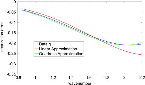
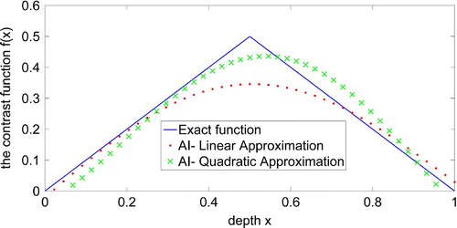
Figure 3. The inverse problem: reconstruction for exact solution (in blue), reconstructed solution for AI linear approximation (in red) and for AI quadratic approximation (in green). The relative errors are ${\mathit{\delta }}_{\mathrm{l}in}=$ 0.1911 and ${\mathit{\delta }}_{\mathrm{q}uad}=$ 0.1079, respectively, with simulated data considered for a wavelength ranging between 350 and 900 nm.

Figure 4. The inverse problem: reconstruction with perturbed data of level 0.15$\%$.

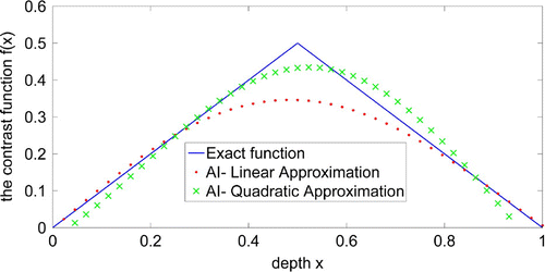
Figure 5. The inverse problem (Adaptive modelling): reconstruction for exact solution (in blue), reconstructed solution for AI linear approximation (in red) and for AI quadratic approximation (in green). The corrections are partially considered. The relative errors are ${\mathit{\delta }}_{\mathrm{l}in}=$ 0.1911 and ${\mathit{\delta }}_{\mathrm{q}uad}=$ 0.0418, respectively.

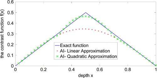
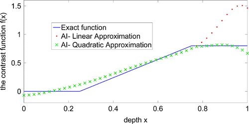
Figure 6. The inverse problem (Adaptive modelling): reconstruction of the Ramp function for exact solution (in blue), reconstructed solution for AI linear approximation (in red) and for AI quadratic approximation (in green). The corrections are partially considered.

shows the outcomes of applying the method of AI to both, linear and quadratic approximations to reconstruct the function $f$. A reconstruction with perturbed data is presented in Figure 4.

6.1. Adaptive modelling

An efficient alternative way to improve the linear approximation is to use a threshold to decide where to apply a higher (quadratic) order of approximation. This leads to what we call adaptive modelling. We take here advantage of the method of the AI which is a local method. Hence, we seek some criterion which evaluates the quality of the linear reconstruction in every part of the function $f$. Such a criterion depends on the validity of the Born approximation. For a fixed frequency, the Born condition depends on the strength of the contrast $f$. By setting another upper bound for the contrast as a threshold, we can locally choose where we need to apply the quadratic approximation. We recall the global validity condition (4.6(4.6) $$\begin{array}{c}\hfill \mathit{\kappa }d\underset{x\in (0,1)}{sup}\left|f(x)\right|<c,\end{array}$$(4.6) )(6.2) $$\begin{array}{c}\hfill \mathit{\beta }\underset{x\in (0,1)}{sup}\left|f(x)\right|<4\mathit{\pi }b,\end{array}$$(6.2)

with $b=0.2$. The aforementioned criterion assumes a stronger condition than (6.2(6.2) $$\begin{array}{c}\hfill \mathit{\beta }\underset{x\in (0,1)}{sup}\left|f(x)\right|<4\mathit{\pi }b,\end{array}$$(6.2) ), namely the computable condition with the linear approximation $f_{\mathrm{l}in}$ of $f$(6.3) $$\begin{array}{c}\hfill \mathit{\beta }\underset{x\in (0,1)}{sup}\left|f_{\mathrm{l}in}(x)\right|<\mathit{\pi }b.\end{array}$$(6.3)

The low contrasts and, respectively, the parts of the function which obey the a-posteriori condition (6.3(6.3) $$\begin{array}{c}\hfill \mathit{\beta }\underset{x\in (0,1)}{sup}\left|f_{\mathrm{l}in}(x)\right|<\mathit{\pi }b.\end{array}$$(6.3) ) are well reconstructed by the linear approximation. For these parts, there is no need to accomplish any approximation of higher order. The quadratic approximation is used then only to improve the reconstruction in these relevant parts, which are beyond the upper bound for the contrast. Comparing Equations (5.8(5.8) $$\begin{array}{c}\hfill f_{\mathit{\gamma }}(x)=〈g,{\mathit{\psi }}_x^{\mathit{\gamma }}〉-\sum _{j=1}^M{\mathit{\psi }}_x^{\mathit{\gamma },j}〈g,C_{j}g〉,\end{array}$$(5.8) ) and (4.10(4.10) $$\begin{array}{cc}\hfill f_{\mathit{\gamma }}(x)& ={〈f,{\mathit{\delta }}_x^{\mathit{\gamma }}〉}_X\hfill \\ \hfill & ={〈f,A^{\ast }{\mathit{\psi }}_x^{\mathit{\gamma }}〉}_X\hfill \\ \hfill & ={〈Af,{\mathit{\psi }}_x^{\mathit{\gamma }}〉}_Y\hfill \\ \hfill & ={〈g,{\mathit{\psi }}_x^{\mathit{\gamma }}〉}_Y=:S_{\mathit{\gamma }}g(x).\hfill \end{array}$$(4.10) ), we see that the corrections $C$ achieved in the quadratic approximation are given by(6.4) $$\begin{array}{c}\hfill C(x)=-\sum _{j=1}^M{\mathit{\psi }}_x^{\mathit{\gamma },j}〈g,C_{j}g〉.\end{array}$$(6.4)

These corrections were computed numerically for each sampling of the generated data. During this numerical computation, the method of Tikhonov–Phillips was used to find the inverse of the ill-conditioned Gram matrix. Thus, we consider the corrections described in Equation (6.4(6.4) $$\begin{array}{c}\hfill C(x)=-\sum _{j=1}^M{\mathit{\psi }}_x^{\mathit{\gamma },j}〈g,C_{j}g〉.\end{array}$$(6.4) ) for the improvement of the reconstruction only in the relevant parts. Figure 5 stands for the comparison between both, the linear and the quadratic approximations, using the idea of the adaptive modelling. See also Figure 6 for the reconstruction of the Ramp function. It is well known that the application of the Born approximation causes artefacts related to a phase shift. Since we are using a method of adjoint field type where the data are in a sense backpropagated from $x=0$, the error is enhanced at $x=1.$ This artefact is more pronounced for the quadratic reconstruction since we apply ${(A_1{A}_1^{\ast })}^{-1}$ when computing the matrices $C_j$ in (5.9(5.9) $$\begin{array}{c}\hfill C_j={(A_1{A}_1^{\ast })}^{-1}{B}_j{(A_1{A}_1^{\ast })}^{-1}.\end{array}$$(5.9) ). This global artefact is clearly reduced when we apply the local method.

7. Conclusion

In this work, we presented an innovative method for the design of ARCs based on solving an inverse nonlinear scattering problem. The main objective in the inverse problem was to determine the space-dependent refractive index of some coating from prescribed reflection coefficients on the surface for multiple frequencies. We applied an iterated Born approximation up to a second order and used the efficient method of AI to deal with both major difficulties in our multi-frequency inverse medium scattering problem, namely the ill-posedness and the nonlinearity. Local corrections which take account of the physical validity of the model provided better results. The tests on simulated data are encouraging to validate the proposed method in industrial applications.

Notes

No potential conflict of interest was reported by the authors.

Department of Mathematics and Statistics, College of Science, King Faisal University, Hofuf, Saudi Arabia.

References

- Chen CJ. Physics of solar energy. Hoboken (NJ): Wiley; 2011.
- Chen D. Anti-reflection (AR) coatings made by sol--gel process. Sol. Energy Mater. Sol. Cells. 2001;68:365–391.
- Bao G, Wang Y. Optimal design of antireflection coatings with different metrics. J. Opt. Soc. Am. A. 2013;30:656–662.
- Dimitriev VI, Chernyavskii AS. Integral characteristic method in the inverse problem of optical coating design. Comput. Math. Model. 2001;12:128–136.
- Nubile P. Analytical design of antireflection coatings for silicon photovoltaic devices. Thin Solid Films. 1999;342:257–261.
- Lesnic D. Determination of the index of refraction of anti-reflection coatings. Math-in-Ind. Case Stud. J. 2010;2:155–173.
- Mahdjoub A, Zighed L. New designs for graded refractive index antireflection coatings. Thin Solid Films. 2005;478:299–304.
- Alakel Abazid M, Lakhal A, Louis AK. Non-destructive testing of anti-reflection coatings for solar cells. In: Proceedings of the European Workshop on Renewable Energy Systems (EWRES). Antalya, Turkey; 2013. pp. 24–28.
- Alakel Abazid M, Lakhal A, Louis AK. A stable numerical algorithm for the design of anti-reflection coatings for solar cells. Int. J. Renew. Technol. in press.
- Janicki V, Sancho-Parramon J, Zorc H. Refractive index profile modelling of dielectric inhomogeneous coatings using effective medium theories. Thin Solid Films. 2008;516:3368–3373.
- Hagin F. Some numerical approaches to solving one-dimensional inverse problems. J. Comput. Phys. 1981;43:16–30.
- Belai OV, Frumin LL, Podivilov EV, Shapiro DA. Inverse scattering for the one- dimensional Helmholtz equation: fast numerical method. Opt. Lett. 2008;33:2101–2103.
- Sacks P. An inverse problem in coupled mode theory. J. Math. Phys. 2004;45:1699–1710.
- Chen Y, Rokhlin V. On the inverse scattering problem for the Helmholtz equation in one dimension. Inverse Prob. 1992;8:365-391.
- Dunn MH, Hariharan SI. Numerical computations on one-dimensional inverse scattering problems. NASA Contractor Rep. 1984;55:157-165.
- Beilina L, Klibanov M. Reconstruction of dielectrics from experimental data via a hybrid globally convergent/adaptive inverse algorithm. Inverse Prob. 2010;26:125009.
- Beilina L, Nguyen TT, Klibanov M and Malmberg JB. Reconstruction of shapes and refractive indices from backscattering experimental data using the adaptivity. Inverse Prob. 2014;30:105007.
- Li J, Xi J, Zou J. An adaptive finite element reconstruction of distributed fluxes. Inverse Prob. 2011;27: 075009 (25pp).
- Born M, Wolf E. Principle of optics. 7th ed. Cambridge (UK): Cambridge University Press; 1999.
- Kak AC, Slaney M. Principles of computerized tomographic imaging. New York (NY): IEEE Press; 1988.
- Natterer F. An error bound for the Born approximation. Inverse Prob. 2004;20:447-452.
- Lakhal A, Louis AK. Locating radiating sources for Maxwell’s equations using the approximate inverse. Inverse Prob. 2008;24: 045020 (18pp).
- Lakhal A. A decoupling-based imaging method for inverse medium scattering for Maxwell’s equations. Inverse Prob. 2010;26:015007.
- Lakhal A. KAIRUAIN-algorithm applied on electromagnetic imaging. Inverse Prob. 2013;29: 095001 (18pp).
- Louis AK. Inverse und schlecht gestellte Probleme [Inverse and ill-posed problems]. Stuttgart: Teubner; 1989.
- Louis AK. A unified approach to regularization methods for linear ill-posed problems. Inverse Prob. 1999;15:489–498.
- Louis AK, Maass P. A mollifier method for linear operator equations of the first kind. Inverse Prob. 1990;6:427–440.
- Louis AK. Approximate inverse for linear and some nonlinear problems. Inverse Prob. 1996;12:175-190.
- Louis AK. Constructing an Approximate Inverse for Linear and Some Nonlinear Problems in Engineering. In: Delaunay D, Jarug Y, Woodbury KA, editors. Inverse Problems in Engineering - Theory and Practice. New York (NY): The American society of Mechanical Engineers; 1998. 367–374.
- Colton D, Kress R. Inverse acoustic and electromagnetic scattering theory. 2nd ed. Berlin: Springer Verlag; 1998.
- Louis AK. Combining image reconstruction and image analysis with an application to two-dimensional tomography. SIAM J. Imag. Sci. 2008;1:188–208.
- Louis AK. Feature reconstruction in inverse problems. Inverse Prob. 2011;27: 065010 (21pp).
- Kohr H. A linear regularization scheme for inverse problems with unbounded linear operators on Banach spaces. Inverse Prob. 2013;29:065015.
- Schuster T, Schöpfer F. Solving linear operator equations in Banach spaces non-iteratively by the method of approximate inverse. Inverse Prob. 2010;26:085006.
- Hahn B, Louis AK. Reconstruction in the three-dimensional parallel scanning geometry with application in synchrotron-based x-ray tomography. Inverse Prob. 2012;28:045013.
- Arridge S, Schotland JC. Topical review: optical tomography: forward and inverse problems. Inverse Prob. 2009;25:123010.
- Jost R. Construction of a potenetial from a phase shift. Phys. Rev. 1952;87.
- Moses HE. Calculating of the scattering potential from reflection coefficients. Phys. Rev. 1956;102:559–567.
- Snieder R. An extension of Backus--Gilbert theory to nonlinear inverse problems. Inverse Prob. 1991;7:409–433.
- Snieder R. The role of nonlinearity in inverse problems. Inverse Prob. 1998;14:387–404.
- Markel VA, O’Sullivan JA, Schotland JC. Inverse problem in optical diffusion tomography. IV. Nonlinear inversion formulas. J. Opt. Soc. Am. A. 2003;20:903–912.
- Moskow S, Schotland JC. Numerical studies of the inverse Born series for diffuse waves. Inverse Prob. 2009;25:095007.