Multi-level backcalculation algorithm for robust determination of pavement layers parameters

Abstract

The backcalculation procedure applied to a mechanical characterization of the road pavement is usually limited to an identification of the elastic modulus of each layer only. The remaining parameters of the model are usually set as known, while performing an inverse analysis. Among assumed parameters are thicknesses of the model layers and frequently considered as constants on a homogeneous section of the road. This is an obvious simplification, because sections in general are inhomogeneous, i.e. the thickness of each layer changes slightly along each road section. Thus the precise and possibly nondestructive estimation of the layers thicknesses is very important and crucial in the inverse procedure. Here, a hybrid form of the optimization algorithm, where the condition of a constant thickness does not need to be fulfilled is described. Further on, the objective function is formed as a discrepancy between reference and computed deflection derivative instead of a deflection curve. In consequence, the values of backcalculated parameters are several per cent more precise compared to a standard procedure. Whenever the thickness of the asphalt layer of the pavement structure cannot be assumed a priori as a constant, the proposed here method appears to be necessary if one does not want to perform costly and destructive in situ drilling tests.

Keywords:

• Inverse analysis
• pavement design
• falling weight deflectomiter
• deflection basin
• deflection curve’s derivative

1. Introduction

The backcalculation analysis is an essential tool of the mechanistic analysis of the road pavements.[1,2] In general, the purpose of an inverse procedure is to determine the causal parameters from the observations of the structure. The measurements in a frame of an in situ pavement testing are often limited to superficial carriageway deflections, while the parameters to be determined are usually stiffness and thickness of each layer. The typical tool applied for the nondestructive evaluation of pavement deflection bowl under the dynamic load is the falling weight deflectometer (FWD). This device is widely used in a civil engineering practice.[3–7] The results of the backcalculation are obtained by minimizing the discrepancy between easily measurable pavement quantities and the corresponding values calculated using analytical or numerical pavement models, e.g. method of equivalent thickness (MET),[8] layered elastic theory (LET),[9] finite element method (FEM),[10] boundary element method (BEM),[11] spectral element method (SEM) [12]).

Each homogeneous layer of the road pavement model can be fully described by the constant thickness and constitutive properties. Due to the relatively simple geometry of carriageway pavements, the analytical or numerical model are most often described in the cylindrical coordinate system. This obviously determines the form of the equilibrium equations of the axisymmetric multilayered half-space. The differential equations describing the mechanics of such models can be found e.g. in [13,14]. In the simple but widely used in the engineering content case of the elastic multilayered model under a static load, totally four independent set of quantities are to be determined, namely: (1) the elastic modulus of each layer, (2) the Poisson’s ratio of each layer, (3) the thickness of each layer, and (4) the parameters defining the quality of the bonding between adjacent layers.

Even in such simplified model, the growing number of layers implies ill-conditioning of the inverse problem from the mathematical perspective. The reason for this issue lies in a well-known compensation effect,[15] which causes that practically any pair of parameters (i.e. layer stiffness and its thickness) can produce similar responses in terms of computed deflections. For this reason, it is common to look for either the values of the elasticity modulus of the model [14,16] or their thickness.[17] By a decoupling of the model parameters into known a priori and sought quantities another important sources of inaccurate identification arise. The most essential ones are due to an imprecise determination of e.g. thickness of the pavement layers [18,19] or a wrong construction or regularization of the objective function.

In the literature, one can find also approaches to identify a full set of model parameters, namely both thicknesses and stiffnesses. The most popular tool used in this content is the artificial neural network (ANN).[20] In this case, limiting the number of simultaneously identifiable parameters has less importance, whereas the crucial is a quality of the database [21] and the performance of the training algorithm. With an appropriately trained ANN structure, it is possible to determine the elastic moduli, thicknesses, and the Poisson’s ratios at the same time.[20] According to the conclusions driven by some authors, e.g. [19], the ANN method is also resistant to the noise resulting from deflection and thickness measurements in-situ. Slightly different approach based on the data mining techniques, proposed in the work [22] provide the value of backcalculation error by several times lower, compared to the values achieved with the use of the linear regression or ANN.

There is also another group of methods, currently under development, in which the thickness of pavement layers is included in a merely indirect way. These methods determine the so-called global parameter,[23] e.g. in the form of a structural number SN (introduced by AASHTO). Some researchers also use deflection basin parameters (DBPs), e.g. surface curvature index (SCI), base damage index (BDI) and base curvature index (BCI).[24] The fact, that these parameters are in strong correlation with the equivalent pavement stiffness , is the basis for simple and empirical backcalculation formulas. However, these methods are developed for a pavement diagnosis purpose and can only serve as a supplement to mechanistic methods.

A disappointing disadvantage of standard procedures in a backcalculation scheme is, the already mentioned, the compensation effect.[15] The result, typical for this phenomenon, can be observed during the careful study of the determined parameters of the pavement model in terms of their values and corresponding discrepancies. Which means that two substantially different converged solutions can result in fairly similar values of the objective function. It becomes then evident that the low values of the mean square error do not, in this case, guarantee reaching the real sought values from an engineering perspective. The use of non-linear elastic constitutive formulation in the pavement multilayer model is considered as a solution to this problem.[15] It is also possible to introduce to the model the so-called stiff layer (bedrock) in order to circumvent the ill-condition formulation of the inverse problem.

The most important ingredients in the inverse analysis are a well-fitted minimization algorithm, which should provide robust and rapid solution. An interesting approach for mechanical identification of the multilayered strata, which is based on a robust system identification method (SIM) is proposed in [25,26]. In both works, the inverse procedure for transverselly isotropic elastic material calibration is utilized. A combination of the dynamic FEM model and nonlocal optimization techniques based on the genetic algorithms is presented in [27], which provides a global minimum of the minimization problem. However, even the most suited algorithms suffer from escalating results of the in-situ deflection measurements. A partial solution to this problem is described in [4], where authors used a probabilistic beckcalculation method combined with a simulation of a measurement test of pavement deflections caused by a dynamic loading. Authors of the work [18] suggest, moreover, that the form of the objective function has a direct influence on the accuracy of backcalculation results. A considerable improvement of the results can be gained by exchanging the root mean square error (RMSE) formula with the area value with correction factor (AVCF) measure, which slightly regularize the problem.

In the commonly used backcalculation procedures of pavement characterization, it is assumed that the thickness of each layer is known. It is also assumed that for the subsequent uniform sections of the pavement they are constant values. In the engineering practice, both the limited accuracy in paving construction technology and the inaccuracies in pavement layers’ thicknesses characterization are the well-known problems, described, e.g. in the work.[28,29] Authors studied the uniform 50-meter long road section and demonstrated that the difference between outliers of the total thickness of the asphalt layers equalled to 3 cm. Therefore, it is very unlikely to conduct an exact synchronization of the real layer thickness (measured or interpolated) with the current location of the in situ deflection curve measurement. Assumption that the thicknesses of the particular model?s layers are constant along the uniform section gives in practice wrong results, which is demonstrated in the conclusions of the work.[30] All those facts imply the need to popularize optimization algorithms in which the thickness of the first layer of the pavement model is determined simultaneously with the values of elastic modulus of each layer.

This paper consists of two separate lines of reasoning and corresponding implementations. The first one is to develop the new computer algorithm capable to fulfil the specified requirements, namely to investigate simultaneously both thicknesses and stiffnesses of the layered pavement structure. Here, the effectiveness of the multilevel minimization algorithm is checked. The first level (outer loop) is responsible for the convergence of the asphalt layer’s thickness while the second level (inner loop) is designed to conduct the traditional investigation of elastic modulus of each layer having thicknesses fixed. In the second thread, the authors discuss the limitations of the backcalculation procedure, based exclusively on the shape of deflection curves. A hypothesis is made that due to the transformation of deflection curves into its derivative curves will improve the accuracy of backcalculation results. The form of the objective function is then expressed with an equation:

2. Methodology

2.1. Pseudo-experimental models

Here, the two fairly similar pavement structures are considered (see Table 1). The pavement’s models have a relatively different set of parameters, which are chosen so that they have possibly identical deflection curves. The assumed values of the Poisson’s ratios are constant, and are equal to = 0.3. The value for all layer’s parameters in the models is shown in Table 1. It is also assumed that there is a full bonding between the model layers.

Table 1. Set of the parameters for two different pavement models analysed in the paper.

	Model A	Model B
[MPa]	7.000	9.368
[MPa]	300	300
[MPa]	100	100
[m]	0.20	0.18
[m]	0.30	0.30

All pseudo-experimental data (used here to mimic the real measurements) were generated by an axisymmetric finite element model with a horizontal and vertical dimension equal to 15 m and 30 m, respectively (detailed studies on the model size are given in [31]). Four nodal axisymmetric finite elements with a full integration scheme are used here along with linear elastic constitutive relationship implemented in each pavement layer. All pseudo-experimental data are subsequently perturbed by random normal distribution of a noise within an interval m. Numerical pseudo-experimental data have, beside the obvious ease in generating, also another very important feature, i.e. the identified parameters from inverse analysis can be straightforwardly compared with those used to generate the model response. The computational tools both for direct and inverse analysis used in this work are the part of the FEMat scientific toolbox.

2.2. Multi-level backcalculation algorithm

Because the backcalculation of the multilayered pavement structure basing on deflections measurements is in general ill-posed, the determination of layer moduli requires having all layers’ thicknesses fixed to the known values. Despite the fact that such logic can be justified, it is still very sensitive to small errors in layer’s thickness estimation. For example, error in estimation generates error in an backcalculation of the elastic modulus . Same error of gives proportional error in characterization. The above observation inspires to design the backcalculation algorithm which will be able to automatically update the model thicknesses to their correct values if initially assumed values are wrong. Here, the investigation is limited to the first layer’s thickness correction only. The general idea of the proposed here procedure is presented in Figure 1.

Figure 1. The scheme used in MLBA procedure.

In order to bring the details of the proposed multi-level backcalculatoin algorithm (MLBA) one needs to discuss also the general framework of inverse analysis and minimization algorithm. Herein, the brief explanation of main features of the inverse procedure followed by a detailed elucidation of implemented minimization algorithms is presented.

Backcalculation analysis with a particular application to constitutive model calibration is a tool widely used by many researchers.[32–39] In general it merges the numerically computed and experimentally determined measurable quantities for a discrepancy minimization. A vector of residua can be constructed in the following way:(1)

This measures the differences between the aforementioned measurable quantities. By adjusting the constitutive parameters (encapsulated in the vector ) embedded in the numerical model, which in turn mimic the experimental setup, an iterative convergence towards the required solution can be achieved. The minimization of the objective function (within the least square frame) takes the form:(2)

and is usually updated through the use of first-order (gradient-based) or zero-order (gradient-less) algorithms. Procedures based on a soft method (e.g. genetic algorithms, simulated annealing, particle swarm algorithms) can be also used for function minimization, especially when the function is non-convex and so has many local minima. However, such algorithms usually require many iterations. Among the many first-order procedures that are based on either the Gauss-Newton or the steepest descent direction in a nonlinear least square methods, the trust region algorithm (TRA) seems the most effective. The TRA uses a simple idea, similar to that in Levenberg-Marquardt (LM) algorithm (see e.g. [40], which performs each new step in a direction combining the Gauss-Newton and steepest descent directions. The LM algorithm computes new directions using the following formula:(3)

where is an internal parameter, is the gradient of the objective function with respect to the parameters (4)

and the Hessian is a second partial derivative of with respect to the parameters :(5)

In the nonlinear least square approach method, the gradient and Hessian matrix can be computed using the Jacobian matrix:(6)

so the gradient and Hessian matrix are defined, respectively:(7)

Such approximation of the Hessian, which can be computed ‘for free’ once the Jacobian is available, represents a distinctive feature of least squares problems. This approximation is valid if the residuals are small, meaning we are close to the solution. Therefore some techniques may be required in order to ensure that the Hessian matrix is semi-positive defined (see e.g. [40]).

One of the main issues of the trust region approach, which to a large extent determines the success and the performance of this algorithm, is in deciding how large the trusted region should be. Allowing it to be too large can cause the algorithm to face the same problem as the classical Newton direction line search, when the model function minimizer is quite distinct from the minimizer of the actual objective function. On the other hand using too small a region means that the algorithm will miss the opportunity to take a step substantial enough to move it much closer to the solution.

Each k-th step in the trust region algorithm is obtained by solving the sub-problem defined by:(8)

where is the trust region radius. By writing the unknown direction as a linear combination of Newton and steepest descent direction, the sub-problem will take the following form:(9)

under the constrains:(10)

The problem now becomes two-dimensional and it is solved for the unknown coefficients and . In order to find both and in Equation (10(10) ) a set of non-linear equations can be solved using, for example, the Newton-Raphson techniques.

As was mentioned in the introductory part of this section the MLBA is a minimization procedure performed on two separate levels. In an internal level the discrepancy between measured and computed quantities is minimized for a fixed value of . In other words, the optimisation algorithm for a given initial value of finds a solution, in terms of three elastic moduli: . The procedure converges when the mean square error reaches its minimum value ( min). This condition, in the classical implementation of inverse analysis, is sufficient to complete the task. According to the authors, however, the analysis should proceed with a different values of in order to find possibly better solution through a multilevel nested analysis. Therefore, in a next step, the optimization algorithm draws another first layer’s thickness and searches for a set of elastic moduli values satisfying the condition . So the converged solution of each internal minimizations brings an objective function value of a single external iteration. On each level, the same minimization algorithm, namely TRA is implemented for discrepancy minimization between computed and measured data (here numerically generated in order to mimic the dynamic FWD measurement test). In order to make an algorithm more sensitive to RMSE, changes in the new concept of deflection slope derivatives will be used herein and briefly explained in the next section.

2.3. Deflection slope derivatives

Most of the methods associated with the backcalculation of pavement’s elastic modulus are related to the direct comparison of deflections curves. Here the new concept is studied which uses the deflection curve’s first derivatives . Such transformation of deflection curve helps to increase the sensitivity of RMSE with respect to the model parameters. Deflections curve is transformed into its first derivative using the forward, central and backward second order of accuracy finite difference in the first point (), all midpoints () and the last one (), respectively, by the following formulas:(11a) (11b) (11c)

The above assumption is an obvious simplification, which introduces a significant error in the derivative estimate of a central point, where its value should be 0 due to axial symmetry of deflection curve. Also derivatives in the vicinity of axis of symmetry are incorrect, however, authors deliberate choice of derivatives (curvatures) computations based on discrete points located on one side of symmetry plane only gives very good indication of models’ differences.

Let’s consider two similar pavement structures with parameters shown in the Table 1. In such a case the RMSE of the two deflections curves has a relatively small value. The difference between both curves is rather small. If one takes the transformed curves, several times increase in the difference in terms of RMSE measurement is observed. The effect of such curve transformation and its influence on RMSE is visualized in Figure 2.

Figure 2. Diagrams for A and B models: (a) the shape of deflection curves, (b) the shape of the curve drawn on the basis of the derivatives of deflection.

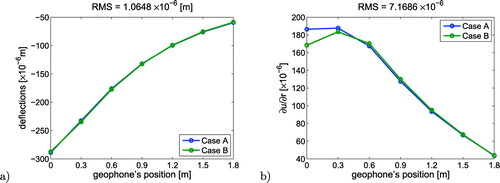
The deflection curves of two pavement models shown in Figure 2a practically overlap though the elastic moduli of first layer which differ more than 33%. Such circumstances reveal that if thickness isn’t correctly measured, the determined elastic modulus can be far different from the real value. In contrary, the deflection line curvature is much more sensitive to model differences and therefore can be more effectively used in thickness estimate correction. Obviously since the difference occurs in the first layer only the most visible curvature deviation are present in the close vicinity of deflection marked in a centre of the load.

3. Numerical results

3.1. Single-level backcalculation approach

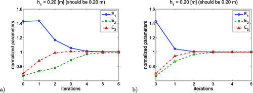
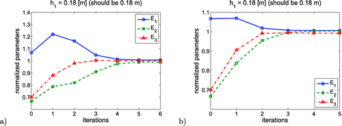
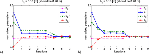
Since the correct values of each elastic modulus are known a-priori, therefore to present the convergence process all computed quantities in each iteration are here divided by their reference values. Thus, if sought parameters converge to one during the minimization process, it means they converge to the exact values. Figures 3 and 4 show the convergence of the minimization procedure based on displacement curves (Figures 3(a) and 4(a), and on derivatives of vertical deflections (Figures 3(b) and 4(b). In all examples, thickness of the first layer was set to the exact value. It meets the standard pavement backcalculation procedure called herein a single-level backcalculation approach (SLBA).

Figure 3. Convergence of the model A parameters (case 11): (a) displacements, (b) derivatives.

Figure 4. Convergence of the model B parameters (case 22): (a) displacements, (b) derivatives.

Table 2 shows detailed converged values of sought parameters in examples given in the Figures 3 and 4. The calculations take into consideration a deflection curve with white noise. The value range of the noise is comprised in .

Table 2. Parameters and backcalculation results in comparison to referential values (A and B Models).

	Case 11			Case 22
	Start	Converged values		Reference	Start	Converged values		Reference
Parameters	values	displ.	deriv.	Model A	values	displ.	deriv.	Model B
[MPa]	10.000	7.026	7.000	7.000	10.000	9.434	9.426	9.368
[MPa]	200	297	300	300	200	297	301	300
[MPa]	70	100	100	100	70	100	99	100
[m]	0.20	–	–	0.20	0.18	–	–	0.18
[m]	0.30	–	–	0.30	0.30	–	–	0.30

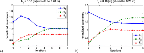
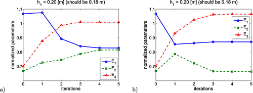
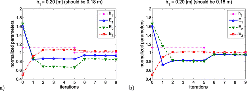
In contrary, Figures 5 and 6 show the convergence process of different models in which the thickness was set to a wrong value. Here, the elastic modulus identified through an inverse analysis has significantly different values than reference ones due to a compensation phenomenon. Setting thickness to lower then reference value automatically generates higher stiffness in order to retain the vertical deflections of the model surface.

Figure 5. Convergence of the model A parameters (case 12): (a) displacements, (b) derivatives.

Figure 6. Convergence of the model B parameters (case 21): (a) displacements, (b) derivatives.

Table 3 shows the detailed converged values of sought parameters in examples given in the Figures 5 and 6. The level of noise of the deflection curves in the pavement model was consistently assumed to be m.

Table 3. Parameters and backcalculation results in comparison to referential values (A and B models).

	Case 12			Case 21
	Start	Converged values		Reference	Start	Converged values		Reference
Parameters	values	displ.	deriv.	Model A	values	displ.	deriv.	Model B
[MPa]	10.000	8.340	8.061	7.000	10.000	7.760	8.164	9.368
[MPa]	200	362	388	300	200	245	199	300
[MPa]	70	100	98	100	70	101	106	100
[m]	0.18	–	–	0.20	0.20	–	–	0.18
[m]	0.30	–	–	0.30	0.30	–	–	0.30

3.2. Multi-level backcalculation approach

Herein, thickness of the first layer model is subjected to a minimization procedure in an external loop, whereas elastic moduli are identified in subsequent internal loops. In each external iteration, a full minimization problem concerning elastic moduli characterization is solved for a fixed value of thickness . Figures 7 and 8 show the convergence of both: (a) thickness and (b) elastic moduli , .

Figure 7. Convergence of the model A parameters (case 12): (a) deflections and (b) derivatives.

The convergence of is observed here within 2–3 iteration (external loop), while elastic moduli are properly determined within 4–5 iterations (internal loop) in each external iteration. In order to speed up the computation the trust region algorithm implemented in an internal minimization loop uses the converged values from the previous external iteration so the convergence curves of elastic moduli depicted in both Figures 7 and 8 form a continuous lines, whereas the curves have characteristic discontinuities. This jumps point out the external iterations.

Figure 8. Convergence of the model B parameters (case 21): (a) deflections, (b) derivatives.

Table 4. Parameters and backcalculation results in comparison to referential values (A and B models).

	Case 12			Case 21
	Start	Converged values		Reference	Start	Converged values		Reference
Parameters	values	displ.	deriv.	Model A	values	displ.	deriv.	Model B
[MPa]	15.000	6.973	6.863	7.000	15.000	8.777	8.941	9.368
[MPa]	500	281	299	300	500	258	290	300
[MPa]	50	100	100	100	50	103	101	100
[m]	0.18	0.2019	0.2015	0.2000	0.20	0.1880	0.1839	0.1800
[m]	0.30	–	–	0.30	0.30	–	–	0.30

Table 4 gather all converged values of sought parameters in these both examples in where the MLBA was applied. Again the noisy data were used ().

3.3. Discussion

When the typical pavement backcalculation procedure is used, the thickness of each layer is assumed as a constant value, therefore the elastic moduli of individual layers are the only unknown parameters to be determined. An inverse analysis performed in such a framework, fits an algorithmic scheme called here the single-level backcalculation approach, which, if tuned with wrong pavement thickness values, converge to the wrong stiffness parameters. The study outlined in this work shows that incorrectly assumed thickness of the first pavement layer (different about two centimetres from its correct value) has a significant influence on the output of the inverse algorithm. The backcalculated values of the elastic moduli are, in this case, substantially under or overestimated, and the RMS value reaches even 30%. This observation applies to both presented here inverse procedure: (a) based on deflection curves and (b) on its derivatives.

The correct values of the sought parameters can be obtained by introducing the proposed here procedure, which uses a multi-level backcalculation algorithm. So both elastic moduli of the pavement layers and the thickness of the first layer are simultaneously investigated. Even though the thickness of the first layer again has been introduced incorrectly (differing by a two centimetres from its correct value), the algorithm precisely converged to the sought parameters (). The subsequent steps in the external loop iteratively updates the thickness and therefore improves the estimates of elastic moduli and in the internal loop. This procedure provides the solution which is considerably more accurate compared to the SLBA. Even better results can be achieved when the derivatives of the deflection curves are used instead of deflection basins itself. Comparing the results achieved basing on the derivatives of the deflection curves, the converged solution is 5% more accurate then corresponding solution computed using deflection curves only.

Analysis and general performance of the proposed multi-level backcalculation algorithm presented here are based on the synthetically generated data. This approach is very often applied to the preliminary testing stage of the new algorithms, mainly because both the sought and model parameters are known a priori and therefore the procedure can be easily checked and confronted. Only knowing precisely each ingredient of the model, i.e. thickness of each layer, its stiffness and Poisson’s ratios, material temperature, interlayer bounds, etc. one can controllably generate pseudo-experimental results (here surface deflections). In the real experimental set-up, it is rather difficult to eliminate all the unknown influences and therefore is rarely used for testing purposes.

4. Conclusions

Knowing the sensitivities of the measurable quantities with respect to the model parameters, one can increase the number of sought parameters to be investigated in an inverse procedure. However, releasing more parameters makes the problem ill-conditioned. The remedy is an iterative procedure updating some parameters in the internal loop while keeping others fixed in the external loop for the subsequent steps. The approach presented here uses this methodology, thus is capable to determine not only the elastic moduli but also the thickness of the asphalt layer.

Based on the selected pseudo-experimental examples of the three-layer pavement models, the novel inverse procedure is proposed here and preliminary tested. The procedure is based on the minimization of the discrepancy between the reference pseudo-experimental (additionally noised) and computed deflection curves. It is noteworthy that an oscillation of measurement’s uncertainties on the level of few micrometers is considered as a noise which can heavily affects the backcalculation results, thus here the noise level is used, which provides stable results. This is an important message showing that while measuring pavement deflections in-situ, one should use a method ensuring the high precision.

In order to identify both the stiffnesses and thicknesses of the pavement model, a new formulation of the multi-level backcalculation algorithm is proposed here.

The proposed algorithm automatically includes the natural changes in the layers’ thickness along the uniform section that results from the construction inaccuracies and defects of the used technology. In the present practice, the in situ destructive test is used to identify the local thickness which is later extrapolated to a uniform section of the road (often hundreds of meters). Therefore the use of the standard backcalculation procedure based on assumed thicknesses, cen results with an error reaching 30%.

In the proposed inverse procedure, the derivatives of the deflection curves are used. This particular construction of the objective function is tested and compared to the traditional implementation based on the deflection curves only. In the case of the standard single-level backcalculation approach, the transformation of the deflection curves does not improve the solution. On the other hand, using the new multi-level backcalculation algorithm produces results that are by a several per cent more precise. For example, providing that the starting value of (asphalt concrete thickness) in the optimization algorithm does not differ from the real one by more than 2 centimetres, the results of the inverse analysis based on the derivatives of deflection curves are more precise than the results achieved by a standard procedure. Taking into account the number of factors affecting the inverse results, the obtained here improvements bring us closer to the more realistic and robust identification of pavement parameters.

Additional information

Funding

This work has been partially supported by the NCBiR research [grant number PBS3/B6/38/2015].

Notes

No potential conflict of interest was reported by the authors.

References

- Lee Y-H, Ker H-W, Lin C-H, et al. Study of backcalculated pavement layer moduli from the LTPP database. Tamkang J. Sci. Eng. 2010;13:145–156.
- Zaghloul S, Helali K, Ahmed R, et al. Implementation of reliability-based backcalculation analysis. J. Transport. Res. Board. 2006;1905:97–106.
- Mun S, Kim YR. Backcalculation of subgrade stiffness under rubblised PCC slabs using multilevel FWD loads. Int. J. Pav. Eng. 2009;10:9–18.
- Hadidi R, Gucunski N. Comparative study of static and dynamic falling weight deflectometer back-calculations using probabilistic approach. J. Transport. Eng. 2010;136:196–204.
- Seo J, Kim Y, Cho J, et al. Estimation of in situ dynamic modulus by using MEPDG dynamic modulus and FWD data at different temperatures. Int. J. Pav. Eng. 2013;14:343–353.
- Tarefder R, Ahmed M. Modeling of the FWD deflection basin to evaluate airport pavements. Int. J. Geomech. 2014;14:205–213.
- Gu X, Wang L, Cheng S, et al. Dynamic response of pavement under FWD using spectral element method. KSCE J. Civ. Eng. 2014;18:1047–1052.
- Ullidtz P. Analytical tools for design of flexible pavements. In: Proceedings of the 9th International conference on asphalt pavements; Copenhagen, Denmark: International Society for Asphalt Pavements; 2002.
- Erlingsson S, Ahmed AW. Fast layered elastic response program for the analysis of flexible pavement structures. Road Mater. Pavement Design. 2013;14:196–210.
- Xu Q, Prozzi JA. A finite-element and Newton-Raphson method for inverse computing multilayer moduli. Finite Elem. Anal. Design. 2014;81:57–68.
- Almeida A, Santos LP. Pavement response excited by road unevennesses using the boundary element method. In: 7th RILEM International conference on cracking in pavements, Vol. 4; 2012. p. 379–388.
- Al-Khoury R, Kasbergen C, Scarpas A, et al. Spectral element technique for efficient parameter identification of layered media: part II: inverse calculation. Int. J. Solids Struct. 2001;38:8753–8772.
- Ayadi AE, Picoux B, Lefeuve-Mesgouez G, et al. An improved dynamic model for the study of a flexible pavement. Adv. Eng. Softw. 2012;44:44–53.
- Tang X, Stoffels SM, Palomino AM. Evaluation of pavement layer moduli using instrumentation measurements. Int. J. Pav. Res. Tech. 2013;6:755–764.
- Ullidtz P, Coetzee NF. Analytical procedures in NDT pavement evaluation, Transportation research record no. 1482 (July 1995). TRB session on structural modelling applications in pavement analysis and design. 1995.
- Hong Z, Wang Y-J, Zhang J-L. A new form of modified iterative method for pavement structure modulus identification. In: Proceeding of the Second international conference on mechanic automation and control engineering (MACE); IEEE. 2010. p. 2769–2772. Issn no. 978-1-4244-7737-1.
- Wang Y, Si H, Su Y, et al. Inverse analysis of pavement thickness based on improved particle swarm optimization. Adv. Mater. Res. 2013;850–851:813–816.
- Sangghaleh A, Pan E, Green R, et al. Backcalculation of pavement layer elastic modulus and thickness with measurement errors. Int. J. Pav. Eng. 2013;15:521–531.
- Ceylan H, Gopalakrishnan K, Bayrak MB, et al. Noise-tolerant inverse analysis models for nondestructive evaluation of transportation infrastructure systems using neural networks. Nondestr. Test. Eval. 2013;28:233–251.
- Saltan M, Uz VE, Aktas B. Artificial neural networks-based backcalculation of the structural properties of a typical flexible pavement. Neural Comput. Appl. 2013;23:1703–1710.
- Gopalakrishnan K, Agrawal A, Ceylan H, et al. Knowledge discovery and data mining in pavement inverse analysis. Transp. 2013;28:1–10.
- Terzi S, Saltan M, Küçüksille E, et al. Backcalculation of pavement layer thickness using data mining. Neural Comput. Appl. 2013;23:1369–1379.
- Moshe L. An alternative forwardcalculation technique as a screening procedure for review and evaluation of backcalculated moduli. Int. J. Roads Airports (IJRA). 2011;1:85–117.
- Talvik O, Aavik A. Use of FWD deflection basin parameters (SCI, BDI, BCI) for pavement condition assessment. Baltic J. Road Bridge Eng. 2009;4:196–202.
- Cai Y, Pan E, Sangghaleh A. Inverse calculation of elastic moduli in cross-anisotropic and layered pavements by system identification method. Inverse Prob. Sci. Eng. 2014;23:718–735.
- Cai Y, Sangghaleh A, Pan E. Effect of anisotropic base/interlayer on the mechanistic responses of layered pavements. Comput. Geotech. 2015;65:250–257.
- Senseney CT, Krahenbuhl RA, Mooney MA. Genetic algorithm to optimize layer parameters in light weight deflectometer backcalculation. Int. J. Geomech. 2013;13:473–476.
- Pożarycki A. Pavement diagnosis accuracy with controlled application of artificial neural network. Baltic J. Road Bridge Eng. 2015;10:355–364.
- Fengier J, Pożarycki A, Garbowski T. Stiff-plate bearing test simulation based on FWD results. Procedia Eng. 2013;57:270–277.
- Zaghloul S, Swan DJ, Hoover T. Enhancing backcalculation procedures through consideration of thickness variability. J. Transport. Res. Board. 2007;0361–1981:80–87.
- Górnaś P, Pożarycki A. The chosen properties of FEM numerical models for backcalculation analysis of road pavement structures. Roads and Bridges - Drogi i Mosty. 3:2014.
- Zirpoli A, Novati G, Maier G, et al. Dilatometric tests combined with computer simulations and parameter identification for in-depth diagnostic analysis of concrete dams. In: Biondini FF, Frangopol D, editors. Life-cycle civil engineering. Proceedings of the 1st International symposium on life-cycle civil engineering, IALCCE 08; London: CRC Press/Balkema, Taylor & Francis Group; 2008, p. 259–264.
- Maier G, Bolzon G, Buljak V, et al. Synergistic combinations of computational methods and experiments for structural diagnosis. In: Kuczma M, Wilmanski K, editors. Advanced structured materials. Proceedings of the 18th international conference on computer methods in mechanics, CMM 2009. Berlin Heidelberg: Springer-Varlag; 2010. p. 453–476.
- Garbowski T, Maier G, Novati G. Diagnosis of concrete dams by flat-jack tests and inverse analyses based on proper orthogonal decomposition. J. Mech. Mater. Struct. 2011;6:181–202.
- Garbowski T, Maier G, Novati G. On calibration of orthotropic elastic-plastic constitutive models for paper foils by biaxial tests and inverse analyses. Struct. Multi. Optim. 2012;46:111–128.
- Gajewski T, Garbowski T. Calibration of concrete parameters based on digital image correlation and inverse analysis. Arch. Civ. Mech. Eng. 2014;14:170–180.
- Gajewski T, Garbowski T. Mixed experimental/numerical methods applied for concreteparameters estimation. In: {\L}odygowski TP, Rakowski J, Litewka P, editors. Recent advances in computationalmechanics. Proceedings of the 20th International conference on computer methods in mechanics, CMM 2013; London: CRC press/Balkema, Taylor & Francis Group; 2014. p. 293–302.
- Knitter-Piatkowska A, Garbowski T. Damage detection through wavelet decomposition and soft computing. In: Moitinho de Almeida JP, D\‘iez P, Par\’es N, editors. Adaptive modeling and simulation. Proceedings of the 6th International conference on adaptive modeling and simulation, ADMOS 2013. International Center for Numerical Methods in Engineering; Barcelona; 2013, p. 389–400.
- Maier G, Buljak V, Garbowski T, et al. Mechanical characterization of materials and diagnosis of structures by inverse analyses: some innovative procedures and applications. Int. J. Comput Methods. 2014. doi:10.1142/S0219876213430020.
- Nocedal J, Wright S. Numerical optimization. 2nd ed. New York (NY): Springer-Verlag; 2006.