Application of artificial bee colony algorithm for inverse modelling of a solar collector

Abstract

This paper deals with the inverse analysis of a double-glazed flat-plate solar collector using the artificial bee colony (ABC) optimization algorithm. In domestic water heating, both low and high heat output from the solar collector is undesirable, so the solar collector is required to supply the hot water at a particular temperature only, which in turn requires a given distribution of heat loss factor. With this criterion, the present analysis is aimed at predicting feasible dimensions and configurations of a solar collector satisfying a prescribed distribution of heat loss factor using ABC algorithm. It is observed that many feasible alternatives of unknowns exist which satisfy a prescribed requirement, and using the ABC algorithm, the size of the solar collector can be minimised by 6–32% with reference to the existing records. The effects of changing ambient conditions are also studied. Furthermore, a comparative study of the ABC algorithm against other heuristic algorithms reveals its suitability and efficacy for the present estimation problem.

Keywords:

• ABC algorithm
• flat-plate solar collector
• inverse analysis
• sensitivity coefficients
• measurement error

1. Introduction

In the present scenario, the area of renewable energy in general and solar energy in particular has gained considerable attention, and is an emerging field of research activity. For harnessing solar energy, flat-plate solar collectors are the most common and simple types which can be effectively used for low-to-medium temperature applications (generally up to 100 °C).[1] Flat-plate solar collectors possess many advantages such as simplicity of construction, high pressure bearing, durability, little maintenance, good heating efficiency and small cost of production.[2] This is the most common type of solar collectors mainly used in building-integrated solar thermal systems[3]; therefore, the same is anticipated to become the key development in the future for building-integrated solar systems.[4,5] Due to these reasons, research on flat-plate solar collectors is receiving considerable surge of interest in the current time.[6–8]

In flat-plate solar collectors, the major percentage of heat loss occurs from the top (i.e. through glass covers), and therefore, for minimising this loss, multiple glazing is provided. In this connection, the evaluation of heat loss factor is an important constituent in the design and simulation of solar collectors.[9] For a given geometry and ambient conditions, the evaluation of heat loss factor directly enables to evaluate the heat lost from the solar collector. In other words, for a given ambient condition, the amount of heat energy available for useful heating can be directly computed once the heat loss factor is known. The heat loss factor is dependent upon the wind, convective and radiative heat transfer coefficients, glass thickness, thermal conductivity of the glass, emissivity of the glazing and absorber plate, etc. Technically, it is quite intuitive that a solar collector should operate at a particular heat loss factor which can offer a desired temperature only. For example, in cold regions, the water needs to be heated which offers a comfortable temperature to the end user and excessive heating (i.e. very low values of heat loss factor) causing discomfort should be avoided. It is quite obvious that ambient conditions generally remain fixed; thus, pertinent dimensions of the solar collector along with surface conditions can be only controlled by the designer.

The design and performance of any engineering equipment depends upon aspects such as thermo-physical parameters and environmental factors. For a specific need, the environmental factors are generally constant in nature and an engineer cannot do much to vary them. Therefore, for achieving a given requirement, the design of equipment is dependent upon thermo-physical parameters of the system. Flexibility in selecting thermo-physical parameters enables the designer to select the appropriate combination of parameters among different existing alternatives. This is because, for a given requirement, at times, various combinations of thermo-physical parameters can yield a similar output.

For estimating and exploring feasible alternatives satisfying a given requirement/objective, an inverse problem is required to be solved.[10] The inverse problems are those in which the objective is to estimate the values of unknown parameters which are essential for satisfying a prescribed condition.[11] In the inverse analysis, multiple combinations of parameters may exist which can fulfil a given requirement.[12] These are mathematically ill-posed, and many examples of such problems are reported in the past.[13] Solution of such problems requires some kind of optimization algorithm.[14]

Optimization methods may be broadly categorised either as classical (gradient-based) and nature-inspired (gradient-free) algorithms. It has been observed that the later fares better in terms of quality of solutions and the independence of assumptions on the search space (particular used for non-convex, discontinuous, non-differentiable types of optimization problems).[15] Nature-inspired optimization algorithms comprise evolutionary algorithms such as genetic algorithms (GA), differential evolution (DE) and simulated annealing (SA). Within the domain of nature-inspired algorithms, a separate area is solely devoted to swarm-based algorithms that deal with the ability of different insects/birds/fishes to solve their real life-related issues. Under this purview, some of the popular optimization methods include the ant colony optimization introduced by Dorigo et al. [16], particle swarm optimization proposed by Kennedy and Eberhart [17], fish swarm algorithm used by Li [18], artificial bee colony (ABC) optimization method presented in 2005 by Karaboga [19], cuckoo search algorithm developed by Yang and Deb [20], and bat and firefly algorithms both initially reported by Yang [21,22]. Among these, ABC is one of the successful and widely used optimization methods of swarm intelligence that mimics the foraging behaviour of real honey bees.[23,24] Honey bees use numerous mechanisms to optimally trace and to explore new food sources in the environment. This feature makes them potential contenders for inventing new search techniques that explore and exploit the search space. ABC possesses many advantages such as high flexibility, ease of implementation, exploring local solutions efficiently, suitability to parallelization, having few control parameters to be tuned along with negligible risk of premature convergence.[25] Moreover, the objective function need not be differentiable and continuous, thereby making ABC one of the robust optimization algorithms. The basic difference between ABC and other conventional evolutionary algorithms such as GA and DE is achieving a good balance between exploration and exploitation, and it has been well established that ABC performs better than their similar counterparts, especially GA.[26]

Based on the above-mentioned background, the objective of this study was to simultaneously optimise five unknown parameters such as the plate–inner glass spacing, inner–outer glass spacing, plate emissivity, tilt angle, plate emittance and the thickness of the glazing in a double-glazed flat-plate solar collector satisfying a given distribution of the heat loss factor. It may be worth to point out that here that this is the first attempt to simultaneously retrieve combination of five parameters satisfying a particular heat loss factor distribution using heuristic algorithm (ABC algorithm for the present work). For a given range of absorber plate temperature, in order to obtain a given value/distribution of the heat loss factor, the above-mentioned five parameters can be adjusted by the designer/operator. Thus, estimating feasible combinations of these parameters enables to predict the collector dimensions and orientation of the collector. In addition to this, the estimation of surface emissivity/emittance provides guidelines about the surface condition which is required to be maintained during the manufacturing process. This is because the surface emittance is dependent upon the surface roughness/ quality.[27,28] The description of the collector and the solution methodology of the present problem are discussed in the subsequent sections.

2. Description of flat-plate solar collector

The schematic diagram of a double-glazed flat-plate solar collector is shown in Figure 1. It consists of an enclosed box with a metal absorber plate (generally made up of anodized aluminium), covered at the top by glass covers. Below the metal plate, there are tubes carrying the working fluid to be heated and insulated at the sides and the bottom. The energy exchange between the glass cover and the metal plate is assumed to occur by convective and radiative heat transfers. Additionally, the heat transfer also occurs between the inner and outer glasses and from the outer glass to the environment by natural convection and radiation. When the collector is exposed to an environment having temperature, T_a, the plate gradually heats up to a temperature, T₁. In this process, inner and outer glass covers also heat up to temperatures, T₂ and T_3, respectively. At steady state, there occurs a heat loss from the collector to the environment due to three major components stated below:

Figure 1. Schematic of double-glazed solar collector.

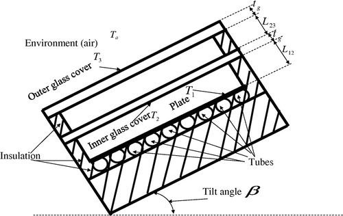
(a) Heat loss from the metal plate to the glass and from the glass to the environment by convection and radiation.

(b) Heat loss within the glass due to conduction.

(c) Heat loss between the two glass covers by convection and radiation (for multiple glazing).

It has been found from many studies that the total heat loss from the collector depends upon many parameters such as the plate–glass spacing (L₁₂), inner–outer glass spacing (L₂₃), the plate emittance $\left({\mathit{\epsilon }}_1\right)$, the tilt angle $\left(\mathit{\beta }\right)$ and the thickness of the glass cover (t_g). Other factors affecting the heat loss are the temperature of the ambient air (T_a), the thermal conductivity of the glazing (k_g) and the wind velocity (v). However, parameters (T_a, k_g and v) remain generally fixed, and therefore, pertinent and controllable design parameters are (L₁₂, L₂₃, ɛ₁, β and t_g). The following section briefly describes the formulation and solution methodology of the present problem.

3. Formulation

A double-glazed flat-plate solar collector has been considered. Under steady state and assuming the sky temperature equal to the ambient, the heat flux, $\ddot{Q}$ between the absorber plate to the inner glass cover, from inner to the outer glass cover and subsequently from the outer glass cover to the ambient air can be, respectively, expressed as indicated below[29]:(1a) $$\ddot{Q}=\left(h_{r,12}+h_{\text{conv}.,12}\right)\left(T_1-T_2\right)$$(1a) (1b) $$\ddot{Q}=\left(h_{r,23}+h_{\text{conv}.,23}\right)\left(T_2-T_3\right)$$(1b) (1c) $$\ddot{Q}=\left\{h_{r,3a}+h_{\text{conv}.,3a}\left(=h_a\right)\right\}\left(T_3-T_a\right)$$(1c)

where h represents the heat transfer coefficient. Subscripts 1, 2, 3 and a are used to represent the absorber plate, inner/first glass cover, second glass cover and ambient condition, respectively. Evaluation of various terms of Equation (1) (such as h_r and h_conv.) has been done using relevant correlations available in [29,30], so these details are not discussed here. For known values of various thermo-physical parameters and ambient conditions, the set of equations may be recursively solved to yield the intermediate glass temperatures ($T_2,T_3$). Then, the total heat loss factor $\left(U_t\right)$ may be calculated using the correlation as mentioned below[30]:(2) $$\begin{array}{c}{U}_t^{-1}={\left[\frac{9.23{\left\{\left(T_1-T_2\right)cos\mathit{\beta }\right\}}^{0.264}}{{\left(T_{M,12}\right)}^{0.46}{L}_{12}^{0.21}}+\frac{4\mathit{\sigma }{T}_{M,12}^3}{\left(\raisebox{1ex}{$1$}\!\left/ \!\raisebox{-1ex}{${\mathit{\epsilon }}_1$}\right.+\raisebox{1ex}{$1$}\!\left/ \!\raisebox{-1ex}{${\mathit{\epsilon }}_g$}\right.-1\right)}\right]}^{-1}+{\left[\frac{9.23{\left\{\left(T_2-T_3\right)cos\mathit{\beta }\right\}}^{0.264}}{{\left(T_{M,23}\right)}^{0.46}{L}_{23}^{0.21}}+\frac{4\mathit{\sigma }{T}_{M,23}^3}{\left(\raisebox{1ex}{$2$}\!\left/ \!\raisebox{-1ex}{${\mathit{\epsilon }}_g$}\right.-1\right)}\right]}^{-1}\\ +{\left[h_a+4\mathit{\sigma }{\mathit{\epsilon }}_g{T}_{M,3a}^3\right]}^{-1}+\frac{2t_g}{k_g}\\ \end{array}$$(2)

where the subscript M denotes the arithmetic mean and represents Stefan–Boltzmann constant. In the above Equation (2(2) $$\begin{array}{c}{U}_t^{-1}={\left[\frac{9.23{\left\{\left(T_1-T_2\right)cos\mathit{\beta }\right\}}^{0.264}}{{\left(T_{M,12}\right)}^{0.46}{L}_{12}^{0.21}}+\frac{4\mathit{\sigma }{T}_{M,12}^3}{\left(\raisebox{1ex}{$1$}\!\left/ \!\raisebox{-1ex}{${\mathit{\epsilon }}_1$}\right.+\raisebox{1ex}{$1$}\!\left/ \!\raisebox{-1ex}{${\mathit{\epsilon }}_g$}\right.-1\right)}\right]}^{-1}+{\left[\frac{9.23{\left\{\left(T_2-T_3\right)cos\mathit{\beta }\right\}}^{0.264}}{{\left(T_{M,23}\right)}^{0.46}{L}_{23}^{0.21}}+\frac{4\mathit{\sigma }{T}_{M,23}^3}{\left(\raisebox{1ex}{$2$}\!\left/ \!\raisebox{-1ex}{${\mathit{\epsilon }}_g$}\right.-1\right)}\right]}^{-1}\\ +{\left[h_a+4\mathit{\sigma }{\mathit{\epsilon }}_g{T}_{M,3a}^3\right]}^{-1}+\frac{2t_g}{k_g}\\ \end{array}$$(2) ), the calculations of glass cover temperatures such as T₂ and T₃ are done in the following manner:(3) $$\begin{array}{c}{T}_3=T_a+h_a^{-0.4}\left(0.0018T_1+0.28{\mathit{\epsilon }}_1-0.37\right)\left(T_1-T_a\right)\\ T_2=T_1-\left(0.7-0.3{\mathit{\epsilon }}_1\right)\left(T_1-T_3\right)\\ \end{array}$$(3)

In any solar collector, parameters such as L₁₂, L₂₃, ɛ₁, β and t_g can be controlled by the designer. Among these five parameters, the evaluation of first four may be quite intuitive. However, the appropriate selection of the last parameter (i.e. the plate emittance) is subjected to the quality and surface conditions of the absorber plate material, because emissivity of a material is invariably dependent upon the surface roughness. An interestingly different situation may be conceived where a given heat transfer characteristic is required to be attained, which is based upon attainment of a pre-defined heat loss factor distribution (say, ${\tilde{U}}_t$). But parameters such as plate–inner glass spacing, L_12; inner–outer glass spacing, L_23; glass thickness, t_g; collector tilt angle, β; and the plate emittance, ɛ_1; are unknown. In order to estimate the feasible values of the five unknown parameters (L₁₂, L₂₃, ɛ₁, β and t_g), a least-squares minimization of the following objective function is required:(4) $$F=\sum _{i=1}^N{\left(U_{t,i}-{\tilde{U}}_{t,i}\right)}^2$$(4)

where N is the number of distinct plate temperatures at which the heat loss factors are computed. In this study, N = 141 equally spaced divisions of plate temperature in the range have been considered. In the present work, the ABC algorithm has been used for minimising Equation (4(4) $$F=\sum _{i=1}^N{\left(U_{t,i}-{\tilde{U}}_{t,i}\right)}^2$$(4) ). The working procedure of ABC algorithm is discussed below.

4. ABC algorithm

Based upon the respective task, in the ABC algorithm, the colony of artificial bees is divided into three groups: (a) employed bees that exploit the food sources (solutions), (b) onlooker bees those watch the dance of employed bees and prefer a potentially high quality food source and (c) scout bees which arbitrarily explore food sources. In ABC, initially (i.e. during initialization phase) a population of employed, onlooker and scout bees (colony) is generated, which may be designated by N_p. The amount of employed bees equals the number of food sources (solutions) because each employed bee is linked with only one food source. In the beginning, all food locations are located by scout bees randomly in the range of each parameter’s lower and upper bound by Equation (5(5) $$x_m=lb+\text{R}\times \left(ub-lb\right)$$(5) ),(5) $$x_m=lb+\text{R}\times \left(ub-lb\right)$$(5)

where $\text{R}\left[0,1\right]$ is a random number. Next, the nectar amount (i.e. fitness/quality of a solution) in food sources is evaluated. Each employed bee collects information related to the vicinity of the food source (V_m) in her memory by conducting a local search by Equation (6(6) $$V_m=x_m+{\mathit{\phi }}_m\times \left(x_m-x_k\right)$$(6) ),(6) $$V_m=x_m+{\mathit{\phi }}_m\times \left(x_m-x_k\right)$$(6)

where φis a random number in [−1, +1] and x_k ≠ x_m is a different food source.

When an employed bee finds a better source (solution) than in her memory, she memorises new source (solution) instead of the old one in a greedy manner. Otherwise, she continues to exploit the source already in her memory. In a real colony, an employed bee unloads the nectar of the source and shares information with the onlookers in the hive about the location and the nectar amount of the source in her memory. Each onlooker bee flies a potentially good food source chosen after watching the dances of employed bees. In ABC, this phenomenon is simulated by assigning a probability value to each source proportional to the fitness of the solution by Equation (7(7) $$P_m=\frac{fi{t}_m\left(x_m\right)}{{\sum }_{m=1}^{N_p/2}fi{t}_m\left(x_m\right)}$$(7) ),[31,32](7) $$P_m=\frac{fi{t}_m\left(x_m\right)}{{\sum }_{m=1}^{N_p/2}fi{t}_m\left(x_m\right)}$$(7)

where, the fitness quantity (nectar amount), $fi{t}_m\left(x_m\right)$ of any food source, x_m, is computed using Equation (8(8) $$fi{t}_m\left(x_m\right)=\left\{\begin{array}{c}\frac{1}{1+F\left(x_m\right)};F\left(x_m\right)>0\\ 1+\left|F\left(x_m\right)\right|;F\left(x_m\right)<0\\ \end{array}\right\}$$(8) ),(8) $$fi{t}_m\left(x_m\right)=\left\{\begin{array}{c}\frac{1}{1+F\left(x_m\right)};F\left(x_m\right)>0\\ 1+\left|F\left(x_m\right)\right|;F\left(x_m\right)<0\\ \end{array}\right\}$$(8)

where F (x_m) is the objective function value. An onlooker bee chooses a food source probabilistically using a selection mechanism such as roulette wheel selection. Once an onlooker bee determines a source, she conducts a local search in the vicinity of the source as in the employed bee phase by Equation (6(6) $$V_m=x_m+{\mathit{\phi }}_m\times \left(x_m-x_k\right)$$(6) ). If a better solution is found, it is replaced by the previous one. When a solution cannot be replaced by a new solution both in employed bee and onlooker bee phases, the solution is continued to be exploited and the nectar of the source exhausts after a number of exploitations. In the ABC algorithm, this is achieved by a control parameter, limit. If a source is exploited as many times as the parameter limit, this source is assumed to be exhausted and the bee of this source becomes a scout. A scout bee finds a random solution by Equation (5(5) $$x_m=lb+\text{R}\times \left(ub-lb\right)$$(5) ).

For flat-plate solar collector problem, in this work, each food source, (m = 1….N_p / 2) consisting 5 variables, is a feasible solution to the problem and the upper and lower bounds for various parameters are mentioned below:(9) $$\left[\begin{array}{c}{L}_{12}-0.015\\ L_{23}-0.015\\ t_g-0.0010\\ {\mathit{\epsilon }}_1-0.100\\ \mathit{\beta }-\mathit{\pi }/18\\ 0.05-L_{12}\\ 0.05-L_{23}\\ 0.006-t_g\\ 0.5-{\mathit{\epsilon }}_1\\ \mathit{\pi }/2-\mathit{\beta }\end{array}\right]\ge 0$$(9)

In Equation (9(9) $$\left[\begin{array}{c}{L}_{12}-0.015\\ L_{23}-0.015\\ t_g-0.0010\\ {\mathit{\epsilon }}_1-0.100\\ \mathit{\beta }-\mathit{\pi }/18\\ 0.05-L_{12}\\ 0.05-L_{23}\\ 0.006-t_g\\ 0.5-{\mathit{\epsilon }}_1\\ \mathit{\pi }/2-\mathit{\beta }\end{array}\right]\ge 0$$(9) ), the minimum limits of the dimensions have been considered to ensure adequate space within the solar collector to allow sufficient convection so that the governing equations hold good. In each cycle of the optimization algorithm, only one scout bee is allowed to occur and the value for limit is 100. The above process constitutes one iteration of the ABC algorithm. In the present work, 500 iterations have been taken as the stopping criterion for the ABC algorithm which has been found to be reasonably sufficient.

5. Results and discussion

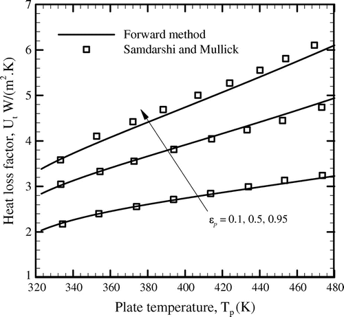
In this section, results on the inverse solution of a double-glazed solar collector problem using the ABC algorithm are presented. In the ABC algorithm, a colony size of N_p = 20 is considered. As mentioned previously, the interest of this work is to simultaneously evaluate five parameters such as the plate–inner glass distance, L_12; inner–outer glass distance, L_23; glass thickness, t_g; the collector tilt angle, β; and the emittance of the absorber plate, ɛ₁; to satisfy a pre-defined distribution of heat loss factor, ${\tilde{U}}_t$. For known values of thermo-physical parameters, the computation of the heat loss factor is obtained by solving Equations 1–3 from a forward approach available in the literature [29,30], and some validations with [30] are presented in Figure 2. For different values of plate emittance, ɛ₁, the results relate to $\mathit{\beta }={45}^{\circ }=0.7854\text{rad}.$, L₁₂ = L₂₃ = 0.025 m, t_g = 3 mm, k_g = 1.02 W/(m·K), h_a = 25 W/(m²·K) and T_a = 303 K from which satisfactory agreement is observed.

Figure 2. Validation of the forward model; T_a = 303 K (30 °C) and h_a = 25 W/(m² K).

Next, considering five parameters (L₁₂, L₂₃, ɛ₁, β and t_g) to be unknowns, an inverse problem has been solved using ABC algorithm. During this analysis, five parameters (L₁₂, L₂₃, ɛ₁, β and t_g) have been considered as unknowns, whereas other pertinent parameters are held the same as the forward analysis. Other pertinent parameters are considered to be known, and they correspond to the validation study. Table 1 presents values of predicted parameters (L₁₂, L₂₃, ɛ₁, β and t_g) computed using the ABC algorithm. Values of these parameters adopted during the forward analysis/validation study against [30] are also mentioned in the table. For each case of measurement error, in this study, five different runs of ABC algorithm have been executed and it is manifested that results differ from one event to another, thereby indicating an ill-posed and non-unique behaviour. Alternatively, many feasible combinations of design and operating parameters are observed to yield a particular distribution of the heat loss factor over the given temperature range. This characteristic enables the designer to discover various viable groups of design parameters meeting a desired objective. However, it can be also revealed from Table 1 that the estimated value of the plate emissivity, ɛ₁, remains almost unique with respect to the one considered in the forward method. This indicates that the plate emittance is a critical parameter which affects the heat loss factor considerably and should be sparingly selected in designing the solar collector. Furthermore, it is revealed that a few combinations of parameters such as runs 3, 5 and 9 of Table 1 yield a total dimension less than that considered in the forward analysis. Therefore, it is evident that through proper adjustment of five design and operating parameters, the size of a solar collector may be reduced by as much as 4–10%.

Table 1. Estimated values of parameters for ambient temperature, T_a = 303 K and wind heat transfer coefficient, h_a = 25 W/(m² K).

Forward method	Without measurement error, e = 0 [L12 m, L23 m, ε1, β rad., tg m]	Total size, m
[L12 = L23 = 0.0250 m, ε1 = 0.1000, β = 0.7850 rad., tg = 0.0030 m]	Run 1: [0.0402,0.0256,0.1000,0.1745,0.0036]	0.0730
	Run 2: [0.0377,0.0307,0.1000,0.2436,0.0036]	0.0756
	Run 3: [0.0205,0.0213,0.1129,0.9308,0.0060]	0.0538
	Run 4:[ 0.0358,0.0493,0.1004,0.1746,0.0031]	0.0913
	Run 5: [0.0300, 0.0170,0.1000,0.6968,0.0036]	0.0542
Total size = 0.0560 m	With measurement error, e ≠ 0
	Run 6: [0.0274,0.0500,0.1000,0.3496,0.0060]	0.0894
	Run 7: [0.0182,0.0500,0.1000,0.8478,0.0038]	0.0758
	Run 8: [0.0232,0.0290,0.1000,0.6864, 0.0056]	0.0634
	Run 9: [0.0247,0.0195,0.1000,0.8223,0.0031]	0.0504
	Run 10: [0.0288,0.0500,0.1000,0.5134,0.0033]	0.0854

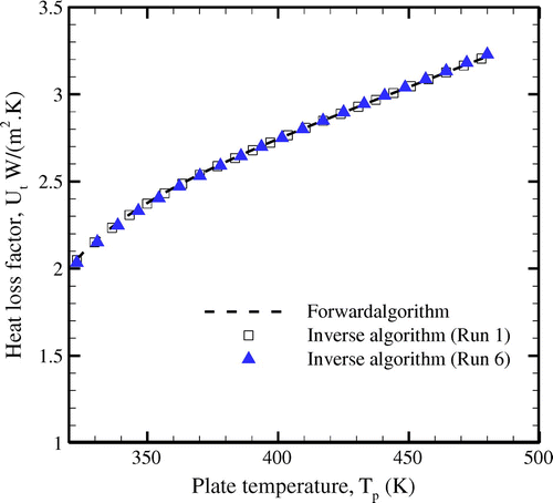
The estimated values of five parameters are meaningful, if each one of them yields the required heat transfer requirement as revealed by the heat loss factor. So, in order to examine the variation between the actual heat loss factor distribution, ${\tilde{U}}_t$ and the one pertaining to the inversely estimated values of unknown parameters (L₁₂, L₂₃, ɛ₁, β and t_g), an evaluation has been carried out in Figure 3. The heat loss factor that has been computed from the forward method by inputting the inversely-estimated values of unknown parameters (L₁₂, L₂₃, ɛ₁, β and t_g) is known as the reconstructed distribution. For better visualisation, results have been shown only for runs 1 and 6 of Table 1. For different levels of plate temperatures, T_p, it can be revealed from Figure 3 that a very good agreement occurs between actual and the reconstructed distributions.

Figure 3. Comparison of exact and reconstructed heat loss factor distributions; T_a = 303 K (30 °C) and h_a = 25 W/(m² K).

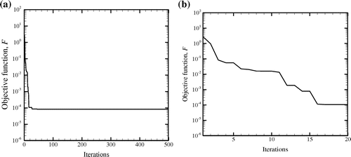
In order to demonstrate the change of the objective function, F, in course of the optimization process of ABC algorithm, a comparison is depicted in Figure 4. The result pertains to Run 1 of Table 1. For this study, 500 iterations of the ABC algorithm have been used as the termination criteria, which are observed to be sufficient. It can be noticed from Figure 4(a) that the objective function, F, minimises from a higher value to approximately O (10⁻⁵) in 500 iterations. Furthermore, it is also seen that the objective function attains O (10⁻⁴) in just 20 iterations of the ABC algorithm (Figure 4(b)). So between 20 and 500 iterations, there is only marginal change in the objective function, F. This reveals that the position cannot be significantly improved beyond 20 iterations, which is referred to as the limit For abandonment (LFA) implying that food source is abandoned and the scout is unable to determine a fresh food source location randomly.[15]

Figure 4. Variation of the objective function with iterations of ABC algorithm (noise-free case); (a) history of 500 iterations, (b) history of first 20 iterations; T_a = 303 K (30 °C) and h_a = 25 W/(m² K).

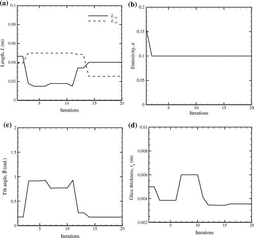
The iteration-wise variations of five parameters (L₁₂, L₂₃,ɛ₁, β and t_g) which have been inversely estimated using ABC algorithm are depicted in Figure 5. These results relate to Run 1 of Table 1 corresponding to which the applicable objective function variation, F, is demonstrated previously in Figure 4. Since the objective function variation was significant for the first 20 iterations only, parametric variations have been also presented for 20 iterations in Figure 5. It has been perceived from these figures that all five parameters (L₁₂, L₂₃, ɛ₁, β and t_g) are subjected to a continuous change during the range of first 20 iterations, but they seldom change beyond this due to the attainment of the LFA, as discussed earlier. Except the plate emittance whose value does not change after 1st iteration, all other parameters undergo change at some point of time during first 20 iterations.

Figure 5. Variation of estimated parameters with iterations of ABC algorithm (noise-free case); T_a = 303 K (30 °C) and h_a = 25 W/(m² K).

After successfully demonstrating the suitability of ABC algorithm in estimating pertinent design parameters satisfying a given distribution of heat loss factor, the effect of random noise has been considered next. In actual practice, the measurement of absorber plate temperature, T₁, is vulnerable to measurement error, which in turn includes error in the analytical prediction of heat loss factor distribution, U_t. 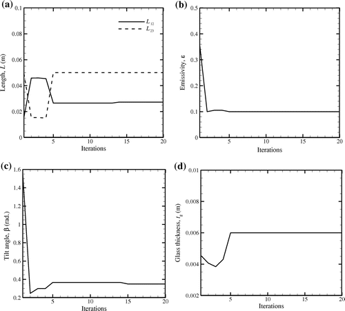So random errors $\left(-11\%<e<+11\%\right)$ following an additive white Gaussian distribution have been incorporated to the exact distribution of heat loss factor, ${\tilde{U}}_t$ and the resulting noise-induced distribution is shown in Figure 6. Figures 7 and 8 indicate variation of the objective function, F, along with five parameters (L₁₂, L₂₃,ɛ₁, β and t_g) during the optimization process of the ABC algorithm considering a noise-induced distribution of the heat loss factor. It can be revealed from Figure 7 that only after five iterations, the function value minimises to O(10⁻¹) and even after 500 iterations of ABC, its value does not change appreciably.

Figure 6. Comparison of exact and reconstructed heat loss factor distributions; $\mathit{\beta }={45}^{\circ }=0.7854\text{rad}.$, L₁₂ = L₂₃ = 0.025 m, t_g = 3 mm, k_g = 1.02 W/(m K), T_a = 303 K (30 °C) and h_a = 25 W/(m² K).

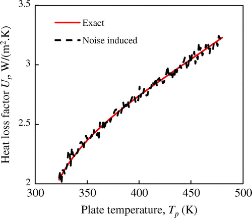
Figure 7. Variation of the objective function with iterations of ABC algorithm (noise-induced case) for Run 6 of Table 1; (a) history of 500 iterations, (b) history of first 20 iterations; T_a = 303 K (30 °C) and h_a = 25 W/(m² K).

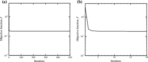
Figure 8. Variation of estimated parameters with iterations of ABC algorithm (noise-induced case) for Run 6 of Table 1; T_a = 303 K (30 °C) and h_a = 25 W/(m² K).

It is quite perceptive from the above discussion that the dependency of the heat loss factor, U_t, on five estimated parameters (L₁₂, L₂₃,ɛ₁, β and t_g) shall be of different magnitudes. The study of sensitivity coefficient is an important constituent in inverse analyses. The sensitivity coefficient for any parameter (say the tilt angle, β) on the heat loss factor can be expressed as below:(10) $$S_{\mathit{\beta }}={\left.\frac{\mathit{\partial }{U}_t}{\mathit{\partial }\mathit{\beta }}\right|}_{\left(L_{12},L_{23},{\mathit{\epsilon }}_1,t_g=\text{constants}\right)}$$(10)

In the present study, for computing the sensitivity coefficient, a small change (1%) has been made to the relevant parameter for which the sensitivity coefficient is required to be obtained. 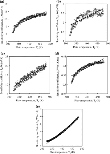Then, the difference between the old and new heat loss factors is found, which after division by the change in the particular parameter, the final sensitivity coefficient is obtained using Equation (10(10) $$S_{\mathit{\beta }}={\left.\frac{\mathit{\partial }{U}_t}{\mathit{\partial }\mathit{\beta }}\right|}_{\left(L_{12},L_{23},{\mathit{\epsilon }}_1,t_g=\text{constants}\right)}$$(10) ). Further details about sensitivity coefficients can be found elsewhere,[33,34] so these details are not repeated here. Figure 9 presents the sensitivity coefficients for different parameters (L₁₂, L₂₃, ɛ₁, β and t_g) considered and estimated in the present work. The respective trend lines have been also indicated. It may be easily noted that the sensitivity coefficient of the absorber plate emissivity, S_ɛ1, is considerably higher than that for other four parameters. This is followed by the plate–inner glass spacing, glass thickness, inner glass–outer glass spacing and the collector tilt angle. Based on the involvement of the absorber plate in first two highest sensitivity coefficients (i.e. plate emissivity and plate–inner glass spacing), this study infers that the absorber plate is a critical component in controlling the behaviour of the solar collector. This finding is also in accordance with results presented in Table 1 in which nearly unique estimation of the plate emissivity was observed, whereas a wide range of scopes were available for the tilt angle. The second observation from Figure 9 is that the trend lines of sensitivity coefficient always increase with the absorber plate temperature which is due to the reason of enhanced heat loss at higher temperatures, thereby requiring an accurate prescription of temperatures at such positions.[33] The conclusion of the present work is discussed below.

Figure 9. Comparison of sensitivity coefficients of different estimated parameters; $\mathit{\beta }={45}^{\circ }=0.7854\text{rad}$, L₁₂ = L₂₃ = 0.025 m, t_g = 3 mm, k_g = 1.02 W/(m K), T_a = 303 K (30 °C) and h_a = 25 W/(m² K).

In order to assess the suitability of ABC algorithm for the present problem, a study has been carried out in Table 2. The study has been done for the case involving no measurement error, i.e. e = 0. The present work involves difficulty mainly due to the presence of non-linearity of radiative heat transfer mode. Apart from ABC algorithm, the estimated parameters have been obtained using the GA,[35] the SA algorithm [36] and the DE algorithm.[37] For this comparison, the population size has been considered to be the same as the colony size (i.e. N_p = 20) of the present ABC algorithm. In the GA, the crossover probability of 0.80 and the mutation probability of 0.03 have been considered,[35] whereas in the DE, the crossover probability of 0.90 and the scaling factor of 0.80 were taken.[37] The re-annealing schedule to lower the temperature level in the SA has been considered to be 0.95 of the previous level.[36] For this comparison, the termination condition for all four optimization has been fixed as 500 iterations, and thus, results have been obtained after 500 iterations of each algorithm. It may be observed from Table 2 that many feasible combinations are obtained from different algorithms, but ABC-based algorithm could yield a reduced collector size as compared to the one considered for the forward solution. For each optimization algorithm compared in Table 2, the corresponding iterative variation of the objective function, F, has been presented in Figure 10. It is revealed from the figure that ABC algorithm performs better in minimising the objective function to a lower than that done by other algorithms such as GA, DE and SA. In order to further investigate the performance of the four methods (GA, DE, SA and ABC), ten distinct runs have been considered in Table 3. It is observed from the table that on five of ten runs, the ABC yields relatively better performance than other algorithms. The DE performs better on three runs, whereas the GA and the SA outperform others on only one occasion each. Furthermore, for the present work, the averaged objective function value, F_avg,_. corresponding to the ABC algorithm has been found to be less as compared to other three algorithms, as revealed from Table 3.

Table 2. Comparison of estimated parameters and objective functions obtained with different optimization methods after 500 iterations.

Forward method	Genetic algorithm	DE algorithm	SA algorithm	ABC algorithm
[L12 = L23 = 0.0250 m, ε1 = 0.1000,  = 0.7850 rad., tg = 0.0030 m]	[L12 = 0.0330 m, L23 = 0.0229 m, ε1 = 0.1007, β = 0.6000 rad., tg = 0.0027 m]	[L12 = 0.0379 m, L23 = 0.0309 m, ε1 = 0.1001, β = 0.2546 rad., tg = 0.0036 m]	[L12 = 0.0249 m, L23 = 0.0269 m, ε1 = 0.1000, β = 0.8250 rad., tg  = 0.0021 m]	[L12 = 0.0209 m, L23 = 0.0200 m, ε1 = 0.1096, β = 0.9061 rad., tg  = 0.0059 m]
	F = 1.800 × 10^−3	F = 1.643 × 10^−3	F = 5.500 × 10^−3	F = 2.939 × 10^−4
Total size 0.0560 m	Total size 0.0613 m	Total size 0.0760 m	Total size 0.0560 m	Total size 0.0527 m

Figure 10. Comparison of objective functions for different optimization algorithms (a) history of 20 iterations, (b) history of 500 iterations; T_a = 303 K (30 °C) and h_a = 25 W/(m² K).

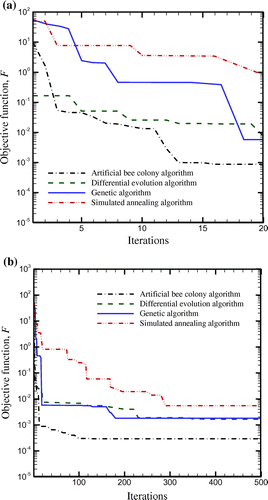
Table 3. Comparison of different optimization methods for 10 additional runs (500 iterations in each case).

Run No.	Genetic algorithm: [L12, L23, ε1, β, tg]; F	DE algorithm: [L12, L23, ε1, β, tg]; F	SA algorithm: [L12, L23, ε1, β, tg]; F	ABC algorithm: [L12, L23, ε1, β, tg]; F
1	[0.0371 m, 0.0355 m, 0.1133, 0.4787 rad., 0.0044 m]; F = 6.300 × 10^−3,(size = 0.0814 m)	[0.0388 m, 0.0299 m, 0.1029, 0.1929 rad., 0.0042 m]; F = 8.805 × 10^−5,(size = 0.0771 m)	[0.0266 m, 0.0204 m, 0.1028, 0.7667 rad., 0.0041 m]; F = 2.938 × 10^−4, (size = 0.0552 m)	[0.0393 m, 0.0267 m, 0.1022, 0.2162 rad., 0.0041 m]; F = 1.569 × 10^−4(size = 0.0742 m)
2	[0.0309 m, 0.0420 m, 0.1067, 0.5626 rad., 0.0039 m]; F = 7.667 × 10^−4, (size = 0.0807 m)	[0.0363 m, 0.0363 m, 0.1000, 0.3155 rad.,0.0030 m]; F = 1.065 × 10^−5, (size = 0.0786 m)	[0.0339 m, 0.0286 m, 0.1008, 0.4956 rad., 0.0031 m]; F = 9.022 × 10^−4, (size = 0.0687 m)	[0.0369 m, 0.0266 m, 0.1048, 0.3764 rad., 0.0047 m];F = 3.210 × 10^−5, (size = 0.0729 m)
3	[0.0234 m, 0.0206 m, 0.1083, 0.8461 rad., 0.0050 m]; F = 6.300 × 10^−3, (size = 0.0540 m)	[0.0269 m, 0.0390 m, 0.1000, 0.7081 rad., 0.0020 m]; F = 5.933 × 10^−4, (size = 0.0699 m)	[0.0434 m, 0.0237 m, 0.1054, 0.2905 rad., 0.0030 m]; F = 8.401 × 10^−3, (size = 0.0731 m)	[0.0346 m, 0.0388 m, 0.1034, 0.3743 rad., 0.0040 m]; F = 3.796 × 10^−4, (size = 0.0814 m)
4	[0.0209 m, 0.0276 m, 0.1027, 0.8751 rad., 0.0039 m]; F = 5.304 × 10^−4, (size = 0.0563 m)	[0.0368 m, 0.0295 m, 0.1039, 0.3671 rad., 0.0040 m]; F = 8.942 × 10^−4, (size = 0.0743 m)	[0.0359 m, 0.0189 m, 0.1078, 0.5503 rad., 0.0050 m]; F = 8.823 × 10^−4, (size = 0.0648 m)	[0.0420 m, 0.0192 m, 0.1069, 0.2594 rad., 0.0053 m]; F = 6.251 × 10^−4, (size = 0.0718 m)
5	[0.0317 m, 0.0455 m, 0.1090, 0.5126 rad., 0.0046 m]; F = 9.667 × 10^−4, (size = 0.0864 m)	[0.0394 m, 0.0309 m, 0.1049, 0.2636 rad., 0.0040 m]; F = 4.129 × 10^−4, (size = 0.0783 m)	[0.0315 m, 0.0401 m, 0.1017, 0.5847 rad., 0.0021 m]; F = 1.276 × 10^−3, (size = 0.0758 m)	[0.0334 m, 0.0333 m, 0.1000, 0.4712 rad., 0.0030 m]; F = 3.165 × 10^−5, (size = 0.0727 m)
6	[0.0245 m, 0.0215 m, 0.1017, 0.7975 rad., 0.0041 m]; F= 1.967 × 10^−4, (size = 0.0542 m)	[0.0338 m, 0.0308 m, 0.1044, 0.4756 rad., 0.0043 m]; F = 6.147 × 10^−5, (size = 0.0732 m)	[0.0375 m, 0.0354 m, 0.1133, 0.4787 rad., 0.0043 m]; F=6.400 × 10^−3, (size = 0.0815 m)	[0.0366 m, 0.0250 m, 0.1027, 0.3922 rad., 0.0043 m]; F = 2.317 × 10^−5, (size = 0.0702 m)
7	[0.0334 m, 0.0204 m, 0.1038, 0.5701 rad., 0.0045 m]; F = 5.234 × 10^−5, (size = 0.0628 m)	[0.0349 m, 0.0260 m, 0.1028, 0.4636 rad., 0.0040 m]; F = 5.831 × 10^−4, (size = 0.0689 m)	[0.0246 m, 0.0280 m, 0.1104, 0.8144 rad., 0.0046 m]; F = 3.900 × 10^−3, (size = 0.0618 m)	[0.0347 m, 0.0346 m, 0.1000, 0.4078 rad., 0.0030 m]; F = 8.997 × 10^−6, (size = 0.0753 m)
8	[0.0393 m, 0.0245 m, 0.1008, 0.2032 rad., 0.0043 m]; F = 6.559 × 10^−4, (size = 0.0724 m)	[0.0150 m, 0.0150 m, 0.1027, 1.0480 rad., 0.0050 m]; F = 3.146 × 10^−3, (size = 0.040 m)	[0.0359 m, 0.0297 m, 0.1014, 0.3908 rad., 0.0036 m]; F = 7.762 × 10^−6, (size = 0.0728 m)	[0.0356 m, 0.0196 m, 0.1049, 0.5064 rad., 0.0049 m]; F= 4.107 × 10^−5, (size = 0.0650 m)
9	[0.0293 m, 0.0440 m, 0.1000, 0.5604 rad., 0.0028 m]; F = 1.684 × 10^−4, (size = 0.0789 m)	[0.0348 m, 0.0347 m, 0.1000, 0.4004 rad., 0.0030 m]; F = 4.951 × 10^−5, (size = 0.0755 m)	[0.0403 m, 0.0216 m, 0.1007, 0.3191 rad., 0.0033 m]; F = 8.907 × 10^−4, (size = 0.0685 m)	[0.0356 m, 0.0352 m, 0.1057, 0.3457 rad., 0.0048 m]; F = 4.148 × 10^−4, (size = 0.0804 m)
10	[0.0319 m, 0.0289 m,0.1138, 0.6112 rad., 0.0059 m]; F = 1.551 × 10^−3, (size = 0.0726 m)	[0.0312 m, 0.0208 m, 0.1019, 0.6227 rad., 0.0041 m]; F = 8.322 × 10^−5, (size = 0.0602 m)	[0.0158 m, 0.0409 m, 0.1056, 0.9904 rad., 0.0040 m]; F = 3.260× 10^−3, (size = 0.0647 m)	[0.0331 m, 0.0331 m,0.1000, 0.4852 rad., 0.0030 m]; F = 1.021 × 10^−5, (size = 0.0722 m)
	Average function, Favg. = 1.748 × 10^−3	Average function, Favg. = 5.922 × 10^−4	Average function, Favg. = 2.621 × 10^−3	Average function, Favg. = 1.723 × 10^−4

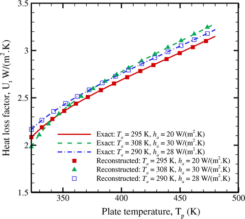
To assess the effect of variation in ambient conditions due to change in the ambient temperature, T_a, along with variable wind speed that yields different values of the wind heat transfer coefficient, h_a, a study has been presented in Table 4. The study has been made assuming the heat loss factor to be free of measurement error. The results have been shown after 500 iterations of the ABC algorithm. Various sets of ambient temperatures along with wind heat transfer coefficients are also indicated in the same table. It is observed that the results are in line with those obtained earlier in Table 1. However, here the opportunity of reducing the solar collector size is observed to be approximately 32%, as observed in Run 1 of Table 4. Furthermore, from the analysis of objective functions, there is no significant variation in the value of objective function beyond 20 iterations, as observed from Figure 11. Similar to previous observation made in Figure 7, in this case too, the objective function, F, attains O(10⁻⁴) in 20 iterations. For different sets of ambient conditions considered in Table 3, the iterative variations of five estimated parameters (L₁₂, L₂₃, ɛ₁, β and t_g) are shown in Figures 12–14. Figure 15 presents the comparison of the exact and the reconstructed distributions of heat loss factor under changing environmental conditions. For the case involving no measurement error, the trends have been shown for the ABC-estimated results presented in Table 4. It is found that the reconstructed heat loss factor distributions obtained from the inversely estimated parameters yield a very good agreement with the exact ones, under diverse ambient conditions.

Table 4. Estimated values of parameters for variable ambient conditions.

Forward method	[L12 m, L23 m, ε1, β rad., tg m]	Total size, m
[L12 = L23 = 0.0250 m, ε1 = 0.1000, β = 0.7850 rad., tg = 0.0030 m] Total size = 0.0560 m	Ta = 295 K (22 °C), ha = 20 W/(m^2.K) Run 1: [0.0150,0.0150,0.1000,1.0617,0.0039]	0.0378
	Ta = 308 K (35 °C), ha = 30 W/(m^2.K) Run 2: [0.0333,0.0498,0.1000,0.4569,0.0017]	0.0865
	Ta = 290 K (17 °C), ha = 28 W/(m^2.K) Run 3: [0.0272,0.0171,0.1000,0.7657,0.0037]	0.0517

Figure 11. Comparison of objective functions for solar collector operating under varying ambient conditions (a) history of 200 iterations, (b) history of first 20 iterations.

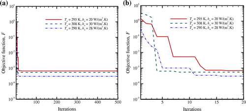
Figure 12. Variation of estimated parameters for ambient temperature, T_a = 295 K (22 °C) and wind heat transfer coefficient, h_a = 20 W/(m² K).

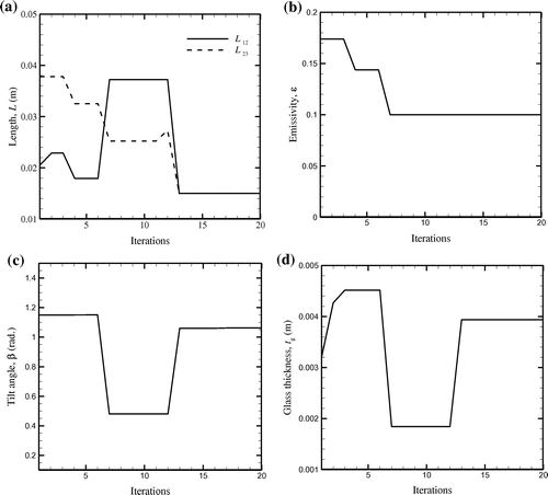
Figure 13. Variation of estimated parameters for ambient temperature, T_a = 308 K (35 °C) and wind heat transfer coefficient, h_a = 30 W/(m² K).

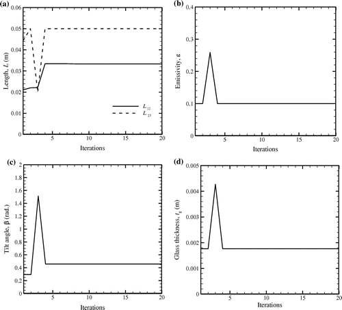
Figure 14. Variation of estimated parameters for ambient temperature, T_a = 290 K (17 °C) and wind heat transfer coefficient, h_a = 28 W/(m² K).

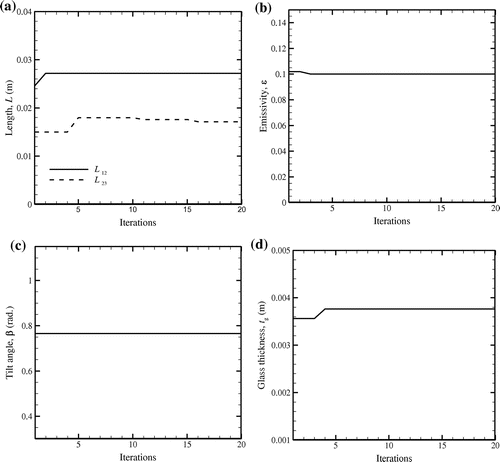
Figure 15. Comparison of exact and reconstructed heat loss factor distributions under different environmental conditions.

6. Conclusion

An inverse analysis is carried out to estimate important and adjustable parameters of a double-glazed flat-plate solar collector using the ABC algorithm. A flat-plate solar collector being a preferable choice for building-integrated solar systems and due to undesirability of both low and high heat output particularly in domestic water heating, it is required to operate at a given heat loss factor. In this study, feasible dimensions and configurations of a solar collector satisfying a prescribed heat loss factor distribution have been estimated using the ABC algorithm and there exists an opportunity to minimise the size of the solar collector. The effects of ambient condition variations resulting in temperature along with wind speed or wind heat transfer coefficient changes have been also considered. The study also reveals that the absorber plate is a critical constituent whose emissivity significantly controls the attainment of the heat loss factor. Additionally, a comparison of the ABC algorithm with other heuristic optimization methods demonstrates the suitability of the ABC for the present problem involving five unknown parameters. However, for minimising the collector size and acquiring a given heat loss factor, a wide range of alternatives is available for adjusting the collector tilt angle.

Nomenclature
e	=	measurement error
F	=	objective function
h	=	heat transfer coefficient $\left(\text{W}·{\text{m}}^{-2}·{\text{K}}^{-1}\right)$
k	=	thermal conductivity $\left(\text{W}·{\text{m}}^{-1}·{\text{K}}^{-1}\right)$
L	=	length (m)
(lb, ub)	=	lower and upper bounds
N	=	number of discrete temperatures
Np	=	colony size
P	=	probability in ABC algorithm
$\ddot{\mathit{Q}}$	=	heat flux$\left(\text{W}·{\text{m}}^{-2}\right)$
R	=	random number in ABC algorithm
S	=	sensitivity coefficient
T	=	temperature (K)
t	=	thickness of the glass cover (m)
U	=	heat loss factor $\left(\text{W}·{\text{m}}^{-2}·{\text{K}}^{-1}\right)$
v	=	wind velocity (m/s)
V	=	location of new food source in ABC
x	=	location of old food source in ABC

Greek symbols

β	=	collector tilt angle (radians)
ɛ	=	emissivity of the fin material
σ	=	Stefan-Boltzmann constant $\left(\text{W}·{\text{m}}^{-2}·{\text{K}}^{-4}\right)$

Subscripts and superscripts

1	=	absorber plate
2	=	inner glass cover
3	=	outer glass cover
a	=	ambient condition
avg.	=	average value
conv.	=	convection
g	=	glass cover
M	=	arithmetic mean
m	=	index for a given food source
r	=	radiation
~	=	exact value

Disclosure statement

No potential conflict of interest was reported by the authors.

References

- Sekhar YR, Sharma KV, Rao MB. Evaluation of heat loss coefficients in solar flat plate collectors. ARPN J. Eng. Appl. Sci. 2009;4:15–19.
- Jiandong Z, Hanzhong T, Susu C. Numerical simulation for structural parameters of flat-plate solar collector. Sol. Energy. 2015;117:192–202.10.1016/j.solener.2015.04.027
- Visa I, Duta A, Comsit M, et al. Design and experimental optimisation of a novel flat plate solar thermal collector with trapezoidal shape for facades integration. Appl. Therm. Eng. 2015;90:432–443.10.1016/j.applthermaleng.2015.06.026
- Yang Y, Wang Q, Xiu D, et al. A building integrated solar collector: all-ceramic solar collector. Energy Build. 2013;62:15–17.10.1016/j.enbuild.2013.03.002
- Zhai XQ, Wang RZ, Dai YJ, et al. Solar integrated energy system for a green building. Energy Build. 2007;39:985–993.10.1016/j.enbuild.2006.11.010
- Neagoe M, Visa I, Burduhos BG, et al. Thermal load based adaptive tracking for flat plate solar collectors. Energy Procedia. 2014;48:1401–1411.10.1016/j.egypro.2014.02.158
- Chen G, Doroshenko A, Koltun P, et al. Comparative field experimental investigations of different flat plate solar collectors. Sol. Energy. 2015;115:577–588.10.1016/j.solener.2015.03.021
- Deng J, Xu Y, Yang X. A dynamic thermal performance model for flat-plate solar collectors based on the thermal inertia correction of the steady-state test method. Renew. Eng. 2015;76:679–686. 10.1016/j.renene.2014.12.005
- Usmani AY, Akhtar N. Existing correlations of top heat loss factor of flat plate solar collectors and impact on useful energy. Int. J. Emergency Technol. Adv. Eng. 2013;3:607–612.
- Das R. Inverse study of double-glazed solar collector using hybrid evolutionary algorithm. IEEE Seventh International Conference on Contemporary Computing (IC3); Noida, India. 2014. p. 571–576.
- Noh M-H, Lee S-Y. A bivariate Gaussian function approach for inverse cracks identification of forced-vibrating bridge decks. Inverse Probl. Sci. Eng. 2013;21:1047–1073.10.1080/17415977.2012.727086
- Das R, Ooi KT. Predicting multiple combination of parameters for designing a porous fin subjected to a given temperature requirement. Energy Convers. Manage. 2013;66:211–219. 10.1016/j.enconman.2012.10.019
- Choi J-H, Jung Y-J, Jung H-K, et al. A new multimodal cortical source imaging algorithm for integrating simultaneously recorded EEG and MEG. Inverse Probl. Sci. Eng. 2013;21:1074–1089.10.1080/17415977.2012.731596
- El Zahab Z, Divo E, Kassab A. A meshless CFD approach for evolutionary shape optimization of bypass grafts anastomoses. Inverse Probl. Sci. Eng. 2009;17:411–435. 10.1080/17415970902765434
- Zhang S, Liu S. A novel artificial bee colony algorithm for function optimization. Math. Probl. Eng. 2015;2015:1–10.
- Dorigo M, Maniezzo VV, Colorni A. Positive feedback as a search strategy. Technical report 91-016. Italy: Politecnico di Milano; 1991.
- Kennedy J, Eberhart R. Particle swarm optimization. IEEE International Conference on Neural Networks; Perth, Australia; 1995. p. 1942–1948.
- Li XL. A new intelligent optimization-artificial fish swarm algorithm [Dr. thesis]. Zhejiang: Zhejiang Univ; 2003.
- Karaboga D. An idea based on honey bee swarm for numerical optimization. Technical report, Erciyes university, Engineering Faculty, Computer Engineering Department, Kayseri, Turkey; 2005.
- Yang X-S, Deb S. Cuckoo search via lévy flights. World Congress on Nature & Biologically Inspired Computing (NaBIC 2009); Coimbatore, India. 2009. p. 210–214. 10.1109/NABIC.2009.5393690
- Yang X-S. A new metaheuristic bat-inspired algorithm. Nature inspired cooperative strategies for optimization (NICSO 2010). Heidelberg: Springer; 2010:65–74.
- Yang X-S. Nature-inspired metaheuristic algorithms. Frome: Luniver Press; 2010.
- Karaboga D, Akay B. A survey: algorithms simulating bee swarm intelligence. Artif. Intell. Rev; 2009;31:61–85.
- Karaboga D, Gorkemli B, Ozturk C, et al. A comprehensive survey: artificial bee colony (ABC) algorithm and applications. Artif. Intell. Rev. 2014;42:21–57. 10.1007/s10462-012-9328-0
- Gerhardt E, Gomes HM. Artificial bee colony (ABC) algorithm for engineering optimization problems. International Conference on Engineering Optimization; Rio de Janeiro, Brazil; 2012. p. 1–11.
- Muthiah A, Rajkumar R. A comparison of artificial bee colony algorithm and genetic algorithm to minimize the makespan for job shop scheduling. Procedia Eng. 2014;97:1745–1754.
- Neuer G. Spectral and total emissivity measurements of highly emitting materials. Int. J. Thermophys. 1995;16-16:257–265.10.1007/BF01438976
- Choudhury BJ, Schmugge TJ, Chang A, et al. Effect of surface roughness on the microwave emission from soils. J. Geophys. Res. 1979;84:5699–5706. 10.1029/JC084iC09p05699
- Samdarshi SK, Mullick SC. Analysis of the top heat loss factor of flat plate solar collectors with single and double glazing. Int. J. Energy Res. 1990;14:975–990.10.1002/(ISSN)1099-114X
- Samdarshi SK, Mullick SC. Analytical equation for the top heat loss factor of a flat-plate collector with double glazing. J. Sol. Energy Eng. 1991;113:117–122.10.1115/1.2929955
- Karaboga D, Akay B, Ozturk C. Artificial bee colony (ABC) optimization algorithm for training feed-forward neural networks. Model Decis. Artif. Intell. 2007;4617:318–329.
- Karaboga D, Basturk B. On the performance of artificial bee colony (ABC) algorithm. Appl. Soft Comput. 2008;8:687–697.10.1016/j.asoc.2007.05.007
- Beck JV, Dinwiddie RB. Parameter estimation method for flash thermal diffusivity with two different heat transfer coefficients. In Thermal Conductivity. Nashville (TN): Technomic Publishing Company; 1996. p. 107–118.
- Das R. A simplex search method for a conductive–convective fin with variable conductivity. Int. J. Heat Mass Transfer. 2011;54:5001–5009.10.1016/j.ijheatmasstransfer.2011.07.014
- Ajith M, Das R, Uppaluri R, et al. Boundary surface heat fluxes in a square enclosure with an embedded design element. J. Thermophys. Heat Transfer. 2010;24:845–849.10.2514/1.49910
- Das R. A simulated annealing-based inverse computational fluid dynamics model for unknown parameter estimation in fluid flow problem. Int. J. Comput. Fluid Dynamics. 2012;26:499–513.10.1080/10618562.2011.632375
- Singla RK, Singh K, Das R. Tower characteristics correlation and parameter retrieval in wet-cooling tower with expanded wire mesh packing. Appl. Thermal Eng. 2016;96:240–249.10.1016/j.applthermaleng.2015.11.063