Identification of injection and extraction wells from overspecified boundary data

Abstract

In this paper, we focus on the identification of wells’ positions and fluxes/flows from the knowledge of overspecified data: hydraulic head and flux, on a part of the domain boundary. The used method is based on minimizing a constitutive law gap functional. We consider two inverse problems: in the first one overspecified conditions are available throughout the entire domain boundary; in the second inverse problem, in addition to the wells, boundary condition are also unknown on an inaccessible part of the domain boundary.

Keywords:

• Inverse problem
• data completion
• overspecified boundary data
• constitutive law gap functional
• groundwater
• Wells/Sinks identification

AMS Subject Classifications:

• 65N20
• 65N21

1. Introduction

Mathematical modelling of flow and transport in the subsurface is a quite complicated problem because it involves many physical parameters in addition to equations governing the state evolution in time and in space. The study of such problem includes two aspects: The forward one which deals with the model simulation in order to identify the state variables knowing the domain properties, the physical parameters as well as the boundary and initial conditions; and the inverse aspect in which one of the known previous quantities is to identify while data related to the state are provided. The two aspects are inter-connected since the inverse problem must be solved to define an appropriate model (or forward problem) and its resolution requires some data satisfying the forward problem.

Wells are elementary hydraulic structures with major importance because they allow direct access to the water at relatively low cost, they can also provide a storage area. Identifying well’s locations and flux is a crucial step to study aquifer recharge and exploitation and to control the quality of the underground water.

In this paper, we are interested on the problem of identification of well’s locations and flux using boundary measurements of piezometric heads. We do not have an a priori information about neither the number of wells or their type (injection or extraction). Two situations are considered: in the first one, boundary conditions on all the domain boundary are available; in the second situation, besides the unknown wells, boundary conditions are also missing on an inaccessible part of the domain boundary. Recovering boundary data from overspecified data on a part of the domain boundary can be dealt with as data completion or Cauchy inverse problem.[1]

This under-considered problem was investigated in [2,3], where authors split the considered inverse problem into sub-inverse problems and proceed in two steps. Firstly, they consider an optimization problem to solve the Cauchy inverse problem on a fictitious domain excluding the region containing the wells. Then, they use the reciprocity principle to identify the well’s positions and flux. The main drawback of this method lies in the choice of test functions and the knowledge of well’s number to be identified. On the other hand, when the number of wells to be identified is high, the resulting algebraic system generates significant numerical errors.

Hereafter, we propose a method to avoid these drawbacks. It is based on the assumption that in the discretized model, each mesh node is considered as a possible point source and we identify their flow by minimizing a constitutive law functional as defined in [4]. Thus, the locations of the unknown wells are identified as the extrema location of the computed hydraulic head. In the second step, knowing the wells’ positions we identify their actual flow by minimizing the same constitutive law functional.

The paper is organized as follows: Section 2 is devoted to the description of the forward problem; Section 3 concerns the well’s identification from overspecified boundary data; in Section 4, we present the data completion problem combined with the well’s identification one and in Section 5 we illustrate the efficiency and robustness of the method by some numerical trials then we end with concluding remarks.

2. The forward model

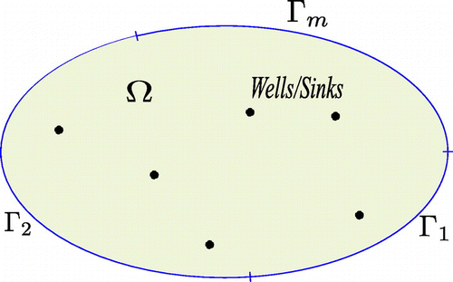
We consider a saturated porous domain $\mathrm{\Omega }$, a bounded domain of ${\mathbb{R}}^2$. We denote by ${\mathrm{\Gamma }}_1$,${\mathrm{\Gamma }}_m$ and ${\mathrm{\Gamma }}_2$ a partition of the boundary $\mathit{\partial }\mathrm{\Omega }$, such that ${\overline{\mathrm{\Gamma }}}_1\cup {\overline{\mathrm{\Gamma }}}_2\cup {\overline{\mathrm{\Gamma }}}_m=\mathit{\partial }\mathrm{\Omega }$. Dirichlet conditions are given on ${\mathrm{\Gamma }}_1$ and ${\mathrm{\Gamma }}_m$ and Neumann condition is given on ${\mathrm{\Gamma }}_2$ as shown in Figure 1. The forward problem is defined by the following incompressible Darcy equations:(1) $$\begin{array}{c}\hfill \left\{\begin{array}{cccc}-\text{div}(T\mathrm{\nabla }h)\hfill & =g(\mathbf{x})\hfill & \hfill & \text{in}\mathrm{\Omega }\hfill \\ h\hfill & =\overline{H}\hfill & \hfill & \text{on}{\mathrm{\Gamma }}_1\hfill \\ T\mathrm{\nabla }h·\mathbf{n}\hfill & =\overline{\mathrm{\Phi }}\hfill & \hfill & \text{on}{\mathrm{\Gamma }}_2\hfill \\ h\hfill & =H\hfill & \hfill & \text{on}{\mathrm{\Gamma }}_m\hfill \end{array}\right.\end{array}$$(1)

where:

• $\mathbf{n}$ is the outward normal on $\mathit{\partial }\mathrm{\Omega }$,

• h is the piezometric head which is the state variable,

• T is the transmissivity parameter. It is a space variable depending function that we can assume constant in an homogeneous isotropic medium, a matrix for an anisotropic homogeneous medium and depends on spatial variables $\mathbf{x}$ for heterogeneous medium,

• $g(\mathbf{x})$ is a linear combination of Dirac distribution representing injection/extraction wells in the domain:

(2) $$\begin{array}{c}\hfill g(\mathbf{x})=\sum _{j=1}^M{\mathit{\lambda }}_j\mathit{\delta }(\mathbf{x}-{\mathbf{P}}_j)\end{array}$$(2)

where M is the well number, $\mathit{\delta }$ is the Dirac operator, ${\mathit{\lambda }}_j\in \mathbb{R}$ and ${\mathbf{P}}_{\mathbf{j}}=(P_{x_j},P_{y_j})$ for $j=1\dots M$ are, respectively, well’s hydraulic flux and location.

Figure 1. Example of domain and its boundary.

Note that in the forward problem defined by Equation (1(1) $$\begin{array}{c}\hfill \left\{\begin{array}{cccc}-\text{div}(T\mathrm{\nabla }h)\hfill & =g(\mathbf{x})\hfill & \hfill & \text{in}\mathrm{\Omega }\hfill \\ h\hfill & =\overline{H}\hfill & \hfill & \text{on}{\mathrm{\Gamma }}_1\hfill \\ T\mathrm{\nabla }h·\mathbf{n}\hfill & =\overline{\mathrm{\Phi }}\hfill & \hfill & \text{on}{\mathrm{\Gamma }}_2\hfill \\ h\hfill & =H\hfill & \hfill & \text{on}{\mathrm{\Gamma }}_m\hfill \end{array}\right.\end{array}$$(1) ), the well’s parameters (${\mathit{\lambda }}_j$, ${\mathbf{P}}_{\mathbf{j}}$, M) and the boundary data ($\overline{H}$, $\overline{\mathrm{\Phi }}$, H) are given, whereas the field h is unknown. In that case, the problem Equation (1(1) $$\begin{array}{c}\hfill \left\{\begin{array}{cccc}-\text{div}(T\mathrm{\nabla }h)\hfill & =g(\mathbf{x})\hfill & \hfill & \text{in}\mathrm{\Omega }\hfill \\ h\hfill & =\overline{H}\hfill & \hfill & \text{on}{\mathrm{\Gamma }}_1\hfill \\ T\mathrm{\nabla }h·\mathbf{n}\hfill & =\overline{\mathrm{\Phi }}\hfill & \hfill & \text{on}{\mathrm{\Gamma }}_2\hfill \\ h\hfill & =H\hfill & \hfill & \text{on}{\mathrm{\Gamma }}_m\hfill \end{array}\right.\end{array}$$(1) ) is well-posed and has a unique solution h in the sense of Hadamard [5].

3. Identification of wells parameters from overspecified boundary data

Consider that the domain $\mathrm{\Omega }$ and the transmissivity T are also given. We assume that an additional condition is given on ${\mathrm{\Gamma }}_m$. So both Dirichlet and Neumann conditions are known on ${\mathrm{\Gamma }}_m$. On the other boundaries ${\mathrm{\Gamma }}_1$ and ${\mathrm{\Gamma }}_2$ Dirichlet and Neumann conditions are given, respectively, as defined in Equation (1(1) $$\begin{array}{c}\hfill \left\{\begin{array}{cccc}-\text{div}(T\mathrm{\nabla }h)\hfill & =g(\mathbf{x})\hfill & \hfill & \text{in}\mathrm{\Omega }\hfill \\ h\hfill & =\overline{H}\hfill & \hfill & \text{on}{\mathrm{\Gamma }}_1\hfill \\ T\mathrm{\nabla }h·\mathbf{n}\hfill & =\overline{\mathrm{\Phi }}\hfill & \hfill & \text{on}{\mathrm{\Gamma }}_2\hfill \\ h\hfill & =H\hfill & \hfill & \text{on}{\mathrm{\Gamma }}_m\hfill \end{array}\right.\end{array}$$(1) ). However, well’s parameters ${\mathit{\lambda }}_j$ and ${\mathbf{P}}_{\mathbf{j}}$ and M are unknown.

3.1. Inverse problem

The considered inverse problem consists in finding well’s parameters ${\mathit{\lambda }}_j$ and ${\mathbf{P}}_{\mathbf{j}}$ and their number M, as defined in Equation (2(2) $$\begin{array}{c}\hfill g(\mathbf{x})=\sum _{j=1}^M{\mathit{\lambda }}_j\mathit{\delta }(\mathbf{x}-{\mathbf{P}}_j)\end{array}$$(2) ), from the knowledge of the overspecified data ($\mathrm{\Phi },H$) on ${\mathrm{\Gamma }}_m$ and the essential and natural boundary data $\overline{H}$ and $\overline{\mathrm{\Phi }}$. It can be defined as follows:

Providing overspecified and compatible data $(H,\mathrm{\Phi })$ on ${\mathrm{\Gamma }}_m$, find the source term $g(\mathbf{x})={\sum }_{j=1}^M{\mathit{\lambda }}_j\mathit{\delta }(\mathbf{x}-{\mathbf{P}}_j)$ such that there exists a field h fulfilling the following system:(3) $$\begin{array}{c}\hfill \left\{\begin{array}{cccc}-\text{div}(T\mathrm{\nabla }h)\hfill & =g(\mathbf{x})\hfill & \hfill & \text{in}\mathrm{\Omega }\hfill \\ h\hfill & =\overline{H}\hfill & \hfill & \text{on}{\mathrm{\Gamma }}_1\hfill \\ T\mathrm{\nabla }h·\mathbf{n}\hfill & =\overline{\mathrm{\Phi }}\hfill & \hfill & \text{on}{\mathrm{\Gamma }}_2\hfill \\ h\hfill & =H\text{and}T\mathrm{\nabla }h·\mathbf{n}=\mathrm{\Phi }\hfill & \hfill & \text{on}{\mathrm{\Gamma }}_m\hfill \end{array}\right.\end{array}$$(3)

with ${\overline{\mathrm{\Gamma }}}_1\cup {\overline{\mathrm{\Gamma }}}_2\cup {\overline{\mathrm{\Gamma }}}_m=\mathit{\partial }\mathrm{\Omega }$.

Identification methods found in the literature require the knowledge of the number of wells to be identified, or at least an upper bound of this number. They are based on the Reciprocity Principle [2], Singular Values Decomposition [6], etc. In this study, we assume that the number M of wells is unknown. Our identification process includes two steps. In the first step, we recover the number of wells and their locations and in the second step we identify their fluxes and so if a well is an injection or an extraction one. The problem is reformulated as a constrained minimization one.

3.2. Minimization problem: the misfit functional and its derivatives

The identification procedure is based on the constitutive law gap functional presented in [4] to solve Cauchy inverse problem, which is inspired from Vogelius’s work [7]. This method was applied in different engineering fields: linear elasticity [8,9], nonlinear elasticity [10], plasticity [11], ElectroCardioGraphy [12], hydrology [1,13], sea intrusion [14], etc.

The principal idea of the method consists in defining two well-posed problems such that everyone uses only one of the overspecified data. These two problems are defined as follows: The first one Equation (4(4) $$\begin{array}{c}\hfill \left\{\begin{array}{cccc}-\text{div}(T\mathrm{\nabla }{h}_D)\hfill & =f(\mathbf{x})\hfill & \hfill & \text{in}\mathrm{\Omega },\hfill \\ h_D\hfill & =\overline{H}\hfill & \hfill & \text{on}{\mathrm{\Gamma }}_1\hfill \\ T\mathrm{\nabla }{h}_D·\mathit{n}\hfill & =\overline{\mathrm{\Phi }}\hfill & \hfill & \text{on}{\mathrm{\Gamma }}_2\hfill \\ h_D\hfill & =H\hfill & \hfill & \text{on}{\mathrm{\Gamma }}_m,\hfill \end{array}\right.\end{array}$$(4) ) is called Dirichlet problem, where the Dirichlet boundary condition on ${\mathrm{\Gamma }}_m$ is used; The second problem Equation (5(5) $$\begin{array}{c}\hfill \left\{\begin{array}{cccc}-\text{div}(T\mathrm{\nabla }{h}_N)\hfill & =f(\mathbf{x})\hfill & \hfill & \text{in}\mathrm{\Omega },\hfill \\ h_N\hfill & =\overline{H}\hfill & \hfill & \text{on}{\mathrm{\Gamma }}_1\hfill \\ T\mathrm{\nabla }{h}_N·\mathbf{n}\hfill & =\overline{\mathrm{\Phi }}\hfill & \hfill & \text{on}{\mathrm{\Gamma }}_2\hfill \\ T\mathrm{\nabla }{h}_N·\mathbf{n}\hfill & =\mathrm{\Phi }\hfill & \hfill & \text{on}{\mathrm{\Gamma }}_m.\hfill \end{array}\right.\end{array}$$(5) ) is called Neumann problem, where the Neumann boundary condition on ${\mathrm{\Gamma }}_m$ is used.(4) $$\begin{array}{c}\hfill \left\{\begin{array}{cccc}-\text{div}(T\mathrm{\nabla }{h}_D)\hfill & =f(\mathbf{x})\hfill & \hfill & \text{in}\mathrm{\Omega },\hfill \\ h_D\hfill & =\overline{H}\hfill & \hfill & \text{on}{\mathrm{\Gamma }}_1\hfill \\ T\mathrm{\nabla }{h}_D·\mathit{n}\hfill & =\overline{\mathrm{\Phi }}\hfill & \hfill & \text{on}{\mathrm{\Gamma }}_2\hfill \\ h_D\hfill & =H\hfill & \hfill & \text{on}{\mathrm{\Gamma }}_m,\hfill \end{array}\right.\end{array}$$(4) (5) $$\begin{array}{c}\hfill \left\{\begin{array}{cccc}-\text{div}(T\mathrm{\nabla }{h}_N)\hfill & =f(\mathbf{x})\hfill & \hfill & \text{in}\mathrm{\Omega },\hfill \\ h_N\hfill & =\overline{H}\hfill & \hfill & \text{on}{\mathrm{\Gamma }}_1\hfill \\ T\mathrm{\nabla }{h}_N·\mathbf{n}\hfill & =\overline{\mathrm{\Phi }}\hfill & \hfill & \text{on}{\mathrm{\Gamma }}_2\hfill \\ T\mathrm{\nabla }{h}_N·\mathbf{n}\hfill & =\mathrm{\Phi }\hfill & \hfill & \text{on}{\mathrm{\Gamma }}_m.\hfill \end{array}\right.\end{array}$$(5)

with $f(\mathbf{x})={\sum }_{j=1}^M{\mathit{\mu }}_j\mathit{\delta }(\mathbf{x}-{\mathbf{Q}}_j)\in \mathbb{R}$ and $(h_D,h_N)\in V_1(\mathrm{\Omega })\times V_2(\mathrm{\Omega })$,$$V_1=\{v\in H^1{(\mathrm{\Omega }),v|}_{{\mathrm{\Gamma }}_1}=\overline{H},v{|}_{{\mathrm{\Gamma }}_m}=H\}\text{and}{V}_2=\{v\in H^1(\mathrm{\Omega }),v{|}_{{\mathrm{\Gamma }}_1}=\overline{H}\}.$$

The fields $h_D$ and $h_N)$ are equal when $f(\mathbf{x})$ meets the real source term $g(\mathbf{x})$ on the domain $\mathrm{\Omega }$, which solves the inverse problem Equation (3(3) $$\begin{array}{c}\hfill \left\{\begin{array}{cccc}-\text{div}(T\mathrm{\nabla }h)\hfill & =g(\mathbf{x})\hfill & \hfill & \text{in}\mathrm{\Omega }\hfill \\ h\hfill & =\overline{H}\hfill & \hfill & \text{on}{\mathrm{\Gamma }}_1\hfill \\ T\mathrm{\nabla }h·\mathbf{n}\hfill & =\overline{\mathrm{\Phi }}\hfill & \hfill & \text{on}{\mathrm{\Gamma }}_2\hfill \\ h\hfill & =H\text{and}T\mathrm{\nabla }h·\mathbf{n}=\mathrm{\Phi }\hfill & \hfill & \text{on}{\mathrm{\Gamma }}_m\hfill \end{array}\right.\end{array}$$(3) ). Therefore, we obtain $h=h_D=h_N$ in $\mathrm{\Omega }$. The idea is to minimize the gap between the two fields $h_D$ and $h_N$ via a misfit function defined as follows:(6) $$\begin{array}{cc}\hfill \mathcal{E}(f(\mathbf{x}))\equiv \mathcal{J}(h_D,h_N)=& \frac{1}{2}{\int }_{\mathrm{\Omega }}T{(\mathrm{\nabla }{h}_D-\mathrm{\nabla }{h}_N)}^T·(\mathrm{\nabla }{h}_D-\mathrm{\nabla }{h}_N)\hfill \\ \hfill & +\frac{a}{2}\left[{\int }_{\mathrm{\Omega }}{(h_D-h^{\text{obs}})}^2+{\int }_{\mathrm{\Omega }}{(h_N-h^{\text{obs}})}^2\right]\hfill \end{array}$$(6)

where $a=1$ if interior measurements in $\mathrm{\Omega }$ are available and $h^{\text{obs}}$ denotes these observations, elsewhere $a=0$. These observations are added in order to improve the identification.

It is straightforward to show that the functional $\mathcal{E}$ is quadratic, positive and hence convex with a minimum equal to zero. Indeed, the quadratic nature of $\mathcal{E}$ is derived from the affine dependence of $h_D$ and $h_N$ to well’s parameters. $\mathcal{E}$ is obviously always positive as $T>0$ and $a=0,1$. It reaches its minimum when $h_D=h_N=h$ , where h is the unique solution to the data recovering problem. The inverse problem Equation (3(3) $$\begin{array}{c}\hfill \left\{\begin{array}{cccc}-\text{div}(T\mathrm{\nabla }h)\hfill & =g(\mathbf{x})\hfill & \hfill & \text{in}\mathrm{\Omega }\hfill \\ h\hfill & =\overline{H}\hfill & \hfill & \text{on}{\mathrm{\Gamma }}_1\hfill \\ T\mathrm{\nabla }h·\mathbf{n}\hfill & =\overline{\mathrm{\Phi }}\hfill & \hfill & \text{on}{\mathrm{\Gamma }}_2\hfill \\ h\hfill & =H\text{and}T\mathrm{\nabla }h·\mathbf{n}=\mathrm{\Phi }\hfill & \hfill & \text{on}{\mathrm{\Gamma }}_m\hfill \end{array}\right.\end{array}$$(3) ) can be formulated as follows:(7) $$\begin{array}{c}\hfill \left\{\begin{array}{cc}\hfill g(\mathbf{x})& =\underset{f(\mathbf{x})\in \mathbb{R}}{argmin}\mathcal{E}(f(\mathbf{x}))\equiv \mathcal{J}(h_D,h_N).\hfill \\ \hfill \text{with:}& \\ \hfill & h_D\text{solution of Equation}\text{(4)},\hfill \\ \hfill & h_N\text{solution of Equation}\text{(5)}.\hfill \end{array}\right.\end{array}$$(7)

To solve the minimization problem Equation (7(7) $$\begin{array}{c}\hfill \left\{\begin{array}{cc}\hfill g(\mathbf{x})& =\underset{f(\mathbf{x})\in \mathbb{R}}{argmin}\mathcal{E}(f(\mathbf{x}))\equiv \mathcal{J}(h_D,h_N).\hfill \\ \hfill \text{with:}& \\ \hfill & h_D\text{solution of Equation}\text{(4)},\hfill \\ \hfill & h_N\text{solution of Equation}\text{(5)}.\hfill \end{array}\right.\end{array}$$(7) ) , we use the adjoint method to compute the functional derivative. We consider the following Lagrangian equation:(8) $$\begin{array}{cc}\hfill \mathcal{L}(h_D,h_N,w_D,w_N,f(\mathbf{x}))& =\frac{1}{2}{\int }_{\mathrm{\Omega }}T{(\mathrm{\nabla }{h}_D-\mathrm{\nabla }{h}_N)}^T·(\mathrm{\nabla }{h}_D-\mathrm{\nabla }{h}_N)\hfill \\ \hfill & +\frac{a}{2}\left[{\int }_{\mathrm{\Omega }}{(h_D-h^{\text{obs}})}^2+{\int }_{\mathrm{\Omega }}{(h_N-h^{\text{obs}})}^2\right]\hfill \\ \hfill & +{\int }_{\mathrm{\Omega }}T\mathrm{\nabla }{h}_D·\mathrm{\nabla }{w}_D+{\int }_{\mathrm{\Omega }}f(\mathbf{x})w_D-{\int }_{{\mathrm{\Gamma }}_2}\overline{\mathrm{\Phi }}{w}_D\hfill \\ \hfill & +{\int }_{\mathrm{\Omega }}T\mathrm{\nabla }{h}_N·\mathrm{\nabla }{w}_N+{\int }_{\mathrm{\Omega }}f(\mathbf{x})w_N-{\int }_{{\mathrm{\Gamma }}_2}\overline{\mathrm{\Phi }}{w}_N-{\int }_{{\mathrm{\Gamma }}_m}\mathrm{\Phi }{w}_N\hfill \end{array}$$(8)

where $(h_D,h_N,w_D,w_N,f(\mathbf{x}))\in V_1(\mathrm{\Omega })\times V_2(\mathrm{\Omega })\times V_1^0\times V_2^0\times \mathbb{R}$ with:$$V_1^0=\{v\in H^1{(\mathrm{\Omega }),v|}_{{\mathrm{\Gamma }}_1}=0,v{|}_{{\mathrm{\Gamma }}_m}=0\}\text{and}{V}_2^0=\{v\in H^1(\mathrm{\Omega }),v{|}_{{\mathrm{\Gamma }}_1}=0\}.$$

and where $w_D$ and $w_N$ are the adjoint fields solution of the following adjoint problems:(9) $$\begin{array}{c}\hfill \left\{\begin{array}{ccc}\hfill -\text{div}(T\mathrm{\nabla }{w}_D)& =a(h_D-h^{\text{obs}})\hfill & \hfill \text{in}\mathrm{\Omega },\\ \hfill w_D& =0\hfill & \hfill \text{on}{\mathrm{\Gamma }}_1\\ \hfill T\mathrm{\nabla }{w}_D·\mathbf{n}& =0\hfill & \hfill \text{on}{\mathrm{\Gamma }}_2\\ \hfill w_D& =0\hfill & \hfill \text{on}{\mathrm{\Gamma }}_m.\\ \hfill \end{array}\right.\\ \hfill \left\{\begin{array}{ccc}\hfill -\text{div}(T\mathrm{\nabla }{w}_N)& =a(h_N-h^{\text{obs}})\hfill & \hfill \text{in}\mathrm{\Omega },\\ \hfill w_N& =0\hfill & \hfill \text{on}{\mathrm{\Gamma }}_1\\ \hfill T\mathrm{\nabla }{w}_N·\mathbf{n}& =0\hfill & \hfill \text{on}{\mathrm{\Gamma }}_2\\ \hfill T\mathrm{\nabla }{w}_N·\mathbf{n}& =T\mathrm{\nabla }{h}_D.\mathbf{n}-\mathrm{\Phi }\hfill & \hfill \text{on}{\mathrm{\Gamma }}_m.\\ \hfill \end{array}\right.\end{array}$$(9)

The derivative of $\mathcal{E}$ can be written as follow:(10) $$\begin{array}{cc}\hfill \mathcal{D}\mathcal{L}·\mathit{\delta }f=\mathcal{D}\mathcal{E}·\mathit{\delta }f& ={\int }_{\mathrm{\Omega }}(w_D+w_N)·\mathit{\delta }f\hfill \end{array}$$(10)

Notice that when $a=0$ the adjoint field $w_D$ vanishes.

3.3. The discrete formulation

The implementation of the above method was carried out using the finite element method (FEM). Hence, the derivative of problem must be established on the basis of the FEM-discretized problem. The advantage of this fully discrete approach is that the exact gradient of the discrete objective function is computed; moreover, it is easily implementable in existing FEM software. We consider a mesh of $\mathrm{\Omega }$ characterized by n nodes and we denote by $p_1$, $p_2$ and $p_m$, respectively, the number of nodes on the boundary ${\mathrm{\Gamma }}_1$, ${\mathrm{\Gamma }}_2$ and ${\mathrm{\Gamma }}_m$.

Remind that, the unknown in this inverse problem is $f(\mathbf{x})$, so we must identify a set of fluxes ${\mathit{\mu }}_j$ and their corresponding locations ${\mathbf{Q}}_{\mathbf{j}}$ for $j=1,M$. Notice that M is also unknown.

In order to avoid to deal with M as a variable, first we assume that each internal node of the FEM mesh could be a well/sink. Consequently, the number of the discretized variable ${\mathit{\mu }}_j$ is equal to that of internal nodes of the mesh. Hereafter, we denote by:

• $X_{\mathit{\mu }}$$\in {\mathbb{R}}^q$, the vector gathering the discretized design variables of $\mathit{\mu }$, with $q=n-p_1-p_2-p_m$,

• $F_{\mathrm{\Phi }}$ and $H_{dis}$$\in {\mathbb{R}}^n$ contain the discretized Neumann and Dirichlet measurements on ${\mathrm{\Gamma }}_m$,

• $H_D$ and $H_N$$\in {\mathbb{R}}^n$ are the discretized fields solution of problems Equation (4(4) $$\begin{array}{c}\hfill \left\{\begin{array}{cccc}-\text{div}(T\mathrm{\nabla }{h}_D)\hfill & =f(\mathbf{x})\hfill & \hfill & \text{in}\mathrm{\Omega },\hfill \\ h_D\hfill & =\overline{H}\hfill & \hfill & \text{on}{\mathrm{\Gamma }}_1\hfill \\ T\mathrm{\nabla }{h}_D·\mathit{n}\hfill & =\overline{\mathrm{\Phi }}\hfill & \hfill & \text{on}{\mathrm{\Gamma }}_2\hfill \\ h_D\hfill & =H\hfill & \hfill & \text{on}{\mathrm{\Gamma }}_m,\hfill \end{array}\right.\end{array}$$(4) ) and Equation (5(5) $$\begin{array}{c}\hfill \left\{\begin{array}{cccc}-\text{div}(T\mathrm{\nabla }{h}_N)\hfill & =f(\mathbf{x})\hfill & \hfill & \text{in}\mathrm{\Omega },\hfill \\ h_N\hfill & =\overline{H}\hfill & \hfill & \text{on}{\mathrm{\Gamma }}_1\hfill \\ T\mathrm{\nabla }{h}_N·\mathbf{n}\hfill & =\overline{\mathrm{\Phi }}\hfill & \hfill & \text{on}{\mathrm{\Gamma }}_2\hfill \\ T\mathrm{\nabla }{h}_N·\mathbf{n}\hfill & =\mathrm{\Phi }\hfill & \hfill & \text{on}{\mathrm{\Gamma }}_m.\hfill \end{array}\right.\end{array}$$(5) ),

• ${\overline{H}}_{dis}$ and $H^{\text{obs}}$$\in {\mathbb{R}}^n$ contain the discretized Dirichlet boundary conditions on ${\mathrm{\Gamma }}_1$ and the interior observations,

• $F_{\overline{\mathrm{\Phi }}}$$\in {\mathbb{R}}^n$ contain the discrete Neumann boundary conditions on ${\mathrm{\Gamma }}_2$

• $L_1$ is $p_1\times n$ matrix and $L_m$ is $p_m\times n$ matrix containing zero and one, they are used to extract from $H_D$ and $H_N$ terms, respectively, on ${\mathrm{\Gamma }}_1$ and ${\mathrm{\Gamma }}_m$,

• $P_{\text{obs}}$ rectangular matrix used to extract terms at the location of the interior measurements, its dimension depends on the number of measurements,

• K is $n\times n$ stiffness matrix.

The discretized forms of problems Equations (4(4) $$\begin{array}{c}\hfill \left\{\begin{array}{cccc}-\text{div}(T\mathrm{\nabla }{h}_D)\hfill & =f(\mathbf{x})\hfill & \hfill & \text{in}\mathrm{\Omega },\hfill \\ h_D\hfill & =\overline{H}\hfill & \hfill & \text{on}{\mathrm{\Gamma }}_1\hfill \\ T\mathrm{\nabla }{h}_D·\mathit{n}\hfill & =\overline{\mathrm{\Phi }}\hfill & \hfill & \text{on}{\mathrm{\Gamma }}_2\hfill \\ h_D\hfill & =H\hfill & \hfill & \text{on}{\mathrm{\Gamma }}_m,\hfill \end{array}\right.\end{array}$$(4) ) and (5(5) $$\begin{array}{c}\hfill \left\{\begin{array}{cccc}-\text{div}(T\mathrm{\nabla }{h}_N)\hfill & =f(\mathbf{x})\hfill & \hfill & \text{in}\mathrm{\Omega },\hfill \\ h_N\hfill & =\overline{H}\hfill & \hfill & \text{on}{\mathrm{\Gamma }}_1\hfill \\ T\mathrm{\nabla }{h}_N·\mathbf{n}\hfill & =\overline{\mathrm{\Phi }}\hfill & \hfill & \text{on}{\mathrm{\Gamma }}_2\hfill \\ T\mathrm{\nabla }{h}_N·\mathbf{n}\hfill & =\mathrm{\Phi }\hfill & \hfill & \text{on}{\mathrm{\Gamma }}_m.\hfill \end{array}\right.\end{array}$$(5) ) are as follows:(11) $$\begin{array}{c}\hfill \left\{\begin{array}{cc}K{H}_D\hfill & =F(X_{\mathit{\mu }})+F_{\overline{\mathrm{\Phi }}}\hfill \\ L_1{H}_D\hfill & ={\overline{H}}_{\text{dis}}\hfill \\ L_m{H}_D\hfill & =H_{\text{dis}}\hfill \end{array}\right.\text{and}\left\{\begin{array}{cc}K{H}_N\hfill & =F(X_{\mathit{\mu }})+F_{\mathrm{\Phi }}+F_{\overline{\mathrm{\Phi }}}\hfill \\ L_1{H}_N\hfill & ={\overline{H}}_{\text{dis}}\hfill \end{array}\right.\end{array}$$(11)

The discrete form of the functional $\mathcal{E}$, defined in Equation (6(6) $$\begin{array}{cc}\hfill \mathcal{E}(f(\mathbf{x}))\equiv \mathcal{J}(h_D,h_N)=& \frac{1}{2}{\int }_{\mathrm{\Omega }}T{(\mathrm{\nabla }{h}_D-\mathrm{\nabla }{h}_N)}^T·(\mathrm{\nabla }{h}_D-\mathrm{\nabla }{h}_N)\hfill \\ \hfill & +\frac{a}{2}\left[{\int }_{\mathrm{\Omega }}{(h_D-h^{\text{obs}})}^2+{\int }_{\mathrm{\Omega }}{(h_N-h^{\text{obs}})}^2\right]\hfill \end{array}$$(6) ), is:(12) $$\begin{array}{c}\hfill E(X_{\mathit{\mu }})=\frac{1}{2}{(H_D-H_N)}^{\top }K(H_D-H_N)+\frac{a}{2}\left[{\left(P_{\text{obs}}{H}_D-H^{\text{obs}}\right)}^2+{\left(P_{\text{obs}}{H}_N-H^{\text{obs}}\right)}^2\right]\end{array}$$(12)

and the discrete form of the functional gradient is:(13) $$\begin{array}{c}\hfill {\mathrm{\nabla }}_{X_{\mathit{\mu }}}E(X_{\mathit{\mu }})=W_D+W_N\end{array}$$(13)

where $W_D$ and $W_N$ are the Lagrange fields solutions of the following problems:(14) $$\begin{array}{cc}& \left\{\begin{array}{cc}K{W}_D\hfill & =K(H_D-H_N)+a{P}_{\text{obs}}^{\top }\left(P_{\text{obs}}{H}_D-H^{\text{obs}}\right)\hfill \\ L_1{W}_D\hfill & =0\hfill \\ L_m{W}_D\hfill & =0\hfill \end{array}\right.\hfill \end{array}$$(14) (15) $$\begin{array}{cc}& \left\{\begin{array}{cc}K{W}_N\hfill & =K(H_N-H_D)+a{P}_{\text{obs}}^{\top }\left(P_{\text{obs}}{H}_N-H^{\text{obs}}\right)\hfill \\ L_1{W}_N\hfill & =0\hfill \end{array}\right.\hfill \end{array}$$(15)

Notice that the method presented in this section allows to recover a distribution of the wells fluxes, the wells positions are recovered as being the coordinates of the points where the hydraulic fluxes reach their local extrema. Therefore, we proceed in two steps:

Step 1

All mesh nodes are considered as possible wells. We minimize the functional E to recover a distribution of well’s fluxes $X_{\mathit{\mu }}^{1\ast }\in {\mathbb{R}}^q$ by solving the following optimization problem:$$X_{\mathit{\mu }}^{1\ast }=arg\underset{X_{\mathit{\mu }}^1}{min}E(X_{\mathit{\mu }}^1)X_{\mathit{\mu }}^1\in {\mathbb{R}}^q$$ Then we extract the local extrema of $X_{\mathit{\mu }}^{1\ast }$. The location of these local extrema are the centres of the wells that we are looking for, consequently the number of injection/extraction wells M is equal to that of the extrema.

Step 2

As the well’s locations are recovered in step 1, in this step we identify the well’s fluxes $X_{\mathit{\mu }}^{2\ast }\in {\mathbb{R}}^M$ at these positions by solving the following optimization problem:$$X_{\mathit{\mu }}^{2\ast }=arg\underset{X_{\mathit{\mu }}^2}{min}E(X_{\mathit{\mu }}^2)X_{\mathit{\mu }}^2\in {\mathbb{R}}^M.$$

The algorithm for wells identification from overspecified boundary data is carried out as described hereafter:

4. Identification of boundary conditions and wells’ parameters from overspecified boundary data

4.1. The inverse problem

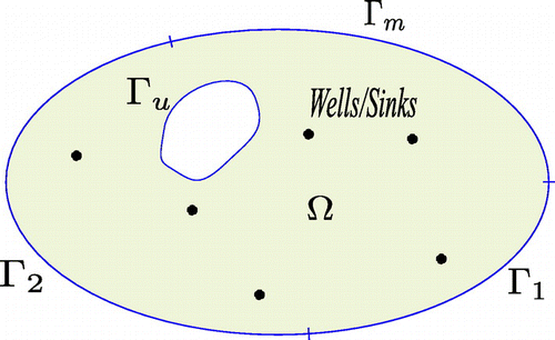
We consider the case where, in addition to well’s parameters, data are missing on an inaccessible part of the domain boundary denoted by ${\mathrm{\Gamma }}_u$, as shown on Figure 2. The aim here is to recover the missing boundary data and well’s parameters ${\mathit{\lambda }}_j$ and ${\mathbf{P}}_{\mathbf{j}}$ and their number M as defined in Equation (2(2) $$\begin{array}{c}\hfill g(\mathbf{x})=\sum _{j=1}^M{\mathit{\lambda }}_j\mathit{\delta }(\mathbf{x}-{\mathbf{P}}_j)\end{array}$$(2) ). Hereafter, we denote by $\mathit{\vartheta }$ and $\mathit{\varphi }$, respectively, the missing Dirichlet and Neumann boundary conditions. As for the first inverse problem studied the preceding section, we assume that an additional condition is given on ${\mathrm{\Gamma }}_m$, and on the other boundaries ${\mathrm{\Gamma }}_1$ and ${\mathrm{\Gamma }}_2$ Dirichlet and Neumann conditions are given, respectively, as defined in Equation (1(1) $$\begin{array}{c}\hfill \left\{\begin{array}{cccc}-\text{div}(T\mathrm{\nabla }h)\hfill & =g(\mathbf{x})\hfill & \hfill & \text{in}\mathrm{\Omega }\hfill \\ h\hfill & =\overline{H}\hfill & \hfill & \text{on}{\mathrm{\Gamma }}_1\hfill \\ T\mathrm{\nabla }h·\mathbf{n}\hfill & =\overline{\mathrm{\Phi }}\hfill & \hfill & \text{on}{\mathrm{\Gamma }}_2\hfill \\ h\hfill & =H\hfill & \hfill & \text{on}{\mathrm{\Gamma }}_m\hfill \end{array}\right.\end{array}$$(1) ). This inverse problem can be formulated as follows:

Providing overspecified and compatible data $(H,\mathrm{\Phi })$, find $(\mathit{\vartheta },\mathit{\varphi },g(\mathbf{x})={\sum }_{j=1}^M{\mathit{\lambda }}_j\mathit{\delta }(\mathbf{x}-{\mathbf{P}}_j))$ such that there exists a field h satisfying the following system:(16) $$\begin{array}{c}\hfill \left\{\begin{array}{cccc}-\text{div}(T\mathrm{\nabla }h)\hfill & =g(\mathbf{x})\hfill & \hfill & \text{in}\mathrm{\Omega }\hfill \\ h\hfill & =\mathit{\vartheta }\text{and}T\mathrm{\nabla }h·\mathbf{n}=\mathit{\phi }\hfill & \hfill & \text{on}{\mathrm{\Gamma }}_u.\hfill \\ h\hfill & =\overline{H}\hfill & \hfill & \text{on}{\mathrm{\Gamma }}_1\hfill \\ T\mathrm{\nabla }h·\mathbf{n}\hfill & =\overline{\mathrm{\Phi }}\hfill & \hfill & \text{on}{\mathrm{\Gamma }}_2\hfill \\ h\hfill & =H\text{and}T\mathrm{\nabla }h·\mathbf{n}=\mathrm{\Phi }\hfill & \hfill & \text{on}{\mathrm{\Gamma }}_m\hfill \end{array}\right.\end{array}$$(16)

with ${\overline{\mathrm{\Gamma }}}_1\cup {\overline{\mathrm{\Gamma }}}_2\cup {\overline{\mathrm{\Gamma }}}_m\cup {\overline{\mathrm{\Gamma }}}_u=\mathit{\partial }\mathrm{\Omega }$.

Figure 2. Example of domain and its boundaries.

In this case, as in the section above, we assume that the number of injection/extraction wells is unknown and we proceed to the resolution of the considered inverse problem, in two steps. In the first step we recover the number of wells/sinks and their locations as well as the missing boundary conditions. Therefore, in the second step we identify their fluxes. The problem is reformulated as a constrained minimization one.

4.2. Minimization problem: the misfit functional and its derivatives

We use the same idea described in Section 3 and define the two following problems as done in [4]. Two well-posed problems are defined as follows: the first one, Dirichlet problem is:(17) $$\begin{array}{c}\hfill \left\{\begin{array}{cccc}-\text{div}(T\mathrm{\nabla }{h}_D)\hfill & =f(\mathbf{x})\hfill & \hfill & \text{in}\mathrm{\Omega },\hfill \\ h_D\hfill & =\overline{H}\hfill & \hfill & \text{on}{\mathrm{\Gamma }}_1\hfill \\ T\mathrm{\nabla }{h}_D·\mathbf{n}\hfill & =\overline{\mathrm{\Phi }}\hfill & \hfill & \text{on}{\mathrm{\Gamma }}_2\hfill \\ h_D\hfill & =H\hfill & \hfill & \text{on}{\mathrm{\Gamma }}_m,\hfill \\ T\mathrm{\nabla }{h}_D·\mathbf{n}\hfill & =\mathit{\eta }\hfill & \hfill & \text{on}{\mathrm{\Gamma }}_u.\hfill \end{array}\right.\end{array}$$(17)

The second one, Neumann problem is:(18) $$\begin{array}{c}\hfill \left\{\begin{array}{cccc}-\text{div}(T\mathrm{\nabla }{h}_N)\hfill & =f(\mathbf{x})\hfill & \hfill & \text{in}\mathrm{\Omega },\hfill \\ h_N\hfill & =\overline{H}\hfill & \hfill & \text{on}{\mathrm{\Gamma }}_1\hfill \\ T\mathrm{\nabla }{h}_N·\mathbf{n}\hfill & =\overline{\mathrm{\Phi }}\hfill & \hfill & \text{on}{\mathrm{\Gamma }}_2\hfill \\ T\mathrm{\nabla }{h}_N·\mathbf{n}\hfill & =\mathrm{\Phi }\hfill & \hfill & \text{on}{\mathrm{\Gamma }}_m.\hfill \\ h_N\hfill & =\mathit{\tau }\hfill & \hfill & \text{on}{\mathrm{\Gamma }}_u,\hfill \end{array}\right.\end{array}$$(18)

with $f(\mathbf{x})={\sum }_{j=1}^M{\mathit{\mu }}_j\mathit{\delta }(\mathbf{x}-{\mathbf{Q}}_j)\in \mathbb{R}$ and $(h_D,h_N)\in V^1(\mathrm{\Omega })\times V^2(\mathrm{\Omega })$,$$V_1=\left\{v\in H^1{(\mathrm{\Omega }),v|}_{{\mathrm{\Gamma }}_1}=\overline{H}{,v|}_{{\mathrm{\Gamma }}_m}=H\}\text{and}{V}_2={\{v\in H^1(\mathrm{\Omega }),v|}_{{\mathrm{\Gamma }}_1}=\overline{H}\right\}$$

The two fields $h_D$ and $h_N$, are equal when all variables $\mathit{\tau }$; $\mathit{\eta }$ and $f(\mathbf{x})$ coincide, respectively, with the corresponding quantities (($\mathit{\vartheta };\mathit{\varphi };g(\mathbf{x})$)) and then the inverse problem Equation (17(17) $$\begin{array}{c}\hfill \left\{\begin{array}{cccc}-\text{div}(T\mathrm{\nabla }{h}_D)\hfill & =f(\mathbf{x})\hfill & \hfill & \text{in}\mathrm{\Omega },\hfill \\ h_D\hfill & =\overline{H}\hfill & \hfill & \text{on}{\mathrm{\Gamma }}_1\hfill \\ T\mathrm{\nabla }{h}_D·\mathbf{n}\hfill & =\overline{\mathrm{\Phi }}\hfill & \hfill & \text{on}{\mathrm{\Gamma }}_2\hfill \\ h_D\hfill & =H\hfill & \hfill & \text{on}{\mathrm{\Gamma }}_m,\hfill \\ T\mathrm{\nabla }{h}_D·\mathbf{n}\hfill & =\mathit{\eta }\hfill & \hfill & \text{on}{\mathrm{\Gamma }}_u.\hfill \end{array}\right.\end{array}$$(17) ) is solved. Therefore, we define a function measuring the gap between the two fields $h_D$ and $h_N$ as done in Section 3:(19) $$\begin{array}{cc}\hfill \mathcal{E}(\mathit{\eta },\mathit{\tau },f(\mathbf{x}))\equiv \mathcal{J}(h_D,h_N)=& \frac{1}{2}{\int }_{\mathrm{\Omega }}T{(\mathrm{\nabla }{h}_D-\mathrm{\nabla }{h}_N)}^T·(\mathrm{\nabla }{h}_D-\mathrm{\nabla }{h}_N)\hfill \\ \hfill & +\frac{a}{2}\left[{\int }_{\mathrm{\Omega }}{\left(h_D-h^{\text{obs}}\right)}^2+{\int }_{\mathrm{\Omega }}{\left(h_N-h^{\text{obs}}\right)}^2\right]\hfill \end{array}$$(19)

The functional $\mathcal{E}$ has the same properties as the previous functional defined in Equation (6(6) $$\begin{array}{cc}\hfill \mathcal{E}(f(\mathbf{x}))\equiv \mathcal{J}(h_D,h_N)=& \frac{1}{2}{\int }_{\mathrm{\Omega }}T{(\mathrm{\nabla }{h}_D-\mathrm{\nabla }{h}_N)}^T·(\mathrm{\nabla }{h}_D-\mathrm{\nabla }{h}_N)\hfill \\ \hfill & +\frac{a}{2}\left[{\int }_{\mathrm{\Omega }}{(h_D-h^{\text{obs}})}^2+{\int }_{\mathrm{\Omega }}{(h_N-h^{\text{obs}})}^2\right]\hfill \end{array}$$(6) ). This inverse problem can be formulated as a constrained optimization one:(20) $$\begin{array}{c}\hfill \left\{\begin{array}{cc}\hfill (\mathit{\vartheta },\mathit{\varphi },g(\mathbf{x}))& =\underset{\mathit{\eta },\mathit{\tau },f(\mathbf{x})}{argmin}\mathcal{E}(f(\mathbf{x}))\equiv \mathcal{J}(h_D,h_N).\hfill \\ \hfill \text{with:}& \\ \hfill & h_D\text{solution of Equation}\text{(18)},\hfill \\ \hfill & h_N\text{solution of Equation}\text{(19)}.\hfill \end{array}\right.\end{array}$$(20)

To solve the minimization problem Equation (21(21) $$\begin{array}{cc}\hfill {\mathrm{\nabla }}_{\mathit{\eta }}\mathcal{E}·\mathit{\delta }\mathit{\eta }& =-{\int }_{{\mathrm{\Gamma }}_u}{v}_D·\mathit{\delta }\mathit{\eta }\hfill \\ \hfill {\mathrm{\nabla }}_{\mathit{\tau }}\mathcal{E}·\mathit{\delta }\mathit{\tau }& =-{\int }_{{\mathrm{\Gamma }}_u}(\mathit{\eta }-T\mathrm{\nabla }{h}_N.\mathbf{n}-T\mathrm{\nabla }{v}_N.\mathbf{n})·\mathit{\delta }\mathit{\tau }\hfill \\ \hfill {\mathrm{\nabla }}_f\mathcal{E}·\mathit{\delta }f& ={\int }_{\mathrm{\Omega }}(v_D+v_N)·\mathit{\delta }f\hfill \end{array}$$(21) ), we have to compute the functional derivatives, which are easily obtained by the adjoint method. The gradient of $\mathcal{E}$ is(21) $$\begin{array}{cc}\hfill {\mathrm{\nabla }}_{\mathit{\eta }}\mathcal{E}·\mathit{\delta }\mathit{\eta }& =-{\int }_{{\mathrm{\Gamma }}_u}{v}_D·\mathit{\delta }\mathit{\eta }\hfill \\ \hfill {\mathrm{\nabla }}_{\mathit{\tau }}\mathcal{E}·\mathit{\delta }\mathit{\tau }& =-{\int }_{{\mathrm{\Gamma }}_u}(\mathit{\eta }-T\mathrm{\nabla }{h}_N.\mathbf{n}-T\mathrm{\nabla }{v}_N.\mathbf{n})·\mathit{\delta }\mathit{\tau }\hfill \\ \hfill {\mathrm{\nabla }}_f\mathcal{E}·\mathit{\delta }f& ={\int }_{\mathrm{\Omega }}(v_D+v_N)·\mathit{\delta }f\hfill \end{array}$$(21)

where $(v_D,v_N)\in V_1^0(\mathrm{\Omega })\times V_2^0(\mathrm{\Omega })$,$$V_1^0=\{v\in H^1{(\mathrm{\Omega }),v|}_{{\mathrm{\Gamma }}_1}{=0,v|}_{{\mathrm{\Gamma }}_m}=0\}\text{and}{V}_2^0=\{v\in H^1{(\mathrm{\Omega }),v|}_{{\mathrm{\Gamma }}_1}=0,v{|}_{{\mathrm{\Gamma }}_u}=0\}$$$(v_D,v_N)$ are, respectively, the adjoint state solution of the two following adjoint problems:(22) $$\begin{array}{cc}& \left\{\begin{array}{ccc}\hfill -\text{div}(T\mathrm{\nabla }{v}_D)& =a(h_D-h^{\text{obs}})\hfill & \hfill \text{in}\mathrm{\Omega },\\ \hfill v_D& =0\hfill & \hfill \text{on}{\mathrm{\Gamma }}_1\\ \hfill T\mathrm{\nabla }{v}_D·\mathbf{n}& =0\hfill & \hfill \text{on}{\mathrm{\Gamma }}_2\\ \hfill v_D& =0\hfill & \hfill \text{on}{\mathrm{\Gamma }}_m,\\ \hfill T\mathrm{\nabla }{v}_D·\mathbf{n}& =T\mathrm{\nabla }{h}_N·\mathit{n}-\mathit{\eta }\hfill & \hfill \text{on}{\mathrm{\Gamma }}_u.\\ \hfill \end{array}\right.\hfill \end{array}$$(22) (23) $$\begin{array}{cc}& \left\{\begin{array}{ccc}\hfill -\text{div}(T\mathrm{\nabla }{v}_N)& =a(h_N-h^{\text{obs}})\hfill & \hfill \text{in}\mathrm{\Omega },\\ \hfill v_N& =0\hfill & \hfill \text{on}{\mathrm{\Gamma }}_1\\ \hfill T\mathrm{\nabla }{v}_N·\mathbf{n}& =0\hfill & \hfill \text{on}{\mathrm{\Gamma }}_2\\ \hfill v_N& =0\hfill & \hfill \text{on}{\mathrm{\Gamma }}_u,\\ \hfill T\mathrm{\nabla }{v}_N·\mathbf{n}& =T\mathrm{\nabla }{h}_D·\mathbf{n}-\mathrm{\Phi }\hfill & \hfill \text{on}{\mathrm{\Gamma }}_m.\\ \hfill \end{array}\right.\hfill \end{array}$$(23)

4.3. The discrete formulation

As in the previous section, the implementation of the above method was carried out using the FEM. Hence, the derivative of problem Equation (22(22) $$\begin{array}{cc}& \left\{\begin{array}{ccc}\hfill -\text{div}(T\mathrm{\nabla }{v}_D)& =a(h_D-h^{\text{obs}})\hfill & \hfill \text{in}\mathrm{\Omega },\\ \hfill v_D& =0\hfill & \hfill \text{on}{\mathrm{\Gamma }}_1\\ \hfill T\mathrm{\nabla }{v}_D·\mathbf{n}& =0\hfill & \hfill \text{on}{\mathrm{\Gamma }}_2\\ \hfill v_D& =0\hfill & \hfill \text{on}{\mathrm{\Gamma }}_m,\\ \hfill T\mathrm{\nabla }{v}_D·\mathbf{n}& =T\mathrm{\nabla }{h}_N·\mathit{n}-\mathit{\eta }\hfill & \hfill \text{on}{\mathrm{\Gamma }}_u.\\ \hfill \end{array}\right.\hfill \end{array}$$(22) ) must be established on the basis of the FEM-discretized problem. We consider a mesh of $\mathrm{\Omega }$ characterized by n nodes and we denote by $p_1$, $p_2$, $p_m$ and $p_u$, respectively, the number of nodes on the boundary ${\mathrm{\Gamma }}_1$, ${\mathrm{\Gamma }}_2$, ${\mathrm{\Gamma }}_m$ and ${\mathrm{\Gamma }}_u$.

Remind that, the unknowns in this inverse problem are the Neumann condition $\mathit{\eta }$ on ${\mathrm{\Gamma }}_u$, the Dirichlet condition $\mathit{\tau }$ on ${\mathrm{\Gamma }}_u$ and $f(\mathbf{x})$. For this latter, we must identify a set of fluxes ${\mathit{\mu }}_j$ and their corresponding locations ${\mathbf{Q}}_{\mathbf{j}}$ for $j=1,M$. Notice that M is also unknown. In order to avoid to deal with M as a variable, first we assume that each internal node of the FEM mesh could be a well/sink. Consequently, the number of the discretized variable ${\mathit{\mu }}_j$ is equal to that of internal nodes of the mesh. Here fter, we denote by:

• $X_{\mathit{\mu }}$$\in {\mathbb{R}}^q$, the vector gathering the discretized variables of $\mathit{\mu }$, with $q=n-p_1-p_2-p_m-p_u$,

• $X_{\mathit{\eta }}$ and $X_{\mathit{\tau }}$ the vectors gathering the discretized variables of $\mathit{\eta }$ and $\mathit{\tau }$ on ${\mathrm{\Gamma }}_u$,

• $F_{\mathrm{\Phi }}$ and $H_{\text{dis}}$$\in {\mathbb{R}}^n$ contain the discretized Neumann and Dirichlet data on ${\mathrm{\Gamma }}_m$,

• $H_D$ and $H_N$$\in {\mathbb{R}}^n$ are the discretized fields solution of problems Equation (18(18) $$\begin{array}{c}\hfill \left\{\begin{array}{cccc}-\text{div}(T\mathrm{\nabla }{h}_N)\hfill & =f(\mathbf{x})\hfill & \hfill & \text{in}\mathrm{\Omega },\hfill \\ h_N\hfill & =\overline{H}\hfill & \hfill & \text{on}{\mathrm{\Gamma }}_1\hfill \\ T\mathrm{\nabla }{h}_N·\mathbf{n}\hfill & =\overline{\mathrm{\Phi }}\hfill & \hfill & \text{on}{\mathrm{\Gamma }}_2\hfill \\ T\mathrm{\nabla }{h}_N·\mathbf{n}\hfill & =\mathrm{\Phi }\hfill & \hfill & \text{on}{\mathrm{\Gamma }}_m.\hfill \\ h_N\hfill & =\mathit{\tau }\hfill & \hfill & \text{on}{\mathrm{\Gamma }}_u,\hfill \end{array}\right.\end{array}$$(18) ) and Equation (19(19) $$\begin{array}{cc}\hfill \mathcal{E}(\mathit{\eta },\mathit{\tau },f(\mathbf{x}))\equiv \mathcal{J}(h_D,h_N)=& \frac{1}{2}{\int }_{\mathrm{\Omega }}T{(\mathrm{\nabla }{h}_D-\mathrm{\nabla }{h}_N)}^T·(\mathrm{\nabla }{h}_D-\mathrm{\nabla }{h}_N)\hfill \\ \hfill & +\frac{a}{2}\left[{\int }_{\mathrm{\Omega }}{\left(h_D-h^{\text{obs}}\right)}^2+{\int }_{\mathrm{\Omega }}{\left(h_N-h^{\text{obs}}\right)}^2\right]\hfill \end{array}$$(19) ),

• ${\overline{H}}_{\text{dis}}$ and $H^{\text{obs}}$$\in {\mathbb{R}}^n$ contain the discretized Dirichlet boundary conditions on ${\mathrm{\Gamma }}_1$ and the interior observations,

• $F_{\overline{\mathrm{\Phi }}}$$\in {\mathbb{R}}^n$ contain the discrete Neumann boundary conditions on ${\mathrm{\Gamma }}_2$

• $L_1$ is $p_1\times n$ matrix, $L_u$ is $p_u\times n$ matrix and $L_m$ is $p_m\times n$ matrix containing zero and one, they are used to extract from $H_D$ and $H_N$ terms, respectively, on ${\mathrm{\Gamma }}_1$, ${\mathrm{\Gamma }}_u$ and ${\mathrm{\Gamma }}_m$,

• $P_{\text{obs}}$ rectangular matrix used to extract terms at the location of the interior measurements, its dimension depends on the number of measurements,

• K is $n\times n$ stiffness matrix.

The discretized forms of problems Equations (18(18) $$\begin{array}{c}\hfill \left\{\begin{array}{cccc}-\text{div}(T\mathrm{\nabla }{h}_N)\hfill & =f(\mathbf{x})\hfill & \hfill & \text{in}\mathrm{\Omega },\hfill \\ h_N\hfill & =\overline{H}\hfill & \hfill & \text{on}{\mathrm{\Gamma }}_1\hfill \\ T\mathrm{\nabla }{h}_N·\mathbf{n}\hfill & =\overline{\mathrm{\Phi }}\hfill & \hfill & \text{on}{\mathrm{\Gamma }}_2\hfill \\ T\mathrm{\nabla }{h}_N·\mathbf{n}\hfill & =\mathrm{\Phi }\hfill & \hfill & \text{on}{\mathrm{\Gamma }}_m.\hfill \\ h_N\hfill & =\mathit{\tau }\hfill & \hfill & \text{on}{\mathrm{\Gamma }}_u,\hfill \end{array}\right.\end{array}$$(18) ) and (19(19) $$\begin{array}{cc}\hfill \mathcal{E}(\mathit{\eta },\mathit{\tau },f(\mathbf{x}))\equiv \mathcal{J}(h_D,h_N)=& \frac{1}{2}{\int }_{\mathrm{\Omega }}T{(\mathrm{\nabla }{h}_D-\mathrm{\nabla }{h}_N)}^T·(\mathrm{\nabla }{h}_D-\mathrm{\nabla }{h}_N)\hfill \\ \hfill & +\frac{a}{2}\left[{\int }_{\mathrm{\Omega }}{\left(h_D-h^{\text{obs}}\right)}^2+{\int }_{\mathrm{\Omega }}{\left(h_N-h^{\text{obs}}\right)}^2\right]\hfill \end{array}$$(19) ) are, respectively:(24) $$\begin{array}{c}\hfill \left\{\begin{array}{cc}K{H}_D\hfill & =F(X_{\mathit{\mu }},X_{\mathit{\eta }})+F_{\overline{\mathrm{\Phi }}}\hfill \\ L_1{H}_D\hfill & ={\overline{H}}_{\text{dis}}\hfill \\ L_m{H}_D\hfill & =H_{\text{dis}}\hfill \end{array}\right.\text{and}\left\{\begin{array}{cc}K{H}_N\hfill & =F(X_{\mathit{\mu }})+F_{\mathrm{\Phi }}+F_{\overline{\mathrm{\Phi }}}\hfill \\ L_1{H}_N\hfill & ={\overline{H}}_{\text{dis}}\hfill \\ L_u{H}_N\hfill & =X_{\mathit{\tau }}\hfill \end{array}\right.\end{array}$$(24)

The discrete form of the functional $\mathcal{J}$ is:(25) $$\begin{array}{c}\hfill J(X_{\mathit{\eta }},X_{\mathit{\tau }},X_{\mathit{\mu }})=\frac{1}{2}{(H_D-H_N)}^{\top }K(H_D-H_N)+\frac{a}{2}\left[{(P_{\text{obs}}{H}_D-H^{\text{obs}})}^2+{(P_{\text{obs}}{H}_N-H^{\text{obs}})}^2\right]\end{array}$$(25)

and the discrete form of the gradient functional is:(26) $$\begin{array}{c}\hfill \mathrm{\nabla }J(X_{\mathit{\eta }},X_{\mathit{\tau }},X_{\mathit{\mu }})=\left[\begin{array}{c}{L}_u{\mathit{\lambda }}_D\\ L_u(K(H_N-H_D)-K{\mathit{\lambda }}_N)\\ {\mathit{\lambda }}_D+{\mathit{\lambda }}_N\end{array}\right]\end{array}$$(26)

where ${\mathit{\lambda }}_D$ and ${\mathit{\lambda }}_N$ are the Lagrange multipliers solution of the following problems:(27) $$\begin{array}{c}\hfill \left\{\begin{array}{cc}K{\mathit{\lambda }}_D\hfill & =K(H_D-H_N)+a{P}_{\text{obs}}^{\top }(P_{\text{obs}}{H}_D-H^{\text{obs}})\hfill \\ L_1{\mathit{\lambda }}_D\hfill & =0\hfill \\ L_m{\mathit{\lambda }}_D\hfill & =0\hfill \end{array}\right.\end{array}$$(27) (28) $$\begin{array}{c}\hfill \left\{\begin{array}{cc}K{\mathit{\lambda }}_N\hfill & =K(H_N-H_D)+a{P}_{\text{obs}}^{\top }(P_{\text{obs}}{H}_N-H^{\text{obs}})\hfill \\ L_1{\mathit{\lambda }}_N\hfill & =0\hfill \\ L_u{\mathit{\lambda }}_N\hfill & =0\hfill \end{array}\right.\end{array}$$(28)

To solve the inverse problem Equation (17(17) $$\begin{array}{c}\hfill \left\{\begin{array}{cccc}-\text{div}(T\mathrm{\nabla }{h}_D)\hfill & =f(\mathbf{x})\hfill & \hfill & \text{in}\mathrm{\Omega },\hfill \\ h_D\hfill & =\overline{H}\hfill & \hfill & \text{on}{\mathrm{\Gamma }}_1\hfill \\ T\mathrm{\nabla }{h}_D·\mathbf{n}\hfill & =\overline{\mathrm{\Phi }}\hfill & \hfill & \text{on}{\mathrm{\Gamma }}_2\hfill \\ h_D\hfill & =H\hfill & \hfill & \text{on}{\mathrm{\Gamma }}_m,\hfill \\ T\mathrm{\nabla }{h}_D·\mathbf{n}\hfill & =\mathit{\eta }\hfill & \hfill & \text{on}{\mathrm{\Gamma }}_u.\hfill \end{array}\right.\end{array}$$(17) ) we proceed in two steps as in the previous section.

Step 1

The identification of the missing boundary data ($X_{\mathit{\eta }}^{\ast },X_{\mathit{\tau }}^{\ast }$) and wells’ flows $X_{\mathit{\mu }}^{1\ast }$ is carried out simultaneously by solving the following optimization problem:$$(X_{\mathit{\eta }}^{\ast },X_{\mathit{\tau }}^{\ast },X_{\mathit{\mu }}^{1\ast })=arg\underset{X_{\mathit{\eta }},X_{\mathit{\tau }},X_{\mathit{\mu }}^1}{min}J(X_{\mathit{\eta }},X_{\mathit{\tau }},X_{\mathit{\mu }}^1)(X_{\mathit{\eta }},X_{\mathit{\tau }},X_{\mathit{\mu }}^1)\in {\mathbb{R}}^{p_u}\times {\mathbb{R}}^{p_u}\times {\mathbb{R}}^q$$ Then local extrema of $X_{\mathit{\mu }}^{1\ast }$ are extracted and their positions are the centres of the sought wells, consequently the number of wells M is equal to that of the extrema.

Step 2

As all boundary conditions and the number of wells were recovered, the identification of the corresponding M flows $X_{\mathit{\mu }}^{2\ast }$ is carried out by solving the following optimization problem:$$X_{\mathit{\mu }}^{2\ast }=arg\underset{X_{\mathit{\mu }}^2}{min}J(X_{\mathit{\eta }}^{\ast },X_{\mathit{\tau }}^{\ast },X_{\mathit{\mu }}^2)X_{\mathit{\mu }}^2\in {\mathbb{R}}^M$$

The algorithm for wells/sinks and boundary data identification from overspecified boundary data is carried out as described hereafter:

5. Numerical experiments

To test the efficiency of the proposed reconstruction process, different cases are carried out using the FEM. All the computations have been run on Comsol Multiphysics.[15] We define the relative errors as:(29) $$\begin{array}{c}\hfill {\mathit{ϵ}}_P=100\left|\frac{\Vert {\overrightarrow{OP}}_{ex}{\Vert }_2-{\Vert {\overrightarrow{OP}}_{id}\Vert }_2}{\Vert {\overrightarrow{OP}}_{ex}{\Vert }_2}\right|\end{array}$$(29)

for position’s identification and:(30) $$\begin{array}{c}\hfill {\mathit{ϵ}}_Q=100\left|\frac{Q_{ex}-Q_{id}}{Q_{ex}}\right|\end{array}$$(30)

for fluxes’ identification. where subscripts ‘ex’ and ‘id’ denote exact and identified; Q denotes the flux; O denotes the origin of the coordinate system and P denotes a well’s position. Subscripts ex and id denote exact and identified values.

5.1. Injection/extraction wells identification from overspecified boundary data

In this example, numerical trials are performed on a rectangular domain of $20\times 10{\text{km}}^2$, the transmissivity of the medium is $T=0.001{\text{m}}^2{\text{s}}^{-1}$. Vertical boundaries are considered impermeable ($\overline{\mathrm{\Phi }}=0$), the Dirichlet condition on the upper horizontal boundary is $\overline{H}=40m$ and the measurement data on the lower horizontal boundary is $H=90m$. The overspecified data were extracted from the exact solution h(x, y) of the forward problem given by equation Equation (1(1) $$\begin{array}{c}\hfill \left\{\begin{array}{cccc}-\text{div}(T\mathrm{\nabla }h)\hfill & =g(\mathbf{x})\hfill & \hfill & \text{in}\mathrm{\Omega }\hfill \\ h\hfill & =\overline{H}\hfill & \hfill & \text{on}{\mathrm{\Gamma }}_1\hfill \\ T\mathrm{\nabla }h·\mathbf{n}\hfill & =\overline{\mathrm{\Phi }}\hfill & \hfill & \text{on}{\mathrm{\Gamma }}_2\hfill \\ h\hfill & =H\hfill & \hfill & \text{on}{\mathrm{\Gamma }}_m\hfill \end{array}\right.\end{array}$$(1) ) with given point sources coordinates $(x_k,y_k)$ and intensities $Q_k$. The domain is meshed with linear triangular elements: 735 nodes and 1366 elements. Different cases were studied and commented hereafter:

(A)	Sensitivity to measurements: we consider two situations, in the first one only overspecified boundary data are available ($a=0$) and in the second one additional data (fluxes at interior positions of the domain) are available ($a=1$). Table 1 shows identified values of wells fluxes and their locations, they are compared to the exact values. As expected, the identification process is improved when additional data are used.
(B)	Multiple wells case: We consider in this case a set of five wells with positive and negative fluxes. The corresponding exact hydraulic head distribution is represented in Figure 3(a). As shown in Figure 3(b) exact and recovered wells are very closed. This remark is confirmed in Table 2 in which exact and identified wells’ locations, their corresponding fluxes and relative errors are shown. We observe a good agreement between exact and identified values with relative errors within $5\%$.
(C)	Sensitivity to noisy data: In practical situations, measurements are usually polluted by uncertainties, which are often due to measuring instrument, to the item to be measured, to the environment, to the operator and to many other sources. In our studies, noisy data were generated by adding a Gaussian white noise distribution to Dirichlet data on ${\mathrm{\Gamma }}_m$. Table 3 gathers exact and identified values as well as relative errors for different noise levels varying from 2 to 8%. Notice here that relative errors remain less than $9\%$ for locations values, whereas for fluxes values it is higher but remain under $15\%$ for fluxes ones. This difference could be explained by the fact that fluxes were identified in a second step after the identification of their locations, consequently the errors on locations are propagated to the fluxes values.
(D)	Sensitivity to the relative position: It is known that when wells to be recovered are close to each other, they interact through their influence cones, therefore it is important to study the influence of the distance between wells in the identification process. We consider the case with only two wells separated by a distance d varying from $16m$ to $2m$ with fluxes $Q_1=100m^3/s$ and $Q_2=50m^3/s$. We computed the relative errors on recovered fluxes and locations for each distance value. Table 4 shows exact, identified and highest relative errors obtained for four cases. As expected, one can observe in Table 4 that if the wells are well separated (enough far from each other), the fluxes and the positions are in a good agreement the exact values as the relative errors remain within $5\%$, whereas when the distance between the wells decreases sufficiently (less than $4m$), the identification becomes less accurate as relative errors increase and are around $10\%$.

Figure 3. Identified hydraulic head distribution and wells’ positions for the rectangular example.

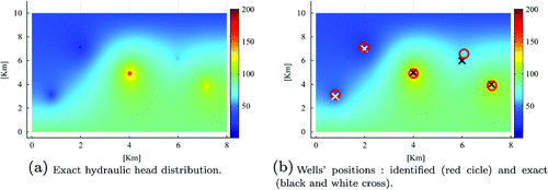
Table 1. Exact and identified wells’ fluxes and their locations compared to exact values without interior observations.

Exact data	$P_{ex}(\mathrm{m})$	(2500, 1000)	(4500, 3500)	(7000, 1500)	(1500, 4000)
	$Q_{ex}({10}^{-3}{\mathrm{m}}^3/\mathrm{s})$	$-60$	80	$-60$	$-40$
$a=0$	$P_{id}(\mathrm{m})$	(2580, 1100)	(4610, 3640)	(6900, 1610)	(1800, 4200)
	${\mathit{ϵ}}_P(\%)$	4.16	3.03	1.03	6.96
	$Q_{id}({10}^{-3}{\mathrm{m}}^3/\mathrm{s})$	$-56.6$	75.1	$-54.1$	$-35.2$
	${\mathit{ϵ}}_Q(\%)$	5.66	6.12	9.8	12
$a=1$	$P_{id}(\mathrm{m})$	(2500, 1080)	(4480, 3760)	(6900, 1660)	(1450, 3900)
	${\mathit{ϵ}}_P(\%)$	1.14	2.59	0.86	2.60
	$Q_{id}({10}^{-3}{\mathrm{m}}^3/\mathrm{s})$	$-56.9$	76.8	$-55.5$	$-37.9$
	${\mathit{ϵ}}_Q(\%)$	5.1	4	7.5	5.25

Table 2. Identified data compared to exact values in the case of five wells with interiors observations ($a=1$).

Wells	$P_1$	$P_2$	$P_3$	$P_4$	$P_5$
$P_{ex}(\mathrm{m})$	(2000, 3000)	(5000, 7000)	(10000, 5000)	(15000, 6000)	(18000, 4000)
$Q_{ex}({10}^{-3}{\mathrm{m}}^3/\mathrm{s})$	$-50$	$-70$	150	$-30$	80
$P_{id}(\mathrm{m})$	(1982, 3130)	(4950, 7128)	(10000, 4920)	(15220, 6570)	(18080, 3873)
${\mathit{ϵ}}_P(\%)$	2.75	0.88	0.31	2.61	0.27
$Q_{id}({10}^{-3}{\mathrm{m}}^3/\mathrm{s})$	$-52$	$-68.7$	147.9	$-28.8$	78.9
${\mathit{ϵ}}_Q(\%)$	4	1.85	1.4	4	1.37

Table 3. Identified data compared to exact values for different noise level in the case of five wells.

$Noiselevel(\%)$	2	4	6	8
$P_{id}^1(\mathrm{m})$	(1845, 3142)	(1831, 3710)	(1803, 3183)	(1789, 3198)
${\mathit{ϵ}}_P(\%)$	1.05	2.50	1.46	1.63
$Q_{id}^1({10}^{-3}{\mathrm{m}}^3/\mathrm{s})$	$-52.8$	$-53.3$	$-53.9$	$-54.3$
${\mathit{ϵ}}_Q(\%)$	5.6	6.6	7.8	8.6
$P_{id}^2(\mathrm{m})$	(4699, 7017)	(4631, 6983)	(4613, 6971)	(4596, 6936)
${\mathit{ϵ}}_P(\%)$	1.83	2.60	2.82	3.27
$Q_{id}^2({10}^{-3}{\mathrm{m}}^3/\mathrm{s})$	$-67.8$	$-66.1$	$-65.6$	64.2
${\mathit{ϵ}}_Q(\%)$	3.14	5.57	6.28	8.2
$P_{id}^3(\mathrm{m})$	(10080, 4857)	(9950, 4830)	(9859, 4803)	(9801, 4790)
${\mathit{ϵ}}_P(\%)$	0.07	1.07	1.91	2.42
$Q_{id}^3({10}^{-3}{\mathrm{m}}^3/\mathrm{s})$	146.5	144.6	143.5	141.5
${\mathit{ϵ}}_Q(\%)$	2.33	3.6	4.33	5.66
$P_{id}^4(\mathrm{m})$	(15340, 5840)	(15896, 5685)	(16235, 5780)	(16310, 5735)
${\mathit{ϵ}}_P(\%)$	1.6	4.49	6.676	7.01
$Q_{id}^4({10}^{-3}{\mathrm{m}}^3/\mathrm{s})$	$-28$	$-27.4$	$-33.2$	$-34.2$
${\mathit{ϵ}}_Q(\%)$	6.66	8.66	10.66	14
$P_{id}^5(\mathrm{m})$	(18180, 4040)	(18320, 3964)	(18398, 3908)	(18420, 3832)
${\mathit{ϵ}}_P(\%)$	1.00	1.65	2.00	2.03
$Q_{id}^5({10}^{-3}{\mathrm{m}}^3/\mathrm{s})$	78	77.3	3.87	75.9
${\mathit{ϵ}}_Q(\%)$	2.5	3.37	3.87	5.12

Table 4. Identified data compared to exact values in the case of 2 wells separated by different distances d.

d (km)	16	8	4	2
$P_{ex}^1(\mathrm{m})$	(2000, 5000)	(4000, 5000)	(4000, 5000)	(6000, 5000)
$P_{id}^1(\mathrm{m})$	(1923, 5071)	(4080, 5196)	(4210, 5208)	(6680, 5296)
$P_{ex}^2(\mathrm{m})$	(18000, 5000)	(12000, 5000)	(8000, 5000)	(8000, 5000)
$P_{id}^2(\mathrm{m})$	(18008, 5052)	(12021, 5087)	(8310, 5263)	(7068, 5390)
${\mathit{ϵ}}_P(\%)$	0.71	3.17	4.58	9.14
$Q_{id}^1({\mathrm{m}}^3/\mathrm{s})$	99.92	99.56	95.36	87.12
${\mathit{ϵ}}_Q(\%)$	0.08	0.44	4.64	12.88
$Q_{id}^2({\mathrm{m}}^3/\mathrm{s})$	50.02	50.15	53.2	57.08
${\mathit{ϵ}}_Q(\%)$	0.04	0.3	6.4	14.16

5.2. Boundary data and wells’ identification from overspecified boundary data

In order to check the methodology with an hydrogeologic configuration, we consider the Rocky Mountain Arsenal example based on the detailed model in [16]. We took the simplified idealization studied as a test case in SUTRA code developed by Voss in [17]. The porous media is supposed isotropic and heterogeneous. Figure 4(a) shows the geometry and boundary conditions data. The domain is $6100\times 4880m^2$ heterogeneous rectangle with a porosity $\mathit{\omega }=0.2$, a constant transmissivity $T_1=2.5{10}^{-4}{m}^2/s$ and two impermeable bedrock outcrops represented by two rectangles with relative low transmissivities $T_2=T_3=2.5{10}^{-8}{m}^2/s$.

Figure 4. Domain geometry, boundaries and interior observations.

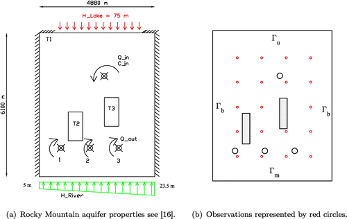
Figure 5. Recovered boundary data on ${\mathrm{\Gamma }}_u$ from overspecified data and 20 interior observations for the Rocky mountain aquifer.

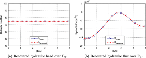
Figure 6. Recovered boundary data on ${\mathrm{\Gamma }}_u$ for different noise level in the Rocky Mountain aquifer.

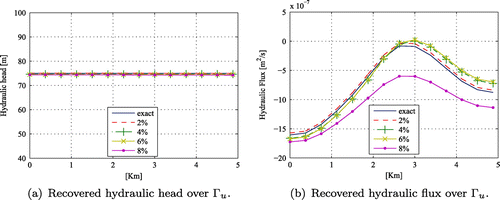
Table 5. Identified data compared to exact values using overspecified boundary data and additional 20 interior observations in the case of Rocky Mountain aquifer. Given data are noise-free.

Wells	$P_1$	$P_2$	$P_3$	$P_4$
$P_{ex}(\mathrm{m})$	(915, 1220)	(2135, 1220)	(3355, 1220)	2747, 4270)
$Q_{ex}({10}^{-3}{\mathrm{m}}^3/\mathrm{s})$	$-0.5$	$-0.5$	$-0.5$	1.8
$P_{id}(\mathrm{m})$	(885, 1195)	(2096, 1197)	(3398, 1190)	2637, 4241)
${\mathit{ϵ}}_P(\%)$	3.05	2.91	1.21	2.86
$Q_{id}({10}^{-3}{\mathrm{m}}^3/\mathrm{s})$	$-0.494$	$-0.492$	$-0.492$	1.82
${\mathit{ϵ}}_Q(\%))$	1.2	1.8	1.6	0.01

Table 6. Identified data compared to exact values for different noise level in the case of Rocky Mountain aquifer. Given data are noisy.

$Noiselevel(\%)$	2	4	6	8
$P_{id}^1(\mathrm{m})$	(880, 1188)	(872, 1173)	(927, 1141)	(935, 1130)
${\mathit{ϵ}}_P\%)$	3.05	4.15	3.60	3.82
$Q_{id}^1({10}^{-3}{\mathrm{m}}^3/\mathrm{s})$	$-0.0487$	$-0.0480$	$-0.0472$	0.0450
${\mathit{ϵ}}_Q(\%)$	2.5	4	5.6	10
$P_{id}^2(\mathrm{m})$	(2189, 1270)	(2185, 1291)	(2078, 1118)	(2070, 1102)
${\mathit{ϵ}}_P(\%)$	2.91	3.21	4.04	4.63
$Q_{id}^2({10}^{-3}{\mathrm{m}}^3/\mathrm{s})$	$-0.0486$	$-0.0481$	$-0.0474$	0.0452
${\mathit{ϵ}}_Q(\%)$	2.8	3.8	5.2	9.6
$P_{id}^3(\mathrm{m})$	(3415, 1180)	(3270, 1161)	(3258, 1115)	(3242, 1109)
${\mathit{ϵ}}_P(\%)$	1.21	2.80	3.54	4.02
$Q_{id}^3({10}^{-3}{\mathrm{m}}^3/\mathrm{s})$	$-0.0488$	$-0.0485$	$-0.048$	0.0466
${\mathit{ϵ}}_Q(\%)$	2.4	3	4	6.8
$P_{id}^4(\mathrm{m})$	(2812, 4401)	(2818, 4429)	(2823, 4469)	(2831, 4469)
${\mathit{ϵ}}_P(\%)$	2.86	3.90	4.02	4.20
$Q_{id}^4({10}^{-3}{\mathrm{m}}^3/\mathrm{s})$	0.177	0.174	0.171	0.168
${\mathit{ϵ}}_Q(\%)$	1.6	3.3	5	6.6

The aquifer is bounded by a lake at the north with a constant piezometric head $h_n=75m$ and a river at the south with linear piezometric head, varying from $5m$ to $23.5m$ and two impervious lateral borders. Theses boundaries are, respectively, denoted by ${\mathrm{\Gamma }}_u$, ${\mathrm{\Gamma }}_m$ and ${\mathrm{\Gamma }}_b$ (see Figure 4(a)). The aquifer is exploited by three wells (1, 2 and 3) pumping at a rate of $Q_{out}^1=-0.5{10}^{-3}{m}^3/s$ each. A contamination enters the system through a leaking waste isolation pond situated in the north at ($2745m,4270m$) with a constant rate of $Q_{in}^4=1.8{10}^{-3}{m}^3/s$. Table 5 summarizes wells’ positions and rates. The forward problem is solved using a linear triangular finite element mesh characterized by 499 nodes and 921 elements. The resulting fields were used to extract overspecified data which were used to solve the inverse problem.

The inverse problem dealt with here is formulated as follows, we consider that:

(1)	at the boundary ${\mathrm{\Gamma }}_m$ overspecified data are available (fluxes and piezometric head),
(2)	at the top boundary ${\mathrm{\Gamma }}_u$ data are unknown (fluxes and piezometric head),
(3)	in addition, we consider that for the four wells’ positions and fluxes are also unknown.

We assume that some local observations, 20 piezometric head measurements, are available as shown in Figure 4(b). These 20 interior measurements points represent 4$\%$ of the total mesh nodes (499). Their positions are chosen by taking one measurement on each 25 mesh nodes.

The identification procedure is based on the algorithm 2(2) $$\begin{array}{c}\hfill g(\mathbf{x})=\sum _{j=1}^M{\mathit{\lambda }}_j\mathit{\delta }(\mathbf{x}-{\mathbf{P}}_j)\end{array}$$(2) . In the first step, the missing boundary data on ${\mathrm{\Gamma }}_u$ and the wells’ coordinates positions were identified. Figure 5(a) and (b) show the distribution of the identified piezometric head and flux on ${\mathrm{\Gamma }}_u$ using noise-free data. We observe a good accuracy in comparison to the exact values of the forward problem. Table 5 shows the identified coordinates for each well compared to the exact ones. Notice that the relative errors are less than $3.05\%$. In the second step, using the recovered boundary data on ${\mathrm{\Gamma }}_u$ with the above given data, we identify the resulting flows associated with the previously identified wells’ positions. Table 5 shows also the identified flow values compared to exact ones with relatives errors less than $2\%$.

In real cases, given data are often measured and so they are noisy. In order to take into account the effect of noise on the identified values, we introduce an additive noise on ${\mathrm{\Gamma }}_m$ by adding $a\%$ of artificial Gaussian white noise. Figure 6(a) and (b) show the identified flux and hydraulic head on ${\mathrm{\Gamma }}_u$ for different noise level $a\%$. Notice that the noise effect is more important on the identified flux. Nevertheless the identified values remain satisfactory for reasonable noise level less than $6\%$. Table 6 shows the identified coordinates and flows of the four wells for different noise level. The relative errors remain less that $6\%$ for reasonable noise level less than $6\%$ and increase beyond this level.

6. Conclusion

The management of water resources is a problem of great importance. The goal is to find a reasonable balance between these resources and demand while preserving the quality of water. Towards this goal it is essential to identify sources and sinks in the studied porous media since an important number of wells could be illegal and/or badly exploited.

For these purposes, we developed an identification methodology based on different identification algorithms exploiting overspecified boundary data. We dealt with two inverse problems. In the first problem, we assumed that all boundary data are given and on a part of the boundary overspecified data are available. In this case, only well’s parameters were considered unknown. In the second inverse problem, we assumed that boundary data and overspecified data are given only on a part of the boundary, whereas on the remaining part data are missing. In this latter case, well’s parameters and boundary data were considered unknown. The involved algorithms rely on the minimization of a constitutive law gap functional already studied in [4] and extended here to source parameters identification. For hard cases, such difficulties in distinguishing different neighbouring wells, additional data taken inside the domain, for instance measured piezometric heads, could be easily used in the procedure. With this additional data, we observed a substantial improvement in the identification results.

The presented identification process of wells’ positions and flows from complete/incomplete overspecified boundary data seems to be efficient and promising according to the numerical examples dealt with. Forthcoming publications will deal with real applications and measured data where regularization techniques will be involved in order to control noise effect and to proof the robustness of the proposed methodology.

Acknowledgements

The Partenariat Hubert Curien – Utique program is acknowledged for its financial funding through the project indexed 14G1103, as well as the Euro – Mediterranean $3+3$ program through the project 12/MED/03 (Hydrinv).

Additional information

Funding

This work was supported by Partenariat Hubert Curien – Utique program project indexed [14G1103]; Euro – Mediterranean $3+3$ program through the project [12/MED/03] (Hydrinv).

Notes

No potential conflict of interest was reported by the authors.

Appendix 1

Lagrangian derivative: adjoint states

The components of the gradient can be computed in a more efficient way using the adjoint state method, which makes it possible to evaluate the gradient in any direction using only the determination of two adjoint fields $w_D$ and $w_N$.

We consider the Lagrangian done by Equation (8(8) $$\begin{array}{cc}\hfill \mathcal{L}(h_D,h_N,w_D,w_N,f(\mathbf{x}))& =\frac{1}{2}{\int }_{\mathrm{\Omega }}T{(\mathrm{\nabla }{h}_D-\mathrm{\nabla }{h}_N)}^T·(\mathrm{\nabla }{h}_D-\mathrm{\nabla }{h}_N)\hfill \\ \hfill & +\frac{a}{2}\left[{\int }_{\mathrm{\Omega }}{(h_D-h^{\text{obs}})}^2+{\int }_{\mathrm{\Omega }}{(h_N-h^{\text{obs}})}^2\right]\hfill \\ \hfill & +{\int }_{\mathrm{\Omega }}T\mathrm{\nabla }{h}_D·\mathrm{\nabla }{w}_D+{\int }_{\mathrm{\Omega }}f(\mathbf{x})w_D-{\int }_{{\mathrm{\Gamma }}_2}\overline{\mathrm{\Phi }}{w}_D\hfill \\ \hfill & +{\int }_{\mathrm{\Omega }}T\mathrm{\nabla }{h}_N·\mathrm{\nabla }{w}_N+{\int }_{\mathrm{\Omega }}f(\mathbf{x})w_N-{\int }_{{\mathrm{\Gamma }}_2}\overline{\mathrm{\Phi }}{w}_N-{\int }_{{\mathrm{\Gamma }}_m}\mathrm{\Phi }{w}_N\hfill \end{array}$$(8) ):$$\begin{array}{cc}\hfill \mathcal{L}(h_D,h_N,w_D,w_N,f(\mathbf{x}))& =\frac{1}{2}{\int }_{\mathrm{\Omega }}T{(\mathrm{\nabla }{h}_D-\mathrm{\nabla }{h}_N)}^T·(\mathrm{\nabla }{h}_D-\mathrm{\nabla }{h}_N)\hfill \\ \hfill & +\frac{a}{2}\left[{\int }_{\mathrm{\Omega }}{(h_D-h^{\text{obs}})}^2+{\int }_{\mathrm{\Omega }}{(h_N-h^{\text{obs}})}^2\right]\hfill \\ \hfill & +{\int }_{\mathrm{\Omega }}T\mathrm{\nabla }{h}_D·\mathrm{\nabla }{w}_D+{\int }_{\mathrm{\Omega }}f(\mathbf{x})w_D-{\int }_{{\mathrm{\Gamma }}_2}\overline{\mathrm{\Phi }}{w}_D\hfill \\ \hfill & +{\int }_{\mathrm{\Omega }}T\mathrm{\nabla }{h}_N·\mathrm{\nabla }{w}_N+{\int }_{\mathrm{\Omega }}f(\mathbf{x})w_N-{\int }_{{\mathrm{\Gamma }}_2}\overline{\mathrm{\Phi }}{w}_N-{\int }_{{\mathrm{\Gamma }}_m}\mathrm{\Phi }{w}_N\hfill \end{array}$$

where $(h_D,h_N,w_D,w_N,f(\mathbf{x}))\in V_1(\mathrm{\Omega })\times V_2(\mathrm{\Omega })\times V_1^0\times V_2^0\times \mathbb{R}$ with:$$V_1^0=\{v\in H^1{(\mathrm{\Omega }),v|}_{{\mathrm{\Gamma }}_1}=0,v{|}_{{\mathrm{\Gamma }}_m}=0\}\text{and}{V}_2^0=\{v\in H^1(\mathrm{\Omega }),v{|}_{{\mathrm{\Gamma }}_1}=0\}.$$

We note that in the Lagrangian expression there is the misfit function expression Equation (6(6) $$\begin{array}{cc}\hfill \mathcal{E}(f(\mathbf{x}))\equiv \mathcal{J}(h_D,h_N)=& \frac{1}{2}{\int }_{\mathrm{\Omega }}T{(\mathrm{\nabla }{h}_D-\mathrm{\nabla }{h}_N)}^T·(\mathrm{\nabla }{h}_D-\mathrm{\nabla }{h}_N)\hfill \\ \hfill & +\frac{a}{2}\left[{\int }_{\mathrm{\Omega }}{(h_D-h^{\text{obs}})}^2+{\int }_{\mathrm{\Omega }}{(h_N-h^{\text{obs}})}^2\right]\hfill \end{array}$$(6) ) and the weak formulations of problem Equation (4(4) $$\begin{array}{c}\hfill \left\{\begin{array}{cccc}-\text{div}(T\mathrm{\nabla }{h}_D)\hfill & =f(\mathbf{x})\hfill & \hfill & \text{in}\mathrm{\Omega },\hfill \\ h_D\hfill & =\overline{H}\hfill & \hfill & \text{on}{\mathrm{\Gamma }}_1\hfill \\ T\mathrm{\nabla }{h}_D·\mathit{n}\hfill & =\overline{\mathrm{\Phi }}\hfill & \hfill & \text{on}{\mathrm{\Gamma }}_2\hfill \\ h_D\hfill & =H\hfill & \hfill & \text{on}{\mathrm{\Gamma }}_m,\hfill \end{array}\right.\end{array}$$(4) ) and problem Equation (5(5) $$\begin{array}{c}\hfill \left\{\begin{array}{cccc}-\text{div}(T\mathrm{\nabla }{h}_N)\hfill & =f(\mathbf{x})\hfill & \hfill & \text{in}\mathrm{\Omega },\hfill \\ h_N\hfill & =\overline{H}\hfill & \hfill & \text{on}{\mathrm{\Gamma }}_1\hfill \\ T\mathrm{\nabla }{h}_N·\mathbf{n}\hfill & =\overline{\mathrm{\Phi }}\hfill & \hfill & \text{on}{\mathrm{\Gamma }}_2\hfill \\ T\mathrm{\nabla }{h}_N·\mathbf{n}\hfill & =\mathrm{\Phi }\hfill & \hfill & \text{on}{\mathrm{\Gamma }}_m.\hfill \end{array}\right.\end{array}$$(5) ). We have to compute the Lagrangian derivatives:$$\begin{array}{cc}\hfill \frac{\mathit{\partial }\mathcal{L}}{\mathit{\partial }{w}_D}·v_1& =\frac{\mathit{\partial }}{\mathit{\partial }{w}_D}\left[{\int }_{\mathrm{\Omega }}T\mathrm{\nabla }{h}_D\mathrm{\nabla }{w}_D\right]·v_1+{\int }_{\mathrm{\Omega }}f(\mathbf{x})·v_1-{\int }_{{\mathrm{\Gamma }}_2}\overline{\mathrm{\Phi }}·v_1\hfill \end{array}$$

Using Green formula and the fact that $h_D$ verify problem Equation (4(4) $$\begin{array}{c}\hfill \left\{\begin{array}{cccc}-\text{div}(T\mathrm{\nabla }{h}_D)\hfill & =f(\mathbf{x})\hfill & \hfill & \text{in}\mathrm{\Omega },\hfill \\ h_D\hfill & =\overline{H}\hfill & \hfill & \text{on}{\mathrm{\Gamma }}_1\hfill \\ T\mathrm{\nabla }{h}_D·\mathit{n}\hfill & =\overline{\mathrm{\Phi }}\hfill & \hfill & \text{on}{\mathrm{\Gamma }}_2\hfill \\ h_D\hfill & =H\hfill & \hfill & \text{on}{\mathrm{\Gamma }}_m,\hfill \end{array}\right.\end{array}$$(4) ), we obtain:$$\begin{array}{cc}\hfill \frac{\mathit{\partial }\mathcal{L}}{\mathit{\partial }{w}_D}·v_1& ={\int }_{\mathrm{\Omega }}-f(\mathbf{x})·v_1+{\int }_{{\mathrm{\Gamma }}_2}\overline{\mathrm{\Phi }}·v_1+{\int }_{\mathrm{\Omega }}f(\mathbf{x})·v_1-{\int }_{{\mathrm{\Gamma }}_2}\overline{\mathrm{\Phi }}·v_1\hfill \end{array}$$

and then:(A1) $$\begin{array}{c}\hfill \frac{\mathit{\partial }\mathcal{L}}{\mathit{\partial }{w}_D}·v_1=0\end{array}$$(A1) $\forall w_D$ and $v_1\in V_1^0$$$\begin{array}{cc}\hfill \frac{\mathit{\partial }\mathcal{L}}{\mathit{\partial }{w}_N}·v_2& =\frac{\mathit{\partial }}{\mathit{\partial }{w}_N}\left[{\int }_{\mathrm{\Omega }}T\mathrm{\nabla }{h}_N\mathrm{\nabla }{w}_N\right]·v_2+{\int }_{\mathrm{\Omega }}f(\mathbf{x})·v_2-{\int }_{{\mathrm{\Gamma }}_2}\overline{\mathrm{\Phi }}·v_2-{\int }_{{\mathrm{\Gamma }}_m}\mathrm{\Phi }·v_2\hfill \end{array}$$

Using Green formula and the fact that $h_N$ verify problem Equation (5(5) $$\begin{array}{c}\hfill \left\{\begin{array}{cccc}-\text{div}(T\mathrm{\nabla }{h}_N)\hfill & =f(\mathbf{x})\hfill & \hfill & \text{in}\mathrm{\Omega },\hfill \\ h_N\hfill & =\overline{H}\hfill & \hfill & \text{on}{\mathrm{\Gamma }}_1\hfill \\ T\mathrm{\nabla }{h}_N·\mathbf{n}\hfill & =\overline{\mathrm{\Phi }}\hfill & \hfill & \text{on}{\mathrm{\Gamma }}_2\hfill \\ T\mathrm{\nabla }{h}_N·\mathbf{n}\hfill & =\mathrm{\Phi }\hfill & \hfill & \text{on}{\mathrm{\Gamma }}_m.\hfill \end{array}\right.\end{array}$$(5) ), we obtain:$$\begin{array}{cc}\hfill \frac{\mathit{\partial }\mathcal{L}}{\mathit{\partial }{w}_N}·v_2& ={\int }_{\mathrm{\Omega }}-f(\mathbf{x})·v_2+{\int }_{{\mathrm{\Gamma }}_2}\overline{\mathrm{\Phi }}·v_2+{\int }_{{\mathrm{\Gamma }}_m}\mathrm{\Phi }·v_2+{\int }_{\mathrm{\Omega }}f(\mathbf{x})·v_2-{\int }_{{\mathrm{\Gamma }}_m}\overline{\mathrm{\Phi }}·v_2-{\int }_{{\mathrm{\Gamma }}_m}\mathrm{\Phi }·v_2\hfill \end{array}$$

and then:(A2) $$\begin{array}{c}\hfill \frac{\mathit{\partial }\mathcal{L}}{\mathit{\partial }{w}_N}·v_2=0\end{array}$$(A2) $\forall w_N$ and $v_2\in V_2^0$$$\begin{array}{cc}\hfill \frac{\mathit{\partial }\mathcal{L}}{\mathit{\partial }{h}_D}·v_3& ={\int }_{\mathrm{\Omega }}T(\mathrm{\nabla }{h}_D-\mathrm{\nabla }{h}_N)·\mathrm{\nabla }{v}_3+a{\int }_{\mathrm{\Omega }}(h_D-h^{\text{obs}})·v_3+\frac{\mathit{\partial }}{\mathit{\partial }{h}_D}\left[{\int }_{\mathrm{\Omega }}T\mathrm{\nabla }{h}_D·\mathrm{\nabla }{w}_D\right]·v_3\hfill \end{array}$$

Using Green formula, we obtain:$$\begin{array}{cc}\hfill \frac{\mathit{\partial }\mathcal{L}}{\mathit{\partial }{h}_D}·v_3& ={\int }_{\mathrm{\Omega }}(\text{div}(T\mathrm{\nabla }{h}_D)-\text{div}(T\mathrm{\nabla }{h}_N))·\mathrm{\nabla }{v}_3+{\int }_{\mathit{\partial }\mathrm{\Omega }}T\mathrm{\nabla }{h}_D·\mathbf{n}·v_3-{\int }_{\mathit{\partial }\mathrm{\Omega }}T\mathrm{\nabla }{h}_N·\mathbf{n}·v_3+\hfill \\ \hfill & +a{\int }_{\mathrm{\Omega }}(h_D-h^{\text{obs}})·v_3+\frac{\mathit{\partial }}{\mathit{\partial }{h}_D}\left[{\int }_{\mathrm{\Omega }}\text{div}(T\mathrm{\nabla }{w}_D)h_D+{\int }_{\mathit{\partial }\mathrm{\Omega }}(T\mathrm{\nabla }{w}_D·\mathbf{n})h_D\right]·v_3\hfill \end{array}$$

As $h_D$ and $h_N$ verify, respectively, problem Equations (4(4) $$\begin{array}{c}\hfill \left\{\begin{array}{cccc}-\text{div}(T\mathrm{\nabla }{h}_D)\hfill & =f(\mathbf{x})\hfill & \hfill & \text{in}\mathrm{\Omega },\hfill \\ h_D\hfill & =\overline{H}\hfill & \hfill & \text{on}{\mathrm{\Gamma }}_1\hfill \\ T\mathrm{\nabla }{h}_D·\mathit{n}\hfill & =\overline{\mathrm{\Phi }}\hfill & \hfill & \text{on}{\mathrm{\Gamma }}_2\hfill \\ h_D\hfill & =H\hfill & \hfill & \text{on}{\mathrm{\Gamma }}_m,\hfill \end{array}\right.\end{array}$$(4) ) and (5(5) $$\begin{array}{c}\hfill \left\{\begin{array}{cccc}-\text{div}(T\mathrm{\nabla }{h}_N)\hfill & =f(\mathbf{x})\hfill & \hfill & \text{in}\mathrm{\Omega },\hfill \\ h_N\hfill & =\overline{H}\hfill & \hfill & \text{on}{\mathrm{\Gamma }}_1\hfill \\ T\mathrm{\nabla }{h}_N·\mathbf{n}\hfill & =\overline{\mathrm{\Phi }}\hfill & \hfill & \text{on}{\mathrm{\Gamma }}_2\hfill \\ T\mathrm{\nabla }{h}_N·\mathbf{n}\hfill & =\mathrm{\Phi }\hfill & \hfill & \text{on}{\mathrm{\Gamma }}_m.\hfill \end{array}\right.\end{array}$$(5) ), we obtain:$$\begin{array}{cc}\hfill \frac{\mathit{\partial }\mathcal{L}}{\mathit{\partial }{h}_D}·v_3& =0+{\int }_{{\mathrm{\Gamma }}_1\cup {\mathrm{\Gamma }}_m}T\mathrm{\nabla }{h}_D·\mathbf{n}·v_3+{\int }_{{\mathrm{\Gamma }}_2}\overline{\mathrm{\Phi }}·v_3-{\int }_{{\mathrm{\Gamma }}_1}T\mathrm{\nabla }{h}_N·\mathbf{n}·v_3-{\int }_{{\mathrm{\Gamma }}_2}\overline{\mathrm{\Phi }}·v_3-{\int }_{{\mathrm{\Gamma }}_m}\mathrm{\Phi }·v_3\hfill \\ \hfill & +a{\int }_{\mathrm{\Omega }}(h_D-h^{\text{obs}})·v_3+{\int }_{\mathrm{\Omega }}\text{div}(T\mathrm{\nabla }{w}_D)·v_3+{\int }_{\mathit{\partial }\mathrm{\Omega }}(T\mathrm{\nabla }{w}_D·\mathbf{n})·v_3\hfill \end{array}$$

As $v_3\in V_1^0$:$$\begin{array}{cc}\hfill \frac{\mathit{\partial }\mathcal{L}}{\mathit{\partial }{h}_D}·v_3& ={\int }_{\mathrm{\Omega }}\text{div}(T\mathrm{\nabla }{w}_D)·\mathrm{\nabla }{v}_3+a{\int }_{\mathrm{\Omega }}(h_D-h^{\text{obs}})·v_3+{\int }_{{\mathrm{\Gamma }}_2}T\mathrm{\nabla }{w}_D·\mathbf{n}·v_3\hfill \end{array}$$

In order to cancel the previous derivative for all $v_3\in V_1^0$, we choose the adjoint field $w_D$ verifying:(A3) $$\begin{array}{c}\hfill \left\{\begin{array}{cccc}-\text{div}(T\mathrm{\nabla }{w}_D)\hfill & =a(h_D-h^{\text{obs}})\hfill & \hfill & \text{in}\mathrm{\Omega },\hfill \\ w_D\hfill & =0\hfill & \hfill & \text{on}{\mathrm{\Gamma }}_1\hfill \\ T\mathrm{\nabla }{w}_D·\mathbf{n}\hfill & =0\hfill & \hfill & \text{on}{\mathrm{\Gamma }}_2\hfill \\ w_D\hfill & =0\hfill & \hfill & \text{on}{\mathrm{\Gamma }}_m\hfill \end{array}\right.\end{array}$$(A3) $$\begin{array}{cc}\hfill \frac{\mathit{\partial }\mathcal{L}}{\mathit{\partial }{h}_N}·v_4& =-{\int }_{\mathrm{\Omega }}T(\mathrm{\nabla }{h}_D-\mathrm{\nabla }{h}_N)·\mathrm{\nabla }{v}_4+a{\int }_{\mathrm{\Omega }}(h_N-h^{\text{obs}})·v_4+\frac{\mathit{\partial }}{\mathit{\partial }{h}_N}\left[{\int }_{\mathrm{\Omega }}T\mathrm{\nabla }{h}_N\mathrm{\nabla }{w}_N\right]·v_4\hfill \end{array}$$

Using Green formula, we obtain:$$\begin{array}{cc}\hfill \frac{\mathit{\partial }\mathcal{L}}{\mathit{\partial }{h}_N}·v_4& =-{\int }_{\mathrm{\Omega }}(\text{div}(T\mathrm{\nabla }{h}_D)-\text{div}(T\mathrm{\nabla }{h}_N))·\mathrm{\nabla }{v}_4-{\int }_{\mathit{\partial }\mathrm{\Omega }}T\mathrm{\nabla }{h}_D·\mathbf{n}·v_4+{\int }_{\mathit{\partial }\mathrm{\Omega }}T\mathrm{\nabla }{h}_N·\mathbf{n}·v_4\hfill \\ \hfill & +a{\int }_{\mathrm{\Omega }}(h_N-h^{\text{obs}})·v_4+\frac{\mathit{\partial }}{\mathit{\partial }{h}_N}\left[{\int }_{\mathrm{\Omega }}\text{div}(T\mathrm{\nabla }{w}_N)h_N+{\int }_{\mathit{\partial }\mathrm{\Omega }}(T\mathrm{\nabla }{w}_N·\mathbf{n})h_N\right]·v_4\hfill \end{array}$$

As $h_D$ and $h_N$ verify respectively problem Equations (4(4) $$\begin{array}{c}\hfill \left\{\begin{array}{cccc}-\text{div}(T\mathrm{\nabla }{h}_D)\hfill & =f(\mathbf{x})\hfill & \hfill & \text{in}\mathrm{\Omega },\hfill \\ h_D\hfill & =\overline{H}\hfill & \hfill & \text{on}{\mathrm{\Gamma }}_1\hfill \\ T\mathrm{\nabla }{h}_D·\mathit{n}\hfill & =\overline{\mathrm{\Phi }}\hfill & \hfill & \text{on}{\mathrm{\Gamma }}_2\hfill \\ h_D\hfill & =H\hfill & \hfill & \text{on}{\mathrm{\Gamma }}_m,\hfill \end{array}\right.\end{array}$$(4) ) and (5(5) $$\begin{array}{c}\hfill \left\{\begin{array}{cccc}-\text{div}(T\mathrm{\nabla }{h}_N)\hfill & =f(\mathbf{x})\hfill & \hfill & \text{in}\mathrm{\Omega },\hfill \\ h_N\hfill & =\overline{H}\hfill & \hfill & \text{on}{\mathrm{\Gamma }}_1\hfill \\ T\mathrm{\nabla }{h}_N·\mathbf{n}\hfill & =\overline{\mathrm{\Phi }}\hfill & \hfill & \text{on}{\mathrm{\Gamma }}_2\hfill \\ T\mathrm{\nabla }{h}_N·\mathbf{n}\hfill & =\mathrm{\Phi }\hfill & \hfill & \text{on}{\mathrm{\Gamma }}_m.\hfill \end{array}\right.\end{array}$$(5) ) we obtain:$$\begin{array}{cc}\hfill \frac{\mathit{\partial }\mathcal{L}}{\mathit{\partial }{h}_N}·v_4& =0-{\int }_{{\mathrm{\Gamma }}_1\cup {\mathrm{\Gamma }}_m}T\mathrm{\nabla }{h}_D·\mathbf{n}·v_4-{\int }_{{\mathrm{\Gamma }}_2}\overline{\mathrm{\Phi }}·v_4+{\int }_{{\mathrm{\Gamma }}_1}T\mathrm{\nabla }{h}_N·\mathbf{n}·v_4+{\int }_{{\mathrm{\Gamma }}_2}\overline{\mathrm{\Phi }}·v_4+{\int }_{{\mathrm{\Gamma }}_m}\mathrm{\Phi }·v_4\hfill \\ \hfill & +a{\int }_{\mathrm{\Omega }}(h_N-h^{\text{obs}})·v_4+{\int }_{\mathrm{\Omega }}\text{div}(T\mathrm{\nabla }{w}_N)·v_4+{\int }_{\mathit{\partial }\mathrm{\Omega }}(T\mathrm{\nabla }{w}_N·\mathbf{n})·v_4\hfill \end{array}$$

As $v_4\in V_2^0$ :$$\begin{array}{cc}\hfill \frac{\mathit{\partial }\mathcal{L}}{\mathit{\partial }{h}_N}·v_4& ={\int }_{{\mathrm{\Gamma }}_m}(-T\mathrm{\nabla }{h}_D·\mathbf{n}+\mathrm{\Phi })·v_4+a{\int }_{\mathrm{\Omega }}(h_N-h^{\text{obs}})·v_4+{\int }_{\mathrm{\Omega }}\text{div}(T\mathrm{\nabla }{w}_N)·\mathrm{\nabla }{v}_4\hfill \\ \hfill & +{\int }_{{\mathrm{\Gamma }}_2}T\mathrm{\nabla }{w}_N·\mathbf{n}·v_4+{\int }_{{\mathrm{\Gamma }}_m}T\mathrm{\nabla }{w}_N·\mathbf{n}·v_4\hfill \end{array}$$

In order to cancel the previous derivative for all $v_4\in V_2^0$, we choose the adjoint field $w_N$ verifying:(A4) $$\begin{array}{c}\hfill \left\{\begin{array}{cccc}-\text{div}(T\mathrm{\nabla }{w}_N)\hfill & =a(h_N-h^{\text{obs}})\hfill & \hfill & \text{in}\mathrm{\Omega },\hfill \\ w_D\hfill & =0\hfill & \hfill & \text{on}{\mathrm{\Gamma }}_1\hfill \\ T\mathrm{\nabla }{w}_N·\mathbf{n}\hfill & =0\hfill & \hfill & \text{on}{\mathrm{\Gamma }}_2\hfill \\ T\mathrm{\nabla }{w}_N·\mathbf{n}\hfill & =T\mathrm{\nabla }{h}_D·\mathbf{n}-\mathrm{\Phi }\hfill & \hfill & \text{on}{\mathrm{\Gamma }}_m\hfill \end{array}\right.\end{array}$$(A4)

In fine:(A5) $$\begin{array}{c}\hfill \frac{\mathit{\partial }\mathcal{L}}{\mathit{\partial }f(\mathbf{x})}·p={\int }_{\mathrm{\Omega }}{w}_D·p+{\int }_{\mathrm{\Omega }}{w}_N·p\end{array}$$(A5) $\forall p\in \mathbb{R}$

References

- Escriva X, Baranger TN, Tlatli NH. Leak identification in porous media by solving the Cauchy problem. C.R. Mécanique. 2007;335:401–406.
- Hariga NT, Bouhlila R, Ben Abda A. Identification of aquifer point sources and partial boundary condition from partial overspecified boundary data. C.R. Geosci. 2008;340:245–250.
- Hariga NT, Bouhlila R, Ben Abda A. Recovering data in groundwater: boundary conditions, wells’ positions and wells’ fluxes. Comput. Geosci. 2011;15:637–645.
- Baranger TN, Andrieux S. Constitutive law gap functionals for solving the cauchy problem for linear elliptic pde. Appl. Math. Comput. 2011;218:1970–1989.
- Hadamard J. Lectures on cauchy’s problem in linear partial differential equation. New York (NY): Dover; 1953.
- Leevan L, Hon YC, Yamamoto M. Inverse source identification for poisson equation. Inverse Prob. Sci. Eng. 2005;13:433–447.
- Kohn RV, Vogelius M. Identification of an unknown conductivity by means of measurements at the boundary. Maryland Univ College Park Lab for Numerical Analysis, BN-1005; 1983.
- Baranger TN, Andrieux S. An optimization approach for the cauchy problem in linear elasticity. Struct. Multi. Optim. 2008;35:141–152.
- Andrieux S, Baranger TN. Three-dimensional recovery of stress intensity factors and energy release rates from surface full-field displacements. Int. J. Solids Struct. 2013;50:1523–1537.
- Andrieux S, Baranger TN. Solution of nonlinear cauchy problem for hyperelastic solids. Inverse Prob. 2015;31:115003.
- Baranger TN, Andrieux S, Dang BT. The incremental cauchy problem in elastoplasticity: general solution method and semi-analytic formulae for the pressurised hollow sphere. C.R. Mécanique. 2015;343:331–343.
- Hariga NT, Baranger TN, Erhel J. Misfit functional for recovering data in 2d electrocardiography problems. Eng. Anal. Boundary Elem. 2010;34:492–500.
- Escriva X, Baranger NT. Leaks identification on a darcy model by solving Cauchy problem. Vol. 135, Journal of physics: conference series. Dourdan: Institute of Physics Publishing; 2008.
- Hariga NT, Baranger T, Bouhlila R. Land-sea interface identification and submarine groundwater exchange (sge) estimation. Comput. Fluids. 2013;88:569–578.
- COMSOL Multiphysics Modeling Software. Comsol, Inc; 2010. Available from: COMSOL.com.
- Konikow L. Modeling chloride movement in the alluvial aquifer at the rocky mountain arsenal, colorado. Technical Report Water-Supply, USGS, Paper 2044. 1979. 27–46.
- Voss CI. A finite element simulation model for saturated-unsaturated fluid density-dependant ground-water flow with energy transport or chemically reactive single-specie solute transport. US Geological Survey. Water Resour. Investigations Report 84–4369. 1984.