Modulating functions-based method for parameters and source estimation in one-dimensional partial differential equations

Abstract

In this paper, modulating functions-based method is proposed for estimating space–time-dependent unknowns in one-dimensional partial differential equations. The proposed method simplifies the problem into a system of algebraic equations linear in unknown parameters. The well-posedness of the modulating functions-based solution is proved. The wave and the fifth-order KdV equations are used as examples to show the effectiveness of the proposed method in both noise-free and noisy cases.

Keywords:

• Inverse problem
• parameter estimation
• source estimation
• joint estimation
• 1D-PDE
• modulating functions

AMS Subject Classifications:

• 65Lxx
• 65Mxx

1. Introduction

Inverse coefficients and inverse source problems for partial differential equations (PDEs) are important topics in many applications such as medical imaging, seismic imaging, oil exploration and computer tomography.[1–4] Various methods have been proposed to solve these problems. The typical procedure consists in minimizing an appropriate cost function which compares measured data with the corresponding computed one. However, due to ill-posedness issues, these methods often require regularization techniques such as the well-known Tikhonov regularization,[5] the quasi-reversibility method [6] and the energy regularization approach.[7] The performance of the regularization techniques depends on some regularization parameters; in addition, they are usually heavy computationally, especially in case of large number of parameters. Stochastic inversion techniques such as Bayesian-based approaches are also used to estimate the parameters of a PDE.[8] These techniques require the knowledge of a prior distribution of the unknown which is not always obvious.

Another type of method which has been proposed to solve inverse coefficients or inverse source problems consists of recursive observers’ based approaches.[9–11] These methods have been initially designed for state estimation of finite dimensional dynamic systems and have been recently extended to infinite dimensional systems.[12] However, when the PDE is discretized, these methods often suffer from some numerical issues generating the loss of observability, a necessary condition for the design of observer.[13]

Responding to the growing interest in developing efficient and robust algorithms for parameter estimation of PDEs, we propose in this paper a method based on the so-called modulating functions. The modulating functions-based (MFB) method has been introduced in the early 1950s [14,15] and has been used in parameters identification for ordinary differential equations (ODEs). In 1966, Perdreauville and Goodson [16] extended the method to the identification of constant and space-varying parameters in PDEs using distributed measurements on a continuous time. After that, Fairman and Shen [17] modified the approach of Perdreauville and Goodson using finite difference scheme to approximate the spatial derivatives. In 1997, Ungarala and Co [18] adapted the method for real-time parameters identification for ODE. Recently, the modulating function method has been extended to estimate the unknown input and the state variables of a linear dynamic system, as well as the fractional order derivatives of the output in [19–22]. Several types of modulating functions have been proposed and used, including sinusoidal functions,[15,16] Hermit functions,[23] spline-type functions,[24] Poisson moment functionals [25] and Hartley modulating functions.[26]

The MFB method has several advantages. It is computationally less costly and robust against noise. In addition, it requires neither initial nor boundary conditions. It also does not require solving the direct problem. Further, approximating the derivatives of the measurements, which are usually noisy, is avoided with this method.

In this paper, we study the well-posedness of the MFB solution, and we investigate the effect of the number of modulating functions which, as we will show in this paper, plays a significant role. To the best of our knowledge, only in Pearson and Lee [27], a study on the number of modulating functions was considered. They provided guidelines on how to choose this number. However, the study focused on sinusoidal modulating functions only. Moreover, it requires a priori knowledge about the system bandwidth which is mostly unknown in identification problems.

The main contributions of this paper are the following. First, we extend the MFB method to estimate space–time-dependent parameters and source, separately and simultaneously, using finite number of measurements in both noisy and non-noisy cases. Secondly, the well-posedness of the MFB solution is proved. Then, a mathematical analysis of the estimation error is performed. Finally, the influence of the number of modulating functions is investigated and discussed independently on the choice of the modulating functions type.

The paper is organized as follows. In Section 2, the considered problem is formulated, the MFB method is presented and the well-posedness (existence, uniqueness and stability) of the MFB solution is proved. Section 3 studies the source and velocity estimation in the wave equation (linear PDE) and provides numerical simulations in order to illustrate the effectiveness and the robustness of the proposed method. Error analysis of the noise error contribution is also discussed. Parameter estimation for the fifth-order KdV equation (non-linear PDE) is studied in Section 4 where numerical simulations are depicted. Discussion and concluding remarks are presented in Sections 5 and 6, respectively.

2. Modulating functions-based method

In this section, the estimation problem is stated; then, the definition of modulating functions is introduced along with the procedure of applying the MFB method for estimation objectives; and finally, the well-posedness study is presented.

2.1. Problem statement

Consider the following one-dimensional partial differential equation (1D-PDE) of order n defined in the space–time domain $\mathrm{\Omega }:=(0,L)\times (0,T]$:(1) $$\begin{array}{c}\hfill \mathbb{T}u(x,t)+\mathbb{P}u(x,t)=f(x,t),(x,t)\in \mathrm{\Omega },\end{array}$$(1)

with(2) $$\begin{array}{c}\hfill \left\{\begin{array}{c}\mathcal{B}u(x^{\ast },t)=g(t),x^{\ast }\in \{0,L\},t\in (0,T],\hfill \\ \mathcal{I}u(x,0)=r(x),x\in (0,L),\hfill \end{array}\right.\end{array}$$(2)

where x is the space variable, t is the time variable, L is the end point and T is the final time. $\mathcal{B}$ and $\mathcal{I}$ are boundary and initial conditions operators, respectively. $\mathbb{T}$ and $\mathbb{P}$ are temporal and spatial partial differential operators such that$$\begin{array}{c}\hfill \begin{array}{c}\mathbb{T}:C^2(0,T;C^{\overline{n}}(0,L))\to C(0,T;C^{\overline{n}}(0,L)),\mathbb{T}u(x,t)=\sum _{r=0}^2{a}_r{\mathit{\partial }}_t^{r}u(x,t);\hfill \\ \mathbb{P}:C^2(0,T;C^{\overline{n}}(0,L))\to C^2(0,T;C(0,L)),\mathbb{P}u(x,t)=\sum _{s=1}^{\overline{n}}{b}_s(x,t){\mathit{\partial }}_x^{s}u(x,t);\hfill \end{array}\end{array}$$

where ${\mathit{\partial }}_x^s:=\frac{{\mathit{\partial }}^s}{\mathit{\partial }{x}^s}$, $1\le \overline{n}\in {\mathbb{N}}^{\ast }\le n$, $a_r=0\text{or}1$, $b_s(x,t),s=1,\dots ,\overline{n}$, are the coefficients, and f(x, t) is the source term. Both the coefficients and the source are assumed to be sufficiently smooth. The above regularity requirements insure the existence of all the solution’s derivatives, in the classical sense. Depending on the considered PDE, additional conditions are required in order to ensure the existence and the uniqueness of the solution. In addition, these requirements can be slightly relaxed when the equation is formulated in the weak sense.

At the two end points, 0 and L, the functions u(0, t),u(L, t) and their spatial derivatives up to $\overline{n}-1$ terms are supposed to be bounded.

The following problems are studied in this paper:

IP1:	Estimation of the source f(x, t);
IP2:	Estimation of the coefficients $b_s(x,t)$;
IP3:	Joint estimation of the source f(x) and the coefficients $b_s(x)$;

using measurements of $u(x,t^{\ast })$ and $\mathbb{T}u(x,t^{\ast })$ at some fixed time $t^{\ast }$. The boundary and the initial conditions are not necessary to be known.

2.2. Procedure

Definition 1:

A function $\mathit{\varphi }(x)\ne 0$ is called a modulating function of order l $(l\in {\mathbb{N}}^{\ast })$ if it satisfies:(3) $$\begin{array}{c}\hfill \left\{\begin{array}{cc}\mathit{\varphi }(x)\in C^l([0,L])\hfill & \text{(a)}\hfill \\ \text{and}\hfill & \\ {\mathit{\varphi }}^{(p)}(0)={\mathit{\varphi }}^{(p)}(L)=0,forp=0,1,2,\dots ,l-1,\hfill & \text{(b)}\hfill \end{array}\right.\end{array}$$(3)

where $L>0$ and p refers to the order of the derivative.

The use of the MFB method to solve the previous estimation problems requires that the order of the modulating functions l to be greater than or equal to the differential equation’s order; more precisely, if we are using space-dependent modulating function, as in this paper, then l should be greater than or equal to the order of the spatial differential operator, i.e. $l\ge \overline{n}$ (this is necessary to be able to transfer the derivatives from the measurements to the modulating function, see STEP 3 in this subsection). The basic steps for the MFB method to solve the three inverse problems: IP1, IP2 and IP3, where $u(x,t^{\ast })$ and $\mathbb{T}u(x,t^{\ast })$ are the measured data, are presented in the following:

STEP 1:	Fix the time in Equation (1(1) $$\begin{array}{c}\hfill \mathbb{T}u(x,t)+\mathbb{P}u(x,t)=f(x,t),(x,t)\in \mathrm{\Omega },\end{array}$$(1) ) at $t^{\ast }$, and then multiply the equation by a modulating function $\mathit{\varphi }(x)$ of order l ($l\ge \overline{n}$):(4) $$\begin{array}{c}\hfill \mathbb{T}u(x,t^{\ast })\mathit{\varphi }(x)+\mathbb{P}u(x,t^{\ast })\mathit{\varphi }(x)=f(x,t^{\ast })\mathit{\varphi }(x).\end{array}$$(4)
STEP 2:	Integrate over the space interval:(5) $$\begin{array}{c}\hfill {\int }_0^L\mathbb{T}u(x,t^{\ast })\mathit{\varphi }(x)\mathrm{d}x+{\int }_0^L\mathbb{P}u(x,t^{\ast })\mathit{\varphi }(x)\mathrm{d}x={\int }_0^{L}f(x,t^{\ast })\mathit{\varphi }(x)\mathrm{d}x.\end{array}$$(5) It is worth noting that when the measurements are noisy as this is usually the case in practice, the integral in this step has an effect to dampen and filter the noise.[19,21,28,29]
STEP 3:	Apply the integration by parts formula to the second integral in (5(5) $$\begin{array}{c}\hfill {\int }_0^L\mathbb{T}u(x,t^{\ast })\mathit{\varphi }(x)\mathrm{d}x+{\int }_0^L\mathbb{P}u(x,t^{\ast })\mathit{\varphi }(x)\mathrm{d}x={\int }_0^{L}f(x,t^{\ast })\mathit{\varphi }(x)\mathrm{d}x.\end{array}$$(5) ) which leads to:(6) $$\begin{array}{c}\hfill {\int }_0^L\mathbb{T}u(x,t^{\ast })\mathit{\varphi }(x)\mathrm{d}x+{\int }_0^{L}u(x,t^{\ast })\mathbb{Q}\mathit{\varphi }(x)\mathrm{d}x={\int }_0^{L}f(x,t^{\ast })\mathit{\varphi }(x)\mathrm{d}x.\end{array}$$(6) where $\mathbb{Q}\mathit{\varphi }(x)={\sum }_{s=1}^{\overline{n}}{(-1)}^s{\mathit{\partial }}_x^s\left[b_s(x,t^{\ast })\mathit{\varphi }(x)\right]$. This step transfers all the spatial derivatives of the solution to derivatives of the modulating function, which is usually known analytically (3(3) $$\begin{array}{c}\hfill \left\{\begin{array}{cc}\mathit{\varphi }(x)\in C^l([0,L])\hfill & \text{(a)}\hfill \\ \text{and}\hfill & \\ {\mathit{\varphi }}^{(p)}(0)={\mathit{\varphi }}^{(p)}(L)=0,forp=0,1,2,\dots ,l-1,\hfill & \text{(b)}\hfill \end{array}\right.\end{array}$$(3) (a)). Also, the boundary conditions, that appear in the integration by parts process, are eliminated thanks to the second property of modulating functions (3(3) $$\begin{array}{c}\hfill \left\{\begin{array}{cc}\mathit{\varphi }(x)\in C^l([0,L])\hfill & \text{(a)}\hfill \\ \text{and}\hfill & \\ {\mathit{\varphi }}^{(p)}(0)={\mathit{\varphi }}^{(p)}(L)=0,forp=0,1,2,\dots ,l-1,\hfill & \text{(b)}\hfill \end{array}\right.\end{array}$$(3) (b)).

Based on (6(6) $$\begin{array}{c}\hfill {\int }_0^L\mathbb{T}u(x,t^{\ast })\mathit{\varphi }(x)\mathrm{d}x+{\int }_0^{L}u(x,t^{\ast })\mathbb{Q}\mathit{\varphi }(x)\mathrm{d}x={\int }_0^{L}f(x,t^{\ast })\mathit{\varphi }(x)\mathrm{d}x.\end{array}$$(6) ), one can obtain the unknown coefficients, source or both. It is worth noting that the MFB method does not require solving a direct problem that may be computationally heavy and especially for high-order differential equations as this is required with standard optimization methods.

Since the unknown is identified at fixed time $t^{\ast }$, it can be also identified at any other fixed times; then, it can be identified in the whole domain $\mathrm{\Omega }$ by interpolation.

2.3. Well-posedness of the MFB solution

In this section, we discuss the well-posedness of the MFB solution. First, since all the functions in (6(6) $$\begin{array}{c}\hfill {\int }_0^L\mathbb{T}u(x,t^{\ast })\mathit{\varphi }(x)\mathrm{d}x+{\int }_0^{L}u(x,t^{\ast })\mathbb{Q}\mathit{\varphi }(x)\mathrm{d}x={\int }_0^{L}f(x,t^{\ast })\mathit{\varphi }(x)\mathrm{d}x.\end{array}$$(6) ) are sufficiently smooth, and the product of two smooth functions has finite integral, all the integrals in (6(6) $$\begin{array}{c}\hfill {\int }_0^L\mathbb{T}u(x,t^{\ast })\mathit{\varphi }(x)\mathrm{d}x+{\int }_0^{L}u(x,t^{\ast })\mathbb{Q}\mathit{\varphi }(x)\mathrm{d}x={\int }_0^{L}f(x,t^{\ast })\mathit{\varphi }(x)\mathrm{d}x.\end{array}$$(6) ) converge for each $t^{\ast }\in (0,T]$. Hence, the MFB solution of (6(6) $$\begin{array}{c}\hfill {\int }_0^L\mathbb{T}u(x,t^{\ast })\mathit{\varphi }(x)\mathrm{d}x+{\int }_0^{L}u(x,t^{\ast })\mathbb{Q}\mathit{\varphi }(x)\mathrm{d}x={\int }_0^{L}f(x,t^{\ast })\mathit{\varphi }(x)\mathrm{d}x.\end{array}$$(6) ) exists. The uniqueness and stability of the MFB solution for the three inverse problems are guaranteed, under some assumptions and conditions, by the next theorems.

Theorem 1 (Uniqueness of the MFB solution):

Assume that the measurements $u(x,t^{\ast })$ and $\mathbb{T}u(x,t^{\ast })$ exist and are sufficiently smooth; then, IP1 has a unique solution satisfying (6(6) $$\begin{array}{c}\hfill {\int }_0^L\mathbb{T}u(x,t^{\ast })\mathit{\varphi }(x)\mathrm{d}x+{\int }_0^{L}u(x,t^{\ast })\mathbb{Q}\mathit{\varphi }(x)\mathrm{d}x={\int }_0^{L}f(x,t^{\ast })\mathit{\varphi }(x)\mathrm{d}x.\end{array}$$(6) ). Moreover, if the unknowns in IP2 (respectively IP3) are space-dependent functions, $b_s=b_s(x)$ for $s=1,2,\dots ,\overline{n}$ (resp. $b_s=b_s(x)$; $f=f(x)$ for $s=1,2,\dots ,\overline{n}$), then IP2 (resp. IP3) has a unique solution satisfying (6(6) $$\begin{array}{c}\hfill {\int }_0^L\mathbb{T}u(x,t^{\ast })\mathit{\varphi }(x)\mathrm{d}x+{\int }_0^{L}u(x,t^{\ast })\mathbb{Q}\mathit{\varphi }(x)\mathrm{d}x={\int }_0^{L}f(x,t^{\ast })\mathit{\varphi }(x)\mathrm{d}x.\end{array}$$(6) ) if and only if the functions ${\mathit{\partial }}_x^{s}u(x,t)$, for $s=1,2,\dots ,\overline{n}$ (resp. the functions $\mathbf{1}(t)$ and ${\mathit{\partial }}_x^{s}u(x,t)$, for $s=1,2,\dots ,\overline{n}$, with $\mathbf{1}(t)=1$ for all $t\in [0,T]$), are linearly independent as functions of t on a dense subset in [0, L].

IP1: Assume that f, $\overline{f}$$\in C([0,L])$ satisfy(7) $$\begin{array}{c}\hfill {\int }_0^L\mathbb{T}u(x,t^{\ast })\mathit{\varphi }(x)\mathrm{d}x+{\int }_0^{L}u(x,t^{\ast })\mathbb{Q}\mathit{\varphi }(x)\mathrm{d}x={\int }_0^{L}f(x,t^{\ast })\mathit{\varphi }(x)\mathrm{d}x={\int }_0^L\overline{f}(x,t^{\ast })\mathit{\varphi }(x)\mathrm{d}x\end{array}$$(7)

for all modulating functions $\mathit{\varphi }(x)$ of order l. Then,(8) $$\begin{array}{c}\hfill {\int }_0^L\left[f(x,t^{\ast })-\overline{f}(x,t^{\ast })\right]\mathit{\varphi }(x)\mathrm{d}x=0\end{array}$$(8)

for all $\mathit{\varphi }(x)$, where $\mathit{\varphi }(x)$ satisfies (3(3) $$\begin{array}{c}\hfill \left\{\begin{array}{cc}\mathit{\varphi }(x)\in C^l([0,L])\hfill & \text{(a)}\hfill \\ \text{and}\hfill & \\ {\mathit{\varphi }}^{(p)}(0)={\mathit{\varphi }}^{(p)}(L)=0,forp=0,1,2,\dots ,l-1,\hfill & \text{(b)}\hfill \end{array}\right.\end{array}$$(3) ); hence, from Lemma 2.1 in [30], $f-\overline{f}=0$.

IP2: Assume that $b_s$, ${\overline{b}}_s$, $s=1,2,\dots ,\overline{n}$, satisfy(9) $$\begin{array}{cc}\hfill {\int }_0^L\mathbb{T}u(x,t^{\ast })\mathit{\varphi }(x)\mathrm{d}x-{\int }_0^{L}f(x,t^{\ast })\mathit{\varphi }(x)\mathrm{d}x& ={\int }_0^{L}u(x,t^{\ast })\mathbb{Q}\mathit{\varphi }(x)\mathrm{d}x\hfill \\ \hfill & ={\int }_0^{L}u(x,t^{\ast })\overline{\mathbb{Q}}\mathit{\varphi }(x)\mathrm{d}x\hfill \end{array}$$(9)

for any $l^{\text{th}}$-order modulating function $\mathit{\varphi }(x)$, where $\overline{\mathbb{Q}}\mathit{\varphi }(x)={\sum }_{s=1}^{\overline{n}}{(-1)}^s{\mathit{\partial }}_x^s\left[{\overline{b}}_s\mathit{\varphi }(x)\right]$. Hence,(10) $$\begin{array}{c}\hfill {\int }_0^L\sum _{s=1}^{\overline{n}}{(-1)}^{s}u(x,t^{\ast }){\mathit{\partial }}_x^s\left(\left[b_s-{\overline{b}}_s\right]\mathit{\varphi }(x)\right)\mathrm{d}x=0,\end{array}$$(10)

for all $l^{\text{th}}$-order $\mathit{\varphi }(x)$. By applying successive integration by parts, one can obtain:(11) $$\begin{array}{c}\hfill {\int }_0^L\sum _{s=1}^{\overline{n}}{(-1)}^s\left[b_s-{\overline{b}}_s\right]\left[{\mathit{\partial }}_x^{s}u(x,t^{\ast })\right]\mathit{\varphi }(x)\mathrm{d}x=0,\end{array}$$(11)

for all $l^{\text{th}}$-order modulating function $\mathit{\varphi }(x)$. Hence (using Lemma 2.1 in [30]),(12) $$\begin{array}{c}\hfill \sum _{s=1}^{\overline{n}}{(-1)}^s\left[b_s-{\overline{b}}_s\right]{\mathit{\partial }}_x^{s}u(x,t^{\ast })=0;\end{array}$$(12)

since ${\mathit{\partial }}_x^{s}u(x,t^{\ast })$, $s=1,2,\dots ,\overline{n}$, are linearly independent as functions of t, $b_s-{\overline{b}}_s=0$, $s=1,2,\dots ,\overline{n}$.

IP3: Here, we prove the uniqueness of estimating f(x) and $b_s(x)$, $s=1,2,\dots ,\overline{n}$, jointly. Let f, $\overline{f}$ and $b_s$, ${\overline{b}}_s$, $s=1,2,\dots ,\overline{n}$, satisfy(13) $$\begin{array}{cc}\hfill {\int }_0^L\mathbb{T}u(x,t^{\ast })\mathit{\varphi }(x)\mathrm{d}x& ={\int }_0^{L}f(x)\mathit{\varphi }(x)\mathrm{d}x+{\int }_0^{L}u(x,t^{\ast })\mathbb{Q}\mathit{\varphi }(x)\mathrm{d}x\hfill \\ \hfill & ={\int }_0^L\overline{f}(x)\mathit{\varphi }(x)\mathrm{d}x+{\int }_0^{L}u(x,t^{\ast })\overline{\mathbb{Q}}\mathit{\varphi }(x)\mathrm{d}x\hfill \end{array}$$(13) for all modulating functions $\mathit{\varphi }(x)$ of order l. Then,(14) $$\begin{array}{c}\hfill {\int }_0^L\left[f(x)-\overline{f}(x)\right]\mathit{\varphi }(x)\mathrm{d}x+{\int }_0^L\sum _{s=1}^{\overline{n}}{(-1)}^{s}u(x,t^{\ast }){\mathit{\partial }}_x^s\left(\left[b_s(x)-{\overline{b}}_s(x)\right]\mathit{\varphi }(x)\right)\mathrm{d}x=0.\end{array}$$(14)

Applying successive integration by parts to the second compound term in the previous equation gives(15) $$\begin{array}{c}\hfill {\int }_0^L\left\{\left[f(x)-\overline{f}(x)\right]+\sum _{s=1}^{\overline{n}}{(-1)}^s\left[b_s(x)-{\overline{b}}_s(x)\right]{\mathit{\partial }}_x^{s}u(x,t^{\ast })\right\}\mathit{\varphi }(x)\mathrm{d}x=0,\end{array}$$(15)

for all $l^{\text{th}}$-order $\mathit{\varphi }(x)$. Therefore (using the same lemma),(16) $$\begin{array}{c}\hfill \left[f(x)-\overline{f}(x)\right]+\sum _{s=1}^{\overline{n}}{(-1)}^s\left[b_s(x)-{\overline{b}}_s(x)\right]{\mathit{\partial }}_x^{s}u(x,t^{\ast })=0,\end{array}$$(16)

and the linearly independent, in time, of $\mathbf{1}(t)$ and ${\mathit{\partial }}_x^{s}u(x,t)$ for $s=1,2,\dots ,\overline{n}$, completes the proof.

Remark 1:

The uniqueness of a single space–time-dependent coefficient in IP2 is also guaranteed from Theorem 1 (IP2-case). More precisely, for a fixed s, the coefficient $b_s(x,t^{\ast })$ has a unique solution satisfying (6(6) $$\begin{array}{c}\hfill {\int }_0^L\mathbb{T}u(x,t^{\ast })\mathit{\varphi }(x)\mathrm{d}x+{\int }_0^{L}u(x,t^{\ast })\mathbb{Q}\mathit{\varphi }(x)\mathrm{d}x={\int }_0^{L}f(x,t^{\ast })\mathit{\varphi }(x)\mathrm{d}x.\end{array}$$(6) ) if and only if ${\mathit{\partial }}_x^{s}u(x,t^{\ast })\ne 0$ for all $x\in (0,L)$.

Theorem 2 (Stability of the MFB solution):

The MFB solution of IP1, IP2 and IP3 is stable in the sense that: IP1: if  f and $\tilde{f}$ are the solutions of (6(6) $$\begin{array}{c}\hfill {\int }_0^L\mathbb{T}u(x,t^{\ast })\mathit{\varphi }(x)\mathrm{d}x+{\int }_0^{L}u(x,t^{\ast })\mathbb{Q}\mathit{\varphi }(x)\mathrm{d}x={\int }_0^{L}f(x,t^{\ast })\mathit{\varphi }(x)\mathrm{d}x.\end{array}$$(6) ) with respect to the data $\{u,\mathbb{T}u\}$ and $\{\tilde{u},\widetilde{\mathbb{T}u}\}$, respectively, such that(17) $$\begin{array}{c}\hfill \begin{array}{ccc}\tilde{u}=u+{\mathit{\eta }}_1,& & \widetilde{\mathbb{T}u}=\mathbb{T}u+{\mathit{\eta }}_2;\end{array}\end{array}$$(17)

where ${\mathit{\eta }}_1,{\mathit{\eta }}_2$ are the noise functions such that ${\mathit{\eta }}_1\in H^{\overline{n}}[0,L]$ and ${\mathit{\eta }}_2\in L^2[0,L]$. Then, $\Vert f-\tilde{f}{\Vert }_{L^2}⟶0$ as $\Vert {\mathit{\eta }}_1{\Vert }_{H^{\overline{n}}},{\Vert {\mathit{\eta }}_2\Vert }_{L^2}⟶0$. Similarly, for IP2 and IP3.

Let $\mathfrak{f}$ and $\tilde{\mathfrak{f}}$ be two inputs for (1(1) $$\begin{array}{c}\hfill \mathbb{T}u(x,t)+\mathbb{P}u(x,t)=f(x,t),(x,t)\in \mathrm{\Omega },\end{array}$$(1) ) w.r.t the data $\{u,\mathbb{T}u\}$ and $\{\tilde{u},\widetilde{\mathbb{T}u}\}$, respectively; that is,(18) $$\begin{array}{cc}\hfill \mathbb{T}u+\mathbb{P}u& =\mathfrak{f},\hfill \\ \hfill \widetilde{\mathbb{T}u}+\mathbb{P}\tilde{u}& =\tilde{\mathfrak{f}}.\hfill \end{array}$$(18)

By applying the three steps in Section 2.2 to the Equations in (18(18) $$\begin{array}{cc}\hfill \mathbb{T}u+\mathbb{P}u& =\mathfrak{f},\hfill \\ \hfill \widetilde{\mathbb{T}u}+\mathbb{P}\tilde{u}& =\tilde{\mathfrak{f}}.\hfill \end{array}$$(18) ), we end up with(19) $$\begin{array}{cc}& {\int }_0^L\mathbb{T}u\mathit{\varphi }\mathrm{d}x+{\int }_0^{L}u\mathbb{Q}\mathit{\varphi }\mathrm{d}x={\int }_0^L\mathfrak{f}\mathit{\varphi }\mathrm{d}x,\hfill \\ \hfill & {\int }_0^L\widetilde{\mathbb{T}u}\mathit{\varphi }\mathrm{d}x+{\int }_0^L\tilde{u}\mathbb{Q}\mathit{\varphi }\mathrm{d}x={\int }_0^L\tilde{\mathfrak{f}}\mathit{\varphi }\mathrm{d}x.\hfill \end{array}$$(19)

Therefore, f and $\mathfrak{f}$ are two solutions of (6(6) $$\begin{array}{c}\hfill {\int }_0^L\mathbb{T}u(x,t^{\ast })\mathit{\varphi }(x)\mathrm{d}x+{\int }_0^{L}u(x,t^{\ast })\mathbb{Q}\mathit{\varphi }(x)\mathrm{d}x={\int }_0^{L}f(x,t^{\ast })\mathit{\varphi }(x)\mathrm{d}x.\end{array}$$(6) ) w.r.t the data $\{u,\mathbb{T}u\}$. Similarly, for $\tilde{f}$ and $\tilde{\mathfrak{f}}$. Nevertheless, from the uniqueness theorem (Theorem 1), we conclude $f-\mathfrak{f}=0$ and $\tilde{f}-\tilde{\mathfrak{f}}=0.$ Hence, the difference, in a norm, between the two equations in (18(18) $$\begin{array}{cc}\hfill \mathbb{T}u+\mathbb{P}u& =\mathfrak{f},\hfill \\ \hfill \widetilde{\mathbb{T}u}+\mathbb{P}\tilde{u}& =\tilde{\mathfrak{f}}.\hfill \end{array}$$(18) ) is:(20) $$\begin{array}{cc}\hfill \Vert \mathfrak{f}-\tilde{\mathfrak{f}}{\Vert }_{L^2}={\Vert f-\tilde{f}\Vert }_{L^2}& =\Vert (\mathbb{T}u-\widetilde{\mathbb{T}u})+\mathbb{P}(u-\tilde{u}){)\Vert }_{L^2},\hfill \\ \hfill & \le \Vert {\mathit{\eta }}_2{\Vert }_{L^2}+{\Vert \mathbb{P}{\mathit{\eta }}_1\Vert }_{L^2},\hfill \\ \hfill & \le \Vert {\mathit{\eta }}_2{\Vert }_{L^2}+\Vert {\mathit{\eta }}_1{\Vert }_{H^{\overline{n}}}\sum _{s=1}^{\overline{n}}{\Vert b_s\Vert }_{L^2}.\hfill \end{array}$$(20)

Under the assumption that ${∥b_s∥}_{L^2}$, $s=1,2,\dots ,\overline{n}$, is small enough, then from (20(20) $$\begin{array}{cc}\hfill \Vert \mathfrak{f}-\tilde{\mathfrak{f}}{\Vert }_{L^2}={\Vert f-\tilde{f}\Vert }_{L^2}& =\Vert (\mathbb{T}u-\widetilde{\mathbb{T}u})+\mathbb{P}(u-\tilde{u}){)\Vert }_{L^2},\hfill \\ \hfill & \le \Vert {\mathit{\eta }}_2{\Vert }_{L^2}+{\Vert \mathbb{P}{\mathit{\eta }}_1\Vert }_{L^2},\hfill \\ \hfill & \le \Vert {\mathit{\eta }}_2{\Vert }_{L^2}+\Vert {\mathit{\eta }}_1{\Vert }_{H^{\overline{n}}}\sum _{s=1}^{\overline{n}}{\Vert b_s\Vert }_{L^2}.\hfill \end{array}$$(20) ), as $\Vert {\mathit{\eta }}_1{\Vert }_{H^{\overline{n}}},{\Vert {\mathit{\eta }}_2\Vert }_{L^2}⟶0$, $\Vert \tilde{f}{-f\Vert }_{L^2}⟶0$, which proves the stability, in term of norm, for the MFB solution of IP1.

Similarly, one can prove the stability for the MFB solutions of IP2 and IP3.

As a main feature of the MFB method, estimating the unknowns in Equation (6(6) $$\begin{array}{c}\hfill {\int }_0^L\mathbb{T}u(x,t^{\ast })\mathit{\varphi }(x)\mathrm{d}x+{\int }_0^{L}u(x,t^{\ast })\mathbb{Q}\mathit{\varphi }(x)\mathrm{d}x={\int }_0^{L}f(x,t^{\ast })\mathit{\varphi }(x)\mathrm{d}x.\end{array}$$(6) ) can be simplified into solving a system of linear algebraic equations. The details are presented in the next proposition.

Proposition 1:

Let ${\sum }_{i=1}^{I_{\overline{s}}}\overline{s}{\mathit{\gamma }}_i\overline{s}{\mathit{\xi }}_i(x)$ be a basis expansion of the unknown, $f(x,t^{\ast })$ (with $\overline{s}=0$ for notation) or $b_s(x,t^{\ast })$ (with $\overline{s}=s=1,\dots ,\overline{n}$), at a fixed time $t^{\ast }$, where $\overline{s}{\mathit{\xi }}_i(x)$ and $\overline{s}{\mathit{\gamma }}_i$, for $i=1,\dots ,I_{\overline{s}}$ and $\overline{s}=0,1,\dots ,\overline{n}$, are basis functions and their coefficients, respectively. Let ${\mathrm{\Phi }}_l^M={\{{\mathit{\varphi }}_m(x)\}}_{m=1}^{m=M}$ be a class of M linearly independent modulating functions of order l ($l\ge \overline{n}$). Then, the unknown coefficients can be estimated by solving:(21) $$\begin{array}{c}\hfill {\int }_0^L\mathbb{T}u(x,t^{\ast }){\mathit{\varphi }}_m(x)\mathrm{d}x+{\int }_0^{L}u(x,t^{\ast })\mathbb{Q}{\mathit{\varphi }}_m(x)\mathrm{d}x={\int }_0^{L}f(x,t^{\ast }){\mathit{\varphi }}_m(x)\mathrm{d}x,m=1,\dots ,M,\end{array}$$(21)

which can be written as a system of the form:(22) $$\begin{array}{c}\hfill \mathcal{A}\mathrm{\Gamma }\approx K,\end{array}$$(22)

where the elements of the matrix $\mathcal{A}$ and the vector K are: (25a) $$\begin{array}{c}\hfill \mathbf{IP}\mathbf{3}:\left\{\begin{array}{c}\mathcal{A}=[A_1{A}_2\dots A_{\overline{n}}-A_f],\text{such that the elements}\hfill \\ A_{s_{mi}},s=1,\dots ,\overline{n},\text{and}{\overline{A}}_{f_{mj}}\text{are as in}\text{(24a) and}\text{(23a), respectively;}\hfill \\ {\displaystyle K_m=-{\int }_0^L\mathbb{T}u(x,t^{\ast }){\mathit{\varphi }}_m(x)\mathrm{d}x;}\hfill \\ i=1,2,\dots ,I_s;j=1,2,\dots ,I_0;m=1,2,\dots ,M;\text{and}M\ge {\sum }_{\overline{s}=0}^{\overline{n}}{I}_{\overline{s}}.\hfill \end{array}\right.\end{array}$$(25a) $\mathrm{\Gamma }$ is a vector of the unknown basis coefficients.

By applying the steps used to derive (6(6) $$\begin{array}{c}\hfill {\int }_0^L\mathbb{T}u(x,t^{\ast })\mathit{\varphi }(x)\mathrm{d}x+{\int }_0^{L}u(x,t^{\ast })\mathbb{Q}\mathit{\varphi }(x)\mathrm{d}x={\int }_0^{L}f(x,t^{\ast })\mathit{\varphi }(x)\mathrm{d}x.\end{array}$$(6) ) but w.r.t ${\mathit{\varphi }}_m(x)$, one can obtain (21(21) $$\begin{array}{c}\hfill {\int }_0^L\mathbb{T}u(x,t^{\ast }){\mathit{\varphi }}_m(x)\mathrm{d}x+{\int }_0^{L}u(x,t^{\ast })\mathbb{Q}{\mathit{\varphi }}_m(x)\mathrm{d}x={\int }_0^{L}f(x,t^{\ast }){\mathit{\varphi }}_m(x)\mathrm{d}x,m=1,\dots ,M,\end{array}$$(21) ), and then generating the necessary number of equations from (21(21) $$\begin{array}{c}\hfill {\int }_0^L\mathbb{T}u(x,t^{\ast }){\mathit{\varphi }}_m(x)\mathrm{d}x+{\int }_0^{L}u(x,t^{\ast })\mathbb{Q}{\mathit{\varphi }}_m(x)\mathrm{d}x={\int }_0^{L}f(x,t^{\ast }){\mathit{\varphi }}_m(x)\mathrm{d}x,m=1,\dots ,M,\end{array}$$(21) ) which can be written in system (22(22) $$\begin{array}{c}\hfill \mathcal{A}\mathrm{\Gamma }\approx K,\end{array}$$(22) ) form.

Remark 2:

The linearly independent of the modulating functions in Proposition 1 is a necessary condition for the solvability of system (22(22) $$\begin{array}{c}\hfill \mathcal{A}\mathrm{\Gamma }\approx K,\end{array}$$(22) ).

Remark 3:

The solvability and the numerical stability of system (22(22) $$\begin{array}{c}\hfill \mathcal{A}\mathrm{\Gamma }\approx K,\end{array}$$(22) ) can be affected by the nature and the number of the modulating and the basis functions, but it is not difficult to choose them appropriately to ensure that the matrix $\mathcal{A}$ is full-column rank and the system is numerically stable.

3. Source and velocity estimation for the wave equation

3.1. Method

Consider the following one-dimensional wave equation in the domain $\mathrm{\Omega }:=(0,L)\times (0,T]$:(26) $$\begin{array}{c}\hfill \left\{\begin{array}{ccc}{u}_{tt}(x,t)-c(x,t)u_{xx}(x,t)=f(x,t),\hfill & \hfill & (x,t)\in \mathrm{\Omega }\hfill \\ u(0,t)=g_1(t),u(L,t)=g_2(t),\hfill & \hfill & t\in [0,T]\hfill \\ u(x,0)=r_1(x),u_t(x,0)=r_2(x),\hfill & \hfill & x\in (0,L)\hfill \end{array}\right.\end{array}$$(26)

where $g_i(t)$, $r_i(x)$, $i=1,2$, are, respectively, the boundary and the initial conditions which are assumed not to be necessarily known. The source function is denoted by f(x, t). c(x, t) is the square of the velocity of wave propagation at point x and time t, and it is assumed to be positive and bounded. All the functions are assumed to be sufficiently regular.

The goal of this example is to illustrate the application of modulating functions based method to solve IP1, IP2 and IP3. Here, the measurements are the displacement $u(x,t^{\ast })$ and the acceleration $u_{tt}(x,t^{\ast })$ at a fixed time instant. Next corollaries study these different problems.

Corollary 1:

Let ${\sum }_{i=1}^I{\mathit{\gamma }}_i{\mathit{\xi }}_i(x)$ be a basis expansion of the unknown, source (IP1) or velocity (IP2), in (26(28a) $$\begin{array}{cc}\hfill \text{IP1:}& {\displaystyle {\mathcal{A}}_{mi}={\int }_0^L{\mathit{\varphi }}_m(x){\mathit{\xi }}_i(x)\mathrm{d}x,}\hfill \end{array}$$(28a) ) at a fixed time $t^{\ast }$, where ${\mathit{\xi }}_i(x)$ and ${\mathit{\gamma }}_i$, for $i=1,\dots ,I$, are basis functions and basis coefficients, respectively. Let ${\mathrm{\Phi }}_2^M={\{{\mathit{\varphi }}_m(x)\}}_{m=1}^{m=M}$ be a class of at least second-order linearly independent modulating functions with $M\ge I$. Then, the unknown coefficients ${\mathit{\gamma }}_i$, $i=1,2,\dots ,I$, can be estimated by solving the system:(27) $$\begin{array}{c}\hfill \mathcal{A}\left\}\right\}\mathrm{\Gamma }=K,\end{array}$$(27)

where the components of the $M\times I$ matrix $\mathcal{A}\left\}\right\}$ are:(28a) $$\begin{array}{cc}\hfill \text{IP1:}& {\displaystyle {\mathcal{A}}_{mi}={\int }_0^L{\mathit{\varphi }}_m(x){\mathit{\xi }}_i(x)\mathrm{d}x,}\hfill \end{array}$$(28a) (28b) $$\begin{array}{cc}\hfill \text{IP2:}& {\displaystyle {\mathcal{A}}_{mi}={\int }_0^{L}u(x,t^{\ast }){\left[{\mathit{\varphi }}_m(x){\mathit{\xi }}_i(x)\right]}^{″}\mathrm{d}x,}\hfill \end{array}$$(28b) for $m=1,\dots ,M$ and $i=1,\dots ,I$; the components of the vector $K\in {\mathbb{R}}^M$ are:(29a) $$\begin{array}{cc}\hfill \text{IP1:}{K}_m& {\displaystyle ={\int }_0^L{u}_{tt}(x,t^{\ast }){\mathit{\varphi }}_m(x)\mathrm{d}x-{\int }_0^{L}u(x,t^{\ast }){\left[{\mathit{\varphi }}_m(x)c(x,t^{\ast })\right]}^{″}\mathrm{d}x,}\hfill \end{array}$$(29a) (29b) $$\begin{array}{cc}\hfill \text{IP2:}{K}_m& {\displaystyle ={\int }_0^L[u_{tt}(x,t^{\ast })-f(x,t^{\ast })]{\mathit{\varphi }}_m(x)\mathrm{d}x,}\hfill \end{array}$$(29b) and $\mathrm{\Gamma }$ is the vector of the unknowns ${\mathit{\gamma }}_i$, $i=1,\dots ,I$.

The proof follows the steps described previously in Section 2.2; see Appendix 1.

Remark 4:

Corollary 1 can be directly applied to estimate space-dependent velocity c(x) or space–time-dependent velocity c(x, t). For constant velocity case, the method is simpler and more accurate since there is no need for approximating the constant c using basis expansion or any other approximation. In this case, the velocity can be computed as follows:(30) $$\begin{array}{c}\hfill \widehat{c}=\frac{{\mathcal{A}\left\}\right\}}^{tr}K}{{\mathcal{A}\left\}\right\}}^{tr}\mathcal{A}\left\}\right\}},{\mathcal{A}}^{tr}\mathcal{A}\ne 0,\end{array}$$(30)

where the components of the vectors $\mathcal{A}\left\}\right\}$ and K are(31) $$\begin{array}{c}\hfill {\mathcal{A}}_m={\int }_0^L{\mathit{\varphi }}_m^{″}(x)u(x,t^{\ast })\mathrm{d}x,m=1,\dots ,M,\end{array}$$(31)

and(32) $$\begin{array}{c}\hfill K_m={\int }_0^L{\mathit{\varphi }}_m(x)\left[u_{tt}(x,t^{\ast })-f(x,t^{\ast })\right]\mathrm{d}x,m=1,\dots ,M,\end{array}$$(32)

respectively. The notation tr refers to transpose.

In the next corollary, the joint estimation problem (IP3) is studied.

Corollary 2:

Let $f_I(x,t^{\ast })={\sum }_{i=1}^I{\mathit{\gamma }}_i{\mathit{\xi }}_i(x)$ and $c_J(x,t^{\ast })={\sum }_{j=1}^J{\mathit{\beta }}_j{\mathit{\upsilon }}_j(x)$ be basis expansion for the unknown source and velocity, respectively, where ${\mathit{\xi }}_i(x)$, ${\mathit{\upsilon }}_j(x)$ and ${\mathit{\gamma }}_i$, ${\mathit{\beta }}_j$, for $i=1,\dots ,I$ and $j=1,\dots ,J$ are basis functions and basis coefficients, respectively. Let ${\mathrm{\Phi }}_2^M={\{{\mathit{\varphi }}_m(x)\}}_{m=1}^{m=M}$ be a class of linearly independent modulating functions with $M\ge I+J$ and $l\ge 2$. Then, the unknown coefficients ${\mathit{\gamma }}_i$ and ${\mathit{\beta }}_j$ can be estimated by solving the system:(33) $$\begin{array}{c}\hfill \mathcal{A}\left\}\right\}\mathrm{\Gamma }=K,\end{array}$$(33)

where $\mathcal{A}\left\}\right\}$ is $M\times (I+J)$ matrix which can be written as $\mathcal{A}\left\}\right\}=[\mathrm{\Xi }\mathrm{{\rm Y}}]$ such that $\mathrm{\Xi }$ is $M\times I$ matrix with components:(34) $$\begin{array}{c}\hfill {\mathrm{\Xi }}_{mi}={\int }_0^L{\mathit{\varphi }}_m(x){\mathit{\xi }}_i(x)\mathrm{d}x,i=1,\dots ,I;m=1,\dots ,M,\end{array}$$(34)

and $\mathrm{{\rm Y}}$ is $M\times J$ matrix with components:(35) $$\begin{array}{c}\hfill {\mathrm{{\rm Y}}}_{mj}={\int }_0^{L}u(x,t^{\ast }){\left[{\mathit{\upsilon }}_j(x){\mathit{\varphi }}_m(x)\right]}^{″}\mathrm{d}x,\end{array}$$(35)

for $m=1,\dots ,M$ and $j=1,\dots ,J$. The components of the vector K are:(36) $$\begin{array}{c}\hfill K_m={\int }_0^L{u}_{tt}(x,t^{\ast }){\mathit{\varphi }}_m(x)\mathrm{d}x,\end{array}$$(36)

and the vector of the unknowns is(37) $$\begin{array}{c}\hfill \mathrm{\Gamma }={\left[\begin{array}{cccccccc}{\mathit{\gamma }}_1& {\mathit{\gamma }}_2& \cdots & {\mathit{\gamma }}_I& {\mathit{\beta }}_1& {\mathit{\beta }}_2& \cdots & {\mathit{\beta }}_J\end{array}\right]}^{tr}.\end{array}$$(37) $u(x,t^{\ast })$ and $u_{tt}(x,t^{\ast })$ are the measurements.

Appendix 2 provides the steps of the proof.

3.2. Error analysis

We have shown in the previous subsection that the studied inverse problems are simplified into solving a system of linear equations, say $\mathcal{A}\mathrm{\Gamma }=K$. Here, we are going to study the effect of small perturbations, which come from the noisy measurements, of $\mathcal{A}$ and K on the MFB solution.

Let $h_1(x)$ and $h_2(x)$ be quadratically integrable bounded noises, i.e. $\Vert h_1{(x)\Vert }_{L^2}<\infty$ and $\Vert h_2{(x)\Vert }_{L^2}<\infty$, such that:(38) $$\begin{array}{c}\hfill \left\{\begin{array}{c}\tilde{u}(x,t^{\ast })=u(x,t^{\ast })+h_1(x),\hfill \\ {\tilde{u}}_{tt}(x,t^{\ast })=u_{tt}(x,t^{\ast })+h_2(x).\hfill \end{array}\right.\end{array}$$(38)

Next proposition provides the absolute error of the MFB solution.

Proposition 2:

Let $\widehat{\mathrm{\Gamma }}$ and $\tilde{\mathrm{\Gamma }}$ represent the MFB solution of the noise-free system $\mathcal{A}\mathrm{\Gamma }=K$ and the noisy one $\tilde{\mathcal{A}}\mathrm{\Gamma }=\tilde{K}$, respectively. Then,(39) $$\begin{array}{c}\hfill \Vert \tilde{\mathrm{\Gamma }}-\widehat{\mathrm{\Gamma }}{\Vert }_{\infty }\le {\Vert {\tilde{\mathcal{A}}}^{+}\Vert }_{\infty }\left\{\Vert h_2\Vert {\mathit{\varphi }}^{\ast }+\Vert h_1\Vert \Vert {\mathcal{A}}^{+}{\Vert }_{\infty }\mathrm{\Theta }\right\},\end{array}$$(39)

such that

IP1:	$\mathrm{\Theta }={\displaystyle \frac{1}{\Vert {\mathcal{A}}^{+}\Vert }}{max}_m\Vert {({\mathit{\varphi }}_{m}c)}^{″}\Vert$;
IP2:	$\mathrm{\Theta }=\Vert u_{tt}-f\Vert {\mathit{\varphi }}^{\ast }{\sum }_{i=1}^I{max}_m\Vert {({\mathit{\varphi }}_m{\mathit{\xi }}_i)}^{″}\Vert$;
IP3:	$\mathrm{\Theta }=\Vert u_{tt}\Vert {\mathit{\varphi }}^{\ast }{\sum }_{j=1}^J{max}_m\Vert {({\mathit{\varphi }}_m{\mathit{\upsilon }}_j)}^{″}\Vert$;

where $\Vert .\Vert$ is the $L^2$-norm, ${\mathit{\varphi }}^{\ast }=\underset{m}{max}\Vert {\mathit{\varphi }}_m(x)\Vert$ and the notation ${.}^{+}$ refers to the generalized inverse (i.e. ${\mathcal{A}}^{+}:={({\mathcal{A}}^{tr}\mathcal{A})}^{-1}{\mathcal{A}}^{tr}$).

First, we can write: $\tilde{\mathcal{A}}=\mathcal{A}+E$ and $\tilde{K}=K+e$, where E and e represent the perturbations in $\mathcal{A}$ and K, respectively, produced by the noises $h_1$ and $h_2$. Now, since $\widehat{\mathrm{\Gamma }}$ and $\tilde{\mathrm{\Gamma }}$ are, respectively, the solutions of the noise-free and noisy systems, they satisfy(40) $$\begin{array}{c}\hfill \mathcal{A}\widehat{\mathrm{\Gamma }}=K,\end{array}$$(40)

and(41) $$\begin{array}{c}\hfill \tilde{\mathcal{A}}\tilde{\mathrm{\Gamma }}=\tilde{K}.\end{array}$$(41)

Subtracting (40(42) $$\begin{array}{c}\hfill \mathcal{A}(\tilde{\mathrm{\Gamma }}-\widehat{\mathrm{\Gamma }})+E\tilde{\mathrm{\Gamma }}=e.\end{array}$$(42) ) from (41(43) $$\begin{array}{c}\hfill (\mathcal{A}+E)(\tilde{\mathrm{\Gamma }}-\widehat{\mathrm{\Gamma }})=e-E\widehat{\mathrm{\Gamma }}.\end{array}$$(43) ) yields(42) $$\begin{array}{c}\hfill \mathcal{A}(\tilde{\mathrm{\Gamma }}-\widehat{\mathrm{\Gamma }})+E\tilde{\mathrm{\Gamma }}=e.\end{array}$$(42)

By subtracting $E\widehat{\mathrm{\Gamma }}$ from the two sides in the previous equation, one can obtain(43) $$\begin{array}{c}\hfill (\mathcal{A}+E)(\tilde{\mathrm{\Gamma }}-\widehat{\mathrm{\Gamma }})=e-E\widehat{\mathrm{\Gamma }}.\end{array}$$(43)

Using the fact $\widehat{\mathrm{\Gamma }}={\mathcal{A}}^{+}K$ and taking the infinite norm to the previous equation lead to(44) $$\begin{array}{c}\hfill \Vert \tilde{\mathrm{\Gamma }}-\widehat{\mathrm{\Gamma }}{\Vert }_{\infty }\le {\Vert {\tilde{\mathcal{A}}}^{+}\Vert }_{\infty }\left\{{\Vert e\Vert }_{\infty }+\Vert {\mathcal{A}}^{+}{\Vert }_{\infty }{\Vert E\Vert }_{\infty }{\Vert K\Vert }_{\infty }\right\}.\end{array}$$(44)

Computing the matrix (vector) norms of ${\Vert E\Vert }_{\infty }$, ${\Vert e\Vert }_{\infty }$, and ${\Vert K\Vert }_{\infty }$ from the Equations (29), (30(32) $$\begin{array}{c}\hfill K_m={\int }_0^L{\mathit{\varphi }}_m(x)\left[u_{tt}(x,t^{\ast })-f(x,t^{\ast })\right]\mathrm{d}x,m=1,\dots ,M,\end{array}$$(32) ) (35(37) $$\begin{array}{c}\hfill \mathrm{\Gamma }={\left[\begin{array}{cccccccc}{\mathit{\gamma }}_1& {\mathit{\gamma }}_2& \cdots & {\mathit{\gamma }}_I& {\mathit{\beta }}_1& {\mathit{\beta }}_2& \cdots & {\mathit{\beta }}_J\end{array}\right]}^{tr}.\end{array}$$(37) )–(37(39) $$\begin{array}{c}\hfill \Vert \tilde{\mathrm{\Gamma }}-\widehat{\mathrm{\Gamma }}{\Vert }_{\infty }\le {\Vert {\tilde{\mathcal{A}}}^{+}\Vert }_{\infty }\left\{\Vert h_2\Vert {\mathit{\varphi }}^{\ast }+\Vert h_1\Vert \Vert {\mathcal{A}}^{+}{\Vert }_{\infty }\mathrm{\Theta }\right\},\end{array}$$(39) ) and applying the holder inequality complete the proof. Inequality (39(41) $$\begin{array}{c}\hfill \tilde{\mathcal{A}}\tilde{\mathrm{\Gamma }}=\tilde{K}.\end{array}$$(41) ) suggests that the matrix $\mathcal{A}$ is constructed such that its generalized inverse norm is not too large. This can be achieved by the appropriate choice of the nature and the number of the basis and the modulating functions. In addition, the error bound is affected by the norm of the modulating functions which suggests normalizing the modulating functions to avoid numerical instability.

In order to show the efficiency of the presented method, IP1, IP2 and IP3 are simulated numerically in the next subsection.

3.3. Numerical simulations

To perform numerical simulations, system (26(28a) $$\begin{array}{cc}\hfill \text{IP1:}& {\displaystyle {\mathcal{A}}_{mi}={\int }_0^L{\mathit{\varphi }}_m(x){\mathit{\xi }}_i(x)\mathrm{d}x,}\hfill \end{array}$$(28a) ) has been first discretized using finite differences scheme. 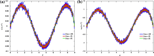Then, a set of synthetic data has been generated using the following parameters: $L=9$, $T=1$ and $N_x=N_t=1801$, where $N_x$ and $N_t$ are space and time grid sizes, respectively. The method has been implemented in Matlab and applied in noise-free and noisy cases. In the noise-corrupted case, 1, 3, 5 and 10% white Gaussian random noises with zero means have been added to the data where the noise level is evaluated using $\frac{\Vert u_{exact}-u_{approximate}{\Vert }_2}{\Vert u_{exact}{\Vert }_2}\times 100$; see Figure 1. The trapezoidal numerical integration method has been used to approximate the integrals.

Figure 1. Green solid lines represent the exact measurements, in IP1 example, while the red and blue lines represent the noisy measurements with 5 and 10% of noise, respectively. The sub-figure (a) is for the displacement $u(x,t^{\ast })$ while (b) for the acceleration $u_{tt}(x,t^{\ast })$, both at fixed time $t^{\ast }$.

Regarding the choice of the modulating functions, as mentioned before there are many functions that satisfy (3(3) $$\begin{array}{c}\hfill \left\{\begin{array}{cc}\mathit{\varphi }(x)\in C^l([0,L])\hfill & \text{(a)}\hfill \\ \text{and}\hfill & \\ {\mathit{\varphi }}^{(p)}(0)={\mathit{\varphi }}^{(p)}(L)=0,forp=0,1,2,\dots ,l-1,\hfill & \text{(b)}\hfill \end{array}\right.\end{array}$$(3) ), see e.g. 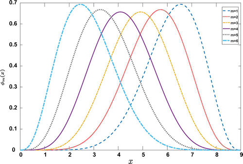[23–27,31]. In this paper, normalized polynomial-type modulating functions have been used for their simplicity. They have the following form:(45) $$\begin{array}{cc}\hfill {\mathit{\varphi }}_m(x)& ={\displaystyle \frac{\overline{\mathit{\varphi }}(x)}{{\Vert \overline{\mathit{\varphi }}(x)\Vert }_{L^2}}}\text{such that}\hfill \\ \hfill {\overline{\mathit{\varphi }}}_m(x)& ={(L-x)}^{q+m}{x}^{q+M+1-m},\hfill \end{array}$$(45)

where $m=1,2,\dots ,M$, M is the number of modulating functions and $q\in {\mathbb{R}}^{+}$ is a degree of freedom which should be chosen such that ${\mathit{\varphi }}_m(x)$ is of at least second order for all m; see Figure 2. Notice that ${\mathit{\varphi }}_m$ is normalized, i.e. ${\displaystyle {\int }_0^L{\mathit{\varphi }}_m^2(x)\mathrm{d}x=1}$. For the basis functions, polynomial-type has been used.

Figure 2. Six polynomial modulating functions where $M=6$ and $q=2$.

3.3.1. IP 1

The exact source has been chosen to be $f(x,t)=sin(x)t^2$ and $c=0.5$. At a fixed time, the exact source and the estimated one vs. different noise levels are presented in Figure 3, and the corresponding relative errors are shown in Table 1.

Figure 3. (a) Exact source (blue dashed) and estimated ones (colored) w.r.t different noise levels: 0, 1, 3, 5 and 10% of noise, where $q=2$, $I=11$ and $M=115$. (b) Estimation errors for the results in (a).

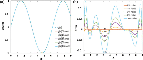
Table 1. Relative errors of $\widehat{f}(x,t^{\ast })$ vs. different noise levels.

Noise level (%)	Relative error (%)
0	0.0728
1	0.0926
3	0.2756
5	0.4593
10	0.9191

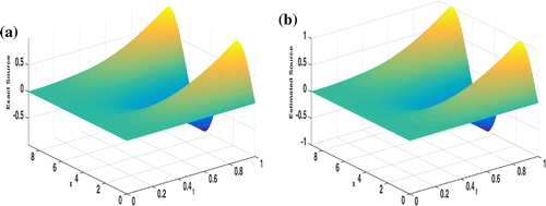
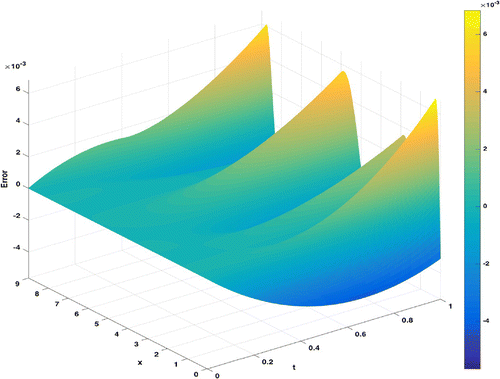
Figure 4 exhibits the exact source and the estimated one at three different times $t_1^{\ast }$, $t_2^{\ast }$ and $t_3^{\ast }$. These results, which are obtained at only three time instants, are interpolated to estimate the source f(x, t) as shown in Figures 5 and 6. For the interpolation, there are different methods that can be used to interpolate (estimate) new data points from known ones, see, for example, [32]. Here, polynomial interpolation method has been used for illustration. The relative errors for estimating f(x, t) against different noise levels are presented in Table 2. As we can see, even with 10% of noise, the estimation error is acceptable.

Figure 4. Exact source (blue dashed) and estimated one (red solid) at three fixed times. $\text{Noise level}=5\%,q=2$ and $M=115$.

Figure 5. (a) Exact source $f(x,t)=sin(x)t^2$; (b) Estimated source after interpolating the data in Figure 4. $\text{Noise level}=5\%,q=2$ and $M=115$.

Figure 6. Space–time-dependent source estimation error, $f(x,t)-\widehat{f}(x,t)$, for the result in Figure 5.

Table 2. Relative errors of $\widehat{f}(x,t)$ vs. different noise levels.

Noise level (%)	Relative error (%)
0	0.0164
1	0.0908
3	0.2670
5	0.4441
10	0.8871

3.3.1.1. IP 1 with measurements interpolation

In this part, we assume the availability of the measurements at only few points; i.e., we have $u(x_i,t^{\ast })$ and $u_{tt}(x_i,t^{\ast })$ at some points $x_i$, $i=1,2,\dots ,{\overline{N}}_x$. In this case, we first interpolate the available measurements in order to approximate them over the whole space domain [0,L]; and then we applied the MFB method to estimate the unknown $f(x,t^{\ast })$. The relative errors corresponding to different noise levels are shown in Table 3, where ${\overline{N}}_x=31$ points (${\overline{N}}_x=1.7\%N_x$) and spline interpolation have been used.

Table 3. Relative errors of $\widehat{f}(x,t^{\ast })$ vs. different noise levels when only 1.7% of the measurements are used (measurements interpolation).

Noise level (%)	Relative error (%)
0	0.1694
1	0.1837
3	0.3077
5	0.4725
10	0.9169

3.3.2. IP 2:

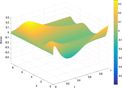
Three cases have been tested: constant velocity, space-varying velocity and space–time-dependent velocity. The exact values of the velocity in the three cases are chosen as follows: $c=5$, $c(x)=cos(x)+\frac{3}{2}$ and $c(x,t)=(cos(x)+\frac{3}{2})\sqrt{t}$, respectively. Table 4 shows the estimated values and the relative errors of the constant velocity coefficient with respect to different noise levels. The results of estimating c(x) are presented in Figure 7 and Table 5. Figures 8–9 and Table 6 show the results of estimating the space–time-dependent velocity c(x, t) after estimating and then interpolating the velocity at six time instances $t^{\ast }$.

Table 4. The estimated results for constant velocity coefficient with respect to different noise levels where the exact is $c=5$.

Noise level (%)	Estimated value	Relative error (%)
0	4.999988320728492	0.00023359
1	4.994924715399806	0.10151
3	4.984803469434329	0.30393
5	4.974690168587637	0.5062
10	4.949441615031557	1.0112

Figure 7. (a) Exact space-dependent velocity c(x) (blue dashed) and estimated ones $\widehat{c}(x)$ (colored solid) corresponding to different noise levels. (b) Estimation errors for the results in (a).

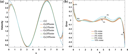
Table 5. Relative errors of $\widehat{c}(x)$ vs. different noise levels.

Noise level (%)	Relative error (%)
0	4.7014
1	4.6186
3	4.7089
5	4.9868
10	5.9880

Figure 8. Exact velocity c(x, t) (left) and estimated one $\widehat{c}(x,t)$ (right) after applying the MFB algorithm and doing interpolation; $\text{noise level}=5\%$.

Figure 9. Space–time-dependent velocity estimation error, $c(x,t)-\widehat{c}(x,t)$, for the result in Figure 8.

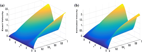
Table 6. Relative errors of $\widehat{c}(x,t)$ vs. different noise levels.

Noise level (%)	Relative error (%)
0	6.5658
1	6.6397
3	7.2652
5	8.4162
10	12.2628

3.3.3. IP3:

For joint estimation, we set $f(x)=c(x)=sin(x)+1$. The estimated source and velocity in this joint estimation are shown in Figures 10 and 11, respectively. The corresponding relative errors are presented in Table 7.

Figure 10. (a) Exact source f(x) (blue dashed) and estimated ones in the joint estimation $\widehat{f}(x,t^{\ast })$ (coloured solid) corresponding to different noise levels. (b) Estimation errors for the results in (a).

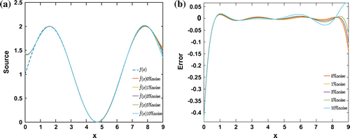
Figure 11. (a) Exact velocity c(x) (blue dashed) and the estimated ones in the joint estimation $\widehat{c}(x)$ (coloured solid) corresponding to different noise levels. (b) Estimation errors for the results in (a).

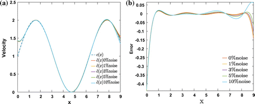
Table 7. Relative errors of estimating f(x) and c(x) in the joint estimation vs. different noise levels.

Noise level (%)	Relative error (%)
0	3.9745
1	4.0151
3	4.0492
5	4.0466
10	4.1122

The presented figures and tables show that the estimated unknown is in quite good agreement with the exact one; therefore, the MFB method is an efficient and a robust method for solving parameters and source estimation for linear PDE. The method can be easily extended to identify parameters of non-linear PDE as shown in the next section.

4. Parameter estimation for the fifth-order KdV equation

4.1. Method

The fifth-order non-linear KdV equation has the following form:(46) $$\begin{array}{c}\hfill u_t(x,t)+{\mathit{\alpha }}_{1}u(x,t)u_x(x,t)+{\mathit{\alpha }}_2{u}_{xxx}(x,t)-{\mathit{\alpha }}_3{u}_{(}x,t)=0,\end{array}$$(46)

where ${\mathit{\alpha }}_1$, ${\mathit{\alpha }}_2$ and ${\mathit{\alpha }}_3$ are positive parameters. This equation is used to model different phenomena such as capillary–gravity water waves, chains of coupled oscillators and magneto-acoustic waves in plasma.[33–35] The parameters, ${\mathit{\alpha }}_1$, ${\mathit{\alpha }}_2$ and ${\mathit{\alpha }}_3$, are related to properties of the physical medium under consideration. Thus, estimating these parameters can be used to validate the applicability of this equation for particular media.[36] Hence, the following inverse problem can be defined:

Given $u(x,t^{\ast })$ and $u_t(x,t^{\ast })$ at a fixed time $t^{\ast }$, find ${\mathit{\alpha }}_1$, ${\mathit{\alpha }}_2$ and ${\mathit{\alpha }}_3$.

The following corollary gives a solution to this inverse problem using the MFB method.

Corollary 3:

Let ${\mathit{\alpha }}_1$, ${\mathit{\alpha }}_2$ and ${\mathit{\alpha }}_3$ be unknown parameters in (46(48) $$\begin{array}{cc}\hfill {\mathcal{A}}_m& ={\left[\begin{array}{c}{\displaystyle -\frac{1}{2}{\int }_0^L{u}^2(x,t^{\ast }){\mathit{\varphi }}_m^{{}^{\prime }}(x)\mathrm{d}x}\\ {\displaystyle -{\int }_0^{L}u(x,t^{\ast }){\mathit{\varphi }}_m^{{}^{″\prime }}(x)\mathrm{d}x}\\ {\displaystyle {\int }_0^{L}u(x,t^{\ast }){\mathit{\varphi }}_m^{{}^{″″\prime }}(x)\mathrm{d}x}\end{array}\right]}^{tr},\hfill \end{array}$$(48) ), and let ${\{{\mathit{\varphi }}_m(x)\}}_{m=1}^{m=M}$ be a class of at least fifth-order modulating functions with $M\ge 3$. Then, the unknown parameters can be estimated by solving the following linear system:(47) $$\begin{array}{c}\hfill \mathcal{A}\left\}\right\}\mathrm{\Gamma }=K,\end{array}$$(47)

where the rows of the $M\times 3$ matrix $\mathcal{A}$, the elements of the vector K and the vector $\mathrm{\Gamma }$ are(48) $$\begin{array}{cc}\hfill {\mathcal{A}}_m& ={\left[\begin{array}{c}{\displaystyle -\frac{1}{2}{\int }_0^L{u}^2(x,t^{\ast }){\mathit{\varphi }}_m^{{}^{\prime }}(x)\mathrm{d}x}\\ {\displaystyle -{\int }_0^{L}u(x,t^{\ast }){\mathit{\varphi }}_m^{{}^{″\prime }}(x)\mathrm{d}x}\\ {\displaystyle {\int }_0^{L}u(x,t^{\ast }){\mathit{\varphi }}_m^{{}^{″″\prime }}(x)\mathrm{d}x}\end{array}\right]}^{tr},\hfill \end{array}$$(48) (49) $$\begin{array}{cc}\hfill K_m& =-{\int }_0^L{u}_t(x,t^{\ast }){\mathit{\varphi }}_m(x)\mathrm{d}x,\hfill \end{array}$$(49)

and(50) $$\begin{array}{c}\hfill \mathrm{\Gamma }={\left[\begin{array}{ccc}{\mathit{\alpha }}_1& {\mathit{\alpha }}_2& {\mathit{\alpha }}_3\end{array}\right]}^{tr},\end{array}$$(50)

respectively.

Appendix 3 provides details of the proof.

4.2. Numerical simulations

For numerical simulations, let ${\mathit{\alpha }}_1={\mathit{\alpha }}_2={\mathit{\alpha }}_3=1$; then, (46(48) $$\begin{array}{cc}\hfill {\mathcal{A}}_m& ={\left[\begin{array}{c}{\displaystyle -\frac{1}{2}{\int }_0^L{u}^2(x,t^{\ast }){\mathit{\varphi }}_m^{{}^{\prime }}(x)\mathrm{d}x}\\ {\displaystyle -{\int }_0^{L}u(x,t^{\ast }){\mathit{\varphi }}_m^{{}^{″\prime }}(x)\mathrm{d}x}\\ {\displaystyle {\int }_0^{L}u(x,t^{\ast }){\mathit{\varphi }}_m^{{}^{″″\prime }}(x)\mathrm{d}x}\end{array}\right]}^{tr},\hfill \end{array}$$(48) ) is a Kawahara equation. Kawahara equation with an initial condition $u(x,0)=\frac{105}{169}{\text{sech}}^4\left[\frac{1}{2\sqrt{1}3}x\right]$ has the following exact solution [37]:(51) $$\begin{array}{c}\hfill u(x,t)=\frac{105}{169}{\text{sech}}^4\left[\frac{1}{2\sqrt{1}3}\left(x-\frac{36t}{169}\right)\right].\end{array}$$(51)

Figure 12 and Table 8 exhibit the estimated parameters values and the relative errors, respectively, where $L=60$, $T=50$, $N_x=N_t=601$ and the degree of freedom q in (45(47) $$\begin{array}{c}\hfill \mathcal{A}\left\}\right\}\mathrm{\Gamma }=K,\end{array}$$(47) ) is chosen such that ${\mathit{\varphi }}_m(x)$ is at least of order five. These results show that the identification of the parameters is successful in both noise-free and noisy cases.

Figure 12. Blue, red and green bars represent the estimated values of the parameters ${\mathit{\alpha }}_1,{\mathit{\alpha }}_2$ and ${\mathit{\alpha }}_3$ in Kawarah equation, respectively. The exact values are ${\mathit{\alpha }}_1={\mathit{\alpha }}_2={\mathit{\alpha }}_3=1$ and the estimation is done w.r.t different noise levels; $q=9$ and $M=27$.

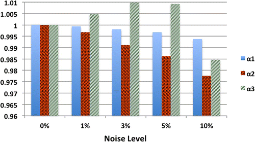
Table 8. The relative errors of estimating the parameters ${\mathit{\alpha }}_1,{\mathit{\alpha }}_2$ and ${\mathit{\alpha }}_3$ in Kawahara equation w.r.t different noise levels.

Noise level (%)	${\displaystyle \frac{|{\mathit{\alpha }}_1-{\widehat{\mathit{\alpha }}}_1|}{|{\mathit{\alpha }}_1|}}\times 100$	${\displaystyle \frac{|{\mathit{\alpha }}_2-{\widehat{\mathit{\alpha }}}_2|}{|{\mathit{\alpha }}_2|}}\times 100$	${\displaystyle \frac{|{\mathit{\alpha }}_3-{\widehat{\mathit{\alpha }}}_3|}{|{\mathit{\alpha }}_3|}}\times 100$
0	1.8208e$-$11	1.4352e$-$10	1.2131e$-$09
1	0.066152	0.31912	0.47765
3	0.19532	0.89011	0.99108
5	0.32077	1.3756	0.93457
10	0.6219	2.2509	1.5333

For constant unknowns, as in this example, it can be enough to have the measurements at a suitable sub-domain $\mathit{\omega }=[0,L^{\ast }]\subset [0,L]$. Estimating the three parameters in Kawahara equation with different values for $L^{\ast }$, $L^{\ast }\le L$, is shown in Figure 13. From this figure, we observe that in the noise-free case, the error is small even when the data are available only in the first-third of the whole interval. In the noisy case, this sub-domain should be increased to have an acceptable estimation error. In both cases, the error generally decreases as $L^{\ast }$ increases.

Figure 13. Relative errors (in %) for estimating ${\mathit{\alpha }}_1,{\mathit{\alpha }}_2$ and ${\mathit{\alpha }}_3$ simultaneously in Kawahara equation w.r.t different $L^{\ast }$. (a) in noise-free case and (b) with 5% of noise on the measurements.

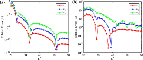
Figure 14. Number of modulating functions vs. the relative errors for (a) IP1, (b) IP2, (c) IP3 source estimation and (d) IP3 velocity estimation. In these figures, 5% of the noise was added to the measurements.

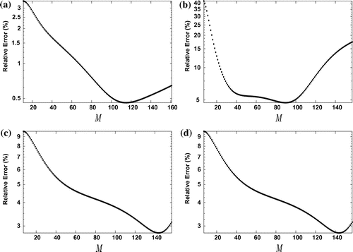
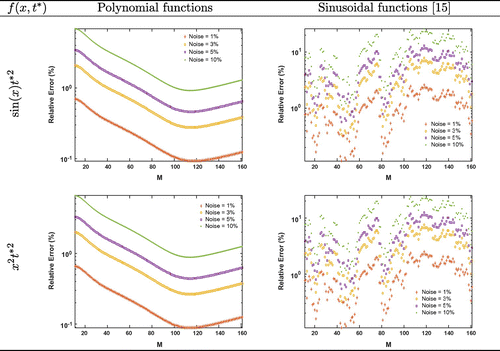
Figure 15. Number of modulating functions vs. the relative error in IP1 w.r.t different noise levels and unknown source. Two types of modulating functions have been applied: polynomial modulating functions and sinusoidal modulating functions.

Similar to the procedure developed for the wave equation example, one can estimate space-dependent coefficients in the fifth-order KdV equation. In addition, the MFB method can be applied to estimate parameters in other high-order non-linear PDEs such as the sixth-order Boussinesq equation and take advantage of the properties of modulating functions to transfer the spatial derivatives to the modulating functions which can be computed analytically.

5. Discussion

The numerical part in this paper confirms the efficiency of the modulating functions-based method and its simple implementation. In addition, the obtained results have shown the good performance of this method and its success even with high levels of noise.

The number of modulating functions, M, plays an important role in the performance of the method; (see Figure 14). Figure 14 exhibits the number of modulating functions vs. the relative error for IP1, IP2 and IP3. Interestingly, it shows that the accuracy of the estimation can be improved by increasing M, especially in the noisy case. In addition, it shows that there exists a unique optimal number of modulating functions, $M^{\ast }$, in the studied examples. However, the estimation is generally good for a relatively large interval for M. Also, it proves that this optimal number depends on the considered problem. From this observation, it is worthy to know under a specific parameter identification problem and after choosing the type of modulating functions how the relative error, as a function of M, is affected by the noise level and the nature of the unknown functions. Figure 15 illustrates this behaviour in the noisy case in unknown input case. In this case, the relative error, with respect to the number of modulating functions, is invariant with respect to the noise level and the type of the unknown. This latter result offers a way to select an optimal number of modulating functions for real applications. In other words, one can set a synthetic function for the unknown input, apply the method and compute the error for different numbers of modulating functions to find the optimal one, $M^{\ast }$, and finally this $M^{\ast }$ might be a good guess for the real inverse problem. This result is expected for the unknown input problem (IP1) because the matrix $\mathcal{A}$ is independent of the unknown and the measurements (see Equation (23a(25a) $$\begin{array}{c}\hfill \mathbf{IP}\mathbf{3}:\left\{\begin{array}{c}\mathcal{A}=[A_1{A}_2\dots A_{\overline{n}}-A_f],\text{such that the elements}\hfill \\ A_{s_{mi}},s=1,\dots ,\overline{n},\text{and}{\overline{A}}_{f_{mj}}\text{are as in}\text{(24a) and}\text{(23a), respectively;}\hfill \\ {\displaystyle K_m=-{\int }_0^L\mathbb{T}u(x,t^{\ast }){\mathit{\varphi }}_m(x)\mathrm{d}x;}\hfill \\ i=1,2,\dots ,I_s;j=1,2,\dots ,I_0;m=1,2,\dots ,M;\text{and}M\ge {\sum }_{\overline{s}=0}^{\overline{n}}{I}_{\overline{s}}.\hfill \end{array}\right.\end{array}$$(25a) )).

The choice of an appropriate number of basis functions used to expand the space-varying unknown functions is also important. Choosing this number may lead to ill-conditioning issues. Moreover, if this number is significantly smaller than the appropriate one, we lose accuracy. Hence, this number must be selected such that the numerical stability and accuracy are relatively good.

The MFB method can be also applied to the case of measurements that are available at fixed points in the space instead of fixed time instants. However, time-dependent modulating functions, $\mathit{\varphi }(t)$, must be used in this case.

In a forthcoming study, we will consider the case of reduced number of measurements and study the solution of the inverse problems with the MFB method. An example of this study includes solving the previous inverse problems using field measurements $u(x,t^{\ast })$ only (without $\mathbb{T}u(x,t^{\ast })$).

6. Conclusion

In this paper, the MFB method for solving inverse problems for 1D-PDEs has been proposed. The well-posedness of the MFB solution has been studied. As illustrative examples, the method has been applied on the wave equation (linear 1D-PDE) and on the fifth-order KdV (non-linear 1D-PDE) to estimate different unknowns. By applying the MFB method, the problem has been converted to a system of algebraic equations which is linear in the unknowns. Then, these unknowns have been estimated using least square algorithms. Numerical simulations in both noise-free and noise-corrupted cases have shown good performance and robustness of this method. The noise error contribution has been also studied and an upper bound for it has been derived.

Future study will investigate the choice of the number of basis in order to propose an efficient and systematic method for selecting this number. In addition, we will extend the MFB method to the estimation of discontinuous space–time-dependent unknowns, which are more realistic for real applications.

Acknowledgements

The authors would like to thank the anonymous reviewers for their valuable comments and suggestions that have led to an improved version of this paper.

Additional information

Funding

Research reported in this publication was supported by King Abdullah University of Science and Technology (KAUST).

Notes

No potential conflict of interest was reported by the authors.

Appendix 1

Proof of Corollary (1)

IP1

First, at fixed time $t^{\ast }$, the PDE in (26(28a) $$\begin{array}{cc}\hfill \text{IP1:}& {\displaystyle {\mathcal{A}}_{mi}={\int }_0^L{\mathit{\varphi }}_m(x){\mathit{\xi }}_i(x)\mathrm{d}x,}\hfill \end{array}$$(28a) ) is multiplied by ${\mathit{\varphi }}_m(x)$ and integrated over [0, L]:(A1) $$\begin{array}{c}\hfill {\int }_0^L{\mathit{\varphi }}_m(x)u_{tt}(x,t^{\ast })\mathrm{d}x-{\int }_0^L{\mathit{\varphi }}_m(x)c(x,t^{\ast })u_{xx}(x,t^{\ast })\mathrm{d}x={\int }_0^L{\mathit{\varphi }}_m(x)f(x,t^{\ast })\mathrm{d}x.\end{array}$$(A1)

Then, we apply integration by parts twice to the second integral in (A1(A1) $$\begin{array}{c}\hfill {\int }_0^L{\mathit{\varphi }}_m(x)u_{tt}(x,t^{\ast })\mathrm{d}x-{\int }_0^L{\mathit{\varphi }}_m(x)c(x,t^{\ast })u_{xx}(x,t^{\ast })\mathrm{d}x={\int }_0^L{\mathit{\varphi }}_m(x)f(x,t^{\ast })\mathrm{d}x.\end{array}$$(A1) ):(A2) $$\begin{array}{c}\hfill {\int }_0^L{\mathit{\varphi }}_m(x)u_{tt}(x,t^{\ast })\mathrm{d}x-{\int }_0^L{\left[{\mathit{\varphi }}_m(x)c(x,t^{\ast })\right]}^{″}u(x,t^{\ast })\mathrm{d}x={\int }_0^L{\mathit{\varphi }}_m(x)f(x,t^{\ast })\mathrm{d}x.\end{array}$$(A2)

Finally, by writing $f(x,t^{\ast })$ in its basis expansion, system (27(28b) $$\begin{array}{cc}\hfill \text{IP2:}& {\displaystyle {\mathcal{A}}_{mi}={\int }_0^{L}u(x,t^{\ast }){\left[{\mathit{\varphi }}_m(x){\mathit{\xi }}_i(x)\right]}^{″}\mathrm{d}x,}\hfill \end{array}$$(28b) ) is obtained with components as in (28a(28a) $$\begin{array}{cc}\hfill \text{IP1:}& {\displaystyle {\mathcal{A}}_{mi}={\int }_0^L{\mathit{\varphi }}_m(x){\mathit{\xi }}_i(x)\mathrm{d}x,}\hfill \end{array}$$(28a) ) and (29a(29a) $$\begin{array}{cc}\hfill \text{IP1:}{K}_m& {\displaystyle ={\int }_0^L{u}_{tt}(x,t^{\ast }){\mathit{\varphi }}_m(x)\mathrm{d}x-{\int }_0^{L}u(x,t^{\ast }){\left[{\mathit{\varphi }}_m(x)c(x,t^{\ast })\right]}^{″}\mathrm{d}x,}\hfill \end{array}$$(29a) ).

IP2

Equation (26(28a) $$\begin{array}{cc}\hfill \text{IP1:}& {\displaystyle {\mathcal{A}}_{mi}={\int }_0^L{\mathit{\varphi }}_m(x){\mathit{\xi }}_i(x)\mathrm{d}x,}\hfill \end{array}$$(28a) ) is first multiplied by ${\mathit{\varphi }}_m(x)$, where $c=c(x)$, and integrated over the space interval [0,L]; we obtain:(A3) $$\begin{array}{c}\hfill {\int }_0^L{\mathit{\varphi }}_m(x)u_{tt}(x,t^{\ast })\mathrm{d}x-{\int }_0^L{\mathit{\varphi }}_m(x)c(x)u_{xx}(x,t^{\ast })\mathrm{d}x={\int }_0^L{\mathit{\varphi }}_m(x)f(x)\mathrm{d}x.\end{array}$$(A3)

After that, we integrate the second term on the left-hand side by parts twice, and so$$\begin{array}{c}\hfill {\int }_0^{L}u(x,t^{\ast }){\left[c(x){\mathit{\varphi }}_m(x)\right]}^{″}\mathrm{d}x={\int }_0^L{\mathit{\varphi }}_m(x)u_{tt}(x,t^{\ast })\mathrm{d}x-{\int }_0^L{\mathit{\varphi }}_m(x)f(x)\mathrm{d}x.\end{array}$$

Then, by writting c(x) in its basis expansion, system (27(28b) $$\begin{array}{cc}\hfill \text{IP2:}& {\displaystyle {\mathcal{A}}_{mi}={\int }_0^{L}u(x,t^{\ast }){\left[{\mathit{\varphi }}_m(x){\mathit{\xi }}_i(x)\right]}^{″}\mathrm{d}x,}\hfill \end{array}$$(28b) ) is obtained with components as in (28b(28b) $$\begin{array}{cc}\hfill \text{IP2:}& {\displaystyle {\mathcal{A}}_{mi}={\int }_0^{L}u(x,t^{\ast }){\left[{\mathit{\varphi }}_m(x){\mathit{\xi }}_i(x)\right]}^{″}\mathrm{d}x,}\hfill \end{array}$$(28b) ) and (29b(29b) $$\begin{array}{cc}\hfill \text{IP2:}{K}_m& {\displaystyle ={\int }_0^L[u_{tt}(x,t^{\ast })-f(x,t^{\ast })]{\mathit{\varphi }}_m(x)\mathrm{d}x,}\hfill \end{array}$$(29b) ).

Appendix 2

Proof of Corollary (2)

System (33(35) $$\begin{array}{c}\hfill {\mathrm{{\rm Y}}}_{mj}={\int }_0^{L}u(x,t^{\ast }){\left[{\mathit{\upsilon }}_j(x){\mathit{\varphi }}_m(x)\right]}^{″}\mathrm{d}x,\end{array}$$(35) ) can be obtained by doing the same steps in A.2: Equation (26(28a) $$\begin{array}{cc}\hfill \text{IP1:}& {\displaystyle {\mathcal{A}}_{mi}={\int }_0^L{\mathit{\varphi }}_m(x){\mathit{\xi }}_i(x)\mathrm{d}x,}\hfill \end{array}$$(28a) ) is first multiplied by ${\mathit{\varphi }}_m(x)$; integrated over the interval [0,L]; then, integration by parts is applied to the second integral, and finally, the unknowns are written in their basis expansion, $f_I(x)={\sum }_{i=0}^I{\mathit{\gamma }}_i{\mathit{\xi }}_i(x)$ and $c_J(x)={\sum }_{j=0}^J{\mathit{\beta }}_j{\mathit{\upsilon }}_j(x)$.

Appendix 3

Proof of Corollary (3)

STEP 1: Fix the time in Equation (46(48) $$\begin{array}{cc}\hfill {\mathcal{A}}_m& ={\left[\begin{array}{c}{\displaystyle -\frac{1}{2}{\int }_0^L{u}^2(x,t^{\ast }){\mathit{\varphi }}_m^{{}^{\prime }}(x)\mathrm{d}x}\\ {\displaystyle -{\int }_0^{L}u(x,t^{\ast }){\mathit{\varphi }}_m^{{}^{″\prime }}(x)\mathrm{d}x}\\ {\displaystyle {\int }_0^{L}u(x,t^{\ast }){\mathit{\varphi }}_m^{{}^{″″\prime }}(x)\mathrm{d}x}\end{array}\right]}^{tr},\hfill \end{array}$$(48) ) at $t^{\ast }$, and then multiply the equation by the modulating functions ${\mathit{\varphi }}_m(x)$:(C1) $$\begin{array}{cc}& u_t(x,t^{\ast }){\mathit{\varphi }}_m(x)+{\mathit{\alpha }}_{1}u(x,t^{\ast })u_x(x,t^{\ast }){\mathit{\varphi }}_m(x)\hfill \\ \hfill & +{\mathit{\alpha }}_2{u}_{xxx}(x,t^{\ast }){\mathit{\varphi }}_m(x)-{\mathit{\alpha }}_3{u}_{(}x,t^{\ast }){\mathit{\varphi }}_m(x)=0.\hfill \end{array}$$(C1)

STEP 2: Integrate over the space interval:(C2) $$\begin{array}{cc}& {\int }_0^L{u}_t(x,t^{\ast }){\mathit{\varphi }}_m(x)\mathrm{d}x+{\mathit{\alpha }}_1{\int }_0^{L}u(x,t^{\ast })u_x(x,t^{\ast }){\mathit{\varphi }}_m(x)\mathrm{d}x\hfill \\ \hfill & +{\mathit{\alpha }}_2{\int }_0^L{u}_{xxx}(x,t^{\ast }){\mathit{\varphi }}_m(x)\mathrm{d}x-{\mathit{\alpha }}_3{\int }_0^L{u}_{(}x,t^{\ast }){\mathit{\varphi }}_m(x)\mathrm{d}x=0.\hfill \end{array}$$(C2)

STEP 3: By applying the integration by parts formula, once to the second integral, three times to the third integral and five times to the fourth integral in (C2(C2) $$\begin{array}{cc}& {\int }_0^L{u}_t(x,t^{\ast }){\mathit{\varphi }}_m(x)\mathrm{d}x+{\mathit{\alpha }}_1{\int }_0^{L}u(x,t^{\ast })u_x(x,t^{\ast }){\mathit{\varphi }}_m(x)\mathrm{d}x\hfill \\ \hfill & +{\mathit{\alpha }}_2{\int }_0^L{u}_{xxx}(x,t^{\ast }){\mathit{\varphi }}_m(x)\mathrm{d}x-{\mathit{\alpha }}_3{\int }_0^L{u}_{(}x,t^{\ast }){\mathit{\varphi }}_m(x)\mathrm{d}x=0.\hfill \end{array}$$(C2) ), one can obtain:(C3) $$\begin{array}{cc}& {\int }_0^L{u}_t(x,t^{\ast }){\mathit{\varphi }}_m(x)\mathrm{d}x-\frac{1}{2}{\int }_0^L{\mathit{\alpha }}_1{u}^2(x,t^{\ast }){\mathit{\varphi }}_m^{\prime }(x)\mathrm{d}x\hfill \\ \hfill & -{\int }_0^L{\mathit{\alpha }}_{2}u(x,t^{\ast }){\mathit{\varphi }}_m^{″\prime }(x)\mathrm{d}x+{\int }_0^L{\mathit{\alpha }}_{3}u(x,t^{\ast }){\mathit{\varphi }}_m^{″″\prime }(x)\mathrm{d}x=0.\hfill \end{array}$$(C3)

The first integral in (C3(C3) $$\begin{array}{cc}& {\int }_0^L{u}_t(x,t^{\ast }){\mathit{\varphi }}_m(x)\mathrm{d}x-\frac{1}{2}{\int }_0^L{\mathit{\alpha }}_1{u}^2(x,t^{\ast }){\mathit{\varphi }}_m^{\prime }(x)\mathrm{d}x\hfill \\ \hfill & -{\int }_0^L{\mathit{\alpha }}_{2}u(x,t^{\ast }){\mathit{\varphi }}_m^{″\prime }(x)\mathrm{d}x+{\int }_0^L{\mathit{\alpha }}_{3}u(x,t^{\ast }){\mathit{\varphi }}_m^{″″\prime }(x)\mathrm{d}x=0.\hfill \end{array}$$(C3) ) represents the mth row of K as in (49(51) $$\begin{array}{c}\hfill u(x,t)=\frac{105}{169}{\text{sech}}^4\left[\frac{1}{2\sqrt{1}3}\left(x-\frac{36t}{169}\right)\right].\end{array}$$(51) ) while the second, third and fourth integrals form the mth row of $\mathcal{A}$ multiplied by the vector of unknowns $\mathrm{\Gamma }$, see (48(50) $$\begin{array}{c}\hfill \mathrm{\Gamma }={\left[\begin{array}{ccc}{\mathit{\alpha }}_1& {\mathit{\alpha }}_2& {\mathit{\alpha }}_3\end{array}\right]}^{tr},\end{array}$$(50) ) and (50(50) $$\begin{array}{c}\hfill \mathrm{\Gamma }={\left[\begin{array}{ccc}{\mathit{\alpha }}_1& {\mathit{\alpha }}_2& {\mathit{\alpha }}_3\end{array}\right]}^{tr},\end{array}$$(50) ).

References

- Robinson EA. Predictive decomposition of time series with application to seismic exploration. Geophysics. 1967;32:418–484.
- Cameron M, Fomel S, Sethian J. Inverse problem in seismic imaging. PAMM. 2007;7:1024803–1024804.
- Fear E, Stuchly M. Microwave detection of breast cancer. IEEE Trans. Microwave Theory Tech. 2000;48:1854–1863.
- Kirsch A. Characterization of the shape of a scattering obstacle using the spectral data of the far field operator. Inverse Prob. 1998;14:1489–1512.
- Muniz W, Ramos F, de Campos Velho H. Entropy-and tikhonov-based regularization techniques applied to the backwards heat equation. Comput. Math. Appl. 2000;40:1071–1084.
- Clason C, Klibanov MV. The quasi-reversibility method for thermoacoustic tomography in a heterogeneous medium. SIAM J. Sci. Comput. 2007;30:1–23.
- Han H, Ling L, Takeuchi T. An energy regularization for cauchy problems of laplace equation in annulus domain. Commun. Comput. Phys. 2011;9:878–896.
- Poli L, Oliveri G, Rocca P, et al. Bayesian compressive sensing approaches for the reconstruction of two-dimensional sparse scatterers under te illuminations. IEEE Trans. Geosci. Remote Sens. 2013;51:2920–2936.
- Moireau P, Chapelle D, Le Tallec P. Joint state and parameter estimation for distributed mechanical systems. Comput. Methods Appl. Mech. Eng. 2008;197:659–677.
- Ramdani K, Tucsnak M, Weiss G. Recovering the initial state of an infinite-dimensional system using observers. Automatica. 2010;46:1616–1625.
- Asiri S, Laleg-Kirati T, Zayane C. Inverse source problem for a one-dimensional wave equation using observers. In: 11th International Conference on Mathematical and Numerical Aspects of Waves; Tunisia; 2013. p. 149–150.
- Tucsnak M, Weiss G. From exact observability to identification of singular sources. Math. Control Signals Syst. 2014;27:1–21.
- Zuazua E. Propagation, observation, control and numerical approximation of waves. SIAM Rev. 2005;47:197–243.
- Shinbrot M. On the analysis of linear and nonlinear dynamical systems from transient-response data. National Advisory Committee for Aeronautics NACA; 1954.
- Shinbrot M. On the analysis of linear and nonlinear systems. Trans. ASME. 1957;79:547–552.
- Perdreauville FJ, Goodson R. Identification of systems described by partial differential equations. J. Fluids Eng. 1966;88:463–468.
- Fairman F, Shen D. Parameter identification for a class of distributed systems. Int. J. Control. 1970;11:929–940.
- Co TB, Ungarala S. Batch scheme recursive parameter estimation of continuous-time systems using the modulating functions method. Automatica. 1997;33:1185–1191.
- Liu DY, Laleg-Kirati TM, Perruquetti W, et al. Non-asymptotic state estimation for a class of linear time-varying systems with unknown inputs. IFAC P. Vol. 2014;47:3732–3738.
- Liu DY, Laleg-Kirati TM. Robust fractional order differentiators using generalized modulating functions method. Signal Process. 2015;107:395–406.
- Liu DY, Tian Y, Boutat D, et al. An algebraic fractional order differentiator for a class of signals satisfying a linear differential equation. Signal Process. 2015;116:78–90.
- Aldoghaither A, Liu D, Laleg-Kirati T. A novel approach for parameter and differentiation order estimation for a space fractional advection dispersion equation. SIAM J. Sci. Comput. 2015;37:A2813–A2839.
- Takaya K. The use of hermite functions for system identification. IEEE Trans. Autom. Control. 1968;13:446–447.
- Preisig H, Rippin D. Theory and application of the modulating function method–i. review and theory of the method and theory of the spline-type modulating functions. Comput. Chem. Eng. 1993;17:1–16.
- Saha DC, Rao BP, Rao GP. Structure and parameter identification in linear continuous lumped systems: the poisson moment functional approach. Int. J. Control. 1982;36:477–491.
- Patra A, Unbehauen H. Identification of a class of nonlinear continuous-time systems using hartley modulating functions. Int. J. Control. 1995;62:1431–1451.
- Pearson A, Lee F. Parameter identification of linear differential systems via fourier based modulating functions. Control-Theory Adv. Technol. 1985;1:239–266.
- Fliess M. Analyse non standard du bruit. C.R. Math. 2006;342:797–802.
- Fliess M. Critique du rapport signal à bruit en communications numériques-questioning the signal to noise ratio in digital communications. ARIMA (Revue africaine d’informatique et de Mathématiques appliquées). 2008;9:419–429.
- Liberzon D. Calculus of variations and optimal control theory: a concise introduction. New Jersey: Princeton University Press; 2012.
- Liu DY, Laleg-Kirati TM, Gibaru O, et al. Identification of fractional order systems using modulating functions method. In: American Control Conference (ACC), 2013. IEEE, Washington, DC; 2013. p. 1679–1684.
- Rabiner LR. Multirate digital signal processing. New Jersey: Prentice Hall PTR; 1996.
- Benney D. General theory for interactions between short and long waves. Stud. Appl. Math. 1977;56:81–94. cited By 110.
- Gorshkov K, Ostrovsky L. Interactions of solitons in nonintegrable systems: direct perturbation method and applications. Phys. D: Nonlinear Phenom. 1981;3:428–438.
- Bridges T, Derks G. Linear instability of solitary wave solutions of the kawahara equation and its generalizations. SIAM J. Math. Anal. 2002;33:1356–1378.
- Janno J, Šeletski A. Reconstruction of coefficients of higher order nonlinear wave equations by measuring solitary waves. Wave Motion. 2014;52:15–25.
- Kaya D. An explicit and numerical solutions of some fifth-order kdv equation by decomposition method. Appl. Math. Comput. 2003;144:353–363.