Detection-Identification of multiple unknown time-dependent point sources in a 2D transport equation: application to accidental pollution

Abstract

We address the nonlinear inverse source problem of identifying multiple unknown time-dependent point sources occurring in a two-dimensional evolution advection–dispersion–reaction equation. Provided to be available within the monitored domain interfaces for recording the generated state and its flux crossing each suspected zone where a source could occur, we establish a constructive identifiability theorem based on an introduced dispersion-current function that yields uniqueness of the unknown elements defining all occurring sources. Then, the established theorem leads to develop a detection-identification method that goes throughout the monitored domain to detect in each suspected zone whether there exists or not an occurring source. Once a source is detected, the developed method determines lower and upper bounds of the mean value discharged by its unknown time-dependent intensity function. Thereafter, the method localizes the sought position of the detected source as the unique solution of an equation satisfied by the introduced dispersion-current function and identifies its unknown intensity function from solving an associated deconvolution problem. Ultimately, the unknown number of occurring sources is deduced as the sum of all detected-identified active sources. Some numerical experiments on a variant of the surface water BOD pollution model are presented.

Keywords:

• Non-linear inverse source problem
• data assimilation
• optimization and control technique
• advection–dispersion–reaction equation
• surface water pollution

1. Introduction

Non-linear inverse source problems are usually known to be somewhat delicate since in general there is no identifiability (uniqueness) of unknown sources under an abstract form using only local boundary or/and internal measurements related to the associated state, see [1] for a counterexample. In the literature, to overcome this difficulty authors generally assume to be available some a priori information on the form of the sought source: for example, time-independent sources are treated by Cannon [2] using spectral theory, then by Engl et al. [3] using the approximated controllability of the heat equation. The results of this last paper are generalized by Yamamoto in [4] to sources of separated time and space variables where the time-dependent part is assumed to be known and null at the initial time, then recently in [5] to sources where the known time-dependent part of the sought source could also depend on the space variables and the involved differential operator is a time fractional parabolic equation. Hettlich and Rundell addressed in [6] the two-dimensional (2D) inverse source problem for the heat equation with as a source the characteristic function associated to a subset of a disk. El Badia and Hamdi treated in [7,8] the case of a time-dependent point source occurring in a one-dimensional (1D) evolution transport equation with constant coefficients. Then, Hamdi and Mahfoudhi extended this study in [9] to the case of equations with spatially varying coefficients and Ben Belgacem et al. [10,11] to the case of a moving time-dependent point source. A detection-identification method for multiple unknown time-dependent point sources in a one-dimensional evolution transport equation was recently developed by Hamdi in [12]. Hamdi and Mahfoudhi treated in [13] the identification of a single time-dependent point source in a two-dimensional evolution advection–dispersion–reaction equation. El Badia et al. studied in [14] the case of multiple time-dependent moving point sources in a two-dimensional evolution advection–diffusion–reaction equation.

The present study is motivated by the results established in the two recent papers.[12,14] Firstly, in [14] authors reported some difficulties encountered by the proposed identification procedure that consists of minimizing the two objective functions least squares and Kohn–Vogelius. In fact, the identifiability result in [14] is based on the unique continuation Theorem that suggests to identify the unknown elements defining whatever finite number of time-dependent point sources using only local boundary measurements taken at any non-empty part of the boundary. In our view, that is an ideal theoretical framework which doesn’t give any visibility on how to proceed in terms of identification and in practice doesn’t take into account the flow properties: for example, the case of an advection dominant flow would imply that using only data reaching back the inflow boundary doesn’t enable to cover the entire activity of downstream occurring sources as well as the case of a flow defined by a velocity field fulfilling the no mass penetrate a solid interface and no-slip conditions along the lateral boundaries which leads to a similar conclusion for using only data reaching these boundaries. Moreover, in terms of identification although in [14] the authors employed measurements taken on the whole boundary of the considered domain, the least squares approach doesn’t enable to identify more than one active source whereas the Kohn–Vogelius approach identifies two sources only under some particular conditions: sources should be well separated and diffusion coefficient should be very small to avoid rapid intermixing. Secondly, the recent results established in [12] prove that in the case of a one-dimensional advection–diffusion–reaction equation, local measurements taken only upstream and/or downstream all occurring sources don’t yield uniqueness of the unknown elements defining more than one time-dependent point source.

The originality of the present study consists in establishing a constructive identifiability theorem that leads to develop a detection-identification method able to identify accurately multiple unknown time-dependent point sources occurring in a two-dimensional evolution advection–dispersion–reaction equation from some local measurements taking into account the flow properties. A motivation for our study is a typical problem associated with environmental monitoring that aims to identify unknown pollution sources occurring in surface water. For example, in a river the involved unknown pollution sources can be identified from measuring the BOD (Biochemical Oxygen Demand) concentration which represents the amount of dissolved oxygen consumed by the micro-organisms during the oxidation process.[15,16] The paper is organized as follows: Section 2 is devoted to stating the problem, assumptions and proving some technical results for later use. In Section 3, based on an introduced dispersion-current function, we establish a constructive identifiability theorem that yields uniqueness of the unknown elements defining the occurring sources. Section 4 is reserved to develop a detection-identification method that goes throughout the monitored domain to detect the presence of all occurring active sources. Once a source is detected, the developed method determines lower and upper bounds of the mean value discharged by its unknown time-dependent intensity function, localizes its sought position and identifies its intensity function. Some numerical experiments on a variant of the surface water BOD pollution model are presented in Section5.

2. Problem statement

Let $T>0$ be a final monitoring time and $\mathrm{\Omega }$ be a bounded and connected open subset of $I{R}^2$ with a sufficiently smooth boundary $\mathit{\partial }\mathrm{\Omega }:={\mathrm{\Gamma }}_{\text{in}}\cup {\mathrm{\Gamma }}_L\cup {\mathrm{\Gamma }}_{out}$ where ${\mathrm{\Gamma }}_{\text{in}}$ denotes the inflow boundary, ${\mathrm{\Gamma }}_{out}$ designates the outflow boundary whereas ${\mathrm{\Gamma }}_L$ regroups the two lateral lower and upper boundaries ${\mathrm{\Gamma }}_L={\mathrm{\Gamma }}_{L_l}\cup {\mathrm{\Gamma }}_{L_u}$. The evolution of the BOD concentration, denoted here by u, is governed by the following equation, see [15,17,18]:(1) $$\begin{array}{c}\hfill L[u](x,t)=F(x,t)\text{in}\mathrm{\Omega }\times (0,T)\end{array}$$(1)

where F represents the set of all occurring pollution sources and L is the second-order linear parabolic partial differential operator defined as follows:(2) $$\begin{array}{c}\hfill L[u](x,t):={\mathit{\partial }}_{t}u(x,t)-\mathrm{d}iv(D(x)\mathrm{\nabla }u(x,t))+V(x)·\mathrm{\nabla }u(x,t)+Ru(x,t)\end{array}$$(2)

where D represents the hydrodynamic dispersion tensor, V is the flow velocity field and R is a real number that designates the first-order decay reaction coefficient. The velocity field V is defined by $V=(V_1,V_2{)}^{\top }$ where $V_1$ and $V_2$ are two Lipschitz functions in an open subset $\mathcal{O}$ of $I{R}^2$ containing $\overline{\mathrm{\Omega }}$ i.e. $\overline{\mathrm{\Omega }}\subset \mathcal{O}$ that satisfy:(3) $$\begin{array}{c}\hfill \mathrm{d}iv(V)=\mathrm{c}url(V)=0\text{in}\mathcal{O}\text{and}{V}_2\ge 0,V_1>0\text{a.e. in}\mathrm{\Omega }\end{array}$$(3)

The two first conditions in (3(3) $$\begin{array}{c}\hfill \mathrm{d}iv(V)=\mathrm{c}url(V)=0\text{in}\mathcal{O}\text{and}{V}_2\ge 0,V_1>0\text{a.e. in}\mathrm{\Omega }\end{array}$$(3) ) imply that the flow is incompressible and irrotational. Hydrodynamic dispersion occurs as a consequence of two processes: molecular diffusion resulting from the random molecular motion and mechanical dispersion which is caused by non-uniform velocities. The summation of these two processes defines as follows the hydrodynamic dispersion tensor [19]:(4) $$\begin{array}{c}\hfill D:=D_M\mathbf{I}+\left(\begin{array}{ccc}{D}_1& D_0& \\ D_0& D_2\end{array}\right)\end{array}$$(4)

where $D_M$ is a positive real number that represents the molecular diffusion coefficient, $\mathbf{I}$ is the $2\times 2$ identity matrix and the coefficients $D_{i=0,1,2}$ are such that, see [17,20]:(5) $$\begin{array}{c}\hfill D_0=\frac{V_1{V}_2(D_L-D_T)}{{\Vert V\Vert }_2^2},D_1=\frac{D_L{V}_1^2+D_T{V}_2^2}{{\Vert V\Vert }_2^2}\text{and}{D}_2=\frac{D_L{V}_2^2+D_T{V}_1^2}{{\Vert V\Vert }_2^2}\end{array}$$(5)

where $D_T\le D_L$ are two positive real numbers that represent the mean transverse and longitudinal dispersion coefficients. Moreover, using (4(4) $$\begin{array}{c}\hfill D:=D_M\mathbf{I}+\left(\begin{array}{ccc}{D}_1& D_0& \\ D_0& D_2\end{array}\right)\end{array}$$(4) )-(5(5) $$\begin{array}{c}\hfill D_0=\frac{V_1{V}_2(D_L-D_T)}{{\Vert V\Vert }_2^2},D_1=\frac{D_L{V}_1^2+D_T{V}_2^2}{{\Vert V\Vert }_2^2}\text{and}{D}_2=\frac{D_L{V}_2^2+D_T{V}_1^2}{{\Vert V\Vert }_2^2}\end{array}$$(5) ) the hydrodynamic dispersion tensor D can be rewritten as follows:(6) $$\begin{array}{c}\hfill {\displaystyle D=(D_M+D_T)\mathbf{I}+\frac{D_L-D_T}{{\Vert V\Vert }_2^2}V·V^{\top }\Rightarrow D_M+D_T\le \frac{DX·X}{{\Vert X\Vert }_2^2}\le D_M+D_L}\end{array}$$(6)

for all $X\in I{R}^2\backslash \{(0,0)\}$. Hence, (6(6) $$\begin{array}{c}\hfill {\displaystyle D=(D_M+D_T)\mathbf{I}+\frac{D_L-D_T}{{\Vert V\Vert }_2^2}V·V^{\top }\Rightarrow D_M+D_T\le \frac{DX·X}{{\Vert X\Vert }_2^2}\le D_M+D_L}\end{array}$$(6) ) implies that D is uniformly elliptic and bounded.

For later use and as in view of (6(6) $$\begin{array}{c}\hfill {\displaystyle D=(D_M+D_T)\mathbf{I}+\frac{D_L-D_T}{{\Vert V\Vert }_2^2}V·V^{\top }\Rightarrow D_M+D_T\le \frac{DX·X}{{\Vert X\Vert }_2^2}\le D_M+D_L}\end{array}$$(6) ) the matrix D is invertible then, there exists a unique vector field X solution of the linear system $DX+V=0$ in $\mathcal{O}$. Moreover, we have(7) $$\begin{array}{c}\hfill {\displaystyle D^{-1}=\frac{1}{det(D)}\left(\begin{array}{cc}{D}_M+D_2& -D_0\\ -D_0& D_M+D_1\end{array}\right)\Rightarrow X=-\frac{1}{det(D)}\left(\begin{array}{c}{D}_M{V}_1+D_2{V}_1-D_0{V}_2\\ D_M{V}_2+D_1{V}_2-D_0{V}_1\end{array}\right)}\end{array}$$(7)

Furthermore, according to (5(5) $$\begin{array}{c}\hfill D_0=\frac{V_1{V}_2(D_L-D_T)}{{\Vert V\Vert }_2^2},D_1=\frac{D_L{V}_1^2+D_T{V}_2^2}{{\Vert V\Vert }_2^2}\text{and}{D}_2=\frac{D_L{V}_2^2+D_T{V}_1^2}{{\Vert V\Vert }_2^2}\end{array}$$(5) ) we find(8) $$\begin{array}{c}\hfill \begin{array}{c}det(D)=(D_M+D_L)(D_M+D_T)\hfill \\ D_2{V}_1-D_0{V}_2=V_1{D}_T\hfill \\ D_1{V}_2-D_0{V}_1=V_2{D}_T\hfill \end{array}\end{array}$$(8)

Thus, using the results (8(8) $$\begin{array}{c}\hfill \begin{array}{c}det(D)=(D_M+D_L)(D_M+D_T)\hfill \\ D_2{V}_1-D_0{V}_2=V_1{D}_T\hfill \\ D_1{V}_2-D_0{V}_1=V_2{D}_T\hfill \end{array}\end{array}$$(8) ) to substitute the associated terms in the right-hand side of the second equation in (7(7) $$\begin{array}{c}\hfill {\displaystyle D^{-1}=\frac{1}{det(D)}\left(\begin{array}{cc}{D}_M+D_2& -D_0\\ -D_0& D_M+D_1\end{array}\right)\Rightarrow X=-\frac{1}{det(D)}\left(\begin{array}{c}{D}_M{V}_1+D_2{V}_1-D_0{V}_2\\ D_M{V}_2+D_1{V}_2-D_0{V}_1\end{array}\right)}\end{array}$$(7) ) gives $X=-\frac{1}{D_M+D_L}V$. Since from (3(3) $$\begin{array}{c}\hfill \mathrm{d}iv(V)=\mathrm{c}url(V)=0\text{in}\mathcal{O}\text{and}{V}_2\ge 0,V_1>0\text{a.e. in}\mathrm{\Omega }\end{array}$$(3) ) it holds $\mathrm{c}url(V)=0$ in $\mathcal{O}$ then, X is a gradient field derived from a scalar potential $\mathit{\psi }$ that solves(9) $$\begin{array}{c}\hfill {\displaystyle D\mathrm{\nabla }\mathit{\psi }+V=0\iff \mathrm{\nabla }\mathit{\psi }=-\frac{1}{D_M+D_L}V\text{in}\mathcal{O}}\end{array}$$(9)

Hence, the potential $\mathit{\psi }$ that yields $\mathit{\psi }(a,b)=0$ where $(a,b)\in \mathrm{\Omega }$ is defined by(10) $$\begin{array}{c}\hfill {\displaystyle \mathit{\psi }(x_1,x_2)=-\frac{1}{D_M+D_L}\left({\displaystyle {\int }_a^{x_1}{V}_1(\mathit{\eta },x_2)\mathrm{d}\mathit{\eta }+{\int }_b^{x_2}{V}_2(a,\mathit{\zeta })\mathrm{d}\mathit{\zeta }}\right)}\end{array}$$(10)

In addition, using the vector $V^{\perp }={(-V_2,V_1)}^{\top }$ we consider the following equation:(11) $$\begin{array}{c}\hfill {\displaystyle D\mathrm{\nabla }{\mathit{\psi }}^{\perp }+V^{\perp }=0\iff \mathrm{\nabla }{\mathit{\psi }}^{\perp }=-\frac{1}{D_M+D_T}{V}^{\perp }\text{in}\mathcal{O}}\end{array}$$(11)

The second equation in (11(11) $$\begin{array}{c}\hfill {\displaystyle D\mathrm{\nabla }{\mathit{\psi }}^{\perp }+V^{\perp }=0\iff \mathrm{\nabla }{\mathit{\psi }}^{\perp }=-\frac{1}{D_M+D_T}{V}^{\perp }\text{in}\mathcal{O}}\end{array}$$(11) ) is obtained using similar techniques as in (7(7) $$\begin{array}{c}\hfill {\displaystyle D^{-1}=\frac{1}{det(D)}\left(\begin{array}{cc}{D}_M+D_2& -D_0\\ -D_0& D_M+D_1\end{array}\right)\Rightarrow X=-\frac{1}{det(D)}\left(\begin{array}{c}{D}_M{V}_1+D_2{V}_1-D_0{V}_2\\ D_M{V}_2+D_1{V}_2-D_0{V}_1\end{array}\right)}\end{array}$$(7) ) and (8(8) $$\begin{array}{c}\hfill \begin{array}{c}det(D)=(D_M+D_L)(D_M+D_T)\hfill \\ D_2{V}_1-D_0{V}_2=V_1{D}_T\hfill \\ D_1{V}_2-D_0{V}_1=V_2{D}_T\hfill \end{array}\end{array}$$(8) ). Moreover, as from (3(3) $$\begin{array}{c}\hfill \mathrm{d}iv(V)=\mathrm{c}url(V)=0\text{in}\mathcal{O}\text{and}{V}_2\ge 0,V_1>0\text{a.e. in}\mathrm{\Omega }\end{array}$$(3) ) we have $\mathrm{d}iv(V)=\mathrm{c}url(V^{\perp })=0$ in $\mathcal{O}$ then, the scalar potential ${\mathit{\psi }}^{\perp }$ that solves (11(11) $$\begin{array}{c}\hfill {\displaystyle D\mathrm{\nabla }{\mathit{\psi }}^{\perp }+V^{\perp }=0\iff \mathrm{\nabla }{\mathit{\psi }}^{\perp }=-\frac{1}{D_M+D_T}{V}^{\perp }\text{in}\mathcal{O}}\end{array}$$(11) ) with ${\mathit{\psi }}^{\perp }(a,b)=0$ is defined by(12) $$\begin{array}{c}\hfill {\displaystyle {\mathit{\psi }}^{\perp }(x_1,x_2)=\frac{1}{D_M+D_T}\left({\displaystyle {\int }_a^{x_1}{V}_2(\mathit{\eta },x_2)\mathrm{d}\mathit{\eta }-{\int }_b^{x_2}{V}_1(a,\mathit{\zeta })\mathrm{d}\mathit{\zeta }}\right)}\end{array}$$(12)

Therefore, from (9(9) $$\begin{array}{c}\hfill {\displaystyle D\mathrm{\nabla }\mathit{\psi }+V=0\iff \mathrm{\nabla }\mathit{\psi }=-\frac{1}{D_M+D_L}V\text{in}\mathcal{O}}\end{array}$$(9) )–(11(11) $$\begin{array}{c}\hfill {\displaystyle D\mathrm{\nabla }{\mathit{\psi }}^{\perp }+V^{\perp }=0\iff \mathrm{\nabla }{\mathit{\psi }}^{\perp }=-\frac{1}{D_M+D_T}{V}^{\perp }\text{in}\mathcal{O}}\end{array}$$(11) ) and according to (3(3) $$\begin{array}{c}\hfill \mathrm{d}iv(V)=\mathrm{c}url(V)=0\text{in}\mathcal{O}\text{and}{V}_2\ge 0,V_1>0\text{a.e. in}\mathrm{\Omega }\end{array}$$(3) ) it follows that the three following functions:(13) $$\begin{array}{c}\hfill z(x,t)=e^{Rt}\mathbf{z}(x)\text{for}\mathbf{z}={\mathbf{z}}_0,\mathbf{z}=e^{\mathit{\psi }}\text{and}\mathbf{z}={\mathit{\psi }}^{\perp }\end{array}$$(13)

where ${\mathbf{z}}_0$ is a real number, solve the adjoint equation(14) $$\begin{array}{c}\hfill -{\mathit{\partial }}_{t}z-\mathrm{d}iv(D\mathrm{\nabla }z)-V·\mathrm{\nabla }z+Rz=0\text{in}\mathrm{\Omega }\times (0,T)\end{array}$$(14)

Lemma 2.1:

Provided (3(3) $$\begin{array}{c}\hfill \mathrm{d}iv(V)=\mathrm{c}url(V)=0\text{in}\mathcal{O}\text{and}{V}_2\ge 0,V_1>0\text{a.e. in}\mathrm{\Omega }\end{array}$$(3) ) holds true, the dispersion-current function $\mathrm{\Psi }$ defined by(15) $$\begin{array}{c}\hfill \begin{array}{cccc}\mathrm{\Psi }:& \mathrm{\Omega }& ⟶I{R}^2& \\ & x=(x_1,x_2)\mapsto & \mathrm{\Psi }(x)=\left(\begin{array}{c}\mathit{\psi }(x)\\ {\mathit{\psi }}^{\perp }(x)\end{array}\right)\end{array}\end{array}$$(15)

is injective.

Let $\widehat{x}=({\widehat{x}}_1,{\widehat{x}}_2$) and $\tilde{x}=({\tilde{x}}_1,{\tilde{x}}_2)$ be two elements of $\mathrm{\Omega }$. For the clearness of our proof, we proceed in two steps. Step 1: We prove that we have(16) $$\begin{array}{c}\hfill \mathrm{\Psi }(\widehat{x})=\mathrm{\Psi }(\tilde{x})\Rightarrow \begin{array}{cc}{\displaystyle {\int }_{{\widehat{x}}_1}^{{\tilde{x}}_1}{V}_1(\mathit{\eta },{\tilde{x}}_2)\mathrm{d}\mathit{\eta }=-{\int }_{{\widehat{x}}_2}^{{\tilde{x}}_2}{V}_2({\widehat{x}}_1,\mathit{\zeta })\mathrm{d}\mathit{\zeta }}\hfill & \\ {\displaystyle {\int }_{{\widehat{x}}_1}^{{\tilde{x}}_1}{V}_2(\mathit{\eta },{\tilde{x}}_2)\mathrm{d}\mathit{\eta }={\int }_{{\widehat{x}}_2}^{{\tilde{x}}_2}{V}_1({\widehat{x}}_1,\mathit{\zeta })\mathrm{d}\mathit{\zeta }}\hfill \end{array}\end{array}$$(16)

To this end, using the definition of the function $\mathit{\psi }$ introduced in (10(10) $$\begin{array}{c}\hfill {\displaystyle \mathit{\psi }(x_1,x_2)=-\frac{1}{D_M+D_L}\left({\displaystyle {\int }_a^{x_1}{V}_1(\mathit{\eta },x_2)\mathrm{d}\mathit{\eta }+{\int }_b^{x_2}{V}_2(a,\mathit{\zeta })\mathrm{d}\mathit{\zeta }}\right)}\end{array}$$(10) ), we obtain(17) $$\begin{array}{c}\hfill {\displaystyle \mathit{\psi }(\widehat{x})=\mathit{\psi }(\tilde{x})\Rightarrow {\int }_{{\widehat{x}}_2}^{{\tilde{x}}_2}{V}_2(a,\mathit{\zeta })\mathrm{d}\mathit{\zeta }={\int }_a^{{\widehat{x}}_1}{V}_1(\mathit{\eta },{\widehat{x}}_2)\mathrm{d}\mathit{\eta }-{\int }_a^{{\tilde{x}}_1}{V}_1(\mathit{\eta },{\tilde{x}}_2)\mathrm{d}\mathit{\eta }}\end{array}$$(17)

Therefore, using Chasles’s relation by introducing the variable ${\widehat{x}}_1$ on the integral over $(a,{\tilde{x}}_1)$ in (17(17) $$\begin{array}{c}\hfill {\displaystyle \mathit{\psi }(\widehat{x})=\mathit{\psi }(\tilde{x})\Rightarrow {\int }_{{\widehat{x}}_2}^{{\tilde{x}}_2}{V}_2(a,\mathit{\zeta })\mathrm{d}\mathit{\zeta }={\int }_a^{{\widehat{x}}_1}{V}_1(\mathit{\eta },{\widehat{x}}_2)\mathrm{d}\mathit{\eta }-{\int }_a^{{\tilde{x}}_1}{V}_1(\mathit{\eta },{\tilde{x}}_2)\mathrm{d}\mathit{\eta }}\end{array}$$(17) ), we obtain(18) $$\begin{array}{c}\hfill {\displaystyle {\int }_{{\widehat{x}}_2}^{{\tilde{x}}_2}{V}_2(a,\mathit{\zeta })\mathrm{d}\mathit{\zeta }=-{\int }_{{\widehat{x}}_1}^{{\tilde{x}}_1}{V}_1(\mathit{\eta },{\tilde{x}}_2)\mathrm{d}\mathit{\eta }+{\int }_a^{{\widehat{x}}_1}[V_1(\mathit{\eta },\mathit{\zeta }){]}_{\mathit{\zeta }={\tilde{x}}_2}^{\mathit{\zeta }={\widehat{x}}_2}\mathrm{d}\mathit{\eta }}\end{array}$$(18)

Moreover, since $V_1$, $V_2$ are two Lipschitz functions in $\mathrm{\Omega }$ and $\mathrm{c}url(V)=0$ in $\mathrm{\Omega }$ which implies ${\mathit{\partial }}_{\mathit{\zeta }}{V}_1(\mathit{\eta },\mathit{\zeta })={\mathit{\partial }}_{\mathit{\eta }}{V}_2(\mathit{\eta },\mathit{\zeta })$ for all $(\mathit{\eta },\mathit{\zeta })\in \mathrm{\Omega }$ it follows using Fubini’s rule that(19) $$\begin{array}{c}\hfill \begin{array}{ccc}{\displaystyle {\int }_a^{{\widehat{x}}_1}[V_1(\mathit{\eta },\mathit{\zeta }){]}_{\mathit{\zeta }={\tilde{x}}_2}^{\mathit{\zeta }={\widehat{x}}_2}\mathrm{d}\mathit{\eta }}\hfill & {\displaystyle ={\int }_a^{{\widehat{x}}_1}\left({\int }_{{\tilde{x}}_2}^{{\widehat{x}}_2}{\mathit{\partial }}_{\mathit{\zeta }}{V}_1(\mathit{\eta },\mathit{\zeta })\mathrm{d}\mathit{\zeta }\right)\mathrm{d}\mathit{\eta }}\hfill & \\ \hfill & {\displaystyle ={\int }_{{\tilde{x}}_2}^{{\widehat{x}}_2}\left({\int }_a^{{\widehat{x}}_1}{\mathit{\partial }}_{\mathit{\eta }}{V}_2(\mathit{\eta },\mathit{\zeta })\mathrm{d}\mathit{\eta }\right)\mathrm{d}\mathit{\zeta }}\hfill & \\ \hfill & {\displaystyle =-{\int }_{{\widehat{x}}_2}^{{\tilde{x}}_2}[V_2(\mathit{\eta },\mathit{\zeta }){]}_{\mathit{\eta }=a}^{\mathit{\eta }={\widehat{x}}_1}\mathrm{d}\mathit{\zeta }}\hfill \end{array}\end{array}$$(19)

Thus, from substituting the last term in (18(18) $$\begin{array}{c}\hfill {\displaystyle {\int }_{{\widehat{x}}_2}^{{\tilde{x}}_2}{V}_2(a,\mathit{\zeta })\mathrm{d}\mathit{\zeta }=-{\int }_{{\widehat{x}}_1}^{{\tilde{x}}_1}{V}_1(\mathit{\eta },{\tilde{x}}_2)\mathrm{d}\mathit{\eta }+{\int }_a^{{\widehat{x}}_1}[V_1(\mathit{\eta },\mathit{\zeta }){]}_{\mathit{\zeta }={\tilde{x}}_2}^{\mathit{\zeta }={\widehat{x}}_2}\mathrm{d}\mathit{\eta }}\end{array}$$(18) ) by its value obtained in (19(19) $$\begin{array}{c}\hfill \begin{array}{ccc}{\displaystyle {\int }_a^{{\widehat{x}}_1}[V_1(\mathit{\eta },\mathit{\zeta }){]}_{\mathit{\zeta }={\tilde{x}}_2}^{\mathit{\zeta }={\widehat{x}}_2}\mathrm{d}\mathit{\eta }}\hfill & {\displaystyle ={\int }_a^{{\widehat{x}}_1}\left({\int }_{{\tilde{x}}_2}^{{\widehat{x}}_2}{\mathit{\partial }}_{\mathit{\zeta }}{V}_1(\mathit{\eta },\mathit{\zeta })\mathrm{d}\mathit{\zeta }\right)\mathrm{d}\mathit{\eta }}\hfill & \\ \hfill & {\displaystyle ={\int }_{{\tilde{x}}_2}^{{\widehat{x}}_2}\left({\int }_a^{{\widehat{x}}_1}{\mathit{\partial }}_{\mathit{\eta }}{V}_2(\mathit{\eta },\mathit{\zeta })\mathrm{d}\mathit{\eta }\right)\mathrm{d}\mathit{\zeta }}\hfill & \\ \hfill & {\displaystyle =-{\int }_{{\widehat{x}}_2}^{{\tilde{x}}_2}[V_2(\mathit{\eta },\mathit{\zeta }){]}_{\mathit{\eta }=a}^{\mathit{\eta }={\widehat{x}}_1}\mathrm{d}\mathit{\zeta }}\hfill \end{array}\end{array}$$(19) ) we find the first equation announced in the system (16(16) $$\begin{array}{c}\hfill \mathrm{\Psi }(\widehat{x})=\mathrm{\Psi }(\tilde{x})\Rightarrow \begin{array}{cc}{\displaystyle {\int }_{{\widehat{x}}_1}^{{\tilde{x}}_1}{V}_1(\mathit{\eta },{\tilde{x}}_2)\mathrm{d}\mathit{\eta }=-{\int }_{{\widehat{x}}_2}^{{\tilde{x}}_2}{V}_2({\widehat{x}}_1,\mathit{\zeta })\mathrm{d}\mathit{\zeta }}\hfill & \\ {\displaystyle {\int }_{{\widehat{x}}_1}^{{\tilde{x}}_1}{V}_2(\mathit{\eta },{\tilde{x}}_2)\mathrm{d}\mathit{\eta }={\int }_{{\widehat{x}}_2}^{{\tilde{x}}_2}{V}_1({\widehat{x}}_1,\mathit{\zeta })\mathrm{d}\mathit{\zeta }}\hfill \end{array}\end{array}$$(16) ). Besides, from (12(12) $$\begin{array}{c}\hfill {\displaystyle {\mathit{\psi }}^{\perp }(x_1,x_2)=\frac{1}{D_M+D_T}\left({\displaystyle {\int }_a^{x_1}{V}_2(\mathit{\eta },x_2)\mathrm{d}\mathit{\eta }-{\int }_b^{x_2}{V}_1(a,\mathit{\zeta })\mathrm{d}\mathit{\zeta }}\right)}\end{array}$$(12) ) we get(20) $$\begin{array}{c}\hfill {\displaystyle {\mathit{\psi }}^{\perp }(\widehat{x})={\mathit{\psi }}^{\perp }(\tilde{x})\Rightarrow {\int }_{{\widehat{x}}_2}^{{\tilde{x}}_2}{V}_1(a,\mathit{\zeta })\mathrm{d}\mathit{\zeta }={\int }_a^{{\tilde{x}}_1}{V}_2(\mathit{\eta },{\tilde{x}}_2)\mathrm{d}\mathit{\eta }-{\int }_a^{{\widehat{x}}_1}{V}_2(\mathit{\eta },{\widehat{x}}_2)\mathrm{d}\mathit{\eta }}\end{array}$$(20)

Then, using Chasles’s relation by introducing ${\widehat{x}}_1$ on the integral over $(a,{\tilde{x}}_1)$ in (20(20) $$\begin{array}{c}\hfill {\displaystyle {\mathit{\psi }}^{\perp }(\widehat{x})={\mathit{\psi }}^{\perp }(\tilde{x})\Rightarrow {\int }_{{\widehat{x}}_2}^{{\tilde{x}}_2}{V}_1(a,\mathit{\zeta })\mathrm{d}\mathit{\zeta }={\int }_a^{{\tilde{x}}_1}{V}_2(\mathit{\eta },{\tilde{x}}_2)\mathrm{d}\mathit{\eta }-{\int }_a^{{\widehat{x}}_1}{V}_2(\mathit{\eta },{\widehat{x}}_2)\mathrm{d}\mathit{\eta }}\end{array}$$(20) ) gives(21) $$\begin{array}{c}\hfill {\displaystyle {\int }_{{\widehat{x}}_2}^{{\tilde{x}}_2}{V}_1(a,\mathit{\zeta })\mathrm{d}\mathit{\zeta }={\int }_{{\widehat{x}}_1}^{{\tilde{x}}_1}{V}_2(\mathit{\eta },{\tilde{x}}_2)\mathrm{d}\mathit{\eta }+{\int }_a^{{\widehat{x}}_1}[V_2(\mathit{\eta },\mathit{\zeta }){]}_{\mathit{\zeta }={\widehat{x}}_2}^{\mathit{\zeta }={\tilde{x}}_2}\mathrm{d}\mathit{\eta }}\end{array}$$(21)

In addition, as $V_1$, $V_2$ are two Lipschitz functions in $\mathrm{\Omega }$ and $\mathrm{d}iv(V)=0$ in $\mathrm{\Omega }$ which implies ${\mathit{\partial }}_{\mathit{\eta }}{V}_1(\mathit{\eta },\mathit{\zeta })=-{\mathit{\partial }}_{\mathit{\zeta }}{V}_2(\mathit{\eta },\mathit{\zeta })$ for all $(\mathit{\eta },\mathit{\zeta })\in \mathrm{\Omega }$ it follows using Fubini’s rule that(22) $$\begin{array}{c}\hfill \begin{array}{ccc}{\displaystyle {\int }_a^{{\widehat{x}}_1}[V_2(\mathit{\eta },\mathit{\zeta }){]}_{\mathit{\zeta }={\widehat{x}}_2}^{\mathit{\zeta }={\tilde{x}}_2}\mathrm{d}\mathit{\eta }}\hfill & {\displaystyle ={\int }_a^{{\widehat{x}}_1}\left({\int }_{{\widehat{x}}_2}^{{\tilde{x}}_2}{\mathit{\partial }}_{\mathit{\zeta }}{V}_2(\mathit{\eta },\mathit{\zeta })\mathrm{d}\mathit{\zeta }\right)\mathrm{d}\mathit{\eta }}\hfill & \\ \hfill & {\displaystyle =-{\int }_{{\widehat{x}}_2}^{{\tilde{x}}_2}\left({\int }_a^{{\widehat{x}}_1}{\mathit{\partial }}_{\mathit{\eta }}{V}_1(\mathit{\eta },\mathit{\zeta })\mathrm{d}\mathit{\eta }\right)\mathrm{d}\mathit{\zeta }}\hfill & \\ \hfill & {\displaystyle =-{\int }_{{\widehat{x}}_2}^{{\tilde{x}}_2}[V_1(\mathit{\eta },\mathit{\zeta }){]}_{\mathit{\eta }=a}^{\mathit{\eta }={\widehat{x}}_1}\mathrm{d}\mathit{\zeta }}\hfill \end{array}\end{array}$$(22)

Hence, from substituting the last term in the right hand-side of (21(21) $$\begin{array}{c}\hfill {\displaystyle {\int }_{{\widehat{x}}_2}^{{\tilde{x}}_2}{V}_1(a,\mathit{\zeta })\mathrm{d}\mathit{\zeta }={\int }_{{\widehat{x}}_1}^{{\tilde{x}}_1}{V}_2(\mathit{\eta },{\tilde{x}}_2)\mathrm{d}\mathit{\eta }+{\int }_a^{{\widehat{x}}_1}[V_2(\mathit{\eta },\mathit{\zeta }){]}_{\mathit{\zeta }={\widehat{x}}_2}^{\mathit{\zeta }={\tilde{x}}_2}\mathrm{d}\mathit{\eta }}\end{array}$$(21) ) by its value found in (22(22) $$\begin{array}{c}\hfill \begin{array}{ccc}{\displaystyle {\int }_a^{{\widehat{x}}_1}[V_2(\mathit{\eta },\mathit{\zeta }){]}_{\mathit{\zeta }={\widehat{x}}_2}^{\mathit{\zeta }={\tilde{x}}_2}\mathrm{d}\mathit{\eta }}\hfill & {\displaystyle ={\int }_a^{{\widehat{x}}_1}\left({\int }_{{\widehat{x}}_2}^{{\tilde{x}}_2}{\mathit{\partial }}_{\mathit{\zeta }}{V}_2(\mathit{\eta },\mathit{\zeta })\mathrm{d}\mathit{\zeta }\right)\mathrm{d}\mathit{\eta }}\hfill & \\ \hfill & {\displaystyle =-{\int }_{{\widehat{x}}_2}^{{\tilde{x}}_2}\left({\int }_a^{{\widehat{x}}_1}{\mathit{\partial }}_{\mathit{\eta }}{V}_1(\mathit{\eta },\mathit{\zeta })\mathrm{d}\mathit{\eta }\right)\mathrm{d}\mathit{\zeta }}\hfill & \\ \hfill & {\displaystyle =-{\int }_{{\widehat{x}}_2}^{{\tilde{x}}_2}[V_1(\mathit{\eta },\mathit{\zeta }){]}_{\mathit{\eta }=a}^{\mathit{\eta }={\widehat{x}}_1}\mathrm{d}\mathit{\zeta }}\hfill \end{array}\end{array}$$(22) ), we obtain the second equation in the system (16(16) $$\begin{array}{c}\hfill \mathrm{\Psi }(\widehat{x})=\mathrm{\Psi }(\tilde{x})\Rightarrow \begin{array}{cc}{\displaystyle {\int }_{{\widehat{x}}_1}^{{\tilde{x}}_1}{V}_1(\mathit{\eta },{\tilde{x}}_2)\mathrm{d}\mathit{\eta }=-{\int }_{{\widehat{x}}_2}^{{\tilde{x}}_2}{V}_2({\widehat{x}}_1,\mathit{\zeta })\mathrm{d}\mathit{\zeta }}\hfill & \\ {\displaystyle {\int }_{{\widehat{x}}_1}^{{\tilde{x}}_1}{V}_2(\mathit{\eta },{\tilde{x}}_2)\mathrm{d}\mathit{\eta }={\int }_{{\widehat{x}}_2}^{{\tilde{x}}_2}{V}_1({\widehat{x}}_1,\mathit{\zeta })\mathrm{d}\mathit{\zeta }}\hfill \end{array}\end{array}$$(16) ).

Step 2: Since from (3(3) $$\begin{array}{c}\hfill \mathrm{d}iv(V)=\mathrm{c}url(V)=0\text{in}\mathcal{O}\text{and}{V}_2\ge 0,V_1>0\text{a.e. in}\mathrm{\Omega }\end{array}$$(3) ) we have $V_1>0$ and $V_2\ge 0$ a.e. in $\mathrm{\Omega }$, it follows that the four integrals defining the system (16(16) $$\begin{array}{c}\hfill \mathrm{\Psi }(\widehat{x})=\mathrm{\Psi }(\tilde{x})\Rightarrow \begin{array}{cc}{\displaystyle {\int }_{{\widehat{x}}_1}^{{\tilde{x}}_1}{V}_1(\mathit{\eta },{\tilde{x}}_2)\mathrm{d}\mathit{\eta }=-{\int }_{{\widehat{x}}_2}^{{\tilde{x}}_2}{V}_2({\widehat{x}}_1,\mathit{\zeta })\mathrm{d}\mathit{\zeta }}\hfill & \\ {\displaystyle {\int }_{{\widehat{x}}_1}^{{\tilde{x}}_1}{V}_2(\mathit{\eta },{\tilde{x}}_2)\mathrm{d}\mathit{\eta }={\int }_{{\widehat{x}}_2}^{{\tilde{x}}_2}{V}_1({\widehat{x}}_1,\mathit{\zeta })\mathrm{d}\mathit{\zeta }}\hfill \end{array}\end{array}$$(16) ) are all null either because $V_2=0$ or because the two left-hand side terms have the same sign whereas the two right-hand side terms have two opposite signs. That implies ${\widehat{x}}_1={\tilde{x}}_1$ and ${\widehat{x}}_2={\tilde{x}}_2$ which means $\widehat{x}=\tilde{x}$.

Besides, to (1(1) $$\begin{array}{c}\hfill L[u](x,t)=F(x,t)\text{in}\mathrm{\Omega }\times (0,T)\end{array}$$(1) ) and (2(2) $$\begin{array}{c}\hfill L[u](x,t):={\mathit{\partial }}_{t}u(x,t)-\mathrm{d}iv(D(x)\mathrm{\nabla }u(x,t))+V(x)·\mathrm{\nabla }u(x,t)+Ru(x,t)\end{array}$$(2) ) one has to append initial and boundary conditions. We could consider without loss of generality that there is no pollution occurring at the initial monitoring time and thus, use a null initial BOD concentration. As far as the boundary conditions are concerned, an homogeneous Dirichlet condition on the inflow boundary ${\mathrm{\Gamma }}_{\text{in}}$ seems to be reasonable since the convective transport generally dominates the diffusion process. However, other physical considerations suggest using rather a Neumann homogeneous condition on the two remaining parts ${\mathrm{\Gamma }}_L$ and ${\mathrm{\Gamma }}_{out}$ of the boundary $\mathit{\partial }\mathrm{\Omega }$. Therefore, we employ the following initial and boundary conditions:(23) $$\begin{array}{c}\hfill \begin{array}{c}u(·,0)=0\text{in}\mathrm{\Omega }\hfill \\ u=0\text{on}{\mathrm{\Gamma }}_{\text{in}}\times (0,T)\hfill \\ D\mathrm{\nabla }u·\mathit{\nu }=0\text{on}({\mathrm{\Gamma }}_{out}\cup {\mathrm{\Gamma }}_L)\times (0,T)\hfill \end{array}\end{array}$$(23)

where $\mathit{\nu }$ is the unit outward vector normal to $\mathit{\partial }\mathrm{\Omega }$. Notice that due to the linearity of the operator L introduced in (2(2) $$\begin{array}{c}\hfill L[u](x,t):={\mathit{\partial }}_{t}u(x,t)-\mathrm{d}iv(D(x)\mathrm{\nabla }u(x,t))+V(x)·\mathrm{\nabla }u(x,t)+Ru(x,t)\end{array}$$(2) ) and according to the superposition principle, the use of a non-zero initial condition and/or inhomogeneous boundary conditions do not affect the results established in this paper.

As far as F is concerned, we are interested in the case of multiple time-dependent point sources occurring in the main problem (1(1) $$\begin{array}{c}\hfill L[u](x,t)=F(x,t)\text{in}\mathrm{\Omega }\times (0,T)\end{array}$$(1) ), (2(2) $$\begin{array}{c}\hfill L[u](x,t):={\mathit{\partial }}_{t}u(x,t)-\mathrm{d}iv(D(x)\mathrm{\nabla }u(x,t))+V(x)·\mathrm{\nabla }u(x,t)+Ru(x,t)\end{array}$$(2) ) and (23(23) $$\begin{array}{c}\hfill \begin{array}{c}u(·,0)=0\text{in}\mathrm{\Omega }\hfill \\ u=0\text{on}{\mathrm{\Gamma }}_{\text{in}}\times (0,T)\hfill \\ D\mathrm{\nabla }u·\mathit{\nu }=0\text{on}({\mathrm{\Gamma }}_{out}\cup {\mathrm{\Gamma }}_L)\times (0,T)\hfill \end{array}\end{array}$$(23) ) i.e. F is defined as follows:(24) $$\begin{array}{c}\hfill {\displaystyle F(x,t)=\sum _{n=1}^N{\mathit{\lambda }}_n(t)\mathit{\delta }(x-S_n)\text{in}\mathrm{\Omega }\times (0,T)}\end{array}$$(24)

where $N\in {\mathbb{N}}^{\ast }$, $\mathit{\delta }$ denotes the Dirac mass, $S_{n=1,\cdots ,N}$ are N distinct interior locations in $\mathrm{\Omega }$ that represent the positions of the occurring sources and ${\mathit{\lambda }}_{n=1,\cdots ,N}\in L^2(0,T)$ designate their associated time-dependent source intensity functions that satisfy:(25) $$\begin{array}{c}\hfill {\int }_0^T{\mathit{\lambda }}_n(t)e^{Rt}\mathrm{d}t\ne 0\text{and}\exists T^0\in (0,T)/{\mathit{\lambda }}_n=0\text{in}(T^0,T),\forall n=1,\cdots ,N\end{array}$$(25)

Then, using the transposition method introduced by Lions [21] it follows that the problem (1(1) $$\begin{array}{c}\hfill L[u](x,t)=F(x,t)\text{in}\mathrm{\Omega }\times (0,T)\end{array}$$(1) ), (2(2) $$\begin{array}{c}\hfill L[u](x,t):={\mathit{\partial }}_{t}u(x,t)-\mathrm{d}iv(D(x)\mathrm{\nabla }u(x,t))+V(x)·\mathrm{\nabla }u(x,t)+Ru(x,t)\end{array}$$(2) ) and (23(23) $$\begin{array}{c}\hfill \begin{array}{c}u(·,0)=0\text{in}\mathrm{\Omega }\hfill \\ u=0\text{on}{\mathrm{\Gamma }}_{\text{in}}\times (0,T)\hfill \\ D\mathrm{\nabla }u·\mathit{\nu }=0\text{on}({\mathrm{\Gamma }}_{out}\cup {\mathrm{\Gamma }}_L)\times (0,T)\hfill \end{array}\end{array}$$(23) ), (24(24) $$\begin{array}{c}\hfill {\displaystyle F(x,t)=\sum _{n=1}^N{\mathit{\lambda }}_n(t)\mathit{\delta }(x-S_n)\text{in}\mathrm{\Omega }\times (0,T)}\end{array}$$(24) ) admits a unique solution u that belongs to(26) $$\begin{array}{c}\hfill L^2(0,T;L^2(\mathrm{\Omega }))\cap {\mathcal{C}}^0(0,T;H^{-1}(\mathrm{\Omega }))\end{array}$$(26)

For later use, given $N_{max}\ge N$, let ${\mathrm{\Gamma }}_{i=1,\cdots ,N_{max}}$ be sufficiently smooth interfaces in $\mathrm{\Omega }$ such that by setting ${\mathrm{\Gamma }}_0={\mathrm{\Gamma }}_{\text{in}}$, ${\mathrm{\Gamma }}_{N_{max}+1}={\mathrm{\Gamma }}_{out}$ and ${\mathit{\omega }}_{i=1,\cdots ,N_{max}+1}$ the open subdomains of $\mathrm{\Omega }$ defined by $\mathit{\partial }{\mathit{\omega }}_i={\mathrm{\Gamma }}_{i-1}\cup {\mathrm{\Gamma }}_L^i\cup {\mathrm{\Gamma }}_i$, the three following criteria hold true:(27) $$\begin{array}{c}\hfill \begin{array}{c}({\mathbf{C}}_1){\mathrm{\Gamma }}_i\cap {\mathrm{\Gamma }}_j=\mathrm{\varnothing },\forall i\ne j\in \{0,\cdots ,N_{max}+1\}.\hfill \\ ({\mathbf{C}}_2)|{\mathrm{\Gamma }}_i\cap {\mathrm{\Gamma }}_{L_l}|=|{\mathrm{\Gamma }}_i\cap {\mathrm{\Gamma }}_{L_u}|=1,\forall i=1,\cdots ,N_{max}.\hfill \\ {\displaystyle ({\mathbf{C}}_3)\overline{\mathrm{\Omega }}={\cup }_{i=1}^{N_{max}+1}{\overline{\mathit{\omega }}}_i\text{where}{\mathit{\omega }}_{N_{max}+1}\subset \mathrm{\Omega }\backslash \{S_n,n=1,\cdots ,N\}.}\hfill \end{array}\end{array}$$(27) ${\mathrm{\Gamma }}_L^i$ is the lateral boundary ${\mathrm{\Gamma }}_L$ situated between ${\mathrm{\Gamma }}_{i-1}$ and ${\mathrm{\Gamma }}_i$ whereas $||$ denotes the cardinality of a set. The criteria $({\mathbf{C}}_{1,2,3})$ in (27(27) $$\begin{array}{c}\hfill \begin{array}{c}({\mathbf{C}}_1){\mathrm{\Gamma }}_i\cap {\mathrm{\Gamma }}_j=\mathrm{\varnothing },\forall i\ne j\in \{0,\cdots ,N_{max}+1\}.\hfill \\ ({\mathbf{C}}_2)|{\mathrm{\Gamma }}_i\cap {\mathrm{\Gamma }}_{L_l}|=|{\mathrm{\Gamma }}_i\cap {\mathrm{\Gamma }}_{L_u}|=1,\forall i=1,\cdots ,N_{max}.\hfill \\ {\displaystyle ({\mathbf{C}}_3)\overline{\mathrm{\Omega }}={\cup }_{i=1}^{N_{max}+1}{\overline{\mathit{\omega }}}_i\text{where}{\mathit{\omega }}_{N_{max}+1}\subset \mathrm{\Omega }\backslash \{S_n,n=1,\cdots ,N\}.}\hfill \end{array}\end{array}$$(27) ) are well satisfied if the $N_{max}$ interfaces ${\mathrm{\Gamma }}_{i=1,\cdots ,N_{max}}$ are taken distinct and, for example, "parallel” to the inflow and outflow boundaries ${\mathrm{\Gamma }}_{\text{in}}$ and ${\mathrm{\Gamma }}_{out}$ such that the involved sources $S_{n=1,\cdots ,N}$ occur upstream ${\mathrm{\Gamma }}_{N_{max}}$.

The present study is motivated by the inverse source problem of identifying accidental pollution sources in surface water. That is the case where the unknown pollution sources occur in some given suspected zones within the monitored domain and thus, interfaces for measuring data generated by the occurring unknown sources coming in and out of each suspected pollution zone can be available. For example, in a monitored portion of a river, pollution is usually the consequence of discharging wastewater by one or several sources among industrials, farmers and city sewers occurring in some suspected zones that can be separated by interfaces for measuring the generated data crossing each interzone. In the remainder, we denote ${\mathit{\omega }}_{i=1,\cdots ,N_{max}}$ the suspected pollution zones in the monitored domain $\mathrm{\Omega }$ and assume the interfaces ${\mathrm{\Gamma }}_i=\mathit{\partial }{\mathit{\omega }}_i\cap \mathit{\partial }{\mathit{\omega }}_{i+1}$ to be available for measuring the state and its flux crossing each interzone. In addition, we consider that at most only one pollution source could occur in each ${\mathit{\omega }}_i\subset \mathrm{\Omega }$ (we rediscuss this assumption later in the outlook). Therefore, the source positions $S_{n=1,\cdots ,N}$ defining F in (24(24) $$\begin{array}{c}\hfill {\displaystyle F(x,t)=\sum _{n=1}^N{\mathit{\lambda }}_n(t)\mathit{\delta }(x-S_n)\text{in}\mathrm{\Omega }\times (0,T)}\end{array}$$(24) ) are assumed to be such that:(28) $$\begin{array}{c}\hfill \forall i=1,\cdots ,N_{max},\text{there exists}\underline{atmost}\text{one element}n\in \{1,\cdots ,N\}/S_n\in {\mathit{\omega }}_i\end{array}$$(28)

Developing an accurate identification method that leads to localize the responsable(s) and to determine the amount of each discharged accidental pollution would be of great use namely ecologically: by treating wastes to preserve the aquatic biodiversity, sanitary: by alerting downstream drinking water stations, legislatively: by holding accountable the responsable(s) and imposing penalties to prevent all not allowed future discharges, etc.

Besides, since in view of (28(28) $$\begin{array}{c}\hfill \forall i=1,\cdots ,N_{max},\text{there exists}\underline{atmost}\text{one element}n\in \{1,\cdots ,N\}/S_n\in {\mathit{\omega }}_i\end{array}$$(28) ) the source positions $S_{n=1,\cdots ,N}$ are interior locations in ${\mathit{\omega }}_{i=1,\cdots ,N_{max}}\subset \mathrm{\Omega }$ where $\mathit{\partial }{\mathit{\omega }}_i={\mathrm{\Gamma }}_{i-1}\cup {\mathrm{\Gamma }}_L^i\cup {\mathrm{\Gamma }}_i$ it follows that the state u solution of the problem (1(1) $$\begin{array}{c}\hfill L[u](x,t)=F(x,t)\text{in}\mathrm{\Omega }\times (0,T)\end{array}$$(1) ), (2(2) $$\begin{array}{c}\hfill L[u](x,t):={\mathit{\partial }}_{t}u(x,t)-\mathrm{d}iv(D(x)\mathrm{\nabla }u(x,t))+V(x)·\mathrm{\nabla }u(x,t)+Ru(x,t)\end{array}$$(2) ) and (23(23) $$\begin{array}{c}\hfill \begin{array}{c}u(·,0)=0\text{in}\mathrm{\Omega }\hfill \\ u=0\text{on}{\mathrm{\Gamma }}_{\text{in}}\times (0,T)\hfill \\ D\mathrm{\nabla }u·\mathit{\nu }=0\text{on}({\mathrm{\Gamma }}_{out}\cup {\mathrm{\Gamma }}_L)\times (0,T)\hfill \end{array}\end{array}$$(23) ), (24(24) $$\begin{array}{c}\hfill {\displaystyle F(x,t)=\sum _{n=1}^N{\mathit{\lambda }}_n(t)\mathit{\delta }(x-S_n)\text{in}\mathrm{\Omega }\times (0,T)}\end{array}$$(24) ) is smooth enough on $\mathit{\partial }\mathrm{\Omega }$ as well as on the $N_{max}$ interfaces ${\mathrm{\Gamma }}_{i=1,\cdots ,N_{max}}$. That allows to define the following observation operator:(29) $$\begin{array}{c}\hfill M[F]:=\{D\mathrm{\nabla }u·\mathit{\nu }\text{on}\sum _{\text{in}};{\Vert V\Vert }_{2}u\text{on}\sum _L;(u,D\mathrm{\nabla }u·\mathit{\nu })\text{on}\sum _{i=1,\cdots ,N_{max}}\}\end{array}$$(29)

where ${\sum }_{\text{in}}={\mathrm{\Gamma }}_{\text{in}}\times (0,T)$, ${\sum }_i={\mathrm{\Gamma }}_i\times (0,T)$ for $i=1,\cdots ,N_{max}$ and ${\sum }_L={\mathrm{\Gamma }}_L\times (0,T)$. This is the so-called forward problem.

The inverse problem with which we are concerned here is: assuming (25(25) $$\begin{array}{c}\hfill {\int }_0^T{\mathit{\lambda }}_n(t)e^{Rt}\mathrm{d}t\ne 0\text{and}\exists T^0\in (0,T)/{\mathit{\lambda }}_n=0\text{in}(T^0,T),\forall n=1,\cdots ,N\end{array}$$(25) ) and (28(28) $$\begin{array}{c}\hfill \forall i=1,\cdots ,N_{max},\text{there exists}\underline{atmost}\text{one element}n\in \{1,\cdots ,N\}/S_n\in {\mathit{\omega }}_i\end{array}$$(28) ) hold true and given the measurements $d{d}_{\text{in}}$ of $D\mathrm{\nabla }u·\mathit{\nu }$ on ${\sum }_{\text{in}}$, $d_L$ of u on ${\sum }_L$ and $(d_i,d{d}_i)$ of $(u,D\mathrm{\nabla }u·\mathit{\nu })$ on ${\sum }_{i=1,\cdots ,N_{max}}$, determine the unknown elements N, $S_{n=1,\cdots ,N}$ and ${\mathit{\lambda }}_{n=1,\cdots ,N}$ defining F in (24(24) $$\begin{array}{c}\hfill {\displaystyle F(x,t)=\sum _{n=1}^N{\mathit{\lambda }}_n(t)\mathit{\delta }(x-S_n)\text{in}\mathrm{\Omega }\times (0,T)}\end{array}$$(24) ) that yield(30) $$\begin{array}{c}\hfill M[F]=\{d{d}_{\text{in}}\text{on}\sum _{\text{in}};{\Vert V\Vert }_2{d}_L\text{on}\sum _L;(d_i,d{d}_i)\text{on}\sum _{i=1,\cdots ,N_{max}}\}\end{array}$$(30)

Remark 2.2:

If along the lateral boundary ${\mathrm{\Gamma }}_L$ the flow velocity field V fulfils: $V·\mathit{\nu }=0$ as mass cann’t penetrate a solid interface and $V·\mathit{\tau }=0$ which is the no-slip condition [22], where $\mathit{\tau }$ is a unit vector tangent to ${\mathrm{\Gamma }}_L$ then, ${\Vert V\Vert }_2=0$ on ${\mathrm{\Gamma }}_L$ and thus, the observation operator M[F] in (29(29) $$\begin{array}{c}\hfill M[F]:=\{D\mathrm{\nabla }u·\mathit{\nu }\text{on}\sum _{\text{in}};{\Vert V\Vert }_{2}u\text{on}\sum _L;(u,D\mathrm{\nabla }u·\mathit{\nu })\text{on}\sum _{i=1,\cdots ,N_{max}}\}\end{array}$$(29) ) does not require any measurement related to the state u along ${\mathrm{\Gamma }}_L$.

Besides, for later use we recall the following technical lemma established in [13]:

Lemma 2.3:

For all $x^{\ast }\in \mathrm{\Omega }$, there exists two boundary controls ${\mathit{\gamma }}_{\text{in}}\in L^2({\mathrm{\Gamma }}_{\text{in}}\times (0,T))$ and ${\mathit{\gamma }}_{out}\in L^2({\mathrm{\Gamma }}_{out}\times (0,T))$ that maintain the solution v of the system:(31) $$\begin{array}{cc}& \begin{array}{cc}{\mathit{\partial }}_{t}v-\mathrm{d}iv(D\mathrm{\nabla }v)-V·\mathrm{\nabla }v+Rv=0\hfill & \text{in}\mathrm{\Omega }\times (0,T)\hfill \\ v(·,0)=0\hfill & \text{in}\mathrm{\Omega }\hfill \\ v={\mathit{\gamma }}_{\text{in}}\hfill & \text{on}{\mathrm{\Gamma }}_{\text{in}}\times (0,T)\hfill \\ (D\mathrm{\nabla }v+vV)·\mathit{\nu }=0\hfill & \text{on}{\mathrm{\Gamma }}_L\times (0,T)\hfill \\ (D\mathrm{\nabla }v+vV)·\mathit{\nu }={\mathit{\gamma }}_{out}\hfill & \text{on}{\mathrm{\Gamma }}_{out}\times (0,T)\hfill \end{array}\hfill \end{array}$$(31) (32) $$\begin{array}{cc}& \text{such that:}v(x^{\ast },·)\ne 0\text{a.e. in}(0,T)\hfill \end{array}$$(32)

3. Identifiability

In this section, we prove that under some reasonable assumptions the observation operator M[F] introduced in (29(29) $$\begin{array}{c}\hfill M[F]:=\{D\mathrm{\nabla }u·\mathit{\nu }\text{on}\sum _{\text{in}};{\Vert V\Vert }_{2}u\text{on}\sum _L;(u,D\mathrm{\nabla }u·\mathit{\nu })\text{on}\sum _{i=1,\cdots ,N_{max}}\}\end{array}$$(29) ) determines in a unique manner the unknown elements N, $S_{n=1,\cdots ,N}$ and ${\mathit{\lambda }}_{n=1,\cdots ,N}$ defining in (24(24) $$\begin{array}{c}\hfill {\displaystyle F(x,t)=\sum _{n=1}^N{\mathit{\lambda }}_n(t)\mathit{\delta }(x-S_n)\text{in}\mathrm{\Omega }\times (0,T)}\end{array}$$(24) ) the sought source F occurring in the problem (1(1) $$\begin{array}{c}\hfill L[u](x,t)=F(x,t)\text{in}\mathrm{\Omega }\times (0,T)\end{array}$$(1) ), (2(2) $$\begin{array}{c}\hfill L[u](x,t):={\mathit{\partial }}_{t}u(x,t)-\mathrm{d}iv(D(x)\mathrm{\nabla }u(x,t))+V(x)·\mathrm{\nabla }u(x,t)+Ru(x,t)\end{array}$$(2) ) and (23(23) $$\begin{array}{c}\hfill \begin{array}{c}u(·,0)=0\text{in}\mathrm{\Omega }\hfill \\ u=0\text{on}{\mathrm{\Gamma }}_{\text{in}}\times (0,T)\hfill \\ D\mathrm{\nabla }u·\mathit{\nu }=0\text{on}({\mathrm{\Gamma }}_{out}\cup {\mathrm{\Gamma }}_L)\times (0,T)\hfill \end{array}\end{array}$$(23) ). This result is given by the following identifiability theorem:

Theorem 3.1:

Let $F(x,t)={\sum }_{n=1}^N{\mathit{\lambda }}_n(t)\mathit{\delta }(x-S_n)$ be $N\in {\mathbb{N}}^{\ast }$ unknown time-dependent point sources occurring in the problem (1(1) $$\begin{array}{c}\hfill L[u](x,t)=F(x,t)\text{in}\mathrm{\Omega }\times (0,T)\end{array}$$(1) ), (2(2) $$\begin{array}{c}\hfill L[u](x,t):={\mathit{\partial }}_{t}u(x,t)-\mathrm{d}iv(D(x)\mathrm{\nabla }u(x,t))+V(x)·\mathrm{\nabla }u(x,t)+Ru(x,t)\end{array}$$(2) ) and (23(23) $$\begin{array}{c}\hfill \begin{array}{c}u(·,0)=0\text{in}\mathrm{\Omega }\hfill \\ u=0\text{on}{\mathrm{\Gamma }}_{\text{in}}\times (0,T)\hfill \\ D\mathrm{\nabla }u·\mathit{\nu }=0\text{on}({\mathrm{\Gamma }}_{out}\cup {\mathrm{\Gamma }}_L)\times (0,T)\hfill \end{array}\end{array}$$(23) ). Given $N_{max}\ge N$, let ${\mathrm{\Gamma }}_{i=1,\cdots ,N_{max}}$ and ${\mathit{\omega }}_{i=1,\cdots ,N_{max}+1}$ be as in (27(27) $$\begin{array}{c}\hfill \begin{array}{c}({\mathbf{C}}_1){\mathrm{\Gamma }}_i\cap {\mathrm{\Gamma }}_j=\mathrm{\varnothing },\forall i\ne j\in \{0,\cdots ,N_{max}+1\}.\hfill \\ ({\mathbf{C}}_2)|{\mathrm{\Gamma }}_i\cap {\mathrm{\Gamma }}_{L_l}|=|{\mathrm{\Gamma }}_i\cap {\mathrm{\Gamma }}_{L_u}|=1,\forall i=1,\cdots ,N_{max}.\hfill \\ {\displaystyle ({\mathbf{C}}_3)\overline{\mathrm{\Omega }}={\cup }_{i=1}^{N_{max}+1}{\overline{\mathit{\omega }}}_i\text{where}{\mathit{\omega }}_{N_{max}+1}\subset \mathrm{\Omega }\backslash \{S_n,n=1,\cdots ,N\}.}\hfill \end{array}\end{array}$$(27) ). Provided Lemmas 2.1 and 2.3 apply, ${\mathit{\lambda }}_{n=1,\cdots ,N}\in L^2(0,T)$ satisfy (25(25) $$\begin{array}{c}\hfill {\int }_0^T{\mathit{\lambda }}_n(t)e^{Rt}\mathrm{d}t\ne 0\text{and}\exists T^0\in (0,T)/{\mathit{\lambda }}_n=0\text{in}(T^0,T),\forall n=1,\cdots ,N\end{array}$$(25) ) and $S_{n=1,\cdots ,N}$ fulfill (28(28) $$\begin{array}{c}\hfill \forall i=1,\cdots ,N_{max},\text{there exists}\underline{atmost}\text{one element}n\in \{1,\cdots ,N\}/S_n\in {\mathit{\omega }}_i\end{array}$$(28) ), the observation operator M[F] in (29(29) $$\begin{array}{c}\hfill M[F]:=\{D\mathrm{\nabla }u·\mathit{\nu }\text{on}\sum _{\text{in}};{\Vert V\Vert }_{2}u\text{on}\sum _L;(u,D\mathrm{\nabla }u·\mathit{\nu })\text{on}\sum _{i=1,\cdots ,N_{max}}\}\end{array}$$(29) ) determines uniquely the unknown elements N, $S_{n=1,\cdots ,N}$ and ${\mathit{\lambda }}_{n=1,\cdots ,N}$ defining F.

For $k=1,2$, let $u^{(k)}$ be the state solution of the problem (1(1) $$\begin{array}{c}\hfill L[u](x,t)=F(x,t)\text{in}\mathrm{\Omega }\times (0,T)\end{array}$$(1) ), (2(2) $$\begin{array}{c}\hfill L[u](x,t):={\mathit{\partial }}_{t}u(x,t)-\mathrm{d}iv(D(x)\mathrm{\nabla }u(x,t))+V(x)·\mathrm{\nabla }u(x,t)+Ru(x,t)\end{array}$$(2) ) and (23(23) $$\begin{array}{c}\hfill \begin{array}{c}u(·,0)=0\text{in}\mathrm{\Omega }\hfill \\ u=0\text{on}{\mathrm{\Gamma }}_{\text{in}}\times (0,T)\hfill \\ D\mathrm{\nabla }u·\mathit{\nu }=0\text{on}({\mathrm{\Gamma }}_{out}\cup {\mathrm{\Gamma }}_L)\times (0,T)\hfill \end{array}\end{array}$$(23) ) involving the source $F^{(k)}(x,t)={\sum }_{n=1}^{N^{(k)}}{\mathit{\lambda }}_n^{(k)}(t)\mathit{\delta }(x-S_n^{(k)})$ where $1\le N^{(k)}\le N_{max}$, ${\mathit{\lambda }}_{n=1,\cdots ,N^{(k)}}^{(k)}$ and $S_{n=1,\cdots ,N^{(k)}}^{(k)}$ satisfy (25(25) $$\begin{array}{c}\hfill {\int }_0^T{\mathit{\lambda }}_n(t)e^{Rt}\mathrm{d}t\ne 0\text{and}\exists T^0\in (0,T)/{\mathit{\lambda }}_n=0\text{in}(T^0,T),\forall n=1,\cdots ,N\end{array}$$(25) ) and (28(28) $$\begin{array}{c}\hfill \forall i=1,\cdots ,N_{max},\text{there exists}\underline{atmost}\text{one element}n\in \{1,\cdots ,N\}/S_n\in {\mathit{\omega }}_i\end{array}$$(28) ). We denote $M[F^{(k)}]$ the associated observation operator as in (29(29) $$\begin{array}{c}\hfill M[F]:=\{D\mathrm{\nabla }u·\mathit{\nu }\text{on}\sum _{\text{in}};{\Vert V\Vert }_{2}u\text{on}\sum _L;(u,D\mathrm{\nabla }u·\mathit{\nu })\text{on}\sum _{i=1,\cdots ,N_{max}}\}\end{array}$$(29) ). Then, from setting $M[F^{(2)}]=M[F^{(1)}]$, the variable $w=u^{(2)}-u^{(1)}$ satisfies(33) $$\begin{array}{c}\hfill D\mathrm{\nabla }w·\mathit{\nu }=0\text{on}\sum _{\text{in}},{\Vert V\Vert }_{2}w=0\text{on}\sum _L,w=D\mathrm{\nabla }w·\mathit{\nu }=0\text{on}\sum _{i=1,\cdots ,N_{max}}\end{array}$$(33)

The aim is to prove that implies $F^{(2)}=F^{(1)}$. Since for $k=1,2$ the source positions $S_{n=1,\cdots ,N^{(k)}}^{(k)}$ satisfy (28(28) $$\begin{array}{c}\hfill \forall i=1,\cdots ,N_{max},\text{there exists}\underline{atmost}\text{one element}n\in \{1,\cdots ,N\}/S_n\in {\mathit{\omega }}_i\end{array}$$(28) ), it follows that for all $i=1,\cdots ,N_{max}$ we have in ${\mathit{\omega }}_i$ one of the three following cases: Case 1. There is no source occurring in ${\mathit{\omega }}_i$ and thus, $F^{(2)}=F^{(1)}$ in ${\mathit{\omega }}_i\times (0,T)$. Case 2. There is a source ${\mathit{\lambda }}_n^{(2)}\mathit{\delta }(x-S_n^{(2)})$ from $F^{(2)}$ and a source ${\mathit{\lambda }}_n^{(1)}\mathit{\delta }(x-S_n^{(1)})$ from $F^{(1)}$ occurring in ${\mathit{\omega }}_i$. Case 3. There is an only one source ${\mathit{\lambda }}_n^{(k)}\mathit{\delta }(x-S_n^{(k)})$ where $k\in \{1,2\}$ occurring in ${\mathit{\omega }}_i$. We start by treating Case 2. which leads to deduce that Case 3. is absurd in view of (25(25) $$\begin{array}{c}\hfill {\int }_0^T{\mathit{\lambda }}_n(t)e^{Rt}\mathrm{d}t\ne 0\text{and}\exists T^0\in (0,T)/{\mathit{\lambda }}_n=0\text{in}(T^0,T),\forall n=1,\cdots ,N\end{array}$$(25) ). In Case 2. and according to (33(33) $$\begin{array}{c}\hfill D\mathrm{\nabla }w·\mathit{\nu }=0\text{on}\sum _{\text{in}},{\Vert V\Vert }_{2}w=0\text{on}\sum _L,w=D\mathrm{\nabla }w·\mathit{\nu }=0\text{on}\sum _{i=1,\cdots ,N_{max}}\end{array}$$(33) ), the variable w solves(34) $$\begin{array}{c}\hfill \begin{array}{cc}L[w](x,t)={\mathit{\lambda }}_n^{(2)}(t)\mathit{\delta }(x-S_n^{(2)})-{\mathit{\lambda }}_n^{(1)}(t)\mathit{\delta }(x-S_n^{(1)})\hfill & \text{in}{\mathit{\omega }}_i\times (0,T)\hfill \\ w(·,0)=0\hfill & \text{in}{\mathit{\omega }}_i\hfill \\ w=0\hfill & \text{on}{\mathrm{\Gamma }}_{i-1}\times (0,T)\hfill \\ D\mathrm{\nabla }w·\mathit{\nu }=0\hfill & \text{on}({\mathrm{\Gamma }}_L^i\cup {\mathrm{\Gamma }}_i)\times (0,T)\hfill \end{array}\end{array}$$(34)

Then, multiplying the first equation in (34(34) $$\begin{array}{c}\hfill \begin{array}{cc}L[w](x,t)={\mathit{\lambda }}_n^{(2)}(t)\mathit{\delta }(x-S_n^{(2)})-{\mathit{\lambda }}_n^{(1)}(t)\mathit{\delta }(x-S_n^{(1)})\hfill & \text{in}{\mathit{\omega }}_i\times (0,T)\hfill \\ w(·,0)=0\hfill & \text{in}{\mathit{\omega }}_i\hfill \\ w=0\hfill & \text{on}{\mathrm{\Gamma }}_{i-1}\times (0,T)\hfill \\ D\mathrm{\nabla }w·\mathit{\nu }=0\hfill & \text{on}({\mathrm{\Gamma }}_L^i\cup {\mathrm{\Gamma }}_i)\times (0,T)\hfill \end{array}\end{array}$$(34) ) by z introduced in (13(13) $$\begin{array}{c}\hfill z(x,t)=e^{Rt}\mathbf{z}(x)\text{for}\mathbf{z}={\mathbf{z}}_0,\mathbf{z}=e^{\mathit{\psi }}\text{and}\mathbf{z}={\mathit{\psi }}^{\perp }\end{array}$$(13) ) that solve the adjoint equation (14(14) $$\begin{array}{c}\hfill -{\mathit{\partial }}_{t}z-\mathrm{d}iv(D\mathrm{\nabla }z)-V·\mathrm{\nabla }z+Rz=0\text{in}\mathrm{\Omega }\times (0,T)\end{array}$$(14) ) and integrating by parts over ${\mathit{\omega }}_i$ using Green’s formula and (33(33) $$\begin{array}{c}\hfill D\mathrm{\nabla }w·\mathit{\nu }=0\text{on}\sum _{\text{in}},{\Vert V\Vert }_{2}w=0\text{on}\sum _L,w=D\mathrm{\nabla }w·\mathit{\nu }=0\text{on}\sum _{i=1,\cdots ,N_{max}}\end{array}$$(33) ) gives(35) $$\begin{array}{c}\hfill {\displaystyle {\mathit{\lambda }}_n^{(2)}(t)z(S_n^{(2)},t)-{\mathit{\lambda }}_n^{(1)}(t)z(S_n^{(1)},t)=\frac{\mathrm{d}}{\mathrm{d}t}⟨w(·,t),z(·,t)⟩+{\int }_{{\mathrm{\Gamma }}_L^i}w(D\mathrm{\nabla }z+zV)·\mathit{\nu }\mathrm{d}x}\end{array}$$(35)

for all $t\in (0,T)$. Besides, according to $({\mathbf{C}}_3)$ of (27(27) $$\begin{array}{c}\hfill \begin{array}{c}({\mathbf{C}}_1){\mathrm{\Gamma }}_i\cap {\mathrm{\Gamma }}_j=\mathrm{\varnothing },\forall i\ne j\in \{0,\cdots ,N_{max}+1\}.\hfill \\ ({\mathbf{C}}_2)|{\mathrm{\Gamma }}_i\cap {\mathrm{\Gamma }}_{L_l}|=|{\mathrm{\Gamma }}_i\cap {\mathrm{\Gamma }}_{L_u}|=1,\forall i=1,\cdots ,N_{max}.\hfill \\ {\displaystyle ({\mathbf{C}}_3)\overline{\mathrm{\Omega }}={\cup }_{i=1}^{N_{max}+1}{\overline{\mathit{\omega }}}_i\text{where}{\mathit{\omega }}_{N_{max}+1}\subset \mathrm{\Omega }\backslash \{S_n,n=1,\cdots ,N\}.}\hfill \end{array}\end{array}$$(27) ), w solves in ${\mathit{\omega }}_{N_{max}+1}\times (0,T)$ a system similar to (34(34) $$\begin{array}{c}\hfill \begin{array}{cc}L[w](x,t)={\mathit{\lambda }}_n^{(2)}(t)\mathit{\delta }(x-S_n^{(2)})-{\mathit{\lambda }}_n^{(1)}(t)\mathit{\delta }(x-S_n^{(1)})\hfill & \text{in}{\mathit{\omega }}_i\times (0,T)\hfill \\ w(·,0)=0\hfill & \text{in}{\mathit{\omega }}_i\hfill \\ w=0\hfill & \text{on}{\mathrm{\Gamma }}_{i-1}\times (0,T)\hfill \\ D\mathrm{\nabla }w·\mathit{\nu }=0\hfill & \text{on}({\mathrm{\Gamma }}_L^i\cup {\mathrm{\Gamma }}_i)\times (0,T)\hfill \end{array}\end{array}$$(34) ) where the first equation becomes homogeneous. That implies $w=0$ in ${\mathit{\omega }}_{N_{max}+1}\times (0,T)$ which, in view of (25(25) $$\begin{array}{c}\hfill {\int }_0^T{\mathit{\lambda }}_n(t)e^{Rt}\mathrm{d}t\ne 0\text{and}\exists T^0\in (0,T)/{\mathit{\lambda }}_n=0\text{in}(T^0,T),\forall n=1,\cdots ,N\end{array}$$(25) ) and by considering the problem solved by w in $\mathrm{\Omega }\times (T^0,T)$ gives from applying the unique continuation Theorem in [23] that $w(·,T)=0$ in $\mathrm{\Omega }$. Therefore, by integrating (35(35) $$\begin{array}{c}\hfill {\displaystyle {\mathit{\lambda }}_n^{(2)}(t)z(S_n^{(2)},t)-{\mathit{\lambda }}_n^{(1)}(t)z(S_n^{(1)},t)=\frac{\mathrm{d}}{\mathrm{d}t}⟨w(·,t),z(·,t)⟩+{\int }_{{\mathrm{\Gamma }}_L^i}w(D\mathrm{\nabla }z+zV)·\mathit{\nu }\mathrm{d}x}\end{array}$$(35) ) over (0, T) we obtain(36) $$\begin{array}{c}\hfill {\displaystyle {\int }_0^T({\mathit{\lambda }}_n^{(2)}(t)z(S_n^{(2)},t)-{\mathit{\lambda }}_n^{(1)}(t)z(S_n^{(1)},t))\mathrm{d}t={\int }_{{\mathrm{\Gamma }}_L^i\times (0,T)}w(D\mathrm{\nabla }z+zV)·\mathit{\nu }\mathrm{d}x\mathrm{d}t}\end{array}$$(36)

Hence, employing in (36(36) $$\begin{array}{c}\hfill {\displaystyle {\int }_0^T({\mathit{\lambda }}_n^{(2)}(t)z(S_n^{(2)},t)-{\mathit{\lambda }}_n^{(1)}(t)z(S_n^{(1)},t))\mathrm{d}t={\int }_{{\mathrm{\Gamma }}_L^i\times (0,T)}w(D\mathrm{\nabla }z+zV)·\mathit{\nu }\mathrm{d}x\mathrm{d}t}\end{array}$$(36) ) the functions $z=e^{Rt}\mathbf{z}$ for $\mathbf{z}={\mathbf{z}}_0$, $\mathbf{z}=e^{\mathit{\psi }}$ and $\mathbf{z}={\mathit{\psi }}^{\perp }$ leads to(37) $$\begin{array}{c}\hfill {\displaystyle {\overline{\mathit{\lambda }}}_n^{(2)}\mathbf{z}(S_n^{(2)})-{\overline{\mathit{\lambda }}}_n^{(1)}\mathbf{z}(S_n^{(1)})={\int }_{{\mathrm{\Gamma }}_L^i\times (0,T)}{e}^{Rt}w(D\mathrm{\nabla }\mathbf{z}+\mathbf{z}V)·\mathit{\nu }\mathrm{d}x\mathrm{d}t}\end{array}$$(37)

where ${\overline{\mathit{\lambda }}}_n^{(k)}={\int }_0^T{\mathit{\lambda }}_n^{(k)}(t)e^{Rt}\mathrm{d}t$. Furthermore, the second equation in (33(33) $$\begin{array}{c}\hfill D\mathrm{\nabla }w·\mathit{\nu }=0\text{on}\sum _{\text{in}},{\Vert V\Vert }_{2}w=0\text{on}\sum _L,w=D\mathrm{\nabla }w·\mathit{\nu }=0\text{on}\sum _{i=1,\cdots ,N_{max}}\end{array}$$(33) ) implies that either $V=\overrightarrow{0}$ or $w=0$ on ${\mathrm{\Gamma }}_L\times (0,T)$. Consequently, from (9(9) $$\begin{array}{c}\hfill {\displaystyle D\mathrm{\nabla }\mathit{\psi }+V=0\iff \mathrm{\nabla }\mathit{\psi }=-\frac{1}{D_M+D_L}V\text{in}\mathcal{O}}\end{array}$$(9) )–(11(11) $$\begin{array}{c}\hfill {\displaystyle D\mathrm{\nabla }{\mathit{\psi }}^{\perp }+V^{\perp }=0\iff \mathrm{\nabla }{\mathit{\psi }}^{\perp }=-\frac{1}{D_M+D_T}{V}^{\perp }\text{in}\mathcal{O}}\end{array}$$(11) ) the term $w(D\mathrm{\nabla }\mathbf{z}+\mathbf{z}V)·\mathit{\nu }=0$ on ${\mathrm{\Gamma }}_L^i\times (0,T)$. Thus, it follows from (37(37) $$\begin{array}{c}\hfill {\displaystyle {\overline{\mathit{\lambda }}}_n^{(2)}\mathbf{z}(S_n^{(2)})-{\overline{\mathit{\lambda }}}_n^{(1)}\mathbf{z}(S_n^{(1)})={\int }_{{\mathrm{\Gamma }}_L^i\times (0,T)}{e}^{Rt}w(D\mathrm{\nabla }\mathbf{z}+\mathbf{z}V)·\mathit{\nu }\mathrm{d}x\mathrm{d}t}\end{array}$$(37) ) that $S_n^{(2)}$ and $S_n^{(1)}$ are subject to:(38) $$\begin{array}{c}\hfill \begin{array}{c}\mathit{\psi }(S_n^{(2)})=\mathit{\psi }(S_n^{(1)})\hfill \\ {\mathit{\psi }}^{\perp }(S_n^{(2)})={\mathit{\psi }}^{\perp }(S_n^{(1)})\hfill \end{array}\iff \mathrm{\Psi }(S_n^{(2)})=\mathrm{\Psi }(S_n^{(1)})\Rightarrow S_n^{(2)}=S_n^{(1)}\end{array}$$(38)

The function $\mathrm{\Psi }$ and the implication in (38(38) $$\begin{array}{c}\hfill \begin{array}{c}\mathit{\psi }(S_n^{(2)})=\mathit{\psi }(S_n^{(1)})\hfill \\ {\mathit{\psi }}^{\perp }(S_n^{(2)})={\mathit{\psi }}^{\perp }(S_n^{(1)})\hfill \end{array}\iff \mathrm{\Psi }(S_n^{(2)})=\mathrm{\Psi }(S_n^{(1)})\Rightarrow S_n^{(2)}=S_n^{(1)}\end{array}$$(38) ) are given by Lemma 2.1. We set $S_n^{(2)}=S_n^{(1)}=S_n$ in (34(34) $$\begin{array}{c}\hfill \begin{array}{cc}L[w](x,t)={\mathit{\lambda }}_n^{(2)}(t)\mathit{\delta }(x-S_n^{(2)})-{\mathit{\lambda }}_n^{(1)}(t)\mathit{\delta }(x-S_n^{(1)})\hfill & \text{in}{\mathit{\omega }}_i\times (0,T)\hfill \\ w(·,0)=0\hfill & \text{in}{\mathit{\omega }}_i\hfill \\ w=0\hfill & \text{on}{\mathrm{\Gamma }}_{i-1}\times (0,T)\hfill \\ D\mathrm{\nabla }w·\mathit{\nu }=0\hfill & \text{on}({\mathrm{\Gamma }}_L^i\cup {\mathrm{\Gamma }}_i)\times (0,T)\hfill \end{array}\end{array}$$(34) ). Let ${\mathit{\gamma }}_{\text{in}}$ and ${\mathit{\gamma }}_{out}$ be such that the solution v of (31(31) $$\begin{array}{cc}& \begin{array}{cc}{\mathit{\partial }}_{t}v-\mathrm{d}iv(D\mathrm{\nabla }v)-V·\mathrm{\nabla }v+Rv=0\hfill & \text{in}\mathrm{\Omega }\times (0,T)\hfill \\ v(·,0)=0\hfill & \text{in}\mathrm{\Omega }\hfill \\ v={\mathit{\gamma }}_{\text{in}}\hfill & \text{on}{\mathrm{\Gamma }}_{\text{in}}\times (0,T)\hfill \\ (D\mathrm{\nabla }v+vV)·\mathit{\nu }=0\hfill & \text{on}{\mathrm{\Gamma }}_L\times (0,T)\hfill \\ (D\mathrm{\nabla }v+vV)·\mathit{\nu }={\mathit{\gamma }}_{out}\hfill & \text{on}{\mathrm{\Gamma }}_{out}\times (0,T)\hfill \end{array}\hfill \end{array}$$(31) ) yields (32(32) $$\begin{array}{cc}& \text{such that:}v(x^{\ast },·)\ne 0\text{a.e. in}(0,T)\hfill \end{array}$$(32) ) for $x^{\ast }=S_n$ i.e. $v(S_n,·)\ne 0$ a.e. in (0, T). Then, given $\mathit{\theta }\in (0,T)$ the variable $v_{\mathit{\theta }}(·,t)=v(·,\mathit{\theta }-t)$ solves(39) $$\begin{array}{c}\hfill \begin{array}{cc}-{\mathit{\partial }}_t{v}_{\mathit{\theta }}-\mathrm{d}iv(D\mathrm{\nabla }{v}_{\mathit{\theta }})-V·\mathrm{\nabla }{v}_{\mathit{\theta }}+R{v}_{\mathit{\theta }}=0\hfill & \text{in}\mathrm{\Omega }\times (0,\mathit{\theta })\hfill \\ v_{\mathit{\theta }}(·,\mathit{\theta })=0\hfill & \text{in}\mathrm{\Omega }\hfill \\ v_{\mathit{\theta }}(·,t)={\mathit{\gamma }}_{\text{in}}(·,\mathit{\theta }-t)\hfill & \text{on}{\mathrm{\Gamma }}_{\text{in}}\times (0,\mathit{\theta })\hfill \\ (D\mathrm{\nabla }{v}_{\mathit{\theta }}+v_{\mathit{\theta }}V)·\mathit{\nu }=0\hfill & \text{on}{\mathrm{\Gamma }}_L\times (0,\mathit{\theta })\hfill \\ (D\mathrm{\nabla }{v}_{\mathit{\theta }}(·,t)+v_{\mathit{\theta }}(·,t)V)·\mathit{\nu }={\mathit{\gamma }}_{out}(·,\mathit{\theta }-t)\hfill & \text{on}{\mathrm{\Gamma }}_{out}\times (0,\mathit{\theta })\hfill \end{array}\end{array}$$(39)

Furthermore, from multiplying the first equation in (34(34) $$\begin{array}{c}\hfill \begin{array}{cc}L[w](x,t)={\mathit{\lambda }}_n^{(2)}(t)\mathit{\delta }(x-S_n^{(2)})-{\mathit{\lambda }}_n^{(1)}(t)\mathit{\delta }(x-S_n^{(1)})\hfill & \text{in}{\mathit{\omega }}_i\times (0,T)\hfill \\ w(·,0)=0\hfill & \text{in}{\mathit{\omega }}_i\hfill \\ w=0\hfill & \text{on}{\mathrm{\Gamma }}_{i-1}\times (0,T)\hfill \\ D\mathrm{\nabla }w·\mathit{\nu }=0\hfill & \text{on}({\mathrm{\Gamma }}_L^i\cup {\mathrm{\Gamma }}_i)\times (0,T)\hfill \end{array}\end{array}$$(34) ) by $v_{\mathit{\theta }}$ and integrating by parts over ${\mathit{\omega }}_i\times (0,\mathit{\theta })$ using Green’s formula and (33(33) $$\begin{array}{c}\hfill D\mathrm{\nabla }w·\mathit{\nu }=0\text{on}\sum _{\text{in}},{\Vert V\Vert }_{2}w=0\text{on}\sum _L,w=D\mathrm{\nabla }w·\mathit{\nu }=0\text{on}\sum _{i=1,\cdots ,N_{max}}\end{array}$$(33) ), we find(40) $$\begin{array}{c}\hfill {\displaystyle {\int }_0^{\mathit{\theta }}({\mathit{\lambda }}_n^{(2)}(t)-{\mathit{\lambda }}_n^{(1)}(t))v(S_n,\mathit{\theta }-t)\mathrm{d}t=0,\text{for all}\mathit{\theta }\in (0,T)}\end{array}$$(40)

According to Titchmarsh’s Theorem on convolution of $L^1$ functions [24] and since it holds $v(S_n,·)\ne 0$ a.e. in (0, T), the equation (40(40) $$\begin{array}{c}\hfill {\displaystyle {\int }_0^{\mathit{\theta }}({\mathit{\lambda }}_n^{(2)}(t)-{\mathit{\lambda }}_n^{(1)}(t))v(S_n,\mathit{\theta }-t)\mathrm{d}t=0,\text{for all}\mathit{\theta }\in (0,T)}\end{array}$$(40) ) implies that ${\mathit{\lambda }}_n^{(2)}={\mathit{\lambda }}_n^{(1)}$ a.e. in (0, T). Hence, in Case 2. we get also $F^{(2)}=F^{(1)}$ in ${\mathit{\omega }}_i\times (0,T)$. Besides, in Case 3. w solves a system similar to (34(34) $$\begin{array}{c}\hfill \begin{array}{cc}L[w](x,t)={\mathit{\lambda }}_n^{(2)}(t)\mathit{\delta }(x-S_n^{(2)})-{\mathit{\lambda }}_n^{(1)}(t)\mathit{\delta }(x-S_n^{(1)})\hfill & \text{in}{\mathit{\omega }}_i\times (0,T)\hfill \\ w(·,0)=0\hfill & \text{in}{\mathit{\omega }}_i\hfill \\ w=0\hfill & \text{on}{\mathrm{\Gamma }}_{i-1}\times (0,T)\hfill \\ D\mathrm{\nabla }w·\mathit{\nu }=0\hfill & \text{on}({\mathrm{\Gamma }}_L^i\cup {\mathrm{\Gamma }}_i)\times (0,T)\hfill \end{array}\end{array}$$(34) ) where in the right-hand side of the first equation occurs only the source ${\mathit{\lambda }}_n^{(k)}\mathit{\delta }(x-S_n^{(k)})$ where $k\in \{1,2\}$. Then, using the same techniques employed in Case 2., we obtain from (37(37) $$\begin{array}{c}\hfill {\displaystyle {\overline{\mathit{\lambda }}}_n^{(2)}\mathbf{z}(S_n^{(2)})-{\overline{\mathit{\lambda }}}_n^{(1)}\mathbf{z}(S_n^{(1)})={\int }_{{\mathrm{\Gamma }}_L^i\times (0,T)}{e}^{Rt}w(D\mathrm{\nabla }\mathbf{z}+\mathbf{z}V)·\mathit{\nu }\mathrm{d}x\mathrm{d}t}\end{array}$$(37) ) for $\mathbf{z}={\mathbf{z}}_0$ that ${\overline{\mathit{\lambda }}}_n^{(k)}=0$ which is absurd since ${\mathit{\lambda }}_{n=1,\cdots ,N^{(k)}}^{(k)}$ satisfy (25(25) $$\begin{array}{c}\hfill {\int }_0^T{\mathit{\lambda }}_n(t)e^{Rt}\mathrm{d}t\ne 0\text{and}\exists T^0\in (0,T)/{\mathit{\lambda }}_n=0\text{in}(T^0,T),\forall n=1,\cdots ,N\end{array}$$(25) ). Therefore, it follows that $F^{(2)}=F^{(1)}$ in ${\mathit{\omega }}_i\times (0,T)$ for all $i=1,\cdots ,N_{max}$.

4. Detection-identification method

Given $N_{max}\ge N$, let ${\mathrm{\Gamma }}_{i=1,\cdots ,N_{max}}$ be the interfaces introduced in (27(27) $$\begin{array}{c}\hfill \begin{array}{c}({\mathbf{C}}_1){\mathrm{\Gamma }}_i\cap {\mathrm{\Gamma }}_j=\mathrm{\varnothing },\forall i\ne j\in \{0,\cdots ,N_{max}+1\}.\hfill \\ ({\mathbf{C}}_2)|{\mathrm{\Gamma }}_i\cap {\mathrm{\Gamma }}_{L_l}|=|{\mathrm{\Gamma }}_i\cap {\mathrm{\Gamma }}_{L_u}|=1,\forall i=1,\cdots ,N_{max}.\hfill \\ {\displaystyle ({\mathbf{C}}_3)\overline{\mathrm{\Omega }}={\cup }_{i=1}^{N_{max}+1}{\overline{\mathit{\omega }}}_i\text{where}{\mathit{\omega }}_{N_{max}+1}\subset \mathrm{\Omega }\backslash \{S_n,n=1,\cdots ,N\}.}\hfill \end{array}\end{array}$$(27) ) and ${\mathit{\omega }}_{i=1,\cdots ,N_{max}}\subset \mathrm{\Omega }$ be the source suspected zones defined by $\mathit{\partial }{\mathit{\omega }}_i={\mathrm{\Gamma }}_{i-1}\cup {\mathrm{\Gamma }}_L^i\cup {\mathrm{\Gamma }}_i$ where ${\mathrm{\Gamma }}_0={\mathrm{\Gamma }}_{\text{in}}$. Then, assuming the unknown elements ${\mathit{\lambda }}_{n=1,\cdots ,N}$ and $S_{n=1,\cdots ,N}$ defining in (24(24) $$\begin{array}{c}\hfill {\displaystyle F(x,t)=\sum _{n=1}^N{\mathit{\lambda }}_n(t)\mathit{\delta }(x-S_n)\text{in}\mathrm{\Omega }\times (0,T)}\end{array}$$(24) ) F involved in the problem (1(1) $$\begin{array}{c}\hfill L[u](x,t)=F(x,t)\text{in}\mathrm{\Omega }\times (0,T)\end{array}$$(1) )-(2(2) $$\begin{array}{c}\hfill L[u](x,t):={\mathit{\partial }}_{t}u(x,t)-\mathrm{d}iv(D(x)\mathrm{\nabla }u(x,t))+V(x)·\mathrm{\nabla }u(x,t)+Ru(x,t)\end{array}$$(2) ) and (23(23) $$\begin{array}{c}\hfill \begin{array}{c}u(·,0)=0\text{in}\mathrm{\Omega }\hfill \\ u=0\text{on}{\mathrm{\Gamma }}_{\text{in}}\times (0,T)\hfill \\ D\mathrm{\nabla }u·\mathit{\nu }=0\text{on}({\mathrm{\Gamma }}_{out}\cup {\mathrm{\Gamma }}_L)\times (0,T)\hfill \end{array}\end{array}$$(23) ) to be such that (25(25) $$\begin{array}{c}\hfill {\int }_0^T{\mathit{\lambda }}_n(t)e^{Rt}\mathrm{d}t\ne 0\text{and}\exists T^0\in (0,T)/{\mathit{\lambda }}_n=0\text{in}(T^0,T),\forall n=1,\cdots ,N\end{array}$$(25) ) and (28(28) $$\begin{array}{c}\hfill \forall i=1,\cdots ,N_{max},\text{there exists}\underline{atmost}\text{one element}n\in \{1,\cdots ,N\}/S_n\in {\mathit{\omega }}_i\end{array}$$(28) ) hold true, we focus in this section on developing from the observation operator M[F] introduced in (29(29) $$\begin{array}{c}\hfill M[F]:=\{D\mathrm{\nabla }u·\mathit{\nu }\text{on}\sum _{\text{in}};{\Vert V\Vert }_{2}u\text{on}\sum _L;(u,D\mathrm{\nabla }u·\mathit{\nu })\text{on}\sum _{i=1,\cdots ,N_{max}}\}\end{array}$$(29) ) a detection-identification method that goes throughout the monitored domain $\mathrm{\Omega }$ to detect for all $i=1,\cdots ,N_{max}$ whether there exists or not an active source occurring in the suspected zone ${\mathit{\omega }}_i\subset \mathrm{\Omega }$. Once a source is detected, the developed method determines lower and upper bounds of the mean value discharged by its unknown time-dependent intensity function ${\mathit{\lambda }}_n$. Thereafter, it localizes the position $S_n$ of the detected source as the unique solution of an equation satisfied by the dispersion-current function introduced in (15(15) $$\begin{array}{c}\hfill \begin{array}{cccc}\mathrm{\Psi }:& \mathrm{\Omega }& ⟶I{R}^2& \\ & x=(x_1,x_2)\mapsto & \mathrm{\Psi }(x)=\left(\begin{array}{c}\mathit{\psi }(x)\\ {\mathit{\psi }}^{\perp }(x)\end{array}\right)\end{array}\end{array}$$(15) ) and identifies the historic of ${\mathit{\lambda }}_n$. Ultimately, the unknown number N of occurring sources is deduced as the sum of all detected-identified active sources. We proceed as follows:

4.1. Detection of active sources

For $i=1,\cdots ,N_{max}$ and in view of (28(28) $$\begin{array}{c}\hfill \forall i=1,\cdots ,N_{max},\text{there exists}\underline{atmost}\text{one element}n\in \{1,\cdots ,N\}/S_n\in {\mathit{\omega }}_i\end{array}$$(28) ), multiplying the main equation (1(1) $$\begin{array}{c}\hfill L[u](x,t)=F(x,t)\text{in}\mathrm{\Omega }\times (0,T)\end{array}$$(1) )–(2(2) $$\begin{array}{c}\hfill L[u](x,t):={\mathit{\partial }}_{t}u(x,t)-\mathrm{d}iv(D(x)\mathrm{\nabla }u(x,t))+V(x)·\mathrm{\nabla }u(x,t)+Ru(x,t)\end{array}$$(2) ) in ${\mathit{\omega }}_i\times (0,T)$ by the adjoint function $z=e^{Rt}{\mathbf{z}}_0$ for ${\mathbf{z}}_0=1/T$ that solves the adjoint equation introduced in (14(14) $$\begin{array}{c}\hfill -{\mathit{\partial }}_{t}z-\mathrm{d}iv(D\mathrm{\nabla }z)-V·\mathrm{\nabla }z+Rz=0\text{in}\mathrm{\Omega }\times (0,T)\end{array}$$(14) ), and integrating by parts using Green’s formula gives(41) $$\begin{array}{c}\hfill {\displaystyle {SD}_i:=\frac{1}{T}{P}_1^i=\left\{\begin{array}{c}{\displaystyle \frac{1}{T}{\overline{\mathit{\lambda }}}_n\text{if}{S}_n\in {\mathit{\omega }}_i}\hfill \\ 0\text{otherwise}\hfill \end{array}\right.}\end{array}$$(41)

where ${\overline{\mathit{\lambda }}}_n={\int }_0^T{\mathit{\lambda }}_n(t)e^{Rt}\mathrm{d}t$ and the coefficient $P_1^i$ is defined by(42) $$\begin{array}{cc}\hfill {\displaystyle P_1^i=e^{RT}{\int }_{{\mathit{\omega }}_i}u(x,T)\mathrm{d}x}& {\displaystyle +{\int }_{({\mathrm{\Gamma }}_{i-1}\cup {\mathrm{\Gamma }}_i)\times (0,T)}{e}^{Rt}(uV-D\mathrm{\nabla }u)·\mathit{\nu }\mathrm{d}x\mathrm{d}t}\hfill \\ \hfill & {\displaystyle +{\int }_{{\mathrm{\Gamma }}_L^i\times (0,T)}{e}^{Rt}uV·\mathit{\nu }\mathrm{d}x\mathrm{d}t}\hfill \end{array}$$(42)

The notation ${SD}_i$ introduced in (41(41) $$\begin{array}{c}\hfill {\displaystyle {SD}_i:=\frac{1}{T}{P}_1^i=\left\{\begin{array}{c}{\displaystyle \frac{1}{T}{\overline{\mathit{\lambda }}}_n\text{if}{S}_n\in {\mathit{\omega }}_i}\hfill \\ 0\text{otherwise}\hfill \end{array}\right.}\end{array}$$(41) ) is what we refer to in the remainder as the Source Detection index. Notice that for $i=1,\cdots ,N_{max}$, the coefficient $P_1^i$ obtained in (42(42) $$\begin{array}{cc}\hfill {\displaystyle P_1^i=e^{RT}{\int }_{{\mathit{\omega }}_i}u(x,T)\mathrm{d}x}& {\displaystyle +{\int }_{({\mathrm{\Gamma }}_{i-1}\cup {\mathrm{\Gamma }}_i)\times (0,T)}{e}^{Rt}(uV-D\mathrm{\nabla }u)·\mathit{\nu }\mathrm{d}x\mathrm{d}t}\hfill \\ \hfill & {\displaystyle +{\int }_{{\mathrm{\Gamma }}_L^i\times (0,T)}{e}^{Rt}uV·\mathit{\nu }\mathrm{d}x\mathrm{d}t}\hfill \end{array}$$(42) ) can be completely determined from the measurements M[F]. Then, according to (41(41) $$\begin{array}{c}\hfill {\displaystyle {SD}_i:=\frac{1}{T}{P}_1^i=\left\{\begin{array}{c}{\displaystyle \frac{1}{T}{\overline{\mathit{\lambda }}}_n\text{if}{S}_n\in {\mathit{\omega }}_i}\hfill \\ 0\text{otherwise}\hfill \end{array}\right.}\end{array}$$(41) ) and since ${\mathit{\lambda }}_n$ satisfies (25(25) $$\begin{array}{c}\hfill {\int }_0^T{\mathit{\lambda }}_n(t)e^{Rt}\mathrm{d}t\ne 0\text{and}\exists T^0\in (0,T)/{\mathit{\lambda }}_n=0\text{in}(T^0,T),\forall n=1,\cdots ,N\end{array}$$(25) ) which implies that ${\overline{\mathit{\lambda }}}_n\ne 0$ it follows that whether ${SD}_i=P_1^i/T$ is null or not corresponds to whether there is no or there is an active source occurring in ${\mathit{\omega }}_i\subset \mathrm{\Omega }$. Moreover, if the source intensity function ${\mathit{\lambda }}_n$ keeps a constant sign, for example, ${\mathit{\lambda }}_n\ge 0$ a.e. in (0, T) and the reaction coefficient $R\ge 0$ then, we have ${\mathit{\lambda }}_n(t)\le {\mathit{\lambda }}_n(t)e^{Rt}\le {\mathit{\lambda }}_n(t)e^{RT}$ in (0, T). Therefore, from (41(41) $$\begin{array}{c}\hfill {\displaystyle {SD}_i:=\frac{1}{T}{P}_1^i=\left\{\begin{array}{c}{\displaystyle \frac{1}{T}{\overline{\mathit{\lambda }}}_n\text{if}{S}_n\in {\mathit{\omega }}_i}\hfill \\ 0\text{otherwise}\hfill \end{array}\right.}\end{array}$$(41) ) we deduce the following lower and upper bounds of the mean value discharged by ${\mathit{\lambda }}_n$:(43) $$\begin{array}{c}\hfill {\displaystyle e^{-RT}{SD}_i\le e^{-R{T}^0}{SD}_i\le \frac{1}{\mathbf{T}}{\int }_0^{\mathbf{T}}{\mathit{\lambda }}_{\mathbf{n}}(\mathbf{t})\mathbf{dt}\le {SD}_i}\end{array}$$(43)

In practice, usually the reaction coefficient R is small enough and thus, (43(43) $$\begin{array}{c}\hfill {\displaystyle e^{-RT}{SD}_i\le e^{-R{T}^0}{SD}_i\le \frac{1}{\mathbf{T}}{\int }_0^{\mathbf{T}}{\mathit{\lambda }}_{\mathbf{n}}(\mathbf{t})\mathbf{dt}\le {SD}_i}\end{array}$$(43) ) provides an approximation of the mean value discharged by the involved unknown time-dependent source intensity function ${\mathit{\lambda }}_n$ without having to identify its historic. The active source detection procedure yields a useful tool that in practice leads to decide whether to go further with the identification of a detected source or to consider that it is not a significant source since the mean value discharged by its unknown intensity function remains below a certain tolerance/criterion. Besides, the knowledge of the time active limit $T^0$ in (25(25) $$\begin{array}{c}\hfill {\int }_0^T{\mathit{\lambda }}_n(t)e^{Rt}\mathrm{d}t\ne 0\text{and}\exists T^0\in (0,T)/{\mathit{\lambda }}_n=0\text{in}(T^0,T),\forall n=1,\cdots ,N\end{array}$$(25) ), using for example the results established in [25], improves the lower bound in (43(43) $$\begin{array}{c}\hfill {\displaystyle e^{-RT}{SD}_i\le e^{-R{T}^0}{SD}_i\le \frac{1}{\mathbf{T}}{\int }_0^{\mathbf{T}}{\mathit{\lambda }}_{\mathbf{n}}(\mathbf{t})\mathbf{dt}\le {SD}_i}\end{array}$$(43) ).

4.2. Identification of the detected source occurring in ${\mathit{\omega }}_i$

Once an active time-dependent point source is detected to be occurring in ${\mathit{\omega }}_i\subset \mathrm{\Omega }$ i.e. in (42(42) $$\begin{array}{cc}\hfill {\displaystyle P_1^i=e^{RT}{\int }_{{\mathit{\omega }}_i}u(x,T)\mathrm{d}x}& {\displaystyle +{\int }_{({\mathrm{\Gamma }}_{i-1}\cup {\mathrm{\Gamma }}_i)\times (0,T)}{e}^{Rt}(uV-D\mathrm{\nabla }u)·\mathit{\nu }\mathrm{d}x\mathrm{d}t}\hfill \\ \hfill & {\displaystyle +{\int }_{{\mathrm{\Gamma }}_L^i\times (0,T)}{e}^{Rt}uV·\mathit{\nu }\mathrm{d}x\mathrm{d}t}\hfill \end{array}$$(42) ) the coefficient $P_1^i\ne 0$, we apply the following identification procedure to determine the two unknown elements $S_n$ and ${\mathit{\lambda }}_n$ defining the involved source: From multiplying Equations (1(1) $$\begin{array}{c}\hfill L[u](x,t)=F(x,t)\text{in}\mathrm{\Omega }\times (0,T)\end{array}$$(1) )–(2(2) $$\begin{array}{c}\hfill L[u](x,t):={\mathit{\partial }}_{t}u(x,t)-\mathrm{d}iv(D(x)\mathrm{\nabla }u(x,t))+V(x)·\mathrm{\nabla }u(x,t)+Ru(x,t)\end{array}$$(2) ) in ${\mathit{\omega }}_i\times (0,T)$ by the adjoint functions $z=e^{Rt}\mathbf{z}$ introduced in (13(13) $$\begin{array}{c}\hfill z(x,t)=e^{Rt}\mathbf{z}(x)\text{for}\mathbf{z}={\mathbf{z}}_0,\mathbf{z}=e^{\mathit{\psi }}\text{and}\mathbf{z}={\mathit{\psi }}^{\perp }\end{array}$$(13) ) that solve the adjoint Equation (14(14) $$\begin{array}{c}\hfill -{\mathit{\partial }}_{t}z-\mathrm{d}iv(D\mathrm{\nabla }z)-V·\mathrm{\nabla }z+Rz=0\text{in}\mathrm{\Omega }\times (0,T)\end{array}$$(14) ) and integrating by parts using Green’s formula, we obtain(44) $$\begin{array}{c}\hfill {\displaystyle {\overline{\mathit{\lambda }}}_n\mathbf{z}(S_n)=e^{RT}{\int }_{{\mathit{\omega }}_i}u(x,T)\mathbf{z}\mathrm{d}x+{\int }_{\mathit{\partial }{\mathit{\omega }}_i\times (0,T)}{e}^{Rt}(u[\mathbf{z}V+D\mathrm{\nabla }\mathbf{z}]-\mathbf{z}D\mathrm{\nabla }u)·\mathit{\nu }\mathrm{d}x\mathrm{d}t}\end{array}$$(44)

Since on ${\mathrm{\Gamma }}_L^i\times (0,T)$ we have $D\mathrm{\nabla }u·\mathit{\nu }=0$ then, from substituting in (44(44) $$\begin{array}{c}\hfill {\displaystyle {\overline{\mathit{\lambda }}}_n\mathbf{z}(S_n)=e^{RT}{\int }_{{\mathit{\omega }}_i}u(x,T)\mathbf{z}\mathrm{d}x+{\int }_{\mathit{\partial }{\mathit{\omega }}_i\times (0,T)}{e}^{Rt}(u[\mathbf{z}V+D\mathrm{\nabla }\mathbf{z}]-\mathbf{z}D\mathrm{\nabla }u)·\mathit{\nu }\mathrm{d}x\mathrm{d}t}\end{array}$$(44) ) $\mathbf{z}$ by the adjoint functions $\mathbf{z}={\mathbf{z}}_0\ne 0$, $\mathbf{z}=e^{\mathit{\psi }}$ and $\mathbf{z}={\mathit{\psi }}^{\perp }$ introduced in (13(13) $$\begin{array}{c}\hfill z(x,t)=e^{Rt}\mathbf{z}(x)\text{for}\mathbf{z}={\mathbf{z}}_0,\mathbf{z}=e^{\mathit{\psi }}\text{and}\mathbf{z}={\mathit{\psi }}^{\perp }\end{array}$$(13) ) it follows that the unknown elements $S_n$ and ${\mathit{\lambda }}_n$ defining the detected source occurring in ${\mathit{\omega }}_i$ are subject to:(45) $$\begin{array}{c}\hfill {\overline{\mathit{\lambda }}}_n=P_1^i,{\overline{\mathit{\lambda }}}_n{e}^{\mathit{\psi }(S_n)}=P_{e^{\mathit{\psi }}}^i\text{and}{\overline{\mathit{\lambda }}}_n{\mathit{\psi }}^{\perp }(S_n)=P_{{\mathit{\psi }}^{\perp }}^i\end{array}$$(45)

where $P_1^i$ is as defined in (42(42) $$\begin{array}{cc}\hfill {\displaystyle P_1^i=e^{RT}{\int }_{{\mathit{\omega }}_i}u(x,T)\mathrm{d}x}& {\displaystyle +{\int }_{({\mathrm{\Gamma }}_{i-1}\cup {\mathrm{\Gamma }}_i)\times (0,T)}{e}^{Rt}(uV-D\mathrm{\nabla }u)·\mathit{\nu }\mathrm{d}x\mathrm{d}t}\hfill \\ \hfill & {\displaystyle +{\int }_{{\mathrm{\Gamma }}_L^i\times (0,T)}{e}^{Rt}uV·\mathit{\nu }\mathrm{d}x\mathrm{d}t}\hfill \end{array}$$(42) ) and the two coefficients $P_{e^{\mathit{\psi }}}^i$, $P_{{\mathit{\psi }}^{\perp }}^i$ are such that(46) $$\begin{array}{c}\hfill \begin{array}{c}{\displaystyle P_{e^{\mathit{\psi }}}^i=e^{RT}{\int }_{{\mathit{\omega }}_i}{e}^{\mathit{\psi }}u(x,T)\mathrm{d}x-{\int }_{({\mathrm{\Gamma }}_{i-1}\cup {\mathrm{\Gamma }}_i)\times (0,T)}{e}^{\mathit{\psi }+Rt}D\mathrm{\nabla }u·\mathit{\nu }\mathrm{d}x\mathrm{d}t}\hfill \\ {\displaystyle P_{{\mathit{\psi }}^{\perp }}^i=e^{RT}{\int }_{{\mathit{\omega }}_i}{\mathit{\psi }}^{\perp }u(x,T)\mathrm{d}x+{\int }_{({\mathrm{\Gamma }}_{i-1}\cup {\mathrm{\Gamma }}_i)\times (0,T)}{e}^{Rt}(u[{\mathit{\psi }}^{\perp }V-V^{\perp }]-{\mathit{\psi }}^{\perp }D\mathrm{\nabla }u)·\mathit{\nu }\mathrm{d}x\mathrm{d}t}\hfill \\ {\displaystyle +{\int }_{{\mathrm{\Gamma }}_L^i\times (0,T)}{e}^{Rt}u({\mathit{\psi }}^{\perp }V-V^{\perp })·\mathit{\nu }\mathrm{d}x\mathrm{d}t}\hfill \end{array}\end{array}$$(46)

Hence, in view of (45(45) $$\begin{array}{c}\hfill {\overline{\mathit{\lambda }}}_n=P_1^i,{\overline{\mathit{\lambda }}}_n{e}^{\mathit{\psi }(S_n)}=P_{e^{\mathit{\psi }}}^i\text{and}{\overline{\mathit{\lambda }}}_n{\mathit{\psi }}^{\perp }(S_n)=P_{{\mathit{\psi }}^{\perp }}^i\end{array}$$(45) ) and (46(46) $$\begin{array}{c}\hfill \begin{array}{c}{\displaystyle P_{e^{\mathit{\psi }}}^i=e^{RT}{\int }_{{\mathit{\omega }}_i}{e}^{\mathit{\psi }}u(x,T)\mathrm{d}x-{\int }_{({\mathrm{\Gamma }}_{i-1}\cup {\mathrm{\Gamma }}_i)\times (0,T)}{e}^{\mathit{\psi }+Rt}D\mathrm{\nabla }u·\mathit{\nu }\mathrm{d}x\mathrm{d}t}\hfill \\ {\displaystyle P_{{\mathit{\psi }}^{\perp }}^i=e^{RT}{\int }_{{\mathit{\omega }}_i}{\mathit{\psi }}^{\perp }u(x,T)\mathrm{d}x+{\int }_{({\mathrm{\Gamma }}_{i-1}\cup {\mathrm{\Gamma }}_i)\times (0,T)}{e}^{Rt}(u[{\mathit{\psi }}^{\perp }V-V^{\perp }]-{\mathit{\psi }}^{\perp }D\mathrm{\nabla }u)·\mathit{\nu }\mathrm{d}x\mathrm{d}t}\hfill \\ {\displaystyle +{\int }_{{\mathrm{\Gamma }}_L^i\times (0,T)}{e}^{Rt}u({\mathit{\psi }}^{\perp }V-V^{\perp })·\mathit{\nu }\mathrm{d}x\mathrm{d}t}\hfill \end{array}\end{array}$$(46) ) it follows that the sought source position $S_n$ solves(47) $$\begin{array}{c}\hfill {\displaystyle \mathit{\psi }(S_n)=\mathrm{l}n\left({\displaystyle \frac{P_{e^{\mathit{\psi }}}^i}{P_1^i}}\right)\text{and}{\mathit{\psi }}^{\perp }(S_n)=\frac{P_{{\mathit{\psi }}^{\perp }}^i}{P_1^i}\iff \mathrm{\Psi }(S_n)=\left(\begin{array}{c}{\displaystyle \mathrm{l}n(\frac{P_{e^{\mathit{\psi }}}^i}{P_1^i})}\\ {\displaystyle \frac{P_{{\mathit{\psi }}^{\perp }}^i}{P_1^i}}\end{array}\right)}\end{array}$$(47)

where $\mathrm{\Psi }$ is the injective dispersion-current function introduced in (15(15) $$\begin{array}{c}\hfill \begin{array}{cccc}\mathrm{\Psi }:& \mathrm{\Omega }& ⟶I{R}^2& \\ & x=(x_1,x_2)\mapsto & \mathrm{\Psi }(x)=\left(\begin{array}{c}\mathit{\psi }(x)\\ {\mathit{\psi }}^{\perp }(x)\end{array}\right)\end{array}\end{array}$$(15) ). Then, to determine the two unknown elements $S_n$ and ${\mathit{\lambda }}_n$ defining the time-dependent point source detected to be occurring in ${\mathit{\omega }}_i\subset \mathrm{\Omega }$, we proceed in the two following steps:

4.2.1. Step 1: Localization of the sought source position $S_n$

Since the coefficients $P_1^i,P_{e^{\mathit{\psi }}}^i,P_{{\mathit{\psi }}^{\perp }}^i$ defined in (42(42) $$\begin{array}{cc}\hfill {\displaystyle P_1^i=e^{RT}{\int }_{{\mathit{\omega }}_i}u(x,T)\mathrm{d}x}& {\displaystyle +{\int }_{({\mathrm{\Gamma }}_{i-1}\cup {\mathrm{\Gamma }}_i)\times (0,T)}{e}^{Rt}(uV-D\mathrm{\nabla }u)·\mathit{\nu }\mathrm{d}x\mathrm{d}t}\hfill \\ \hfill & {\displaystyle +{\int }_{{\mathrm{\Gamma }}_L^i\times (0,T)}{e}^{Rt}uV·\mathit{\nu }\mathrm{d}x\mathrm{d}t}\hfill \end{array}$$(42) )–(46(46) $$\begin{array}{c}\hfill \begin{array}{c}{\displaystyle P_{e^{\mathit{\psi }}}^i=e^{RT}{\int }_{{\mathit{\omega }}_i}{e}^{\mathit{\psi }}u(x,T)\mathrm{d}x-{\int }_{({\mathrm{\Gamma }}_{i-1}\cup {\mathrm{\Gamma }}_i)\times (0,T)}{e}^{\mathit{\psi }+Rt}D\mathrm{\nabla }u·\mathit{\nu }\mathrm{d}x\mathrm{d}t}\hfill \\ {\displaystyle P_{{\mathit{\psi }}^{\perp }}^i=e^{RT}{\int }_{{\mathit{\omega }}_i}{\mathit{\psi }}^{\perp }u(x,T)\mathrm{d}x+{\int }_{({\mathrm{\Gamma }}_{i-1}\cup {\mathrm{\Gamma }}_i)\times (0,T)}{e}^{Rt}(u[{\mathit{\psi }}^{\perp }V-V^{\perp }]-{\mathit{\psi }}^{\perp }D\mathrm{\nabla }u)·\mathit{\nu }\mathrm{d}x\mathrm{d}t}\hfill \\ {\displaystyle +{\int }_{{\mathrm{\Gamma }}_L^i\times (0,T)}{e}^{Rt}u({\mathit{\psi }}^{\perp }V-V^{\perp })·\mathit{\nu }\mathrm{d}x\mathrm{d}t}\hfill \end{array}\end{array}$$(46) ) and involved in (47(47) $$\begin{array}{c}\hfill {\displaystyle \mathit{\psi }(S_n)=\mathrm{l}n\left({\displaystyle \frac{P_{e^{\mathit{\psi }}}^i}{P_1^i}}\right)\text{and}{\mathit{\psi }}^{\perp }(S_n)=\frac{P_{{\mathit{\psi }}^{\perp }}^i}{P_1^i}\iff \mathrm{\Psi }(S_n)=\left(\begin{array}{c}{\displaystyle \mathrm{l}n(\frac{P_{e^{\mathit{\psi }}}^i}{P_1^i})}\\ {\displaystyle \frac{P_{{\mathit{\psi }}^{\perp }}^i}{P_1^i}}\end{array}\right)}\end{array}$$(47) ) can be completely determined from the measurements M[F] then, due to the injectivity of the dispersion-current function $\mathrm{\Psi }$ introduced in (15(15) $$\begin{array}{c}\hfill \begin{array}{cccc}\mathrm{\Psi }:& \mathrm{\Omega }& ⟶I{R}^2& \\ & x=(x_1,x_2)\mapsto & \mathrm{\Psi }(x)=\left(\begin{array}{c}\mathit{\psi }(x)\\ {\mathit{\psi }}^{\perp }(x)\end{array}\right)\end{array}\end{array}$$(15) ) one could perform Newton’s iterations to determine the unique solution $S_n$ of the last equation in (47(47) $$\begin{array}{c}\hfill {\displaystyle \mathit{\psi }(S_n)=\mathrm{l}n\left({\displaystyle \frac{P_{e^{\mathit{\psi }}}^i}{P_1^i}}\right)\text{and}{\mathit{\psi }}^{\perp }(S_n)=\frac{P_{{\mathit{\psi }}^{\perp }}^i}{P_1^i}\iff \mathrm{\Psi }(S_n)=\left(\begin{array}{c}{\displaystyle \mathrm{l}n(\frac{P_{e^{\mathit{\psi }}}^i}{P_1^i})}\\ {\displaystyle \frac{P_{{\mathit{\psi }}^{\perp }}^i}{P_1^i}}\end{array}\right)}\end{array}$$(47) ) as the zero of the associated vector function. To this end, we compute the determinant $det(J_{\mathrm{\Psi }})$ of the $2\times 2$ Jacobian matrix $J_{\mathrm{\Psi }}$ associated to the function $\mathrm{\Psi }$. Then, from (15(15) $$\begin{array}{c}\hfill \begin{array}{cccc}\mathrm{\Psi }:& \mathrm{\Omega }& ⟶I{R}^2& \\ & x=(x_1,x_2)\mapsto & \mathrm{\Psi }(x)=\left(\begin{array}{c}\mathit{\psi }(x)\\ {\mathit{\psi }}^{\perp }(x)\end{array}\right)\end{array}\end{array}$$(15) ) and using the expressions of $\mathrm{\nabla }\mathit{\psi }$ and $\mathrm{\nabla }{\mathit{\psi }}^{\perp }$ given in (9(9) $$\begin{array}{c}\hfill {\displaystyle D\mathrm{\nabla }\mathit{\psi }+V=0\iff \mathrm{\nabla }\mathit{\psi }=-\frac{1}{D_M+D_L}V\text{in}\mathcal{O}}\end{array}$$(9) ) and (11(11) $$\begin{array}{c}\hfill {\displaystyle D\mathrm{\nabla }{\mathit{\psi }}^{\perp }+V^{\perp }=0\iff \mathrm{\nabla }{\mathit{\psi }}^{\perp }=-\frac{1}{D_M+D_T}{V}^{\perp }\text{in}\mathcal{O}}\end{array}$$(11) ) we obtain in $\mathrm{\Omega }$(48) $$\begin{array}{c}\hfill {\displaystyle det(J_{\mathrm{\Psi }})={\mathit{\partial }}_{x_1}\mathit{\psi }{\mathit{\partial }}_{x_2}{\mathit{\psi }}^{\perp }-{\mathit{\partial }}_{x_2}\mathit{\psi }{\mathit{\partial }}_{x_1}{\mathit{\psi }}^{\perp }=\frac{{\Vert V\Vert }_2^2}{det(D)}>0}\end{array}$$(48)

whereas established in (8(8) $$\begin{array}{c}\hfill \begin{array}{c}det(D)=(D_M+D_L)(D_M+D_T)\hfill \\ D_2{V}_1-D_0{V}_2=V_1{D}_T\hfill \\ D_1{V}_2-D_0{V}_1=V_2{D}_T\hfill \end{array}\end{array}$$(8) ) the determinant of the uniformly elliptic matrix D introduced in (4(4) $$\begin{array}{c}\hfill D:=D_M\mathbf{I}+\left(\begin{array}{ccc}{D}_1& D_0& \\ D_0& D_2\end{array}\right)\end{array}$$(4) )-(6(6) $$\begin{array}{c}\hfill {\displaystyle D=(D_M+D_T)\mathbf{I}+\frac{D_L-D_T}{{\Vert V\Vert }_2^2}V·V^{\top }\Rightarrow D_M+D_T\le \frac{DX·X}{{\Vert X\Vert }_2^2}\le D_M+D_L}\end{array}$$(6) ) is $det(D)=(D_M+D_L)(D_M+D_T)>0$ and ${\Vert V\Vert }_2^2=V_1^2+V_2^2>0$ from (3(3) $$\begin{array}{c}\hfill \mathrm{d}iv(V)=\mathrm{c}url(V)=0\text{in}\mathcal{O}\text{and}{V}_2\ge 0,V_1>0\text{a.e. in}\mathrm{\Omega }\end{array}$$(3) ). Thus, the $2\times 2$ Jacobian matrix $J_{\mathrm{\Psi }}$ is invertible in $\mathrm{\Omega }$ and we have(49) $$\begin{array}{c}\hfill {\displaystyle J_{\mathrm{\Psi }}^{-1}=-\frac{det(D)}{{\Vert V\Vert }_2^2}\left(\begin{array}{ccc}{\displaystyle \frac{V_1}{D_M+D_T}}& {\displaystyle -\frac{V_2}{D_M+D_L}}& \\ \\ {\displaystyle \frac{V_2}{D_M+D_T}}& {\displaystyle \frac{V_1}{D_M+D_L}}\end{array}\right)}\end{array}$$(49)

That leads to perform the following Newton’s iterations to determine the unique solution of the last equation in (47(47) $$\begin{array}{c}\hfill {\displaystyle \mathit{\psi }(S_n)=\mathrm{l}n\left({\displaystyle \frac{P_{e^{\mathit{\psi }}}^i}{P_1^i}}\right)\text{and}{\mathit{\psi }}^{\perp }(S_n)=\frac{P_{{\mathit{\psi }}^{\perp }}^i}{P_1^i}\iff \mathrm{\Psi }(S_n)=\left(\begin{array}{c}{\displaystyle \mathrm{l}n(\frac{P_{e^{\mathit{\psi }}}^i}{P_1^i})}\\ {\displaystyle \frac{P_{{\mathit{\psi }}^{\perp }}^i}{P_1^i}}\end{array}\right)}\end{array}$$(47) ): given an initial guess $x^0$ in ${\mathit{\omega }}_i$, we iterate(50) $$\begin{array}{c}\hfill x^{k+1}=x^k-J_{\mathrm{\Psi }}^{-1}(x^k)\left(\begin{array}{c}{\displaystyle \mathit{\psi }(x_k)-\mathrm{l}n(\frac{P_{e^{\mathit{\psi }}}^i}{P_1^i})}\\ {\displaystyle {\mathit{\psi }}^{\perp }(x_k)-\frac{P_{{\mathit{\psi }}^{\perp }}^i}{P_1^i}}\end{array}\right),k\ge 0\end{array}$$(50)

Remark 4.1:

Since in $\mathrm{\Omega }$ the state u is subject to only knowledge of its value and the value of its flux on the interfaces ${\mathrm{\Gamma }}_{i=1,\cdots ,N_{max}}$ it follows that the developed active source detection procedure as well as the localization of the unknown detected source are not yet available due to the not given term $u(·,T)$ involved in the coefficients $P_1^i$, $P_{e^{\mathit{\psi }}}^i$ and $P_{{\mathit{\psi }}^{\perp }}^i$.

To determine the final state $u(·,T)$ in $\mathrm{\Omega }$ of the main problem (1(1) $$\begin{array}{c}\hfill L[u](x,t)=F(x,t)\text{in}\mathrm{\Omega }\times (0,T)\end{array}$$(1) ), (2(2) $$\begin{array}{c}\hfill L[u](x,t):={\mathit{\partial }}_{t}u(x,t)-\mathrm{d}iv(D(x)\mathrm{\nabla }u(x,t))+V(x)·\mathrm{\nabla }u(x,t)+Ru(x,t)\end{array}$$(2) ) and (23(23) $$\begin{array}{c}\hfill \begin{array}{c}u(·,0)=0\text{in}\mathrm{\Omega }\hfill \\ u=0\text{on}{\mathrm{\Gamma }}_{\text{in}}\times (0,T)\hfill \\ D\mathrm{\nabla }u·\mathit{\nu }=0\text{on}({\mathrm{\Gamma }}_{out}\cup {\mathrm{\Gamma }}_L)\times (0,T)\hfill \end{array}\end{array}$$(23) ), (24(24) $$\begin{array}{c}\hfill {\displaystyle F(x,t)=\sum _{n=1}^N{\mathit{\lambda }}_n(t)\mathit{\delta }(x-S_n)\text{in}\mathrm{\Omega }\times (0,T)}\end{array}$$(24) ), we employ the change of variables $\mathbf{u}(x,t)=e^{\frac{1}{2}\mathit{\psi }(x)}u(x,t)$ in $\mathrm{\Omega }\times (0,T)$. Then, since ${\mathit{\lambda }}_{n=1,\cdots ,N}$ satisfy (25(25) $$\begin{array}{c}\hfill {\int }_0^T{\mathit{\lambda }}_n(t)e^{Rt}\mathrm{d}t\ne 0\text{and}\exists T^0\in (0,T)/{\mathit{\lambda }}_n=0\text{in}(T^0,T),\forall n=1,\cdots ,N\end{array}$$(25) ) it follows that the variable $\mathbf{u}$ solves for all $T^{\ast }\in (T^0,T)$ the system:(51) $$\begin{array}{c}\hfill \begin{array}{cc}{\mathit{\partial }}_t\mathbf{u}-\mathrm{d}iv(D\mathrm{\nabla }\mathbf{u})+\mathit{\rho }\mathbf{u}=0\hfill & \text{in}\mathrm{\Omega }\times (T^{\ast },T)\hfill \\ \mathbf{u}(·,T^{\ast })\in L^2(\mathrm{\Omega })\hfill & \text{in}\mathrm{\Omega }\hfill \\ \mathbf{u}=0\hfill & \text{on}{\mathrm{\Gamma }}_{\text{in}}\times (T^{\ast },T)\hfill \\ {\displaystyle (D\mathrm{\nabla }\mathbf{u}+\frac{1}{2}\mathbf{u}V)·\mathit{\nu }=0}\hfill & \text{on}({\mathrm{\Gamma }}_L\cup {\mathrm{\Gamma }}_{out})\times (T^{\ast },T)\hfill \end{array}\end{array}$$(51)

where $\mathit{\rho }=R+\frac{1}{4}{V}^{\top }{D}^{-1}V=R+{\Vert V\Vert }_2^2/(4(D_M+D_L))$. Besides, in view of the condition $({\mathbf{C}}_3)$ in (27(27) $$\begin{array}{c}\hfill \begin{array}{c}({\mathbf{C}}_1){\mathrm{\Gamma }}_i\cap {\mathrm{\Gamma }}_j=\mathrm{\varnothing },\forall i\ne j\in \{0,\cdots ,N_{max}+1\}.\hfill \\ ({\mathbf{C}}_2)|{\mathrm{\Gamma }}_i\cap {\mathrm{\Gamma }}_{L_l}|=|{\mathrm{\Gamma }}_i\cap {\mathrm{\Gamma }}_{L_u}|=1,\forall i=1,\cdots ,N_{max}.\hfill \\ {\displaystyle ({\mathbf{C}}_3)\overline{\mathrm{\Omega }}={\cup }_{i=1}^{N_{max}+1}{\overline{\mathit{\omega }}}_i\text{where}{\mathit{\omega }}_{N_{max}+1}\subset \mathrm{\Omega }\backslash \{S_n,n=1,\cdots ,N\}.}\hfill \end{array}\end{array}$$(27) ), the variable $\mathbf{u}$ solves in ${\mathit{\omega }}_{N_{max}+1}\times (0,T)$ a system similar to (51(51) $$\begin{array}{c}\hfill \begin{array}{cc}{\mathit{\partial }}_t\mathbf{u}-\mathrm{d}iv(D\mathrm{\nabla }\mathbf{u})+\mathit{\rho }\mathbf{u}=0\hfill & \text{in}\mathrm{\Omega }\times (T^{\ast },T)\hfill \\ \mathbf{u}(·,T^{\ast })\in L^2(\mathrm{\Omega })\hfill & \text{in}\mathrm{\Omega }\hfill \\ \mathbf{u}=0\hfill & \text{on}{\mathrm{\Gamma }}_{\text{in}}\times (T^{\ast },T)\hfill \\ {\displaystyle (D\mathrm{\nabla }\mathbf{u}+\frac{1}{2}\mathbf{u}V)·\mathit{\nu }=0}\hfill & \text{on}({\mathrm{\Gamma }}_L\cup {\mathrm{\Gamma }}_{out})\times (T^{\ast },T)\hfill \end{array}\end{array}$$(51) ) where the initial condition becomes $\mathbf{u}(·,0)=0$ in ${\mathit{\omega }}_{N_{max}+1}$ and the first boundary condition is replaced by $\mathbf{u}=e^{\frac{1}{2}\mathit{\psi }}u$ on ${\mathrm{\Gamma }}_{N_{max}}\times (0,T)$, whereas the last boundary condition is same and holds on $({\mathrm{\Gamma }}_L^i\cup {\mathrm{\Gamma }}_{out})\times (0,T)$. Therefore, given measurements of the state u on ${\mathrm{\Gamma }}_{N_{max}}\times (0,T)$ we employ a numerical method to compute u in ${\mathit{\omega }}_{N_{max}+1}\times (0,T)$. Then, we consider the data assimilation problem [26] of determining the final state $u(·,T)$ in $\mathrm{\Omega }$ of the problem (1(1) $$\begin{array}{c}\hfill L[u](x,t)=F(x,t)\text{in}\mathrm{\Omega }\times (0,T)\end{array}$$(1) )-(2(2) $$\begin{array}{c}\hfill L[u](x,t):={\mathit{\partial }}_{t}u(x,t)-\mathrm{d}iv(D(x)\mathrm{\nabla }u(x,t))+V(x)·\mathrm{\nabla }u(x,t)+Ru(x,t)\end{array}$$(2) ) and (23(23) $$\begin{array}{c}\hfill \begin{array}{c}u(·,0)=0\text{in}\mathrm{\Omega }\hfill \\ u=0\text{on}{\mathrm{\Gamma }}_{\text{in}}\times (0,T)\hfill \\ D\mathrm{\nabla }u·\mathit{\nu }=0\text{on}({\mathrm{\Gamma }}_{out}\cup {\mathrm{\Gamma }}_L)\times (0,T)\hfill \end{array}\end{array}$$(23) )-(24(24) $$\begin{array}{c}\hfill {\displaystyle F(x,t)=\sum _{n=1}^N{\mathit{\lambda }}_n(t)\mathit{\delta }(x-S_n)\text{in}\mathrm{\Omega }\times (0,T)}\end{array}$$(24) ) from the computed data u in ${\mathit{\omega }}_{N_{max}+1}\times (T^{\ast },T)$. To this end, we establish the following result:

Proposition 4.2:

Let u be the solution of the problem (1(1) $$\begin{array}{c}\hfill L[u](x,t)=F(x,t)\text{in}\mathrm{\Omega }\times (0,T)\end{array}$$(1) ), (2(2) $$\begin{array}{c}\hfill L[u](x,t):={\mathit{\partial }}_{t}u(x,t)-\mathrm{d}iv(D(x)\mathrm{\nabla }u(x,t))+V(x)·\mathrm{\nabla }u(x,t)+Ru(x,t)\end{array}$$(2) ) and (23(23) $$\begin{array}{c}\hfill \begin{array}{c}u(·,0)=0\text{in}\mathrm{\Omega }\hfill \\ u=0\text{on}{\mathrm{\Gamma }}_{\text{in}}\times (0,T)\hfill \\ D\mathrm{\nabla }u·\mathit{\nu }=0\text{on}({\mathrm{\Gamma }}_{out}\cup {\mathrm{\Gamma }}_L)\times (0,T)\hfill \end{array}\end{array}$$(23) ), (24(24) $$\begin{array}{c}\hfill {\displaystyle F(x,t)=\sum _{n=1}^N{\mathit{\lambda }}_n(t)\mathit{\delta }(x-S_n)\text{in}\mathrm{\Omega }\times (0,T)}\end{array}$$(24) ), $\mathbf{u}=e^{\frac{1}{2}\mathit{\psi }}u$ in $\mathrm{\Omega }\times (0,T)$ and ${\mathit{\omega }}_{N_{max}+1}$ be the open subdomain of $\mathrm{\Omega }$ introduced in (27(27) $$\begin{array}{c}\hfill \begin{array}{c}({\mathbf{C}}_1){\mathrm{\Gamma }}_i\cap {\mathrm{\Gamma }}_j=\mathrm{\varnothing },\forall i\ne j\in \{0,\cdots ,N_{max}+1\}.\hfill \\ ({\mathbf{C}}_2)|{\mathrm{\Gamma }}_i\cap {\mathrm{\Gamma }}_{L_l}|=|{\mathrm{\Gamma }}_i\cap {\mathrm{\Gamma }}_{L_u}|=1,\forall i=1,\cdots ,N_{max}.\hfill \\ {\displaystyle ({\mathbf{C}}_3)\overline{\mathrm{\Omega }}={\cup }_{i=1}^{N_{max}+1}{\overline{\mathit{\omega }}}_i\text{where}{\mathit{\omega }}_{N_{max}+1}\subset \mathrm{\Omega }\backslash \{S_n,n=1,\cdots ,N\}.}\hfill \end{array}\end{array}$$(27) ). Provided the assertion (25(25) $$\begin{array}{c}\hfill {\int }_0^T{\mathit{\lambda }}_n(t)e^{Rt}\mathrm{d}t\ne 0\text{and}\exists T^0\in (0,T)/{\mathit{\lambda }}_n=0\text{in}(T^0,T),\forall n=1,\cdots ,N\end{array}$$(25) ) holds true, the data u in ${\mathit{\omega }}_{N_{max}+1}\times (T^{\ast },T)$ where $T^{\ast }\in (T^0,T)$ determines in a unique manner the final state $u(·,T)$ in $\mathrm{\Omega }$ and we have(52) $$\begin{array}{c}\hfill {\displaystyle {\Vert \mathbf{u}(·,T)\Vert }_{L^2(\mathrm{\Omega })}\le C{\Vert \mathbf{u}\Vert }_{L^2({\mathit{\omega }}_{N_{max}+1}\times (T^{\ast },T))}}\end{array}$$(52)

where C is a Carleman constant [27] that does not depend on $\mathbf{u}(·,T^{\ast })$.

See the Appendix 1.

To determine the final state $u(·,T)$ in $\mathrm{\Omega }$ using the data u in ${\mathit{\omega }}_{N_{max}+1}\times (T^{\ast },T)$, we denote ${(e_k)}_{k\ge 0}$ the normalized eigenfunctions of the following problem:(53) $$\begin{array}{c}\hfill \begin{array}{c}-\mathrm{d}iv(D\mathrm{\nabla }e)+\mathit{\rho }e=\mathit{\mu }e\text{in}\mathrm{\Omega }\hfill \\ e=0\text{on}{\mathrm{\Gamma }}_{\text{in}}\hfill \\ (D\mathrm{\nabla }e+\frac{1}{2}eV)·\mathit{\nu }=0\text{on}{\mathrm{\Gamma }}_L\cup {\mathrm{\Gamma }}_{out}\hfill \end{array}\end{array}$$(53)

that form a complete orthonormal family of $L^2(\mathrm{\Omega })$, see [13]. Then, the solution of the problem (51(51) $$\begin{array}{c}\hfill \begin{array}{cc}{\mathit{\partial }}_t\mathbf{u}-\mathrm{d}iv(D\mathrm{\nabla }\mathbf{u})+\mathit{\rho }\mathbf{u}=0\hfill & \text{in}\mathrm{\Omega }\times (T^{\ast },T)\hfill \\ \mathbf{u}(·,T^{\ast })\in L^2(\mathrm{\Omega })\hfill & \text{in}\mathrm{\Omega }\hfill \\ \mathbf{u}=0\hfill & \text{on}{\mathrm{\Gamma }}_{\text{in}}\times (T^{\ast },T)\hfill \\ {\displaystyle (D\mathrm{\nabla }\mathbf{u}+\frac{1}{2}\mathbf{u}V)·\mathit{\nu }=0}\hfill & \text{on}({\mathrm{\Gamma }}_L\cup {\mathrm{\Gamma }}_{out})\times (T^{\ast },T)\hfill \end{array}\end{array}$$(51) ) is expressed as follows:(54) $$\begin{array}{c}\hfill \mathbf{u}(x,t)=\sum _{k\ge 0}{⟨\mathbf{u}(·,T),e_k⟩}_{L^2(\mathrm{\Omega })}{e}^{{\mathit{\mu }}_k(T-t)}{e}_k(x)\text{in}\mathrm{\Omega }\times (T^{\ast },T)\end{array}$$(54)

where ${\mathit{\mu }}_k$ is the eigenvalue associated to $e_k$ and ${⟨,⟩}_{L^2(\mathrm{\Omega })}$ denotes the inner product in $L^2(\mathrm{\Omega })$. Therefore, from trancating the series in (54(54) $$\begin{array}{c}\hfill \mathbf{u}(x,t)=\sum _{k\ge 0}{⟨\mathbf{u}(·,T),e_k⟩}_{L^2(\mathrm{\Omega })}{e}^{{\mathit{\mu }}_k(T-t)}{e}_k(x)\text{in}\mathrm{\Omega }\times (T^{\ast },T)\end{array}$$(54) ) using a sufficiently large number K of initial terms, we determine the coefficients $y_k:={⟨\mathbf{u}(·,T),e_k⟩}_{L^2(\mathrm{\Omega })}$ for $k=0,\cdots ,K$ from solving the following least squares problem:(55) $$\begin{array}{c}\hfill {\displaystyle \underset{y_0,\cdots ,y_K}{min}\frac{1}{2}\Vert \sum _{k=0}^K{y}_k{e}^{{\mathit{\mu }}_k(T-t)}{e}_k-\mathbf{u}{\Vert }_{L^2({\mathit{\omega }}_{N_{max}+1}\times (T^{\ast },T))}^2}\end{array}$$(55)

That leads using the change of variables $u(x,T)=e^{-\frac{1}{2}\mathit{\psi }(x)}\mathbf{u}(x,T)$ in $\mathrm{\Omega }$ and in view of (54(54) $$\begin{array}{c}\hfill \mathbf{u}(x,t)=\sum _{k\ge 0}{⟨\mathbf{u}(·,T),e_k⟩}_{L^2(\mathrm{\Omega })}{e}^{{\mathit{\mu }}_k(T-t)}{e}_k(x)\text{in}\mathrm{\Omega }\times (T^{\ast },T)\end{array}$$(54) ) to deduce the following approximation of the final state $u(·,T)$ in $\mathrm{\Omega }$ associated to the main problem (1(1) $$\begin{array}{c}\hfill L[u](x,t)=F(x,t)\text{in}\mathrm{\Omega }\times (0,T)\end{array}$$(1) ), (2(2) $$\begin{array}{c}\hfill L[u](x,t):={\mathit{\partial }}_{t}u(x,t)-\mathrm{d}iv(D(x)\mathrm{\nabla }u(x,t))+V(x)·\mathrm{\nabla }u(x,t)+Ru(x,t)\end{array}$$(2) ) and (23(23) $$\begin{array}{c}\hfill \begin{array}{c}u(·,0)=0\text{in}\mathrm{\Omega }\hfill \\ u=0\text{on}{\mathrm{\Gamma }}_{\text{in}}\times (0,T)\hfill \\ D\mathrm{\nabla }u·\mathit{\nu }=0\text{on}({\mathrm{\Gamma }}_{out}\cup {\mathrm{\Gamma }}_L)\times (0,T)\hfill \end{array}\end{array}$$(23) ), (24(24) $$\begin{array}{c}\hfill {\displaystyle F(x,t)=\sum _{n=1}^N{\mathit{\lambda }}_n(t)\mathit{\delta }(x-S_n)\text{in}\mathrm{\Omega }\times (0,T)}\end{array}$$(24) ):(56) $$\begin{array}{c}\hfill u(x,T)\approx e^{-\frac{1}{2}\mathit{\psi }(x)}\sum _{k=0}^K{y}_k{e}_k(x),x\in \mathrm{\Omega }\end{array}$$(56)

4.2.2. Step 2: Identification of the unknown time-dependent intensity ${\mathit{\lambda }}_n$

Assuming now the position $S_n$ of the detected active source occurring in ${\mathit{\omega }}_i\subset \mathrm{\Omega }$ to be already localized, we focus here on identifying the historic of its unknown time-dependent intensity function ${\mathit{\lambda }}_n$. To this end, let ${\mathit{\gamma }}_{\text{in}}$ and ${\mathit{\gamma }}_{out}$ be two boundary controls that lead the solution v of the problem (31(31) $$\begin{array}{cc}& \begin{array}{cc}{\mathit{\partial }}_{t}v-\mathrm{d}iv(D\mathrm{\nabla }v)-V·\mathrm{\nabla }v+Rv=0\hfill & \text{in}\mathrm{\Omega }\times (0,T)\hfill \\ v(·,0)=0\hfill & \text{in}\mathrm{\Omega }\hfill \\ v={\mathit{\gamma }}_{\text{in}}\hfill & \text{on}{\mathrm{\Gamma }}_{\text{in}}\times (0,T)\hfill \\ (D\mathrm{\nabla }v+vV)·\mathit{\nu }=0\hfill & \text{on}{\mathrm{\Gamma }}_L\times (0,T)\hfill \\ (D\mathrm{\nabla }v+vV)·\mathit{\nu }={\mathit{\gamma }}_{out}\hfill & \text{on}{\mathrm{\Gamma }}_{out}\times (0,T)\hfill \end{array}\hfill \end{array}$$(31) ) to satisfy the assertion (32(32) $$\begin{array}{cc}& \text{such that:}v(x^{\ast },·)\ne 0\text{a.e. in}(0,T)\hfill \end{array}$$(32) ) for $x^{\ast }=S_n$. Then, from multiplying the main Equations (1(1) $$\begin{array}{c}\hfill L[u](x,t)=F(x,t)\text{in}\mathrm{\Omega }\times (0,T)\end{array}$$(1) )–(2(2) $$\begin{array}{c}\hfill L[u](x,t):={\mathit{\partial }}_{t}u(x,t)-\mathrm{d}iv(D(x)\mathrm{\nabla }u(x,t))+V(x)·\mathrm{\nabla }u(x,t)+Ru(x,t)\end{array}$$(2) ) in ${\mathit{\omega }}_i\times (0,\mathit{\theta })$ by the solution $v_{\mathit{\theta }}$ of the system (39(39) $$\begin{array}{c}\hfill \begin{array}{cc}-{\mathit{\partial }}_t{v}_{\mathit{\theta }}-\mathrm{d}iv(D\mathrm{\nabla }{v}_{\mathit{\theta }})-V·\mathrm{\nabla }{v}_{\mathit{\theta }}+R{v}_{\mathit{\theta }}=0\hfill & \text{in}\mathrm{\Omega }\times (0,\mathit{\theta })\hfill \\ v_{\mathit{\theta }}(·,\mathit{\theta })=0\hfill & \text{in}\mathrm{\Omega }\hfill \\ v_{\mathit{\theta }}(·,t)={\mathit{\gamma }}_{\text{in}}(·,\mathit{\theta }-t)\hfill & \text{on}{\mathrm{\Gamma }}_{\text{in}}\times (0,\mathit{\theta })\hfill \\ (D\mathrm{\nabla }{v}_{\mathit{\theta }}+v_{\mathit{\theta }}V)·\mathit{\nu }=0\hfill & \text{on}{\mathrm{\Gamma }}_L\times (0,\mathit{\theta })\hfill \\ (D\mathrm{\nabla }{v}_{\mathit{\theta }}(·,t)+v_{\mathit{\theta }}(·,t)V)·\mathit{\nu }={\mathit{\gamma }}_{out}(·,\mathit{\theta }-t)\hfill & \text{on}{\mathrm{\Gamma }}_{out}\times (0,\mathit{\theta })\hfill \end{array}\end{array}$$(39) ) and integrating by parts using Green’s formula, we obtain(57) $$\begin{array}{c}\hfill {\displaystyle {\int }_0^{\mathit{\theta }}{\mathit{\lambda }}_n(t)v(S_n,\mathit{\theta }-t)\mathrm{d}t=Q_{\mathit{\theta }}^i,\forall \mathit{\theta }\in (0,T)}\end{array}$$(57)

where the coefficient $Q_{\mathit{\theta }}^i$ is defined as follows:(58) $$\begin{array}{c}\hfill \begin{array}{cc}{Q}_{\mathit{\theta }}^i=\hfill & {\displaystyle {\int }_{({\mathrm{\Gamma }}_{i-1}\cup {\mathrm{\Gamma }}_i)\times (0,\mathit{\theta })}(u(x,t)[D\mathrm{\nabla }v(x,\mathit{\theta }-t)+v(x,\mathit{\theta }-t)V]}\hfill \\ \hfill & -v(x,\mathit{\theta }-t)D\mathrm{\nabla }u(x,t))·\mathit{\nu }\mathrm{d}x\mathrm{d}t\hfill \end{array}\end{array}$$(58)

Therefore, the identification of the unknown time-dependent intensity function ${\mathit{\lambda }}_n$ can be transformed into solving the deconvolution problem in (57(57) $$\begin{array}{c}\hfill {\displaystyle {\int }_0^{\mathit{\theta }}{\mathit{\lambda }}_n(t)v(S_n,\mathit{\theta }-t)\mathrm{d}t=Q_{\mathit{\theta }}^i,\forall \mathit{\theta }\in (0,T)}\end{array}$$(57) )–(58(58) $$\begin{array}{c}\hfill \begin{array}{cc}{Q}_{\mathit{\theta }}^i=\hfill & {\displaystyle {\int }_{({\mathrm{\Gamma }}_{i-1}\cup {\mathrm{\Gamma }}_i)\times (0,\mathit{\theta })}(u(x,t)[D\mathrm{\nabla }v(x,\mathit{\theta }-t)+v(x,\mathit{\theta }-t)V]}\hfill \\ \hfill & -v(x,\mathit{\theta }-t)D\mathrm{\nabla }u(x,t))·\mathit{\nu }\mathrm{d}x\mathrm{d}t\hfill \end{array}\end{array}$$(58) ). To this end, given a desired number of time steps M, we employ the regularly distributed discrete times $t_m=m\mathrm{\Delta }t$ for $m=0,\cdots ,M$ where $\mathrm{\Delta }t=T/M$. Then, using the trapezoidal rule we get(59) $$\begin{array}{c}\hfill \begin{array}{ccc}{\displaystyle {\int }_0^{t_{m+1}}{\mathit{\lambda }}_n(t)v(S_n,t_{m+1}-t)\mathrm{d}t}& {\displaystyle ={\sum }_{k=0}^m{\int }_{t_k}^{t_{k+1}}{\mathit{\lambda }}_n(t)v(S_n,t_{m+1}-t)\mathrm{d}t}& \\ & \approx & {\displaystyle \frac{\mathrm{\Delta }t}{2}{\sum }_{k=0}^m({\mathit{\lambda }}_n(t_k)v(S_n,t_{m+1-k})+{\mathit{\lambda }}_n(t_{k+1})v(S_n,t_{m-k}))}& \\ & {\displaystyle =\mathrm{\Delta }t{\sum }_{k=1}^m{\mathit{\lambda }}_n(t_k)v(S_n,t_{m+1-k})}\end{array}\end{array}$$(59)

where according to (31(31) $$\begin{array}{cc}& \begin{array}{cc}{\mathit{\partial }}_{t}v-\mathrm{d}iv(D\mathrm{\nabla }v)-V·\mathrm{\nabla }v+Rv=0\hfill & \text{in}\mathrm{\Omega }\times (0,T)\hfill \\ v(·,0)=0\hfill & \text{in}\mathrm{\Omega }\hfill \\ v={\mathit{\gamma }}_{\text{in}}\hfill & \text{on}{\mathrm{\Gamma }}_{\text{in}}\times (0,T)\hfill \\ (D\mathrm{\nabla }v+vV)·\mathit{\nu }=0\hfill & \text{on}{\mathrm{\Gamma }}_L\times (0,T)\hfill \\ (D\mathrm{\nabla }v+vV)·\mathit{\nu }={\mathit{\gamma }}_{out}\hfill & \text{on}{\mathrm{\Gamma }}_{out}\times (0,T)\hfill \end{array}\hfill \end{array}$$(31) ), we used $v(S_n,0)=0$ and ${\mathit{\lambda }}_n(0)=0$. Thus, using the notation ${\mathit{\lambda }}_n^m\approx {\mathit{\lambda }}_n(t_m)$ and in view of (59(59) $$\begin{array}{c}\hfill \begin{array}{ccc}{\displaystyle {\int }_0^{t_{m+1}}{\mathit{\lambda }}_n(t)v(S_n,t_{m+1}-t)\mathrm{d}t}& {\displaystyle ={\sum }_{k=0}^m{\int }_{t_k}^{t_{k+1}}{\mathit{\lambda }}_n(t)v(S_n,t_{m+1}-t)\mathrm{d}t}& \\ & \approx & {\displaystyle \frac{\mathrm{\Delta }t}{2}{\sum }_{k=0}^m({\mathit{\lambda }}_n(t_k)v(S_n,t_{m+1-k})+{\mathit{\lambda }}_n(t_{k+1})v(S_n,t_{m-k}))}& \\ & {\displaystyle =\mathrm{\Delta }t{\sum }_{k=1}^m{\mathit{\lambda }}_n(t_k)v(S_n,t_{m+1-k})}\end{array}\end{array}$$(59) ) we obtain a discrete version of the deconvolution problem defined from (57(57) $$\begin{array}{c}\hfill {\displaystyle {\int }_0^{\mathit{\theta }}{\mathit{\lambda }}_n(t)v(S_n,\mathit{\theta }-t)\mathrm{d}t=Q_{\mathit{\theta }}^i,\forall \mathit{\theta }\in (0,T)}\end{array}$$(57) )–(58(58) $$\begin{array}{c}\hfill \begin{array}{cc}{Q}_{\mathit{\theta }}^i=\hfill & {\displaystyle {\int }_{({\mathrm{\Gamma }}_{i-1}\cup {\mathrm{\Gamma }}_i)\times (0,\mathit{\theta })}(u(x,t)[D\mathrm{\nabla }v(x,\mathit{\theta }-t)+v(x,\mathit{\theta }-t)V]}\hfill \\ \hfill & -v(x,\mathit{\theta }-t)D\mathrm{\nabla }u(x,t))·\mathit{\nu }\mathrm{d}x\mathrm{d}t\hfill \end{array}\end{array}$$(58) ) that leads to the following recursive formula:(60) $$\begin{array}{c}\hfill {\displaystyle {\mathit{\lambda }}_n^m=\frac{1}{v(S_n,t_1)}\left(\frac{Q_{t_{m+1}}^i}{\mathrm{\Delta }t}-\sum _{k=1}^{m-1}{\mathit{\lambda }}_n^{k}v(S_n,t_{m+1-k})\right),\text{for all}m\ge 1}\end{array}$$(60)

For the clearness of our presentation, we summarize the different steps of the developed detection-identification method in the following algorithm:

5. Numerical experiments

We carry out numerical experiments in the case of a rectangular domain $\mathrm{\Omega }$ defined by$$\mathrm{\Omega }:=\{x=(x_1,x_2)\text{such that}0<x_1<L\text{and}0<x_2<\ell \}$$

with the associated boundaries:(61) $$\begin{array}{c}\hfill \begin{array}{c}{\mathrm{\Gamma }}_{\text{in}}:=\{x=(x_1,x_2)\text{such that}{x}_1=0\text{and}0\le x_2\le \ell \}\hfill \\ {\mathrm{\Gamma }}_{\text{out}}:=\{x=(x_1,x_2)\text{such that}{x}_1=L\text{and}0\le x_2\le \ell \}\hfill \\ {\mathrm{\Gamma }}_L:=\{x=(x_1,x_2)\text{such that}{x}_2=0\text{and}0\le x_1\le L\}\hfill \\ \cup \{x=(x_1,x_2)\text{such that}{x}_2=\ell \text{and}0\le x_1\le L\}\hfill \end{array}\end{array}$$(61)

where $L=1000m$ and $\ell =100m$. Then, we consider a flow defined by a unidirectional mean velocity vector $V=(V_1,0{)}^{\top }$ where $V_1>0$. Therefore, from setting $a=b=0$ in (10(10) $$\begin{array}{c}\hfill {\displaystyle \mathit{\psi }(x_1,x_2)=-\frac{1}{D_M+D_L}\left({\displaystyle {\int }_a^{x_1}{V}_1(\mathit{\eta },x_2)\mathrm{d}\mathit{\eta }+{\int }_b^{x_2}{V}_2(a,\mathit{\zeta })\mathrm{d}\mathit{\zeta }}\right)}\end{array}$$(10) )–(12(12) $$\begin{array}{c}\hfill {\displaystyle {\mathit{\psi }}^{\perp }(x_1,x_2)=\frac{1}{D_M+D_T}\left({\displaystyle {\int }_a^{x_1}{V}_2(\mathit{\eta },x_2)\mathrm{d}\mathit{\eta }-{\int }_b^{x_2}{V}_1(a,\mathit{\zeta })\mathrm{d}\mathit{\zeta }}\right)}\end{array}$$(12) ) it follows that the dispersion-current function $\mathrm{\Psi }$ introduced in (15(15) $$\begin{array}{c}\hfill \begin{array}{cccc}\mathrm{\Psi }:& \mathrm{\Omega }& ⟶I{R}^2& \\ & x=(x_1,x_2)\mapsto & \mathrm{\Psi }(x)=\left(\begin{array}{c}\mathit{\psi }(x)\\ {\mathit{\psi }}^{\perp }(x)\end{array}\right)\end{array}\end{array}$$(15) ) is defined for all $x=(x_1,x_2)\in \mathrm{\Omega }$ as follows:(62) $$\begin{array}{c}\hfill \mathrm{\Psi }(x)=\left(\begin{array}{cc}{\displaystyle -\frac{V_1}{D_M+D_L}{x}_1}& \\ \\ {\displaystyle -\frac{V_1}{D_M+D_T}{x}_2}\end{array}\right)\end{array}$$(62)

Furthermore, in view of (4(4) $$\begin{array}{c}\hfill D:=D_M\mathbf{I}+\left(\begin{array}{ccc}{D}_1& D_0& \\ D_0& D_2\end{array}\right)\end{array}$$(4) )-(5(5) $$\begin{array}{c}\hfill D_0=\frac{V_1{V}_2(D_L-D_T)}{{\Vert V\Vert }_2^2},D_1=\frac{D_L{V}_1^2+D_T{V}_2^2}{{\Vert V\Vert }_2^2}\text{and}{D}_2=\frac{D_L{V}_2^2+D_T{V}_1^2}{{\Vert V\Vert }_2^2}\end{array}$$(5) ) the hydrodynamic dispersion tensor D is reduced to the $2\times 2$ diagonal matrix defined by $D=\mathrm{d}iag(D_L+D_M,D_T+D_M)$. To generate the boundary and internal measurements defining in (29(29) $$\begin{array}{c}\hfill M[F]:=\{D\mathrm{\nabla }u·\mathit{\nu }\text{on}\sum _{\text{in}};{\Vert V\Vert }_{2}u\text{on}\sum _L;(u,D\mathrm{\nabla }u·\mathit{\nu })\text{on}\sum _{i=1,\cdots ,N_{max}}\}\end{array}$$(29) ) the observation operator M[F], we solve the problem (1(1) $$\begin{array}{c}\hfill L[u](x,t)=F(x,t)\text{in}\mathrm{\Omega }\times (0,T)\end{array}$$(1) )-(2(2) $$\begin{array}{c}\hfill L[u](x,t):={\mathit{\partial }}_{t}u(x,t)-\mathrm{d}iv(D(x)\mathrm{\nabla }u(x,t))+V(x)·\mathrm{\nabla }u(x,t)+Ru(x,t)\end{array}$$(2) ) and (23(23) $$\begin{array}{c}\hfill \begin{array}{c}u(·,0)=0\text{in}\mathrm{\Omega }\hfill \\ u=0\text{on}{\mathrm{\Gamma }}_{\text{in}}\times (0,T)\hfill \\ D\mathrm{\nabla }u·\mathit{\nu }=0\text{on}({\mathrm{\Gamma }}_{out}\cup {\mathrm{\Gamma }}_L)\times (0,T)\hfill \end{array}\end{array}$$(23) ), where F is as introduced in (24(24) $$\begin{array}{c}\hfill {\displaystyle F(x,t)=\sum _{n=1}^N{\mathit{\lambda }}_n(t)\mathit{\delta }(x-S_n)\text{in}\mathrm{\Omega }\times (0,T)}\end{array}$$(24) )-(25(25) $$\begin{array}{c}\hfill {\int }_0^T{\mathit{\lambda }}_n(t)e^{Rt}\mathrm{d}t\ne 0\text{and}\exists T^0\in (0,T)/{\mathit{\lambda }}_n=0\text{in}(T^0,T),\forall n=1,\cdots ,N\end{array}$$(25) ) for $N=3$ time-dependent point sources located at $S_{n=1,2,3}$ and loading the intensity functions defined in $(0,T^0)$ by(63) $$\begin{array}{c}\hfill {\displaystyle {\mathit{\lambda }}_1(t)={\mathit{\chi }}_{(\frac{T^0}{5},T^0)}(t),{\mathit{\lambda }}_2(t)=\frac{4}{{T^0}^2}t(T^0-t)\text{and}{\mathit{\lambda }}_3(t)=\sum _{k=1}^3{c}_k{e}^{-v_k{(t-{\mathit{\tau }}_k)}^2}}\end{array}$$(63)

whereas ${\mathit{\lambda }}_{n=1,2,3}(t)=0$ for all $t\ge T^0$. In (63(63) $$\begin{array}{c}\hfill {\displaystyle {\mathit{\lambda }}_1(t)={\mathit{\chi }}_{(\frac{T^0}{5},T^0)}(t),{\mathit{\lambda }}_2(t)=\frac{4}{{T^0}^2}t(T^0-t)\text{and}{\mathit{\lambda }}_3(t)=\sum _{k=1}^3{c}_k{e}^{-v_k{(t-{\mathit{\tau }}_k)}^2}}\end{array}$$(63) ), $\mathit{\chi }$ is the characteristic function and the coefficients are such that: $c_1=1.2$, $c_2=0.4$, $c_3=0.6$, $v_1={10}^{-6}$, $v_2=5\times {10}^{-5}$, $v_3={10}^{-6}$ and ${\mathit{\tau }}_1=4500s$, ${\mathit{\tau }}_2=6500s$, ${\mathit{\tau }}_3=9000s$. Moreover, the mean values of the source intensity functions introduced in (63(63) $$\begin{array}{c}\hfill {\displaystyle {\mathit{\lambda }}_1(t)={\mathit{\chi }}_{(\frac{T^0}{5},T^0)}(t),{\mathit{\lambda }}_2(t)=\frac{4}{{T^0}^2}t(T^0-t)\text{and}{\mathit{\lambda }}_3(t)=\sum _{k=1}^3{c}_k{e}^{-v_k{(t-{\mathit{\tau }}_k)}^2}}\end{array}$$(63) ) are given as follows:(64) $$\begin{array}{c}\hfill \begin{array}{c}{\displaystyle \frac{1}{T}{\int }_0^T{\mathit{\lambda }}_1(t)\mathrm{d}t=\frac{4T^0}{5T},\frac{1}{T}{\int }_0^T{\mathit{\lambda }}_2(t)\mathrm{d}t=\frac{2T^0}{3T}\text{and}}\hfill \\ {\displaystyle \frac{1}{T}{\int }_0^T{\mathit{\lambda }}_3(t)\mathrm{d}t=\frac{\sqrt{\mathit{\pi }}}{2T}{\sum }_{k=1}^3\frac{c_k}{\sqrt{v_k}}(\mathrm{e}rf(\sqrt{v_k}(T^0-{\mathit{\tau }}_k))-\mathrm{e}rf(-\sqrt{v_k}{\mathit{\tau }}_k))}\hfill \end{array}\end{array}$$(64)

where $\mathrm{e}rf(\mathit{\theta })=(2/\sqrt{\mathit{\pi }}){\int }_0^{\mathit{\theta }}{e}^{-s^2}ds$ is the Gauss error function. Besides, we employ the following approximation of the Dirac mass $\mathit{\delta }(x-S_n)$ where $S_n=(S_{n_{x_1}},S_{n_{x_2}})$:(65) $$\begin{array}{c}\hfill {\displaystyle \mathit{\delta }(x-S_n)\approx \frac{1}{\mathit{\pi }{\mathit{\epsilon }}^2}{e}^{-\frac{{(x_1-S_{n_{x_1}})}^2}{{\mathit{\epsilon }}^2}-\frac{{(x_2-S_n{}_{x_2})}^2}{{\mathit{\epsilon }}^2}}}\end{array}$$(65)

with $\mathit{\epsilon }={10}^{-5}$ in (65(65) $$\begin{array}{c}\hfill {\displaystyle \mathit{\delta }(x-S_n)\approx \frac{1}{\mathit{\pi }{\mathit{\epsilon }}^2}{e}^{-\frac{{(x_1-S_{n_{x_1}})}^2}{{\mathit{\epsilon }}^2}-\frac{{(x_2-S_n{}_{x_2})}^2}{{\mathit{\epsilon }}^2}}}\end{array}$$(65) ). As far as the interfaces ${\mathrm{\Gamma }}_{i=1,\cdots ,N_{max}}$ introduced in (27(27) $$\begin{array}{c}\hfill \begin{array}{c}({\mathbf{C}}_1){\mathrm{\Gamma }}_i\cap {\mathrm{\Gamma }}_j=\mathrm{\varnothing },\forall i\ne j\in \{0,\cdots ,N_{max}+1\}.\hfill \\ ({\mathbf{C}}_2)|{\mathrm{\Gamma }}_i\cap {\mathrm{\Gamma }}_{L_l}|=|{\mathrm{\Gamma }}_i\cap {\mathrm{\Gamma }}_{L_u}|=1,\forall i=1,\cdots ,N_{max}.\hfill \\ {\displaystyle ({\mathbf{C}}_3)\overline{\mathrm{\Omega }}={\cup }_{i=1}^{N_{max}+1}{\overline{\mathit{\omega }}}_i\text{where}{\mathit{\omega }}_{N_{max}+1}\subset \mathrm{\Omega }\backslash \{S_n,n=1,\cdots ,N\}.}\hfill \end{array}\end{array}$$(27) ) are concerned, we set $N_{max}=4$ and consider(66) $$\begin{array}{c}\hfill {\mathrm{\Gamma }}_i:=\{x=(x_1,x_2)\text{such that}{x}_1=i\times 200\text{and}0\le x_2\le \ell \},\text{for}i=1,\cdots ,N_{max}\end{array}$$(66)

That implies ${\mathit{\omega }}_i=((i-1)\times 200,i\times 200)\times (0,\ell )$ for $i=1,\cdots ,N_{max}+1$. Notice that provided the involved source positions $S_{n=1,2,3}$ are occurring upstream ${\mathrm{\Gamma }}_4$ and do not lie on ${\mathrm{\Gamma }}_{i=1,\cdots ,4}$ then, the three criteria $({\mathbf{C}}_{\mathbf{1},2,3})$ introduced in (27(27) $$\begin{array}{c}\hfill \begin{array}{c}({\mathbf{C}}_1){\mathrm{\Gamma }}_i\cap {\mathrm{\Gamma }}_j=\mathrm{\varnothing },\forall i\ne j\in \{0,\cdots ,N_{max}+1\}.\hfill \\ ({\mathbf{C}}_2)|{\mathrm{\Gamma }}_i\cap {\mathrm{\Gamma }}_{L_l}|=|{\mathrm{\Gamma }}_i\cap {\mathrm{\Gamma }}_{L_u}|=1,\forall i=1,\cdots ,N_{max}.\hfill \\ {\displaystyle ({\mathbf{C}}_3)\overline{\mathrm{\Omega }}={\cup }_{i=1}^{N_{max}+1}{\overline{\mathit{\omega }}}_i\text{where}{\mathit{\omega }}_{N_{max}+1}\subset \mathrm{\Omega }\backslash \{S_n,n=1,\cdots ,N\}.}\hfill \end{array}\end{array}$$(27) ) are well satisfied.

To identify the unknown elements $S_{n=1,2,3}$ and ${\mathit{\lambda }}_{n=1,2,3}$ defining in (24(24) $$\begin{array}{c}\hfill {\displaystyle F(x,t)=\sum _{n=1}^N{\mathit{\lambda }}_n(t)\mathit{\delta }(x-S_n)\text{in}\mathrm{\Omega }\times (0,T)}\end{array}$$(24) ) F that generated the observations M[F], we apply the detection-identification method developed in the previous section by following the steps described in Algorithm. Therefore, we start in view of the criterion $({\mathbf{C}}_{\mathbf{3}})$ by solving numerically the forward problem satisfied by the state u in ${\mathit{\omega }}_{N_{max}+1}\times (0,T)$. Then, using the computed data u in ${\mathit{\omega }}_{N_{max}+1}\times (0,T)$, we solve the least squares problem introduced in (55(55) $$\begin{array}{c}\hfill {\displaystyle \underset{y_0,\cdots ,y_K}{min}\frac{1}{2}\Vert \sum _{k=0}^K{y}_k{e}^{{\mathit{\mu }}_k(T-t)}{e}_k-\mathbf{u}{\Vert }_{L^2({\mathit{\omega }}_{N_{max}+1}\times (T^{\ast },T))}^2}\end{array}$$(55) ) to determine the final state $u(·,T)$ in $\mathrm{\Omega }$. To this end, we compute the normalized eigenfunctions ${(e_{nm})}_{n,m\ge 0}$ of the problem (53(53) $$\begin{array}{c}\hfill \begin{array}{c}-\mathrm{d}iv(D\mathrm{\nabla }e)+\mathit{\rho }e=\mathit{\mu }e\text{in}\mathrm{\Omega }\hfill \\ e=0\text{on}{\mathrm{\Gamma }}_{\text{in}}\hfill \\ (D\mathrm{\nabla }e+\frac{1}{2}eV)·\mathit{\nu }=0\text{on}{\mathrm{\Gamma }}_L\cup {\mathrm{\Gamma }}_{out}\hfill \end{array}\end{array}$$(53) ) for a mean velocity vector $V=(V_1,0{)}^{\top }$ and thus, a reduced dispersion tensor $D=\mathrm{d}iag(D_L+D_M,D_T+D_M)$ with $\mathit{\rho }=R+V_1^2/(4(D_L+D_M))$. That gives(67) $$\begin{array}{c}\hfill {\displaystyle e_{nm}(x_1,x_2)=c_{nm}sin({\mathit{\alpha }}_n{x}_1)cos(\frac{m\mathit{\pi }}{\ell }{x}_2)\text{for all}n,m\ge 0}\end{array}$$(67)

where for all $n\ge 0$, the coefficient ${\mathit{\alpha }}_n$ is determined from solving the equation(68) $$\begin{array}{c}\hfill {\displaystyle \mathrm{t}an({\mathit{\alpha }}_{n}L)=-\frac{2(D_L+D_M)}{V_{1}L}{\mathit{\alpha }}_{n}L,\text{in}((2n+1)\mathit{\pi }/2,(2n+3)\mathit{\pi }/2)}\end{array}$$(68)

and the coefficient $c_{nm}$ is defined by(69) $$\begin{array}{c}\hfill c_{nm}=\left\{\begin{array}{c}{\displaystyle \frac{\sqrt{2}}{\sqrt{\ell L}{\mathit{\beta }}_n}\text{if}m=0}\hfill \\ {\displaystyle \frac{2}{\sqrt{\ell L}{\mathit{\beta }}_n}\text{if}m\ne 0}\hfill \end{array}\right.\text{where}{\mathit{\beta }}_n=\sqrt{{\displaystyle 1-\frac{sin(2{\mathit{\alpha }}_{n}L)}{2{\mathit{\alpha }}_{n}L}}}\end{array}$$(69) ${\mathit{\mu }}_{nm}=\mathit{\rho }+(D_L+D_M){\mathit{\alpha }}_n^2+(D_T+D_M)(m\mathit{\pi }/\ell {)}^2$ is the eigenvalue associated to $e_{nm}$.

To carry out numerical experiments and as far as the discretization of $\mathrm{\Omega }\times (0,T)$ is concerned, we employ uniform mesh sizes: $\mathrm{\Delta }{x}_1=L/N_1$, $\mathrm{\Delta }{x}_2=\ell /N_2$ with a time-step $\mathrm{\Delta }t=1/N_t$ and use a 5-points finite differences Crank–Nicholson scheme for $N_1=10$, $N_2=10$ and $N_t=240$. Then, we set $T=14400s$ (4 hr ), $T^0=10800s$ (3 hr ) and use mean longitudinal and transverse dispersion coefficients $D_L=29m^2{s}^{-1}$, $D_T=1m^2{s}^{-1}$ with a molecular diffusion $D_M={10}^{-5}{m}^2{s}^{-1}$, $V_1=0.01m{s}^{-1}$ and $R={10}^{-5}{s}^{-1}$. To generate the measurements defining in (29(29) $$\begin{array}{c}\hfill M[F]:=\{D\mathrm{\nabla }u·\mathit{\nu }\text{on}\sum _{\text{in}};{\Vert V\Vert }_{2}u\text{on}\sum _L;(u,D\mathrm{\nabla }u·\mathit{\nu })\text{on}\sum _{i=1,\cdots ,N_{max}}\}\end{array}$$(29) ) the observation operator M[F], we solve the problem (1(1) $$\begin{array}{c}\hfill L[u](x,t)=F(x,t)\text{in}\mathrm{\Omega }\times (0,T)\end{array}$$(1) )-(2(2) $$\begin{array}{c}\hfill L[u](x,t):={\mathit{\partial }}_{t}u(x,t)-\mathrm{d}iv(D(x)\mathrm{\nabla }u(x,t))+V(x)·\mathrm{\nabla }u(x,t)+Ru(x,t)\end{array}$$(2) ) and (23(23) $$\begin{array}{c}\hfill \begin{array}{c}u(·,0)=0\text{in}\mathrm{\Omega }\hfill \\ u=0\text{on}{\mathrm{\Gamma }}_{\text{in}}\times (0,T)\hfill \\ D\mathrm{\nabla }u·\mathit{\nu }=0\text{on}({\mathrm{\Gamma }}_{out}\cup {\mathrm{\Gamma }}_L)\times (0,T)\hfill \end{array}\end{array}$$(23) ) using F as defined in (24(24) $$\begin{array}{c}\hfill {\displaystyle F(x,t)=\sum _{n=1}^N{\mathit{\lambda }}_n(t)\mathit{\delta }(x-S_n)\text{in}\mathrm{\Omega }\times (0,T)}\end{array}$$(24) ) for $N=3$ time-dependent point sources located at $S_1=(100,50)$, $S_2=(300,70)$, $S_3=(700,30)$ and loading the intensity functions introduced in (63(63) $$\begin{array}{c}\hfill {\displaystyle {\mathit{\lambda }}_1(t)={\mathit{\chi }}_{(\frac{T^0}{5},T^0)}(t),{\mathit{\lambda }}_2(t)=\frac{4}{{T^0}^2}t(T^0-t)\text{and}{\mathit{\lambda }}_3(t)=\sum _{k=1}^3{c}_k{e}^{-v_k{(t-{\mathit{\tau }}_k)}^2}}\end{array}$$(63) ). To identify the final state $u(·,T)$ in $\mathrm{\Omega }$, we use the records of the state u on ${\mathrm{\Gamma }}_{N_{max}}\times (0,T)$ and solve by employing a 5-points finite differences Crank–Nicholson scheme the forward problem satisfied by u in ${\mathit{\omega }}_{N_{max}+1}\times (0,T)$. That leads to generate the data u in ${\mathit{\omega }}_{N_{max}+1}\times (T^{\ast },T)$. Then, using the Conjugate Gradient Method, we solve the minimization problem introduced in (55(55) $$\begin{array}{c}\hfill {\displaystyle \underset{y_0,\cdots ,y_K}{min}\frac{1}{2}\Vert \sum _{k=0}^K{y}_k{e}^{{\mathit{\mu }}_k(T-t)}{e}_k-\mathbf{u}{\Vert }_{L^2({\mathit{\omega }}_{N_{max}+1}\times (T^{\ast },T))}^2}\end{array}$$(55) ) and thus, we define the identified final state as given in (56(56) $$\begin{array}{c}\hfill u(x,T)\approx e^{-\frac{1}{2}\mathit{\psi }(x)}\sum _{k=0}^K{y}_k{e}_k(x),x\in \mathrm{\Omega }\end{array}$$(56) ). The obtained numerical results are presented by drawing in a same graphic both identified and simulated final states. We indicate for each experiment the $L^2$ relative error computed from $\text{Error=}\Vert u_{\text{simulated}}(·,T)-u_{\text{identified}}{(·,T)\Vert }_{L^2(\mathrm{\Omega })}/{\Vert u_{\text{simulated}}(·,T)\Vert }_{L^2(\mathrm{\Omega })}$. We carried out numerical experiments for $T^{\ast }=T^0$ and different values of $D_L$ and $V_1$.

Figure 1. (a) $V_1=0.01$, $D_L=29$: Error 0.17 (b) $V_1=0.001$, $D_L=29$: Error 0.08.

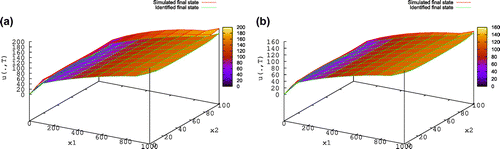
Figure 2. (a) $V_1=0.01$, $D_L=60$: Error 0.10 (b) $V_1=0.01$, $D_L=20$: Error 0.22.

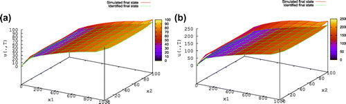
The numerical results presented in Figures 1 and 2 show that the procedure described in (51(51) $$\begin{array}{c}\hfill \begin{array}{cc}{\mathit{\partial }}_t\mathbf{u}-\mathrm{d}iv(D\mathrm{\nabla }\mathbf{u})+\mathit{\rho }\mathbf{u}=0\hfill & \text{in}\mathrm{\Omega }\times (T^{\ast },T)\hfill \\ \mathbf{u}(·,T^{\ast })\in L^2(\mathrm{\Omega })\hfill & \text{in}\mathrm{\Omega }\hfill \\ \mathbf{u}=0\hfill & \text{on}{\mathrm{\Gamma }}_{\text{in}}\times (T^{\ast },T)\hfill \\ {\displaystyle (D\mathrm{\nabla }\mathbf{u}+\frac{1}{2}\mathbf{u}V)·\mathit{\nu }=0}\hfill & \text{on}({\mathrm{\Gamma }}_L\cup {\mathrm{\Gamma }}_{out})\times (T^{\ast },T)\hfill \end{array}\end{array}$$(51) )–(56(56) $$\begin{array}{c}\hfill u(x,T)\approx e^{-\frac{1}{2}\mathit{\psi }(x)}\sum _{k=0}^K{y}_k{e}_k(x),x\in \mathrm{\Omega }\end{array}$$(56) ) identifies accurately the final state $u(·,T)$ in $\mathrm{\Omega }$ associated to the main problem (1(1) $$\begin{array}{c}\hfill L[u](x,t)=F(x,t)\text{in}\mathrm{\Omega }\times (0,T)\end{array}$$(1) )–(2(2) $$\begin{array}{c}\hfill L[u](x,t):={\mathit{\partial }}_{t}u(x,t)-\mathrm{d}iv(D(x)\mathrm{\nabla }u(x,t))+V(x)·\mathrm{\nabla }u(x,t)+Ru(x,t)\end{array}$$(2) ) and (23(23) $$\begin{array}{c}\hfill \begin{array}{c}u(·,0)=0\text{in}\mathrm{\Omega }\hfill \\ u=0\text{on}{\mathrm{\Gamma }}_{\text{in}}\times (0,T)\hfill \\ D\mathrm{\nabla }u·\mathit{\nu }=0\text{on}({\mathrm{\Gamma }}_{out}\cup {\mathrm{\Gamma }}_L)\times (0,T)\hfill \end{array}\end{array}$$(23) )–(24(24) $$\begin{array}{c}\hfill {\displaystyle F(x,t)=\sum _{n=1}^N{\mathit{\lambda }}_n(t)\mathit{\delta }(x-S_n)\text{in}\mathrm{\Omega }\times (0,T)}\end{array}$$(24) ). The analysis of those results indicates that the $L^2$ relative error on the identified final state depends on the dimensionless Peclet number $P_e=V_{1}L/(D_L+D_M)$. In fact, the reconstruction of $u(·,T)$ in $\mathrm{\Omega }$ is more accurate for smaller Peclet number.

Then, we apply the developed detection-identification method to identify the unknown elements $S_{n=1,\cdots ,N}$ and ${\mathit{\lambda }}_{n=1,\cdots ,N}$ defining in (24(24) $$\begin{array}{c}\hfill {\displaystyle F(x,t)=\sum _{n=1}^N{\mathit{\lambda }}_n(t)\mathit{\delta }(x-S_n)\text{in}\mathrm{\Omega }\times (0,T)}\end{array}$$(24) ) the sought source F occurring in $\mathrm{\Omega }=(0,L)\times (0,\ell )$ that generated the measurements M[F] given in (29(29) $$\begin{array}{c}\hfill M[F]:=\{D\mathrm{\nabla }u·\mathit{\nu }\text{on}\sum _{\text{in}};{\Vert V\Vert }_{2}u\text{on}\sum _L;(u,D\mathrm{\nabla }u·\mathit{\nu })\text{on}\sum _{i=1,\cdots ,N_{max}}\}\end{array}$$(29) ). To this end, we employ the developed active source detection procedure to go throughout $\mathrm{\Omega }$ by detecting for all $i=1,\cdots ,N_{max}$ whether there is or not an active source occurring in the subdomain ${\mathit{\omega }}_i=((i-1)\times 200,i\times 200)\times (0,\ell )$. Therefore, we compute for $i=1,\cdots ,N_{max}$ the Source Detection index ${SD}_i$ from (41(41) $$\begin{array}{c}\hfill {\displaystyle {SD}_i:=\frac{1}{T}{P}_1^i=\left\{\begin{array}{c}{\displaystyle \frac{1}{T}{\overline{\mathit{\lambda }}}_n\text{if}{S}_n\in {\mathit{\omega }}_i}\hfill \\ 0\text{otherwise}\hfill \end{array}\right.}\end{array}$$(41) )-(42(42) $$\begin{array}{cc}\hfill {\displaystyle P_1^i=e^{RT}{\int }_{{\mathit{\omega }}_i}u(x,T)\mathrm{d}x}& {\displaystyle +{\int }_{({\mathrm{\Gamma }}_{i-1}\cup {\mathrm{\Gamma }}_i)\times (0,T)}{e}^{Rt}(uV-D\mathrm{\nabla }u)·\mathit{\nu }\mathrm{d}x\mathrm{d}t}\hfill \\ \hfill & {\displaystyle +{\int }_{{\mathrm{\Gamma }}_L^i\times (0,T)}{e}^{Rt}uV·\mathit{\nu }\mathrm{d}x\mathrm{d}t}\hfill \end{array}$$(42) ) and determine as in (43(43) $$\begin{array}{c}\hfill {\displaystyle e^{-RT}{SD}_i\le e^{-R{T}^0}{SD}_i\le \frac{1}{\mathbf{T}}{\int }_0^{\mathbf{T}}{\mathit{\lambda }}_{\mathbf{n}}(\mathbf{t})\mathbf{dt}\le {SD}_i}\end{array}$$(43) ) the estimated lower and upper bounds of the mean value loaded by the unknwon intensity function ${\mathit{\lambda }}_n$ occurring in ${\mathit{\omega }}_i$. To carry out numerical experiments, we use $D_L=60m^2{s}^{-1}$, $V_1=0.01m{s}^{-1}$ and generate the simulated measurements M[F] defined in (29(29) $$\begin{array}{c}\hfill M[F]:=\{D\mathrm{\nabla }u·\mathit{\nu }\text{on}\sum _{\text{in}};{\Vert V\Vert }_{2}u\text{on}\sum _L;(u,D\mathrm{\nabla }u·\mathit{\nu })\text{on}\sum _{i=1,\cdots ,N_{max}}\}\end{array}$$(29) ) using $N=3$ point sources loading the time-dependent intensity functions ${\mathit{\lambda }}_{n=1,\cdots ,3}$ introduced in (63(63) $$\begin{array}{c}\hfill {\displaystyle {\mathit{\lambda }}_1(t)={\mathit{\chi }}_{(\frac{T^0}{5},T^0)}(t),{\mathit{\lambda }}_2(t)=\frac{4}{{T^0}^2}t(T^0-t)\text{and}{\mathit{\lambda }}_3(t)=\sum _{k=1}^3{c}_k{e}^{-v_k{(t-{\mathit{\tau }}_k)}^2}}\end{array}$$(63) ) for different source locations $S_{n=1,2,3}$. As far as the obtained numerical results are concerned, we present in a same table for each simulated measurements the computed Source Detection index ${SD}_i$ in ${\mathit{\omega }}_i$ for $i=1,\cdots ,N_{max}=4$, the interval $[{SD}_i{e}^{-RT};{SD}_i]$ obtained in (43(43) $$\begin{array}{c}\hfill {\displaystyle e^{-RT}{SD}_i\le e^{-R{T}^0}{SD}_i\le \frac{1}{\mathbf{T}}{\int }_0^{\mathbf{T}}{\mathit{\lambda }}_{\mathbf{n}}(\mathbf{t})\mathbf{dt}\le {SD}_i}\end{array}$$(43) ) and the corresponding mean value of the intensity function ${\mathit{\lambda }}_n$, used for simulation, computed from (64(64) $$\begin{array}{c}\hfill \begin{array}{c}{\displaystyle \frac{1}{T}{\int }_0^T{\mathit{\lambda }}_1(t)\mathrm{d}t=\frac{4T^0}{5T},\frac{1}{T}{\int }_0^T{\mathit{\lambda }}_2(t)\mathrm{d}t=\frac{2T^0}{3T}\text{and}}\hfill \\ {\displaystyle \frac{1}{T}{\int }_0^T{\mathit{\lambda }}_3(t)\mathrm{d}t=\frac{\sqrt{\mathit{\pi }}}{2T}{\sum }_{k=1}^3\frac{c_k}{\sqrt{v_k}}(\mathrm{e}rf(\sqrt{v_k}(T^0-{\mathit{\tau }}_k))-\mathrm{e}rf(-\sqrt{v_k}{\mathit{\tau }}_k))}\hfill \end{array}\end{array}$$(64) ) for $T^0=(3/4)T$. We give in the caption of each table the three source positions $S_{n=1,2,3}$ used to generate the simulations.

Table 1. Source Detection: simulation with $S_1=(300,50);S_2=(500,70);S_3=(700,30)$.

${\mathit{\omega }}_i=((i-1)\times 200,i\times 200)\times (0,\ell )$	${\mathit{\omega }}_1$	${\mathit{\omega }}_2$	${\mathit{\omega }}_3$	${\mathit{\omega }}_4$
Source Detection index: ${SD}_i$	0.026	0.672	0.538	0.233
$[{SD}_i{e}^{-RT};{SD}_i]$	[0.022; 0.026]	[0.581; 0.672]	[0.466; 0.538]	[0.201; 0.233]
$\frac{1}{T}{\int }_0^T{\mathit{\lambda }}_n(t)\mathrm{d}t$ used for simulation	No occurring source	0.60	0.50	0.228

Table 2. Source Detection: simulation with $S_1=(100,50);S_2=(500,70);S_3=(700,30)$.

${\mathit{\omega }}_i=((i-1)\times 200,i\times 200)\times (0,\ell )$	${\mathit{\omega }}_1$	${\mathit{\omega }}_2$	${\mathit{\omega }}_3$	${\mathit{\omega }}_4$
Source Detection index: ${SD}_i$	0.669	0.017	0.544	0.233
$[{SD}_i{e}^{-RT};{SD}_i]$	[0.579; 0.669]	[0.015; 0.017]	[0.471; 0.544]	[0.201; 0.233]
$\frac{1}{T}{\int }_0^T{\mathit{\lambda }}_n(t)\mathrm{d}t$ used for simulation	0.60	No occurring source	0.50	0.228

Table 3. Source Detection: simulation with $S_1=(100,50);S_2=(300,70);S_3=(700,30)$.

${\mathit{\omega }}_i=((i-1)\times 200,i\times 200)\times (0,\ell )$	${\mathit{\omega }}_1$	${\mathit{\omega }}_2$	${\mathit{\omega }}_3$	${\mathit{\omega }}_4$
Source Detection index: ${SD}_i$	0.679	0.555	1.31E-04	0.233
$[{SD}_i{e}^{-RT};{SD}_i]$	[0.588; 0.679]	[0.481; 0.555]	[0.00011; 0.00013]	[0.201; 0.233]
$\frac{1}{T}{\int }_0^T{\mathit{\lambda }}_n(t)\mathrm{d}t$ used for simulation	0.60	0.50	No occurring source	0.228

Table 4. Source Detection: simulation with $S_1=(100,50);S_2=(300,70);S_3=(500,30)$.

${\mathit{\omega }}_i=((i-1)\times 200,i\times 200)\times (0,\ell )$	${\mathit{\omega }}_1$	${\mathit{\omega }}_2$	${\mathit{\omega }}_3$	${\mathit{\omega }}_4$
Source Detection index: ${SD}_i$	0.682	0.562	0.247	0.018
$[{SD}_i{e}^{-RT};{SD}_i]$	[0.591; 0.682]	[0.487; 0.562]	[0.214; 0.247]	[0.015; 0.018]
$\frac{1}{T}{\int }_0^T{\mathit{\lambda }}_n(t)\mathrm{d}t$ used for simulation	0.60	0.50	0.228	No occurring source

The analysis of the numerical experiments presented in Tables 1–4 shows that the developed active source detection procedure determines accurately throughout the monitored domain $\mathrm{\Omega }$ whether there is or not an active source occurring in each ${\mathit{\omega }}_{i=1,\cdots ,N_{max}}\subset \mathrm{\Omega }$. Furthermore, in view of (43(43) $$\begin{array}{c}\hfill {\displaystyle e^{-RT}{SD}_i\le e^{-R{T}^0}{SD}_i\le \frac{1}{\mathbf{T}}{\int }_0^{\mathbf{T}}{\mathit{\lambda }}_{\mathbf{n}}(\mathbf{t})\mathbf{dt}\le {SD}_i}\end{array}$$(43) ) this procedure provides estimated lower and upper bounds ${SD}_i{e}^{-RT}$ and ${SD}_i$ of the mean value loaded by the unknwon time-dependent intensity function ${\mathit{\lambda }}_n$ of the deceted source occurring in ${\mathit{\omega }}_i$. In Tables 1–4, the two estimated frame bounds appear to be accurate and yield an approximation of the mean value loaded by the unknown time-dependent intensity function ${\mathit{\lambda }}_n$ without having to identify its historic.

Besides, once an active time-dependent point source is detected in ${\mathit{\omega }}_i\subset \mathrm{\Omega }$ where $i\in \{1,\cdots ,N_{max}\}$, we employ the developed identification procedure to localize its position $S_n$ from (47(47) $$\begin{array}{c}\hfill {\displaystyle \mathit{\psi }(S_n)=\mathrm{l}n\left({\displaystyle \frac{P_{e^{\mathit{\psi }}}^i}{P_1^i}}\right)\text{and}{\mathit{\psi }}^{\perp }(S_n)=\frac{P_{{\mathit{\psi }}^{\perp }}^i}{P_1^i}\iff \mathrm{\Psi }(S_n)=\left(\begin{array}{c}{\displaystyle \mathrm{l}n(\frac{P_{e^{\mathit{\psi }}}^i}{P_1^i})}\\ {\displaystyle \frac{P_{{\mathit{\psi }}^{\perp }}^i}{P_1^i}}\end{array}\right)}\end{array}$$(47) )-(50(50) $$\begin{array}{c}\hfill x^{k+1}=x^k-J_{\mathrm{\Psi }}^{-1}(x^k)\left(\begin{array}{c}{\displaystyle \mathit{\psi }(x_k)-\mathrm{l}n(\frac{P_{e^{\mathit{\psi }}}^i}{P_1^i})}\\ {\displaystyle {\mathit{\psi }}^{\perp }(x_k)-\frac{P_{{\mathit{\psi }}^{\perp }}^i}{P_1^i}}\end{array}\right),k\ge 0\end{array}$$(50) ) and to identify its time-dependent intensity function ${\mathit{\lambda }}_n$ using the recursive formula (60(60) $$\begin{array}{c}\hfill {\displaystyle {\mathit{\lambda }}_n^m=\frac{1}{v(S_n,t_1)}\left(\frac{Q_{t_{m+1}}^i}{\mathrm{\Delta }t}-\sum _{k=1}^{m-1}{\mathit{\lambda }}_n^{k}v(S_n,t_{m+1-k})\right),\text{for all}m\ge 1}\end{array}$$(60) ). To carry out numerical experiments, we use for example the simulations M[F] generated for the experiments in Table 4. Since the results of the detection procedure presented in Table 4 indicate that the involved sources are occurring in ${\mathit{\omega }}_i$ for $i=1,\cdots ,3$ then, we apply the identification procedure to determine for each $i=1,\cdots ,3$ the two unknown elements ${\mathit{\lambda }}_n$ and $S_n$ defining the detected source occurring in ${\mathit{\omega }}_i$. To this end, we compute for $i=1,\cdots ,3$ the coefficients $P_1^i$, $P_{e^{\mathit{\psi }}}^i$, $P_{{\mathit{\psi }}^{\perp }}^i$ from (42(42) $$\begin{array}{cc}\hfill {\displaystyle P_1^i=e^{RT}{\int }_{{\mathit{\omega }}_i}u(x,T)\mathrm{d}x}& {\displaystyle +{\int }_{({\mathrm{\Gamma }}_{i-1}\cup {\mathrm{\Gamma }}_i)\times (0,T)}{e}^{Rt}(uV-D\mathrm{\nabla }u)·\mathit{\nu }\mathrm{d}x\mathrm{d}t}\hfill \\ \hfill & {\displaystyle +{\int }_{{\mathrm{\Gamma }}_L^i\times (0,T)}{e}^{Rt}uV·\mathit{\nu }\mathrm{d}x\mathrm{d}t}\hfill \end{array}$$(42) ) and (46(46) $$\begin{array}{c}\hfill \begin{array}{c}{\displaystyle P_{e^{\mathit{\psi }}}^i=e^{RT}{\int }_{{\mathit{\omega }}_i}{e}^{\mathit{\psi }}u(x,T)\mathrm{d}x-{\int }_{({\mathrm{\Gamma }}_{i-1}\cup {\mathrm{\Gamma }}_i)\times (0,T)}{e}^{\mathit{\psi }+Rt}D\mathrm{\nabla }u·\mathit{\nu }\mathrm{d}x\mathrm{d}t}\hfill \\ {\displaystyle P_{{\mathit{\psi }}^{\perp }}^i=e^{RT}{\int }_{{\mathit{\omega }}_i}{\mathit{\psi }}^{\perp }u(x,T)\mathrm{d}x+{\int }_{({\mathrm{\Gamma }}_{i-1}\cup {\mathrm{\Gamma }}_i)\times (0,T)}{e}^{Rt}(u[{\mathit{\psi }}^{\perp }V-V^{\perp }]-{\mathit{\psi }}^{\perp }D\mathrm{\nabla }u)·\mathit{\nu }\mathrm{d}x\mathrm{d}t}\hfill \\ {\displaystyle +{\int }_{{\mathrm{\Gamma }}_L^i\times (0,T)}{e}^{Rt}u({\mathit{\psi }}^{\perp }V-V^{\perp })·\mathit{\nu }\mathrm{d}x\mathrm{d}t}\hfill \end{array}\end{array}$$(46) ). Then, according to (47(47) $$\begin{array}{c}\hfill {\displaystyle \mathit{\psi }(S_n)=\mathrm{l}n\left({\displaystyle \frac{P_{e^{\mathit{\psi }}}^i}{P_1^i}}\right)\text{and}{\mathit{\psi }}^{\perp }(S_n)=\frac{P_{{\mathit{\psi }}^{\perp }}^i}{P_1^i}\iff \mathrm{\Psi }(S_n)=\left(\begin{array}{c}{\displaystyle \mathrm{l}n(\frac{P_{e^{\mathit{\psi }}}^i}{P_1^i})}\\ {\displaystyle \frac{P_{{\mathit{\psi }}^{\perp }}^i}{P_1^i}}\end{array}\right)}\end{array}$$(47) ) and in view of (62(62) $$\begin{array}{c}\hfill \mathrm{\Psi }(x)=\left(\begin{array}{cc}{\displaystyle -\frac{V_1}{D_M+D_L}{x}_1}& \\ \\ {\displaystyle -\frac{V_1}{D_M+D_T}{x}_2}\end{array}\right)\end{array}$$(62) ), the two unknown coordinates $S_{n_{x_1}}$ and $S_{n_{x_2}}$ defining the position $S_n$ of the detected source occurring in ${\mathit{\omega }}_i$ are localized as follows:(70) $$\begin{array}{c}\hfill \begin{array}{c}{\displaystyle S_{n_{x_1}}=-\frac{D_L+D_M}{V_1}\mathrm{l}n\left({\displaystyle \frac{P_{e^{\mathit{\psi }}}^i}{P_1^i}}\right)}\hfill \\ {\displaystyle S_{n_{x_2}}=-\frac{D_T+D_M}{V_1}\frac{P_{{\mathit{\psi }}^{\perp }}^i}{P_1^i}}\hfill \end{array}\end{array}$$(70)

Furthermore, using the localized source position $S_n$ we identify its time-dependent intensity function ${\mathit{\lambda }}_n$ from (60(60) $$\begin{array}{c}\hfill {\displaystyle {\mathit{\lambda }}_n^m=\frac{1}{v(S_n,t_1)}\left(\frac{Q_{t_{m+1}}^i}{\mathrm{\Delta }t}-\sum _{k=1}^{m-1}{\mathit{\lambda }}_n^{k}v(S_n,t_{m+1-k})\right),\text{for all}m\ge 1}\end{array}$$(60) ). To this end, we need to solve the boundary control problem introduced in (31(31) $$\begin{array}{cc}& \begin{array}{cc}{\mathit{\partial }}_{t}v-\mathrm{d}iv(D\mathrm{\nabla }v)-V·\mathrm{\nabla }v+Rv=0\hfill & \text{in}\mathrm{\Omega }\times (0,T)\hfill \\ v(·,0)=0\hfill & \text{in}\mathrm{\Omega }\hfill \\ v={\mathit{\gamma }}_{\text{in}}\hfill & \text{on}{\mathrm{\Gamma }}_{\text{in}}\times (0,T)\hfill \\ (D\mathrm{\nabla }v+vV)·\mathit{\nu }=0\hfill & \text{on}{\mathrm{\Gamma }}_L\times (0,T)\hfill \\ (D\mathrm{\nabla }v+vV)·\mathit{\nu }={\mathit{\gamma }}_{out}\hfill & \text{on}{\mathrm{\Gamma }}_{out}\times (0,T)\hfill \end{array}\hfill \end{array}$$(31) )–(32(32) $$\begin{array}{cc}& \text{such that:}v(x^{\ast },·)\ne 0\text{a.e. in}(0,T)\hfill \end{array}$$(32) ) for $x^{\ast }=S_n$. By considering the following adjoint problem:(71) $$\begin{array}{c}\hfill \begin{array}{cc}-{\mathit{\partial }}_t\mathit{\xi }-\mathrm{d}iv(D\mathrm{\nabla }\mathit{\xi })+V·\mathrm{\nabla }\mathit{\xi }+R\mathit{\xi }=\mathit{\delta }(x-S_n)\hfill & \text{in}\mathrm{\Omega }\times (0,T)\hfill \\ \mathit{\xi }(·,T)=0\hfill & \text{in}\mathrm{\Omega }\hfill \\ \mathit{\xi }=0\hfill & \text{on}{\mathrm{\Gamma }}_{\text{in}}\times (0,T)\hfill \\ D\mathrm{\nabla }\mathit{\xi }·\mathit{\nu }=0\hfill & \text{on}({\mathrm{\Gamma }}_L\cup {\mathrm{\Gamma }}_{\text{out}})\times (0,T)\hfill \end{array}\end{array}$$(71)

and using similar techniques as in [13] it follows that setting ${\mathit{\gamma }}_{\text{in}}=-D\mathrm{\nabla }\mathit{\xi }·\mathit{\nu }$ on ${\mathrm{\Gamma }}_{\text{in}}\times (0,T)$ and ${\mathit{\gamma }}_{\text{out}}=\mathit{\xi }$ on ${\mathrm{\Gamma }}_{\text{out}}\times (0,T)$ leads the solution of the problem (31(31) $$\begin{array}{cc}& \begin{array}{cc}{\mathit{\partial }}_{t}v-\mathrm{d}iv(D\mathrm{\nabla }v)-V·\mathrm{\nabla }v+Rv=0\hfill & \text{in}\mathrm{\Omega }\times (0,T)\hfill \\ v(·,0)=0\hfill & \text{in}\mathrm{\Omega }\hfill \\ v={\mathit{\gamma }}_{\text{in}}\hfill & \text{on}{\mathrm{\Gamma }}_{\text{in}}\times (0,T)\hfill \\ (D\mathrm{\nabla }v+vV)·\mathit{\nu }=0\hfill & \text{on}{\mathrm{\Gamma }}_L\times (0,T)\hfill \\ (D\mathrm{\nabla }v+vV)·\mathit{\nu }={\mathit{\gamma }}_{out}\hfill & \text{on}{\mathrm{\Gamma }}_{out}\times (0,T)\hfill \end{array}\hfill \end{array}$$(31) ) to yield the assertion (32(32) $$\begin{array}{cc}& \text{such that:}v(x^{\ast },·)\ne 0\text{a.e. in}(0,T)\hfill \end{array}$$(32) ) for $x^{\ast }=S_n$. We present the obtained identification results for the three detected sources in Table 4 while introducing a Gaussian noise on the used simulations. We give for each introduced intensity noise the three identified source positions and present on a same graphic for each involved source, the intensity function used for simulation given in (63(63) $$\begin{array}{c}\hfill {\displaystyle {\mathit{\lambda }}_1(t)={\mathit{\chi }}_{(\frac{T^0}{5},T^0)}(t),{\mathit{\lambda }}_2(t)=\frac{4}{{T^0}^2}t(T^0-t)\text{and}{\mathit{\lambda }}_3(t)=\sum _{k=1}^3{c}_k{e}^{-v_k{(t-{\mathit{\tau }}_k)}^2}}\end{array}$$(63) ) and the identified intensity computed from (60(60) $$\begin{array}{c}\hfill {\displaystyle {\mathit{\lambda }}_n^m=\frac{1}{v(S_n,t_1)}\left(\frac{Q_{t_{m+1}}^i}{\mathrm{\Delta }t}-\sum _{k=1}^{m-1}{\mathit{\lambda }}_n^{k}v(S_n,t_{m+1-k})\right),\text{for all}m\ge 1}\end{array}$$(60) ). We indicate also for each drawing the $L^2$-relative error computed from $\Vert {\mathit{\lambda }}_{\text{simulation}}-{\mathit{\lambda }}_{\text{identified}}{\Vert }_{L^2(0,T)}/{\Vert {\mathit{\lambda }}_{\text{simulation}}\Vert }_{L^2(0,T)}$.

Figure 3. (a) Gaussian noise $5\%$: Error 0.253 (b) Gaussian noise $10\%$: Error 0.301.

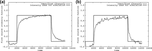
Figure 4. (a) Gaussian noise $5\%$: Error 0.141 (b) Gaussian noise $10\%$: Error 0.221.

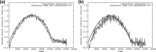
Figure 5. (a) Gaussian noise $5\%$: Error 0.191 (b) Gaussian noise $10\%$: Error 0.321.

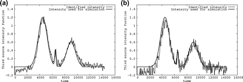
The identified source positions are as follows: For a Gaussian noise $5\%$, we obtained $S_1=(97.31,48.3)$, $S_2=(303.4,65.7)$ and $S_3=(498.2,27.4)$. For a Gaussian noise $10\%$, we found $S_1=(112.61,39.8)$, $S_2=(309.2,78.4)$ and $S_3=(506.2,37.5)$.

The numerical results obtained for the localization of the sought source positions as well as for the identification of their unknown time-dependent intensity functions presented in Figures 3–5 show that the developed identification procedure determines accurately the unknown elements defining the occurring sources and is relatively stable with respect to the introduction of a Gaussian noise on the used measurements.

6. Conclusion and outlook

We addressed the non-linear inverse source problem of identifying multiple unknown time-dependent point sources occurring in a two-dimensional evolution advection–dispersion–reaction equation. We developed a source detection procedure that goes throughout the monitored domain to detect the presence of all occurring active sources. Once a source is detected, this procedure determines lower and upper bounds of the mean value discharged by its unknown time-dependent intensity function without having to identify the historic of this latest. In practice, this procedure leads to decide whether to go further with the identification of a detected source or to consider that it is not a significant source since the mean value discharged by its unknown intensity function remains below a certain tolerance/criterion. Then, we developed an identification method that localizes the sought position of a detected source as the unique solution of an equation satisfied by the introduced dispersion-current function and identifies its intensity function from solving an associated deconvolution problem. Some numerical experiments on a variant of the surface water BOD pollution model were carried out. The obtained numerical results show that the developed detection–identification method is accurate and relatively stable with respect to the introduction of a Gaussian noise on the used measurements.

6.1. Outlook

We carried out some numerical experiments where the assumption (28(28) $$\begin{array}{c}\hfill \forall i=1,\cdots ,N_{max},\text{there exists}\underline{atmost}\text{one element}n\in \{1,\cdots ,N\}/S_n\in {\mathit{\omega }}_i\end{array}$$(28) ) is not respected. That is we considered a domain $\mathrm{\Omega }$ containing an only one suspected zone ${\mathit{\omega }}_1$ i.e. $N_{max}=1$ where multiple point sources could occur. Then, we applied the detection–identification method using measurements generated firstly by one, secondly by two and thirdly by three point sources occurring in ${\mathit{\omega }}_1$ by discharging three different positive constants. The obtained numerical results are as follows: in the case of one point source: the localized position $S_n$ and ${\overline{\mathit{\lambda }}}_n$ are accurate. In the case of two point sources: the localized position $S_n$ is between the two involved source positions. In the case of three point sources: the localized position $S_n$ is in the triangle of summits the three involved source positions. Moreover, in these two last cases, the localized position $S_n$ seems to be nearer to the source position of biggest discharge constant. However, in all cases the determined ${\overline{\mathit{\lambda }}}_n$ corresponds to the sum of all discharged amounts.

Although it is expected, as in (41(41) $$\begin{array}{c}\hfill {\displaystyle {SD}_i:=\frac{1}{T}{P}_1^i=\left\{\begin{array}{c}{\displaystyle \frac{1}{T}{\overline{\mathit{\lambda }}}_n\text{if}{S}_n\in {\mathit{\omega }}_i}\hfill \\ 0\text{otherwise}\hfill \end{array}\right.}\end{array}$$(41) )–(42(42) $$\begin{array}{cc}\hfill {\displaystyle P_1^i=e^{RT}{\int }_{{\mathit{\omega }}_i}u(x,T)\mathrm{d}x}& {\displaystyle +{\int }_{({\mathrm{\Gamma }}_{i-1}\cup {\mathrm{\Gamma }}_i)\times (0,T)}{e}^{Rt}(uV-D\mathrm{\nabla }u)·\mathit{\nu }\mathrm{d}x\mathrm{d}t}\hfill \\ \hfill & {\displaystyle +{\int }_{{\mathrm{\Gamma }}_L^i\times (0,T)}{e}^{Rt}uV·\mathit{\nu }\mathrm{d}x\mathrm{d}t}\hfill \end{array}$$(42) ), that the computed ${\overline{\mathit{\lambda }}}_n$ corresponds to the sum of all amounts discharged by the different involved point sources, it is not clear whether the localized source position is always in the polygon of summits the occurring source positions. An outlook of the present study could be to investigate this claim which would give another application of the developed detection–identification method: to be applied on a monitored domain $\mathrm{\Omega }$ containing suspected zones ${\mathit{\omega }}_i$ where multiple time-dependent point sources of known positions could occur. Then, the method determines the total amount discharged by all sources occurring in ${\mathit{\omega }}_i$. The localized position would be interpreted as follows: (1) if it coincides with one among the already known positions then, it is the unique source responsible of the detected pollution; (2) If it is in a polygon of summits some of the known source positions then, there were more than one active source among the already known positions (the number of active sources is it the number of summits?); (3) Otherwise, the responsable of the detected pollution is rather a new unknown source(s).

Notes

No potential conflict of interest was reported by the authors.

Appendix 1

Here, we establish the proof of Proposition 4.2:

In view of [28], we consider the null controllability problem of determining a distributed control $\mathit{\gamma }\in L^2({\mathit{\omega }}_{N_{max}+1}\times (T^{\ast },T))$ that to a given initial state ${\mathit{\phi }}_0\in L^2(\mathrm{\Omega })$ drives the solution $\mathit{\phi }$ of the following system:(A1) $$\begin{array}{cc}& \begin{array}{cc}{\mathit{\partial }}_t\mathit{\phi }-\mathrm{d}iv(D\mathrm{\nabla }\mathit{\phi })+\mathit{\rho }\mathit{\phi }=\mathit{\gamma }(x,t){\mathit{\chi }}_{{\mathit{\omega }}_{N_{max}+1}}(x)\hfill & \text{in}\mathrm{\Omega }\times (T^{\ast },T)\hfill \\ \mathit{\phi }(·,T^{\ast })={\mathit{\phi }}_0\hfill & \text{in}\mathrm{\Omega }\hfill \\ \mathit{\phi }=0\hfill & \text{on}{\mathrm{\Gamma }}_{\text{in}}\times (T^{\ast },T)\hfill \\ {\displaystyle (D\mathrm{\nabla }\mathit{\phi }+\frac{1}{2}\mathit{\phi }V)·\mathit{\nu }=0}\hfill & \text{on}({\mathrm{\Gamma }}_L\cup {\mathrm{\Gamma }}_{\text{out}})\times (T^{\ast },T)\hfill \end{array}\hfill \end{array}$$(A1) (A2) $$\begin{array}{cc}& \text{to the final state:}\mathit{\phi }(·,T)=0\text{in}\mathrm{\Omega }\hfill \end{array}$$(A2)

where ${\mathit{\chi }}_{{\mathit{\omega }}_{N_{max}+1}}$ is the characteristic function of ${\mathit{\omega }}_{N_{max}+1}\subset \mathrm{\Omega }$. Multiplying the first equation in (A1(A1) $$\begin{array}{cc}& \begin{array}{cc}{\mathit{\partial }}_t\mathit{\phi }-\mathrm{d}iv(D\mathrm{\nabla }\mathit{\phi })+\mathit{\rho }\mathit{\phi }=\mathit{\gamma }(x,t){\mathit{\chi }}_{{\mathit{\omega }}_{N_{max}+1}}(x)\hfill & \text{in}\mathrm{\Omega }\times (T^{\ast },T)\hfill \\ \mathit{\phi }(·,T^{\ast })={\mathit{\phi }}_0\hfill & \text{in}\mathrm{\Omega }\hfill \\ \mathit{\phi }=0\hfill & \text{on}{\mathrm{\Gamma }}_{\text{in}}\times (T^{\ast },T)\hfill \\ {\displaystyle (D\mathrm{\nabla }\mathit{\phi }+\frac{1}{2}\mathit{\phi }V)·\mathit{\nu }=0}\hfill & \text{on}({\mathrm{\Gamma }}_L\cup {\mathrm{\Gamma }}_{\text{out}})\times (T^{\ast },T)\hfill \end{array}\hfill \end{array}$$(A1) ) by $\mathit{\xi }$ the solution of the adjoint problem that to a given ${\mathit{\xi }}_0\in L^2(\mathrm{\Omega })$ associates(A3) $$\begin{array}{c}\hfill \begin{array}{cc}-{\mathit{\partial }}_t\mathit{\xi }-\mathrm{d}iv(D\mathrm{\nabla }\mathit{\xi })+\mathit{\rho }\mathit{\xi }=0\hfill & \text{in}\mathrm{\Omega }\times (T^{\ast },T)\hfill \\ \mathit{\xi }(·,T)={\mathit{\xi }}_0\hfill & \text{in}\mathrm{\Omega }\hfill \\ \mathit{\xi }=0\hfill & \text{on}{\mathrm{\Gamma }}_{\text{in}}\times (T^{\ast },T)\hfill \\ {\displaystyle (D\mathrm{\nabla }\mathit{\xi }+\frac{1}{2}\mathit{\xi }V)·\mathit{\nu }=0}\hfill & \text{on}({\mathrm{\Gamma }}_L\cup {\mathrm{\Gamma }}_{\text{out}})\times (T^{\ast },T)\hfill \end{array}\end{array}$$(A3)

and integrating by parts over $\mathrm{\Omega }\times (T^{\ast },T)$ using Green’s formula gives(A4) $$\begin{array}{c}\hfill {\displaystyle {\int }_{{\mathit{\omega }}_{N_{max}+1}\times (T^{\ast },T)}\mathit{\xi }\mathit{\gamma }\mathrm{d}x\mathrm{d}t={\int }_{\mathrm{\Omega }}[\mathit{\phi }(x,t)\mathit{\xi }(x,t){]}_{T^{\ast }}^T\mathrm{d}x,\forall {\mathit{\xi }}_0\in L^2(\mathrm{\Omega })}\end{array}$$(A4)

Therefore, a distributed control $\mathit{\gamma }\in L^2({\mathit{\omega }}_{N_{max}+1}\times (T^{\ast },T))$ solves the null controllability problem introduced in (A1(A1) $$\begin{array}{cc}& \begin{array}{cc}{\mathit{\partial }}_t\mathit{\phi }-\mathrm{d}iv(D\mathrm{\nabla }\mathit{\phi })+\mathit{\rho }\mathit{\phi }=\mathit{\gamma }(x,t){\mathit{\chi }}_{{\mathit{\omega }}_{N_{max}+1}}(x)\hfill & \text{in}\mathrm{\Omega }\times (T^{\ast },T)\hfill \\ \mathit{\phi }(·,T^{\ast })={\mathit{\phi }}_0\hfill & \text{in}\mathrm{\Omega }\hfill \\ \mathit{\phi }=0\hfill & \text{on}{\mathrm{\Gamma }}_{\text{in}}\times (T^{\ast },T)\hfill \\ {\displaystyle (D\mathrm{\nabla }\mathit{\phi }+\frac{1}{2}\mathit{\phi }V)·\mathit{\nu }=0}\hfill & \text{on}({\mathrm{\Gamma }}_L\cup {\mathrm{\Gamma }}_{\text{out}})\times (T^{\ast },T)\hfill \end{array}\hfill \end{array}$$(A1) )–(A2(A2) $$\begin{array}{cc}& \text{to the final state:}\mathit{\phi }(·,T)=0\text{in}\mathrm{\Omega }\hfill \end{array}$$(A2) ) if and only if it yields(A5) $$\begin{array}{c}\hfill {\displaystyle {\int }_{{\mathit{\omega }}_{N_{max}+1}\times (T^{\ast },T)}\mathit{\xi }\mathit{\gamma }\mathrm{d}x\mathrm{d}t=-{\int }_{\mathrm{\Omega }}\mathit{\phi }(x,T^{\ast })\mathit{\xi }(x,T^{\ast })\mathrm{d}x,\forall {\mathit{\xi }}_0\in L^2(\mathrm{\Omega })}\end{array}$$(A5)

The necessary condition in (A5(A5) $$\begin{array}{c}\hfill {\displaystyle {\int }_{{\mathit{\omega }}_{N_{max}+1}\times (T^{\ast },T)}\mathit{\xi }\mathit{\gamma }\mathrm{d}x\mathrm{d}t=-{\int }_{\mathrm{\Omega }}\mathit{\phi }(x,T^{\ast })\mathit{\xi }(x,T^{\ast })\mathrm{d}x,\forall {\mathit{\xi }}_0\in L^2(\mathrm{\Omega })}\end{array}$$(A5) ) is implied by (A4(A4) $$\begin{array}{c}\hfill {\displaystyle {\int }_{{\mathit{\omega }}_{N_{max}+1}\times (T^{\ast },T)}\mathit{\xi }\mathit{\gamma }\mathrm{d}x\mathrm{d}t={\int }_{\mathrm{\Omega }}[\mathit{\phi }(x,t)\mathit{\xi }(x,t){]}_{T^{\ast }}^T\mathrm{d}x,\forall {\mathit{\xi }}_0\in L^2(\mathrm{\Omega })}\end{array}$$(A4) ) whereas the sufficient condition is obtained from observing that if the solution $\mathit{\phi }$ of (A1(A1) $$\begin{array}{cc}& \begin{array}{cc}{\mathit{\partial }}_t\mathit{\phi }-\mathrm{d}iv(D\mathrm{\nabla }\mathit{\phi })+\mathit{\rho }\mathit{\phi }=\mathit{\gamma }(x,t){\mathit{\chi }}_{{\mathit{\omega }}_{N_{max}+1}}(x)\hfill & \text{in}\mathrm{\Omega }\times (T^{\ast },T)\hfill \\ \mathit{\phi }(·,T^{\ast })={\mathit{\phi }}_0\hfill & \text{in}\mathrm{\Omega }\hfill \\ \mathit{\phi }=0\hfill & \text{on}{\mathrm{\Gamma }}_{\text{in}}\times (T^{\ast },T)\hfill \\ {\displaystyle (D\mathrm{\nabla }\mathit{\phi }+\frac{1}{2}\mathit{\phi }V)·\mathit{\nu }=0}\hfill & \text{on}({\mathrm{\Gamma }}_L\cup {\mathrm{\Gamma }}_{\text{out}})\times (T^{\ast },T)\hfill \end{array}\hfill \end{array}$$(A1) ) with a given $\mathit{\gamma }\in L^2({\mathit{\omega }}_{N_{max}+1}\times (T^{\ast },T))$ satisfies (A5(A5) $$\begin{array}{c}\hfill {\displaystyle {\int }_{{\mathit{\omega }}_{N_{max}+1}\times (T^{\ast },T)}\mathit{\xi }\mathit{\gamma }\mathrm{d}x\mathrm{d}t=-{\int }_{\mathrm{\Omega }}\mathit{\phi }(x,T^{\ast })\mathit{\xi }(x,T^{\ast })\mathrm{d}x,\forall {\mathit{\xi }}_0\in L^2(\mathrm{\Omega })}\end{array}$$(A5) ) then, from (A4(A4) $$\begin{array}{c}\hfill {\displaystyle {\int }_{{\mathit{\omega }}_{N_{max}+1}\times (T^{\ast },T)}\mathit{\xi }\mathit{\gamma }\mathrm{d}x\mathrm{d}t={\int }_{\mathrm{\Omega }}[\mathit{\phi }(x,t)\mathit{\xi }(x,t){]}_{T^{\ast }}^T\mathrm{d}x,\forall {\mathit{\xi }}_0\in L^2(\mathrm{\Omega })}\end{array}$$(A4) ) we get ${\int }_{\mathrm{\Omega }}\mathit{\phi }(·,T){\mathit{\xi }}_0\mathrm{d}x=0$ for all ${\mathit{\xi }}_0\in L^2(\mathrm{\Omega })$. That leads to $\mathit{\phi }(·,T)=0$ in $\mathrm{\Omega }$ and thus, $\mathit{\gamma }$ solves the null controllability problem (A1(A1) $$\begin{array}{cc}& \begin{array}{cc}{\mathit{\partial }}_t\mathit{\phi }-\mathrm{d}iv(D\mathrm{\nabla }\mathit{\phi })+\mathit{\rho }\mathit{\phi }=\mathit{\gamma }(x,t){\mathit{\chi }}_{{\mathit{\omega }}_{N_{max}+1}}(x)\hfill & \text{in}\mathrm{\Omega }\times (T^{\ast },T)\hfill \\ \mathit{\phi }(·,T^{\ast })={\mathit{\phi }}_0\hfill & \text{in}\mathrm{\Omega }\hfill \\ \mathit{\phi }=0\hfill & \text{on}{\mathrm{\Gamma }}_{\text{in}}\times (T^{\ast },T)\hfill \\ {\displaystyle (D\mathrm{\nabla }\mathit{\phi }+\frac{1}{2}\mathit{\phi }V)·\mathit{\nu }=0}\hfill & \text{on}({\mathrm{\Gamma }}_L\cup {\mathrm{\Gamma }}_{\text{out}})\times (T^{\ast },T)\hfill \end{array}\hfill \end{array}$$(A1) )–(A2(A2) $$\begin{array}{cc}& \text{to the final state:}\mathit{\phi }(·,T)=0\text{in}\mathrm{\Omega }\hfill \end{array}$$(A2) ).

Besides, let $\widehat{\mathit{\xi }}$ be the solution of the adjoint problem introduced in (71(71) $$\begin{array}{c}\hfill \begin{array}{cc}-{\mathit{\partial }}_t\mathit{\xi }-\mathrm{d}iv(D\mathrm{\nabla }\mathit{\xi })+V·\mathrm{\nabla }\mathit{\xi }+R\mathit{\xi }=\mathit{\delta }(x-S_n)\hfill & \text{in}\mathrm{\Omega }\times (0,T)\hfill \\ \mathit{\xi }(·,T)=0\hfill & \text{in}\mathrm{\Omega }\hfill \\ \mathit{\xi }=0\hfill & \text{on}{\mathrm{\Gamma }}_{\text{in}}\times (0,T)\hfill \\ D\mathrm{\nabla }\mathit{\xi }·\mathit{\nu }=0\hfill & \text{on}({\mathrm{\Gamma }}_L\cup {\mathrm{\Gamma }}_{\text{out}})\times (0,T)\hfill \end{array}\end{array}$$(71) ) using the initial data $\widehat{\mathit{\xi }}(·,T)={\widehat{\mathit{\xi }}}_0$ that yields the minimizer of the functional $J:L^2(\mathrm{\Omega })⟶IR$ which to a given ${\mathit{\xi }}_0$ associates, for the coercivity and the strict convexity of J see [13,29]:(A6) $$\begin{array}{c}\hfill {\displaystyle J({\mathit{\xi }}_0)=\frac{1}{2}{\Vert \mathit{\xi }\Vert }_{L^2({\mathit{\omega }}_{N_{max}+1}\times (T^{\ast },T))}^2+{\int }_{\mathrm{\Omega }}\mathit{\phi }(x,T^{\ast })\mathit{\xi }(x,T^{\ast })\mathrm{d}x}\end{array}$$(A6)

Then, $\mathrm{\nabla }J({\widehat{\mathit{\xi }}}_0){\mathit{\xi }}_0={\int }_{{\mathit{\omega }}_{N_{max}+1}\times (T^{\ast },T)}\widehat{\mathit{\xi }}\mathit{\xi }\mathrm{d}x\mathrm{d}t+{\int }_{\mathrm{\Omega }}\mathit{\phi }(x,T^{\ast })\mathit{\xi }(x,T^{\ast })\mathrm{d}x=0$ for all ${\mathit{\xi }}_0\in L^2(\mathrm{\Omega })$ and thus, in view of (A5(A5) $$\begin{array}{c}\hfill {\displaystyle {\int }_{{\mathit{\omega }}_{N_{max}+1}\times (T^{\ast },T)}\mathit{\xi }\mathit{\gamma }\mathrm{d}x\mathrm{d}t=-{\int }_{\mathrm{\Omega }}\mathit{\phi }(x,T^{\ast })\mathit{\xi }(x,T^{\ast })\mathrm{d}x,\forall {\mathit{\xi }}_0\in L^2(\mathrm{\Omega })}\end{array}$$(A5) ) the so-called Hilbert Uniqueness method (HUM) distributed control defined by: $\mathit{\gamma }=\widehat{\mathit{\xi }}$ in ${\mathit{\omega }}_{N_{max}+1}\times (T^{\ast },T)$ solves the null controllability problem (A1(A1) $$\begin{array}{cc}& \begin{array}{cc}{\mathit{\partial }}_t\mathit{\phi }-\mathrm{d}iv(D\mathrm{\nabla }\mathit{\phi })+\mathit{\rho }\mathit{\phi }=\mathit{\gamma }(x,t){\mathit{\chi }}_{{\mathit{\omega }}_{N_{max}+1}}(x)\hfill & \text{in}\mathrm{\Omega }\times (T^{\ast },T)\hfill \\ \mathit{\phi }(·,T^{\ast })={\mathit{\phi }}_0\hfill & \text{in}\mathrm{\Omega }\hfill \\ \mathit{\phi }=0\hfill & \text{on}{\mathrm{\Gamma }}_{\text{in}}\times (T^{\ast },T)\hfill \\ {\displaystyle (D\mathrm{\nabla }\mathit{\phi }+\frac{1}{2}\mathit{\phi }V)·\mathit{\nu }=0}\hfill & \text{on}({\mathrm{\Gamma }}_L\cup {\mathrm{\Gamma }}_{\text{out}})\times (T^{\ast },T)\hfill \end{array}\hfill \end{array}$$(A1) )–(A2(A2) $$\begin{array}{cc}& \text{to the final state:}\mathit{\phi }(·,T)=0\text{in}\mathrm{\Omega }\hfill \end{array}$$(A2) ). Furthermore, from setting ${\mathit{\xi }}_0={\widehat{\mathit{\xi }}}_0$ in (A5(A5) $$\begin{array}{c}\hfill {\displaystyle {\int }_{{\mathit{\omega }}_{N_{max}+1}\times (T^{\ast },T)}\mathit{\xi }\mathit{\gamma }\mathrm{d}x\mathrm{d}t=-{\int }_{\mathrm{\Omega }}\mathit{\phi }(x,T^{\ast })\mathit{\xi }(x,T^{\ast })\mathrm{d}x,\forall {\mathit{\xi }}_0\in L^2(\mathrm{\Omega })}\end{array}$$(A5) ) the HUM distributed control fulfills(A7) $$\begin{array}{c}\hfill {\Vert \mathit{\gamma }\Vert }_{L^2({\mathit{\omega }}_{N_{max}+1}\times (T^{\ast },T))}\le C{\Vert \mathit{\phi }(·,T^{\ast })\Vert }_{L^2(\mathrm{\Omega })}\end{array}$$(A7)

where C is a Carleman constant [27]. Let $\widehat{\mathit{\phi }}(x,t)=\mathit{\phi }(x,T+T^{\ast }-t)$ in $\mathrm{\Omega }\times (T^{\ast },T)$ where $\mathit{\phi }$ is the solution of the null controllability problem (A1(A1) $$\begin{array}{cc}& \begin{array}{cc}{\mathit{\partial }}_t\mathit{\phi }-\mathrm{d}iv(D\mathrm{\nabla }\mathit{\phi })+\mathit{\rho }\mathit{\phi }=\mathit{\gamma }(x,t){\mathit{\chi }}_{{\mathit{\omega }}_{N_{max}+1}}(x)\hfill & \text{in}\mathrm{\Omega }\times (T^{\ast },T)\hfill \\ \mathit{\phi }(·,T^{\ast })={\mathit{\phi }}_0\hfill & \text{in}\mathrm{\Omega }\hfill \\ \mathit{\phi }=0\hfill & \text{on}{\mathrm{\Gamma }}_{\text{in}}\times (T^{\ast },T)\hfill \\ {\displaystyle (D\mathrm{\nabla }\mathit{\phi }+\frac{1}{2}\mathit{\phi }V)·\mathit{\nu }=0}\hfill & \text{on}({\mathrm{\Gamma }}_L\cup {\mathrm{\Gamma }}_{\text{out}})\times (T^{\ast },T)\hfill \end{array}\hfill \end{array}$$(A1) )–(A2(A2) $$\begin{array}{cc}& \text{to the final state:}\mathit{\phi }(·,T)=0\text{in}\mathrm{\Omega }\hfill \end{array}$$(A2) ) involving the HUM distributed control $\mathit{\gamma }=\widehat{\mathit{\xi }}$ in ${\mathit{\omega }}_{N_{max}+1}\times (T^{\ast },T)$. Then, from multiplying the first equation in (51(51) $$\begin{array}{c}\hfill \begin{array}{cc}{\mathit{\partial }}_t\mathbf{u}-\mathrm{d}iv(D\mathrm{\nabla }\mathbf{u})+\mathit{\rho }\mathbf{u}=0\hfill & \text{in}\mathrm{\Omega }\times (T^{\ast },T)\hfill \\ \mathbf{u}(·,T^{\ast })\in L^2(\mathrm{\Omega })\hfill & \text{in}\mathrm{\Omega }\hfill \\ \mathbf{u}=0\hfill & \text{on}{\mathrm{\Gamma }}_{\text{in}}\times (T^{\ast },T)\hfill \\ {\displaystyle (D\mathrm{\nabla }\mathbf{u}+\frac{1}{2}\mathbf{u}V)·\mathit{\nu }=0}\hfill & \text{on}({\mathrm{\Gamma }}_L\cup {\mathrm{\Gamma }}_{out})\times (T^{\ast },T)\hfill \end{array}\end{array}$$(51) ) by $\widehat{\mathit{\phi }}$ and integrating by parts over $\mathrm{\Omega }\times (T^{\ast },T)$ using Green’s formula we find(A8) $$\begin{array}{c}\hfill {\displaystyle {\int }_{\mathrm{\Omega }}\mathbf{u}(x,T)\mathit{\phi }(x,T^{\ast })\mathrm{d}x=-{\int }_{{\mathit{\omega }}_{N_{max}+1}\times (T^{\ast },T)}\mathbf{u}(x,t)\mathit{\gamma }(x,T^{\ast }+T-t)\mathrm{d}x\mathrm{d}t}\end{array}$$(A8)

Moreover, using $\mathit{\phi }(·,T^{\ast })=\mathbf{u}(·,T)$ in $\mathrm{\Omega }$ and according to (A7(A7) $$\begin{array}{c}\hfill {\Vert \mathit{\gamma }\Vert }_{L^2({\mathit{\omega }}_{N_{max}+1}\times (T^{\ast },T))}\le C{\Vert \mathit{\phi }(·,T^{\ast })\Vert }_{L^2(\mathrm{\Omega })}\end{array}$$(A7) )–(A8(A8) $$\begin{array}{c}\hfill {\displaystyle {\int }_{\mathrm{\Omega }}\mathbf{u}(x,T)\mathit{\phi }(x,T^{\ast })\mathrm{d}x=-{\int }_{{\mathit{\omega }}_{N_{max}+1}\times (T^{\ast },T)}\mathbf{u}(x,t)\mathit{\gamma }(x,T^{\ast }+T-t)\mathrm{d}x\mathrm{d}t}\end{array}$$(A8) ) we get$$\begin{array}{c}\hfill {\Vert \mathbf{u}(·,T)\Vert }_{L^2(\mathrm{\Omega })}\le C{\Vert \mathbf{u}\Vert }_{L^2({\mathit{\omega }}_{N_{max}+1}\times (T^{\ast },T))}\end{array}$$

That is the result announced in Proposition 4.2.

References

- Hamdi A. Inverse source problem in a 2D linear evolution transport equation. Inverse Prob Sci Eng. 2012;20:401–421.
- Cannon JR. Determination of an unknown heat source from overspecified boundary data. SIAM J Numer Anal. 1968;5:275–286.
- Engl HW, Scherzer O, Yamamoto M. Uniqueness of forcing terms in linear partial differential equations with overspecified boundary data. Inverse Prob. 1994;10:1253–1276.
- Yamamoto M. Conditional stability in determination of densities of heat sources in a bounded domain. Int Ser Numer Math. 1994;18:359–370. Birkhuser, Verlag Basel.
- Sakamoto K, Yamamoto M. Inverse source problem with a final overdetermination for a fractional diffusion equation. Math Control Related Fields. 2012;1:509–518.
- Hettlich F, Rundell W. Identification of a discontinuous source in the heat equation. Inverse Prob. 2001;17:1465–82.
- El Badia A, Ha-Duong T, Hamdi A. Identification of a point source in a linear advection-dispersion-reaction equation: application to a pollution source problem. Inverse Prob. 2005;21:1121–39.
- Hamdi A. The recovery of a time-dependent point source in a linear transport equation: application to surface water pollution. Inverse Prob. 2009;25:75006–75023.
- Hamdi A, Mahfoudhi I. Inverse source problem in a one-dimensional evolution linear transport equation with spatially varying coefficients: application to surface water pollution. Inverse Prob Sci Eng. 2013;21:1007–1031.
- Andrle M, Ben Belgacem F, El Badia A. Identification of moving pointwise sources in an advection–dispersion–reaction equation. Inverse Prob. 2011;27:025007.
- Ben Belgacem F. Uniqueness for an ill-posed reaction-dispersion model. Application to organic pollution in stream-waters (One-dimensional model). Inverse Prob Imaging. 2012;6–2:163–181.
- Hamdi A. Detection and identification of multiple unknown time-dependent point sources occurring in 1D evolution transport equations. Inverse Prob Sci Eng. 2016;1–23. doi:10.1080/17415977.2016.1172224.
- Hamdi A, Mahfoudhi I. Inverse source problem based on two dimensionless dispersion-current functions in 2D evolution transport equations. J Inverse Ill Prob. 2016;24:663–685. doi:10.1515/JIIP-2014-0051.
- Andrle M, El Badia A. Identification of multiple moving pollution sources in surface waters or atmospheric media with boundary observations. Inverse Prob. 2012;28:075009.
- Cox BA. A review of currently available in-stream water-quality models and their applicability for simulating dissolved oxygen in lowland rivers. Sci Total Environ. 2003;314–316:335–77.
- Brown LC, Branwell TO. The enhanced stream water quality models QUAL2E and QUAL2E-UNCAS: Documentation and user manual. EPA: 600/3-87/007. 1987.
- Myung L, Won S. 2D Finite element pollutant transport model for accidental mass release in rivers. KSCE J Civil Eng. 2010;14:77–86.
- Akira Okubo. Diffusion and ecological problems: mathematical models. New York (NY): Springer-Verlag; 1980.
- Bear J, Bachmat Y. Introduction to modeling of transport phenomena in porous media. Dordrecht: Kluwer Academic Publishers; 1991.
- Oelkers EH. Physical and chemical properties of rocks and fluids for chemical mass transport calculations. In: Lichtner PC, Steefel CC, Oelkers EH, Editors. Reactive transport in porous media. Washington (DC): The Mineralogical Society of America. 1996. p. 131–191.
- Lions JL. Pointwise control for distributed systems in control and estimation in distributed parameters systems. In: Banks HT, Editor. Frontiers in Applied Mathematics. Philadelphia: Edited by Banks H. T. SIAM; 1992. p. 1–39.
- Lauga E, Brenner PM, Stone AH. Microfluidics: the no-slip boundary condition, Chapter 15 in Handbook of Experimental Fluid Dynamics. New-York (NY): Springer; 2005.
- Lin FH. A uniqueness theorem for parabolic equations. Commun Pure Appl Math. 1990;43:125–136. MR 90j:35106.
- Titchmarsh EC. Introducton to the theory of Fourier Integrals. London: Oxford University Press; 1939.
- Hamdi A, Mahfoudhi I, Rejaiba A. Identification of the time active limit with lower and upper bounds of the total amount loaded by unknown sources in 2D transport equations. J Eng Math. 2015;97:101–17.
- Garca G, Osses A, Puel J-P. A null controllability data assimilation methodology applied to a large scale ocean circulation model. M2AN Math Model Numer Anal. 2011;45:361–386.
- Fernandez-Cara E, Guerrero S. Global Carleman inequalities for parabolic systems and applications to controllability. SIAM J Control Optim. 2006;45:1395–1446.
- Fursikov A, Imanuvilov OY. Controllability of evolution equations. Lecture notes: Research Institute of Mathematics, Seoul National University, Korea; 1996.
- Rasmussen JM. Boundary control of linear evolution PDEs-continuous and discrete [Ph.D. thesis]. Technical University of Denmark, 2004.