First-order indicators for the estimation of discrete fractures in porous media

Abstract

Faults and geological barriers can drastically affect the flow patterns in porous media. Such fractures can be modelled as interfaces that interact with the surrounding matrix. We propose a new technique for the estimation of the location and hydrogeological properties of a small number of large fractures in a porous medium from given distributed pressure or flow data. At each iteration, the algorithm builds a short list of candidates by comparing fracture indicators. These indicators quantify at the first order the decrease of a data misfit function; they are cheap to compute. Then, the best candidate is picked up by minimization of the objective function for each candidate. Optimally driven by the fit to the data, the approach has the great advantage of not requiring remeshing, nor shape derivation. The stability of the algorithm is shown on a series of numerical examples representative of typical situations.

Keywords:

• Adaptive parameterization
• inverse problem
• flow in porous media
• fractured porous media
• fault and barrier

AMS Subject Classifications:

• 35R30
• 76S05
• 86A05

1. Introduction

The accurate simulation of flow in porous media is important for many applications such as petroleum reservoir management, monitoring and clean-up of underground pollutants, and planning for underground nuclear-waste disposal. In porous media, large fractures are often present [1,2], and they can modify drastically the flow pattern: the fracture, sometimes called a fault in this case, can be very permeable and thus channel rapidly the fluid from and to the surrounding rock. Another typical regime arises when the fracture is almost impervious to the flow: it acts as a geological barrier. Accurately simulating the interaction of flow between porous media and fractures is therefore important. For this reason, it is desirable to determine as precisely as possible the location of any important fracture and its hydrogeological signature, i.e. its impact on the flow.

The goal of this article is to present a new methodology for estimating the location and the hydrogeological properties of a small number of large fractures in a porous medium. Geological experiments [3] indeed show that the fluid tends to choose its pathway along only some few of the many existing fractures. So we do not address the case of a large number of small fractures that could be treated using a double continuum model [4,5], but search only for a limited number of fractures, the ones having the major impact on the flow.

Imaging techniques for assessing underground media such as seismic imaging [6,7] can give important information about the location of fractures, but they are not able to tell to what extent if any of the fracture influences the flow. These techniques should be seen as complementary to the present work: they could for instance be used as a priori information for the inversion algorithm designed here.

The numerical flow model for the fractured medium must take into account the strong heterogeneity and the very different spatial scales involved. Reduced models or co-dimension 1 models treat the fractures as interfaces in the porous medium, and allow flow in the fracture as well as fluid exchange between the fracture and the rock matrix. Such interface models have been studied extensively in the engineering literature, e.g. see [8–13], as well as in the mathematical literature, e.g. see [14–22], to name just a few. We use here the model developed in [14], where flow in the fracture as well as in the rock is governed by Darcy’s law. The model was first presented only for a fault regime [23], but was extended to treat both fault and barrier regimes in [14,24,25]. In this model, fractures lie along the edges of the mesh and can be easily opened or closed by adjusting the fracture parameters on edges, which makes it convenient for the purpose of fracture determination. This model has been extended so that one may use non-matching grids [18,26], or disconnect the fracture mesh from that of the domain [17,27]. It has also been extended to treat Forchheimer flow in the fracture [20,28], and multiphase flow [11], but these extensions are not considered in this paper.

We suppose that the permeability is known outside the fracture, and concentrate on the determination of the position and intensities of a few fractures that explain pressure and/or flow data. We have considered both distributed pressure and distributed velocity measurements throughout the domain. These data are used to build a least-squares objective function which measures the misfit between data and the corresponding computed values. Depending on the available data, the determination of the position and intensity of fractures which minimize this objective function can be poorly conditioned or under determined. We count on the parsimonious introduction of fractures, which is inherent to our inversion algorithm, to have a beneficial regularizing effect, see [29,30] for instance.

The key ingredient in our approach is the notion of indicator [30, section 3.7]. This idea was originally developed in [31], for the estimation of hydraulic transmissivities, and was then extended for the estimation of vector valued distributed parameters in [32,33]. In this paper, we adapt this notion to construct fracture indicators, which are used to locate fractures. Given the current model of the fractured porous medium one associates any additional candidate fracture, i.e. any set of new contiguous edges not belonging to any existing fracture, with a fracture indicator. This indicator measures, up to the first order, the rate of decrease of the objective function which would be achieved by adding the candidate fracture to the current model. But, the important feature of the method is that, once both direct and adjoint systems have been solved for the current model, the fracture indicator associated with any candidate fracture can be computed at a very small cost.

Ideally, one should compute fracture indicators for the extremely long list of all possible candidate fractures, and retain only a short list of those with the largest indicators. However, even with this cheap indicator, such an exhaustive search is way out of reach. Hence, one has to resort to heuristic exploration strategies to reduce the length of this long seminal list. One possible strategy [31–33] is to select candidate parameterizations in a long list made of predefined families. Here, this would have required to consider predefined families of candidate fractures. Due to the lack of a priori information for the choice of such families, we propose instead a new constructive strategy based on elementary candidate fractures. In this approach, the fracture indicators are first computed for all items of the long list of elementary candidate fractures. Then, proceeding by aggregation and extension, a short list of candidate fractures with large indicators is produced.

The algorithm is iterative. Each iteration provides an additional fracture that produces a better fit to the data. The sketch of the algorithm goes as follows. For a given set of data measures, an initial model with no fracture is chosen. Then, each iteration is made of two steps: an indicator step, which provides a short list of candidate fractures as explained above, and an optimization step, which selects the winning fracture in the short list of candidate fractures and determines the associated intensities. In this optimization step, pre-optimal fracture intensities are computed for all models obtained by adding in turn each candidate fracture of the short list to the current model. Note that only a limited number of such minimizations are necessary, as only a small number of candidate fractures have been retained in the short list during the indicator step. Note also that these optimizations are performed on a space of small dimension, that is equal to the number of fractures (say less than 10) times the number of physical parameters (1 or 2). At the end of the iteration, the winning candidate fracture is added to the collection of already retained fractures. This new fracture may be either an extension of a previously found fracture or an entirely new fracture. Then, the iterative process may resume with the new estimated model.

With this approach, the underlying mesh is fixed during the procedure, and the “opening” of a fracture requires only changing its intensity parameter to a nonzero value. Hence, one avoids remeshing, most of the assembly process, and the computation of shape derivatives and topological gradients, or similar techniques to “open the fracture” (in other words, to compute a gradient with respect to a fracture that does not exist yet). The one drawback of the method is that the search is limited to fractures located on the edges of a fixed mesh. The fracture indicator algorithm is presented and tested numerically for a two-dimensional model; however, it remains valid for a three-dimensional model.

The paper is organized as follows: the direct model for the numerical simulation of interactions between a porous medium and a discrete fracture is given in detail in Section 2. The inverse problem for the estimation of fracture parameters is presented in Section 3. The fracture indicators are introduced in Section 4, and the fracture indicator algorithm is detailed in Section 5. Finally, Section 6 is devoted to numerical results.

2. The direct model

We consider the simulation of single-phase flow in a porous medium $\mathrm{\Omega }$ containing a fracture. For simplicity of exposition we describe both the continuous and discrete flow models in a two-dimensional setting, though we stress that the methodology is equally valid in a three-dimensional setting. Also for simplicity, in the description of the models only, we suppose that $\mathrm{\Omega }$ contains one fracture $\mathit{\gamma }$.

Figure 1. Notations associated with a fracture $\mathit{\gamma }$ in the domain $\mathrm{\Omega }$.

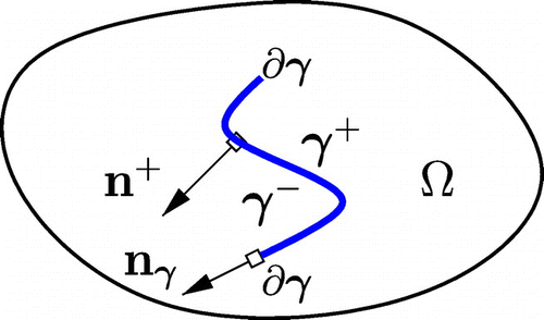
2.1. The model problem

Let the porous medium $\mathrm{\Omega }$ be a bounded domain in ${\mathbb{R}}^2$. We suppose that the fracture $\mathit{\gamma }\subset \mathrm{\Omega }$ is a regular, non-self-intersecting, curve of finite length and of bounded curvature. In this two-dimensional setting $\mathit{\partial }\mathit{\gamma }$, the boundary of $\mathit{\gamma }$, consists of the endpoints of $\mathit{\gamma }$ which we assume are distinct and do not lie on the boundary of $\mathrm{\Omega }$. Let ${\mathbf{n}}^{+}$ be a unit normal vector field on $\mathit{\gamma }$, and let ${\mathbf{n}}^{-}=-{\mathbf{n}}^{+}$. We distinguish the two sides of the fracture, ${\mathit{\gamma }}^{+}$ and ${\mathit{\gamma }}^{-}$, such that ${\mathbf{n}}^{+}$ (resp. ${\mathbf{n}}^{-}$) can be seen as the exterior normal to $\mathrm{\Omega }\backslash \mathit{\gamma }$ on ${\mathit{\gamma }}^{+}$ (resp. ${\mathit{\gamma }}^{-}$), see Figure 1. For a sufficiently regular function $\mathit{\phi }$ in $\mathrm{\Omega }\backslash \mathit{\gamma }$, we consider two traces ${\mathit{\phi }}^{+}$ and ${\mathit{\phi }}^{-}$ on $\mathit{\gamma }$, one for each side; see [15] for a more rigorous definition. We also introduce the tangential gradient ${\mathrm{\nabla }}_{\mathit{\tau }}$ and the tangential divergence ${\mathrm{div}}_{\mathit{\tau }}$ operators along the fracture.

The fracture interface model [14] may be written:(1) $$\begin{array}{c}\hfill \begin{array}{ccc}\hfill \mathbf{u}& =-\mathbf{K}\mathrm{\nabla }p& \text{in}\mathrm{\Omega }\backslash \mathit{\gamma },\hfill \\ \hfill \mathrm{div}\mathbf{u}& =f& \text{in}\mathrm{\Omega }\backslash \mathit{\gamma },\hfill \\ \hfill {\mathbf{u}}_{\mathit{\gamma }}& =-\mathit{\alpha }{\mathrm{\nabla }}_{\mathit{\tau }}{p}_{\mathit{\gamma }}& \text{in}\mathit{\gamma },\hfill \\ \hfill {\mathrm{div}}_{\mathit{\tau }}{\mathbf{u}}_{\mathit{\gamma }}& =f_{\mathit{\gamma }}+[[\mathbf{u}·\mathbf{n}]]& \text{in}\mathit{\gamma },\hfill \\ \hfill -\mathit{\beta }{\mathbf{u}}^{+}·{\mathbf{n}}^{+}+p^{+}& =p_{\mathit{\gamma }}& \text{on}{\mathit{\gamma }}^{+},\hfill \\ \hfill -\mathit{\beta }{\mathbf{u}}^{-}·{\mathbf{n}}^{-}+p^{-}& =p_{\mathit{\gamma }}& \text{on}{\mathit{\gamma }}^{-}.\hfill \end{array}\end{array}$$(1) (With respect to the model (4.1) in [14], the numerical parameter $\mathit{\xi }$ is taken equal to 1, since it has very little influence on the flow in most cases, see [14].)

The first two equations in (1(1) $$\begin{array}{c}\hfill \begin{array}{ccc}\hfill \mathbf{u}& =-\mathbf{K}\mathrm{\nabla }p& \text{in}\mathrm{\Omega }\backslash \mathit{\gamma },\hfill \\ \hfill \mathrm{div}\mathbf{u}& =f& \text{in}\mathrm{\Omega }\backslash \mathit{\gamma },\hfill \\ \hfill {\mathbf{u}}_{\mathit{\gamma }}& =-\mathit{\alpha }{\mathrm{\nabla }}_{\mathit{\tau }}{p}_{\mathit{\gamma }}& \text{in}\mathit{\gamma },\hfill \\ \hfill {\mathrm{div}}_{\mathit{\tau }}{\mathbf{u}}_{\mathit{\gamma }}& =f_{\mathit{\gamma }}+[[\mathbf{u}·\mathbf{n}]]& \text{in}\mathit{\gamma },\hfill \\ \hfill -\mathit{\beta }{\mathbf{u}}^{+}·{\mathbf{n}}^{+}+p^{+}& =p_{\mathit{\gamma }}& \text{on}{\mathit{\gamma }}^{+},\hfill \\ \hfill -\mathit{\beta }{\mathbf{u}}^{-}·{\mathbf{n}}^{-}+p^{-}& =p_{\mathit{\gamma }}& \text{on}{\mathit{\gamma }}^{-}.\hfill \end{array}\end{array}$$(1) ) are Darcy’s law and the law of mass conservation with a source term $f$ in the domain $\mathrm{\Omega }\backslash \mathit{\gamma }$. They relate the Darcy velocity $\mathbf{u}$ with the pressure p through the permeability tensor $\mathbf{K}$. The next equation is Darcy’s law, relating the tangential Darcy velocity ${\mathbf{u}}_{\mathit{\gamma }}$ to the fluid pressure in the fracture $p_{\mathit{\gamma }}$. The fourth equation is the law of mass conservation along the fracture $\mathit{\gamma }$, with a possible fracture source term $f_{\mathit{\gamma }}$, supplemented by an exchange term $[[\mathbf{u}·\mathbf{n}]]={\mathbf{u}}^{+}·{\mathbf{n}}^{+}+{\mathbf{u}}^{-}·{\mathbf{n}}^{-}$ accounting for fluid exchange between $\mathit{\gamma }$ and $\mathrm{\Omega }\backslash \mathit{\gamma }$. The last two equations that close the system represent an averaged Darcy law across normal cross sections of the physical fracture represented by $\mathit{\gamma }$.

The model (1(1) $$\begin{array}{c}\hfill \begin{array}{ccc}\hfill \mathbf{u}& =-\mathbf{K}\mathrm{\nabla }p& \text{in}\mathrm{\Omega }\backslash \mathit{\gamma },\hfill \\ \hfill \mathrm{div}\mathbf{u}& =f& \text{in}\mathrm{\Omega }\backslash \mathit{\gamma },\hfill \\ \hfill {\mathbf{u}}_{\mathit{\gamma }}& =-\mathit{\alpha }{\mathrm{\nabla }}_{\mathit{\tau }}{p}_{\mathit{\gamma }}& \text{in}\mathit{\gamma },\hfill \\ \hfill {\mathrm{div}}_{\mathit{\tau }}{\mathbf{u}}_{\mathit{\gamma }}& =f_{\mathit{\gamma }}+[[\mathbf{u}·\mathbf{n}]]& \text{in}\mathit{\gamma },\hfill \\ \hfill -\mathit{\beta }{\mathbf{u}}^{+}·{\mathbf{n}}^{+}+p^{+}& =p_{\mathit{\gamma }}& \text{on}{\mathit{\gamma }}^{+},\hfill \\ \hfill -\mathit{\beta }{\mathbf{u}}^{-}·{\mathbf{n}}^{-}+p^{-}& =p_{\mathit{\gamma }}& \text{on}{\mathit{\gamma }}^{-}.\hfill \end{array}\end{array}$$(1) ) is supplemented with the boundary conditions(2) $$\begin{array}{c}\hfill \begin{array}{cccc}\hfill p& =\overline{p}& \text{on}\mathit{\partial }\mathrm{\Omega },\hfill & \\ \hfill {\mathbf{u}}_{\mathit{\gamma }}·{\mathbf{n}}_{\mathit{\gamma }}& =0& \text{on}\mathit{\partial }\mathit{\gamma },\hfill \end{array}\end{array}$$(2)

where $\overline{p}$ is a given function, and ${\mathbf{n}}_{\mathit{\gamma }}$ is the unit normal vector field on $\mathit{\partial }\mathit{\gamma }$ pointing outwards from $\mathit{\gamma }$ (and tangent to $\mathit{\gamma }$ at its endpoints), see Figure 1. The condition ${\mathbf{u}}_{\mathit{\gamma }}·{\mathbf{n}}_{\mathit{\gamma }}=0$ is coherent with the hypothesis that the endpoints $\mathit{\partial }\mathit{\gamma }$ are inside the porous medium.

The coefficients $\mathit{\alpha }$ and $\mathit{\beta }$ are hydrogeological parameters characterizing the fracture: $\mathit{\alpha }$ represents an effective tangential permeability. In the case of (conducting) geological faults, $\mathit{\alpha }$ is positive and the Darcy velocity is generally discontinuous across the fracture ($[[\mathbf{u}·\mathbf{n}]]\ne 0$). In a two-dimension setting, $\mathit{\alpha }$ is the product of a thickness and a permeability divided by a length. The coefficient $\mathit{\beta }$ represents the inverse of an effective permeability normal to the fracture. So $\mathit{\beta }$ models the resistivity of the fracture to flow across it. In the case of geological barriers, $\mathit{\beta }$ is positive and the pressure is generally discontinuous across the fracture ($p^{+}\ne p^{-}$). In two dimensions, $\mathit{\beta }$ is the product of a thickness, a permeability and a length.

Our objective will be to determine both the location of the fracture $\mathit{\gamma }$ and the physical properties $\mathit{\alpha }$ and $\mathit{\beta }$ of the fracture.

We assume that the permeability tensor $\mathbf{K}$ is symmetric and positive definite, and bounded away from zero, and that the parameters $\mathit{\alpha }$ and $\mathit{\beta }$ satisfy the hypotheses(3) $$\begin{array}{c}\hfill \mathit{\alpha }\ge {\mathit{\alpha }}_{min}>0\text{and}\mathit{\beta }\ge 0.\end{array}$$(3)

Under these hypotheses, the model (1(1) $$\begin{array}{c}\hfill \begin{array}{ccc}\hfill \mathbf{u}& =-\mathbf{K}\mathrm{\nabla }p& \text{in}\mathrm{\Omega }\backslash \mathit{\gamma },\hfill \\ \hfill \mathrm{div}\mathbf{u}& =f& \text{in}\mathrm{\Omega }\backslash \mathit{\gamma },\hfill \\ \hfill {\mathbf{u}}_{\mathit{\gamma }}& =-\mathit{\alpha }{\mathrm{\nabla }}_{\mathit{\tau }}{p}_{\mathit{\gamma }}& \text{in}\mathit{\gamma },\hfill \\ \hfill {\mathrm{div}}_{\mathit{\tau }}{\mathbf{u}}_{\mathit{\gamma }}& =f_{\mathit{\gamma }}+[[\mathbf{u}·\mathbf{n}]]& \text{in}\mathit{\gamma },\hfill \\ \hfill -\mathit{\beta }{\mathbf{u}}^{+}·{\mathbf{n}}^{+}+p^{+}& =p_{\mathit{\gamma }}& \text{on}{\mathit{\gamma }}^{+},\hfill \\ \hfill -\mathit{\beta }{\mathbf{u}}^{-}·{\mathbf{n}}^{-}+p^{-}& =p_{\mathit{\gamma }}& \text{on}{\mathit{\gamma }}^{-}.\hfill \end{array}\end{array}$$(1) ) and (2(2) $$\begin{array}{c}\hfill \begin{array}{cccc}\hfill p& =\overline{p}& \text{on}\mathit{\partial }\mathrm{\Omega },\hfill & \\ \hfill {\mathbf{u}}_{\mathit{\gamma }}·{\mathbf{n}}_{\mathit{\gamma }}& =0& \text{on}\mathit{\partial }\mathit{\gamma },\hfill \end{array}\end{array}$$(2) ) is well-posed, see [14].

2.2. Discretization of the model problem

Let ${\mathcal{T}}_h$ be a finite element mesh of $\mathrm{\Omega }$, conforming with the fracture $\mathit{\gamma }$ in the sense that $\mathit{\gamma }$ is a subset of the union of the closures of the edges of the elements of ${\mathcal{T}}_h$. We denote by T, E, N, respectively, the elements (e.g. triangles), edges and nodes of ${\mathcal{T}}_h$, by ${\mathcal{E}}_T$ the boundary edges of an element T, by ${\mathcal{T}}_E$ the elements having E as an edge, by ${\mathcal{N}}_E$ the endpoints of an edge E, and by ${\mathcal{E}}_N$ the edges having N as an endpoint. Let ${\mathcal{E}}_h^i$ be the set of internal edges of ${\mathcal{T}}_h$ and ${\mathcal{E}}_h^e$ the set of boundary edges of ${\mathcal{T}}_h$, so that $\mathit{\partial }\mathrm{\Omega }={\bigcup }_{E\in {\mathcal{E}}_h^e}\overline{E}$ and ${\mathcal{E}}_h^e\cap {\mathcal{E}}_h^i=\mathrm{\varnothing }$. We denote by ${\mathcal{E}}_h\stackrel{\mathrm{def}}{=}{\mathcal{E}}_h^i\cup {\mathcal{E}}_h^e$ the set of all edges of ${\mathcal{T}}_h$.

We say that the fracture $\mathit{\gamma }$ is supported by the internal mesh edges to mean that $\mathit{\gamma }\subset {\bigcup }_{E\in {\mathcal{E}}_h^i}\overline{E}$, and we assume that the parameters $\mathit{\alpha }$ and $\mathit{\beta }$ are discretized by piecewise constant functions on these fracture edges. To simplify the search for independent faults and barriers, we discretize the fracture $\mathit{\gamma }$ as(4) $$\begin{array}{c}\hfill {\mathcal{F}}_h\stackrel{\mathrm{def}}{=}({\mathcal{F}}_{\mathit{\alpha }},{\mathcal{F}}_{\mathit{\beta }}),\end{array}$$(4)

where we have separated fault edges in ${\mathcal{F}}_{\mathit{\alpha }}$ from barrier edges in ${\mathcal{F}}_{\mathit{\beta }}$,(5) $$\begin{array}{c}\hfill {\mathcal{F}}_{\mathit{\alpha }}\stackrel{\mathrm{def}}{=}\{E\in {\mathcal{E}}_h^i|{\mathit{\alpha }}_E>0\}\text{and}{\mathcal{F}}_{\mathit{\beta }}\stackrel{\mathrm{def}}{=}\{E\in {\mathcal{E}}_h^i|{\mathit{\beta }}_E>0\}.\end{array}$$(5)

We denote the collections of fault (or tangential) and barrier (or normal) parameters by(6) $$\begin{array}{c}\hfill \mathit{\alpha }\stackrel{\mathrm{def}}{=}{({\mathit{\alpha }}_E)}_{E\in {\mathcal{F}}_{\mathit{\alpha }}}\text{and}\mathit{\beta }\stackrel{\mathrm{def}}{=}{({\mathit{\beta }}_E)}_{E\in {\mathcal{F}}_{\mathit{\beta }}}.\end{array}$$(6)

The sets of fault and barrier edges need not be disjoint. Let ${\mathcal{N}}_{\mathit{\alpha }}$ be the set of all nodes of ${\mathcal{F}}_{\mathit{\alpha }}$.

In order to simplify the presentation, we assume that the mesh is made up of square elements of size h, that the permeability tensor in $\mathrm{\Omega }$ is constant and scalar $\mathbf{K}=K\mathbf{I}$ (with $K>0$), and that the model (1(1) $$\begin{array}{c}\hfill \begin{array}{ccc}\hfill \mathbf{u}& =-\mathbf{K}\mathrm{\nabla }p& \text{in}\mathrm{\Omega }\backslash \mathit{\gamma },\hfill \\ \hfill \mathrm{div}\mathbf{u}& =f& \text{in}\mathrm{\Omega }\backslash \mathit{\gamma },\hfill \\ \hfill {\mathbf{u}}_{\mathit{\gamma }}& =-\mathit{\alpha }{\mathrm{\nabla }}_{\mathit{\tau }}{p}_{\mathit{\gamma }}& \text{in}\mathit{\gamma },\hfill \\ \hfill {\mathrm{div}}_{\mathit{\tau }}{\mathbf{u}}_{\mathit{\gamma }}& =f_{\mathit{\gamma }}+[[\mathbf{u}·\mathbf{n}]]& \text{in}\mathit{\gamma },\hfill \\ \hfill -\mathit{\beta }{\mathbf{u}}^{+}·{\mathbf{n}}^{+}+p^{+}& =p_{\mathit{\gamma }}& \text{on}{\mathit{\gamma }}^{+},\hfill \\ \hfill -\mathit{\beta }{\mathbf{u}}^{-}·{\mathbf{n}}^{-}+p^{-}& =p_{\mathit{\gamma }}& \text{on}{\mathit{\gamma }}^{-}.\hfill \end{array}\end{array}$$(1) ) and (2(2) $$\begin{array}{c}\hfill \begin{array}{cccc}\hfill p& =\overline{p}& \text{on}\mathit{\partial }\mathrm{\Omega },\hfill & \\ \hfill {\mathbf{u}}_{\mathit{\gamma }}·{\mathbf{n}}_{\mathit{\gamma }}& =0& \text{on}\mathit{\partial }\mathit{\gamma },\hfill \end{array}\end{array}$$(2) ) is discretized using a cell-centered finite volume method, see [25]. The discretization in the more general case of lowest order Raviart–Thomas mixed hybrid finite elements with general meshes is presented in [34]. These two discretizations in rectangular meshes are equivalent up to an approximate quadrature formula, see [35].

Let $P_T$, $P_E$ and $P_N$ be the pressure unknowns on an element $T\in {\mathcal{T}}_h$, an edge $E\in {\mathcal{E}}_h$ and a node $N\in {\mathcal{N}}_{\mathit{\alpha }}$. Let $U_{T,E}$ be the flow rate of fluid leaving an element $T\in {\mathcal{T}}_h$ through an edge $E\in {\mathcal{E}}_T$, let $U_{E,N}$ be the flow rate of fluid leaving an edge $E\in {\mathcal{F}}_{\mathit{\alpha }}$ through a node $N\in {\mathcal{N}}_E$. Using the notations $\mathit{\kappa }\stackrel{\mathrm{def}}{=}{K}^{-1}h$, $f_T\stackrel{\mathrm{def}}{=}{\int }_{T}f$, $f_E\stackrel{\mathrm{def}}{=}{\int }_E{f}_{\mathit{\gamma }}$, and ${\overline{P}}_E\stackrel{\mathrm{def}}{=}\frac{1}{|E|}{\int }_E\overline{p}$, the finite volume formulation of (1(1) $$\begin{array}{c}\hfill \begin{array}{ccc}\hfill \mathbf{u}& =-\mathbf{K}\mathrm{\nabla }p& \text{in}\mathrm{\Omega }\backslash \mathit{\gamma },\hfill \\ \hfill \mathrm{div}\mathbf{u}& =f& \text{in}\mathrm{\Omega }\backslash \mathit{\gamma },\hfill \\ \hfill {\mathbf{u}}_{\mathit{\gamma }}& =-\mathit{\alpha }{\mathrm{\nabla }}_{\mathit{\tau }}{p}_{\mathit{\gamma }}& \text{in}\mathit{\gamma },\hfill \\ \hfill {\mathrm{div}}_{\mathit{\tau }}{\mathbf{u}}_{\mathit{\gamma }}& =f_{\mathit{\gamma }}+[[\mathbf{u}·\mathbf{n}]]& \text{in}\mathit{\gamma },\hfill \\ \hfill -\mathit{\beta }{\mathbf{u}}^{+}·{\mathbf{n}}^{+}+p^{+}& =p_{\mathit{\gamma }}& \text{on}{\mathit{\gamma }}^{+},\hfill \\ \hfill -\mathit{\beta }{\mathbf{u}}^{-}·{\mathbf{n}}^{-}+p^{-}& =p_{\mathit{\gamma }}& \text{on}{\mathit{\gamma }}^{-}.\hfill \end{array}\end{array}$$(1) ) and (2(2) $$\begin{array}{c}\hfill \begin{array}{cccc}\hfill p& =\overline{p}& \text{on}\mathit{\partial }\mathrm{\Omega },\hfill & \\ \hfill {\mathbf{u}}_{\mathit{\gamma }}·{\mathbf{n}}_{\mathit{\gamma }}& =0& \text{on}\mathit{\partial }\mathit{\gamma },\hfill \end{array}\end{array}$$(2) ) reads(7) $$\begin{array}{c}\hfill \begin{array}{ccc}\hfill {\displaystyle {\sum }_{E\in {\mathcal{E}}_T}{U}_{T,E}}& =f_T,& \text{for all}T\in {\mathcal{T}}_h,\hfill \\ \hfill {\displaystyle \frac{\mathit{\kappa }}{2}{U}_{T,E}}& =P_T-P_E,& \text{for all}E\notin {\mathcal{F}}_{\mathit{\beta }},T\in {\mathcal{T}}_E,\hfill \\ \hfill {\displaystyle \left(\frac{\mathit{\kappa }}{2}+{\mathit{\beta }}_E\right)U_{T,E}}& =P_T-P_E,& \text{for all}E\in {\mathcal{F}}_{\mathit{\beta }},T\in {\mathcal{T}}_E,\hfill \\ \hfill {\displaystyle P_E}& ={\overline{P}}_E,& \text{for all}E\in {\mathcal{E}}_h^e,\hfill \\ \hfill {\displaystyle -{\sum }_{T\in {\mathcal{T}}_E}{U}_{T,E}}& =0,& \text{for all}E\notin {\mathcal{F}}_{\mathit{\alpha }},E\in {\mathcal{E}}_h^i,\hfill \end{array}\end{array}$$(7)

and(8) $$\begin{array}{c}\hfill \begin{array}{ccc}\hfill {\displaystyle -{\sum }_{T\in {\mathcal{T}}_E}{U}_{T,E}+{\sum }_{N\in {\mathcal{N}}_E}{U}_{E,N}}& =f_E,& \text{for all}E\in {\mathcal{F}}_{\mathit{\alpha }},\hfill \\ \hfill {\displaystyle \frac{h}{2{\mathit{\alpha }}_E}{U}_{E,N}}& =P_E-P_N,& \text{for all}E\in {\mathcal{F}}_{\mathit{\alpha }},N\in {\mathcal{N}}_E,\hfill \\ \hfill {\displaystyle {\sum }_{\begin{array}{c}E\in {\mathcal{F}}_{\mathit{\alpha }}\\ E\in {\mathcal{E}}_N\end{array}}{U}_{E,N}}& =0,& \text{for all}N\in {\mathcal{N}}_{\mathit{\alpha }},\hfill \end{array}\end{array}$$(8)

where the last equation already contains, for endpoints of the fault ${\mathcal{F}}_{\mathit{\alpha }}$, the no-flow condition ${\mathbf{u}}_{\mathit{\gamma }}·{\mathbf{n}}_{\mathit{\gamma }}=0$ of (2(2) $$\begin{array}{c}\hfill \begin{array}{cccc}\hfill p& =\overline{p}& \text{on}\mathit{\partial }\mathrm{\Omega },\hfill & \\ \hfill {\mathbf{u}}_{\mathit{\gamma }}·{\mathbf{n}}_{\mathit{\gamma }}& =0& \text{on}\mathit{\partial }\mathit{\gamma },\hfill \end{array}\end{array}$$(2) ).

In Section 4, the construction of fracture indicators will require to pass to the limit in the above equations when ${\mathit{\alpha }}_E\to 0$ on some edges of ${\mathcal{F}}_{\mathit{\alpha }}$. But a quick look at the second equation in (8(8) $$\begin{array}{c}\hfill \begin{array}{ccc}\hfill {\displaystyle -{\sum }_{T\in {\mathcal{T}}_E}{U}_{T,E}+{\sum }_{N\in {\mathcal{N}}_E}{U}_{E,N}}& =f_E,& \text{for all}E\in {\mathcal{F}}_{\mathit{\alpha }},\hfill \\ \hfill {\displaystyle \frac{h}{2{\mathit{\alpha }}_E}{U}_{E,N}}& =P_E-P_N,& \text{for all}E\in {\mathcal{F}}_{\mathit{\alpha }},N\in {\mathcal{N}}_E,\hfill \\ \hfill {\displaystyle {\sum }_{\begin{array}{c}E\in {\mathcal{F}}_{\mathit{\alpha }}\\ E\in {\mathcal{E}}_N\end{array}}{U}_{E,N}}& =0,& \text{for all}N\in {\mathcal{N}}_{\mathit{\alpha }},\hfill \end{array}\end{array}$$(8) ) let us foresee some problem in doing so. So we replace on all fault edges the flow rate unknown $U_{E,N}$ by a new unknown $V_{E,N}$ defined by (remember that ${\mathit{\alpha }}_E>0$ in this section)(9) $$\begin{array}{c}\hfill {\mathit{\alpha }}_E{V}_{E,N}=U_{E,N},\text{for all}E\in {\mathcal{F}}_{\mathit{\alpha }},N\in {\mathcal{N}}_E.\end{array}$$(9)

With these unknowns, (8(8) $$\begin{array}{c}\hfill \begin{array}{ccc}\hfill {\displaystyle -{\sum }_{T\in {\mathcal{T}}_E}{U}_{T,E}+{\sum }_{N\in {\mathcal{N}}_E}{U}_{E,N}}& =f_E,& \text{for all}E\in {\mathcal{F}}_{\mathit{\alpha }},\hfill \\ \hfill {\displaystyle \frac{h}{2{\mathit{\alpha }}_E}{U}_{E,N}}& =P_E-P_N,& \text{for all}E\in {\mathcal{F}}_{\mathit{\alpha }},N\in {\mathcal{N}}_E,\hfill \\ \hfill {\displaystyle {\sum }_{\begin{array}{c}E\in {\mathcal{F}}_{\mathit{\alpha }}\\ E\in {\mathcal{E}}_N\end{array}}{U}_{E,N}}& =0,& \text{for all}N\in {\mathcal{N}}_{\mathit{\alpha }},\hfill \end{array}\end{array}$$(8) ) is replaced by(10) $$\begin{array}{c}\hfill \begin{array}{ccc}\hfill {\displaystyle -{\sum }_{T\in {\mathcal{T}}_E}{U}_{T,E}+{\mathit{\alpha }}_E{\sum }_{N\in {\mathcal{N}}_E}{V}_{E,N}}& =f_E,& \text{for all}E\in {\mathcal{F}}_{\mathit{\alpha }},\hfill \\ \hfill {\displaystyle \frac{h}{2}{V}_{E,N}}& =P_E-P_N,& \text{for all}E\in {\mathcal{F}}_{\mathit{\alpha }},N\in {\mathcal{N}}_E,\hfill \\ \hfill {\displaystyle {\sum }_{\begin{array}{c}E\in {\mathcal{F}}_{\mathit{\alpha }}\\ E\in {\mathcal{E}}_N\end{array}}{\mathit{\alpha }}_E{V}_{E,N}}& =0,& \text{for all}N\in {\mathcal{N}}_{\mathit{\alpha }}.\hfill \end{array}\end{array}$$(10)

The second equation in (10(10) $$\begin{array}{c}\hfill \begin{array}{ccc}\hfill {\displaystyle -{\sum }_{T\in {\mathcal{T}}_E}{U}_{T,E}+{\mathit{\alpha }}_E{\sum }_{N\in {\mathcal{N}}_E}{V}_{E,N}}& =f_E,& \text{for all}E\in {\mathcal{F}}_{\mathit{\alpha }},\hfill \\ \hfill {\displaystyle \frac{h}{2}{V}_{E,N}}& =P_E-P_N,& \text{for all}E\in {\mathcal{F}}_{\mathit{\alpha }},N\in {\mathcal{N}}_E,\hfill \\ \hfill {\displaystyle {\sum }_{\begin{array}{c}E\in {\mathcal{F}}_{\mathit{\alpha }}\\ E\in {\mathcal{E}}_N\end{array}}{\mathit{\alpha }}_E{V}_{E,N}}& =0,& \text{for all}N\in {\mathcal{N}}_{\mathit{\alpha }}.\hfill \end{array}\end{array}$$(10) ) shows that the new unknown $V_{E,N}$ is the (discrete) pressure gradient between the middle of edge E and its end node N.

For the sake of simplicity, we suppose, in the sequel, the fracture source term to be zero ($f_E=0$ in (10(10) $$\begin{array}{c}\hfill \begin{array}{ccc}\hfill {\displaystyle -{\sum }_{T\in {\mathcal{T}}_E}{U}_{T,E}+{\mathit{\alpha }}_E{\sum }_{N\in {\mathcal{N}}_E}{V}_{E,N}}& =f_E,& \text{for all}E\in {\mathcal{F}}_{\mathit{\alpha }},\hfill \\ \hfill {\displaystyle \frac{h}{2}{V}_{E,N}}& =P_E-P_N,& \text{for all}E\in {\mathcal{F}}_{\mathit{\alpha }},N\in {\mathcal{N}}_E,\hfill \\ \hfill {\displaystyle {\sum }_{\begin{array}{c}E\in {\mathcal{F}}_{\mathit{\alpha }}\\ E\in {\mathcal{E}}_N\end{array}}{\mathit{\alpha }}_E{V}_{E,N}}& =0,& \text{for all}N\in {\mathcal{N}}_{\mathit{\alpha }}.\hfill \end{array}\end{array}$$(10) )). To sum up, the (discrete) direct model for the simulation of flow in a porous domain $\mathrm{\Omega }$ containing a discrete fracture $({\mathcal{F}}_{\mathit{\alpha }},{\mathcal{F}}_{\mathit{\beta }})$ with fault and barrier parameters $(\mathit{\alpha },\mathit{\beta })$ is made up of equations (7(7) $$\begin{array}{c}\hfill \begin{array}{ccc}\hfill {\displaystyle {\sum }_{E\in {\mathcal{E}}_T}{U}_{T,E}}& =f_T,& \text{for all}T\in {\mathcal{T}}_h,\hfill \\ \hfill {\displaystyle \frac{\mathit{\kappa }}{2}{U}_{T,E}}& =P_T-P_E,& \text{for all}E\notin {\mathcal{F}}_{\mathit{\beta }},T\in {\mathcal{T}}_E,\hfill \\ \hfill {\displaystyle \left(\frac{\mathit{\kappa }}{2}+{\mathit{\beta }}_E\right)U_{T,E}}& =P_T-P_E,& \text{for all}E\in {\mathcal{F}}_{\mathit{\beta }},T\in {\mathcal{T}}_E,\hfill \\ \hfill {\displaystyle P_E}& ={\overline{P}}_E,& \text{for all}E\in {\mathcal{E}}_h^e,\hfill \\ \hfill {\displaystyle -{\sum }_{T\in {\mathcal{T}}_E}{U}_{T,E}}& =0,& \text{for all}E\notin {\mathcal{F}}_{\mathit{\alpha }},E\in {\mathcal{E}}_h^i,\hfill \end{array}\end{array}$$(7) ) and (10(10) $$\begin{array}{c}\hfill \begin{array}{ccc}\hfill {\displaystyle -{\sum }_{T\in {\mathcal{T}}_E}{U}_{T,E}+{\mathit{\alpha }}_E{\sum }_{N\in {\mathcal{N}}_E}{V}_{E,N}}& =f_E,& \text{for all}E\in {\mathcal{F}}_{\mathit{\alpha }},\hfill \\ \hfill {\displaystyle \frac{h}{2}{V}_{E,N}}& =P_E-P_N,& \text{for all}E\in {\mathcal{F}}_{\mathit{\alpha }},N\in {\mathcal{N}}_E,\hfill \\ \hfill {\displaystyle {\sum }_{\begin{array}{c}E\in {\mathcal{F}}_{\mathit{\alpha }}\\ E\in {\mathcal{E}}_N\end{array}}{\mathit{\alpha }}_E{V}_{E,N}}& =0,& \text{for all}N\in {\mathcal{N}}_{\mathit{\alpha }}.\hfill \end{array}\end{array}$$(10) ). Thus the direct problem associates to the fracture, i.e. the pair ${\mathcal{F}}_h=({\mathcal{F}}_{\mathit{\alpha }},{\mathcal{F}}_{\mathit{\beta }})$ together with the fracture parameters, the solution of the direct model.

3. The inverse problem

Focusing now on the inverse problem, we assume that pressure and/or flow measurements are available at some points of the domain $\mathrm{\Omega }$, and consider the problem of estimating the location and parameters of the corresponding fracture. For the sake of simplicity, we limit ourselves in this section to the simple case where a pressure measurement ${\overline{P}}_T$ is available for each element T in ${\mathcal{T}}_h$. More realistic measurements will be considered for numerical experiments in Section 6.

3.1. The least-squares formulation

In the framework of an iterative process for solving the inverse problem, let the current fracture be described by its edges ${\mathcal{F}}_h=({\mathcal{F}}_{\mathit{\alpha }},{\mathcal{F}}_{\mathit{\beta }})$ and parameters $(\mathit{\alpha },\mathit{\beta })$. We associate the current fracture with the least-square data misfit(11) $$\begin{array}{c}\hfill {\mathcal{J}}_{{\mathcal{F}}_h}(\mathit{\alpha },\mathit{\beta })\stackrel{\mathrm{def}}{=}\frac{1}{2}\sum _{T\in {\mathcal{T}}_h}{(P_T-{\overline{P}}_T)}^2,\end{array}$$(11)

where $P_T$ is given by the current model (7(7) $$\begin{array}{c}\hfill \begin{array}{ccc}\hfill {\displaystyle {\sum }_{E\in {\mathcal{E}}_T}{U}_{T,E}}& =f_T,& \text{for all}T\in {\mathcal{T}}_h,\hfill \\ \hfill {\displaystyle \frac{\mathit{\kappa }}{2}{U}_{T,E}}& =P_T-P_E,& \text{for all}E\notin {\mathcal{F}}_{\mathit{\beta }},T\in {\mathcal{T}}_E,\hfill \\ \hfill {\displaystyle \left(\frac{\mathit{\kappa }}{2}+{\mathit{\beta }}_E\right)U_{T,E}}& =P_T-P_E,& \text{for all}E\in {\mathcal{F}}_{\mathit{\beta }},T\in {\mathcal{T}}_E,\hfill \\ \hfill {\displaystyle P_E}& ={\overline{P}}_E,& \text{for all}E\in {\mathcal{E}}_h^e,\hfill \\ \hfill {\displaystyle -{\sum }_{T\in {\mathcal{T}}_E}{U}_{T,E}}& =0,& \text{for all}E\notin {\mathcal{F}}_{\mathit{\alpha }},E\in {\mathcal{E}}_h^i,\hfill \end{array}\end{array}$$(7) ) and (10(10) $$\begin{array}{c}\hfill \begin{array}{ccc}\hfill {\displaystyle -{\sum }_{T\in {\mathcal{T}}_E}{U}_{T,E}+{\mathit{\alpha }}_E{\sum }_{N\in {\mathcal{N}}_E}{V}_{E,N}}& =f_E,& \text{for all}E\in {\mathcal{F}}_{\mathit{\alpha }},\hfill \\ \hfill {\displaystyle \frac{h}{2}{V}_{E,N}}& =P_E-P_N,& \text{for all}E\in {\mathcal{F}}_{\mathit{\alpha }},N\in {\mathcal{N}}_E,\hfill \\ \hfill {\displaystyle {\sum }_{\begin{array}{c}E\in {\mathcal{F}}_{\mathit{\alpha }}\\ E\in {\mathcal{E}}_N\end{array}}{\mathit{\alpha }}_E{V}_{E,N}}& =0,& \text{for all}N\in {\mathcal{N}}_{\mathit{\alpha }}.\hfill \end{array}\end{array}$$(10) ) set on the current fracture ${\mathcal{F}}_h$.

If this misfit is above the uncertainty level of the data measurements, one is led to consider adding new candidate edges $\mathrm{\Delta }{\mathcal{F}}_h=(\mathrm{\Delta }{\mathcal{F}}_{\mathit{\alpha }},\mathrm{\Delta }{\mathcal{F}}_{\mathit{\beta }})$ to the current fracture ${\mathcal{F}}_h$. We suppose that current and candidate fractures have no common edge,(12) $$\begin{array}{c}\hfill {\mathcal{F}}_{\mathit{\alpha }}\cap \mathrm{\Delta }{\mathcal{F}}_{\mathit{\alpha }}=\mathrm{\varnothing }\text{and}{\mathcal{F}}_{\mathit{\beta }}\cap \mathrm{\Delta }{\mathcal{F}}_{\mathit{\beta }}=\mathrm{\varnothing }.\end{array}$$(12)

Let $\mathrm{\Delta }{\mathcal{N}}_{\mathit{\alpha }}$ be the set of new nodes of the candidate fault $\mathrm{\Delta }{\mathcal{F}}_{\mathit{\alpha }}$, so that(13) $$\begin{array}{c}\hfill {\mathcal{N}}_{\mathit{\alpha }}\cap \mathrm{\Delta }{\mathcal{N}}_{\mathit{\alpha }}=\mathrm{\varnothing }.\end{array}$$(13)

We use nominal parameters $\overline{\mathit{\alpha }}$ and $\overline{\mathit{\beta }}$ to describe typical parameter profiles expected along the new candidate fault and barrier edges. In the absence of such information, nominal parameters are chosen to be constant. We model the introduction of the candidate fracture by new intensity parameters ${\mathit{\epsilon }}_{\mathit{\alpha }}$ and ${\mathit{\epsilon }}_{\mathit{\beta }}$, which let the fracture parameters $\mathit{\alpha }$ and $\mathit{\beta }$ grow from zero to their nominal value and beyond,(14) $$\begin{array}{cc}\hfill {\mathit{\alpha }}_E={\mathit{\epsilon }}_{\mathit{\alpha }}{\overline{\mathit{\alpha }}}_E,& \text{for all}E\in \mathrm{\Delta }{\mathcal{F}}_{\mathit{\alpha }},{\mathit{\epsilon }}_{\mathit{\alpha }}\ge 0,\hfill \end{array}$$(14) (15) $$\begin{array}{cc}\hfill {\mathit{\beta }}_E={\mathit{\epsilon }}_{\mathit{\beta }}{\overline{\mathit{\beta }}}_E,& \text{for all}E\in \mathrm{\Delta }{\mathcal{F}}_{\mathit{\beta }},{\mathit{\epsilon }}_{\mathit{\beta }}\ge 0.\hfill \end{array}$$(15)

Because of (14(14) $$\begin{array}{cc}\hfill {\mathit{\alpha }}_E={\mathit{\epsilon }}_{\mathit{\alpha }}{\overline{\mathit{\alpha }}}_E,& \text{for all}E\in \mathrm{\Delta }{\mathcal{F}}_{\mathit{\alpha }},{\mathit{\epsilon }}_{\mathit{\alpha }}\ge 0,\hfill \end{array}$$(14) ), the last equation of (10(10) $$\begin{array}{c}\hfill \begin{array}{ccc}\hfill {\displaystyle -{\sum }_{T\in {\mathcal{T}}_E}{U}_{T,E}+{\mathit{\alpha }}_E{\sum }_{N\in {\mathcal{N}}_E}{V}_{E,N}}& =f_E,& \text{for all}E\in {\mathcal{F}}_{\mathit{\alpha }},\hfill \\ \hfill {\displaystyle \frac{h}{2}{V}_{E,N}}& =P_E-P_N,& \text{for all}E\in {\mathcal{F}}_{\mathit{\alpha }},N\in {\mathcal{N}}_E,\hfill \\ \hfill {\displaystyle {\sum }_{\begin{array}{c}E\in {\mathcal{F}}_{\mathit{\alpha }}\\ E\in {\mathcal{E}}_N\end{array}}{\mathit{\alpha }}_E{V}_{E,N}}& =0,& \text{for all}N\in {\mathcal{N}}_{\mathit{\alpha }}.\hfill \end{array}\end{array}$$(10) ) can be divided by ${\mathit{\epsilon }}_{\mathit{\alpha }}$ on $\mathrm{\Delta }{\mathcal{N}}_{\mathit{\alpha }}$, thus the model (7(7) $$\begin{array}{c}\hfill \begin{array}{ccc}\hfill {\displaystyle {\sum }_{E\in {\mathcal{E}}_T}{U}_{T,E}}& =f_T,& \text{for all}T\in {\mathcal{T}}_h,\hfill \\ \hfill {\displaystyle \frac{\mathit{\kappa }}{2}{U}_{T,E}}& =P_T-P_E,& \text{for all}E\notin {\mathcal{F}}_{\mathit{\beta }},T\in {\mathcal{T}}_E,\hfill \\ \hfill {\displaystyle \left(\frac{\mathit{\kappa }}{2}+{\mathit{\beta }}_E\right)U_{T,E}}& =P_T-P_E,& \text{for all}E\in {\mathcal{F}}_{\mathit{\beta }},T\in {\mathcal{T}}_E,\hfill \\ \hfill {\displaystyle P_E}& ={\overline{P}}_E,& \text{for all}E\in {\mathcal{E}}_h^e,\hfill \\ \hfill {\displaystyle -{\sum }_{T\in {\mathcal{T}}_E}{U}_{T,E}}& =0,& \text{for all}E\notin {\mathcal{F}}_{\mathit{\alpha }},E\in {\mathcal{E}}_h^i,\hfill \end{array}\end{array}$$(7) ) and (10(10) $$\begin{array}{c}\hfill \begin{array}{ccc}\hfill {\displaystyle -{\sum }_{T\in {\mathcal{T}}_E}{U}_{T,E}+{\mathit{\alpha }}_E{\sum }_{N\in {\mathcal{N}}_E}{V}_{E,N}}& =f_E,& \text{for all}E\in {\mathcal{F}}_{\mathit{\alpha }},\hfill \\ \hfill {\displaystyle \frac{h}{2}{V}_{E,N}}& =P_E-P_N,& \text{for all}E\in {\mathcal{F}}_{\mathit{\alpha }},N\in {\mathcal{N}}_E,\hfill \\ \hfill {\displaystyle {\sum }_{\begin{array}{c}E\in {\mathcal{F}}_{\mathit{\alpha }}\\ E\in {\mathcal{E}}_N\end{array}}{\mathit{\alpha }}_E{V}_{E,N}}& =0,& \text{for all}N\in {\mathcal{N}}_{\mathit{\alpha }}.\hfill \end{array}\end{array}$$(10) ) set on both current and candidate fractures ${\mathcal{F}}_h$ and $\mathrm{\Delta }{\mathcal{F}}_h$ simplifies to the tentative model (16) $$\begin{array}{c}\hfill \begin{array}{ccc}\hfill {\displaystyle {\sum }_{E\in {\mathcal{E}}_T}{U}_{T,E}}& =f_T,& \text{for all}T\in {\mathcal{T}}_h,\hfill \\ \hfill {\displaystyle \frac{\mathit{\kappa }}{2}{U}_{T,E}}& =P_T-P_E,& \text{for all}E\notin {\mathcal{F}}_{\mathit{\beta }}\cup \mathrm{\Delta }{\mathcal{F}}_{\mathit{\beta }},T\in {\mathcal{T}}_E,\hfill \\ \hfill {\displaystyle \left(\frac{\mathit{\kappa }}{2}+{\mathit{\beta }}_E\right)U_{T,E}}& =P_T-P_E,& \text{for all}E\in {\mathcal{F}}_{\mathit{\beta }}\cup \mathrm{\Delta }{\mathcal{F}}_{\mathit{\beta }},T\in {\mathcal{T}}_E,\hfill \\ \hfill {\displaystyle P_E}& ={\overline{P}}_E,& \text{for all}E\in {\mathcal{E}}_h^e,\hfill \\ \hfill {\displaystyle -{\sum }_{T\in {\mathcal{T}}_E}{U}_{T,E}}& =0,& \text{for all}E\notin {\mathcal{F}}_{\mathit{\alpha }}\cup \mathrm{\Delta }{\mathcal{F}}_{\mathit{\alpha }},E\in {\mathcal{E}}_h^i,\hfill \\ \hfill {\displaystyle -{\sum }_{T\in {\mathcal{T}}_E}{U}_{T,E}+{\mathit{\alpha }}_E{\sum }_{N\in {\mathcal{N}}_E}{V}_{E,N}}& =0,& \text{for all}E\in {\mathcal{F}}_{\mathit{\alpha }}\cup \mathrm{\Delta }{\mathcal{F}}_{\mathit{\alpha }},\hfill \\ \hfill {\displaystyle \frac{h}{2}{V}_{E,N}}& =P_E-P_N,& \text{for all}E\in {\mathcal{F}}_{\mathit{\alpha }}\cup \mathrm{\Delta }{\mathcal{F}}_{\mathit{\alpha }},N\in {\mathcal{N}}_E,\hfill \\ \hfill {\displaystyle {\sum }_{\begin{array}{c}E\in {\mathcal{F}}_{\mathit{\alpha }}\cup \mathrm{\Delta }{\mathcal{F}}_{\mathit{\alpha }}\\ E\in {\mathcal{E}}_N\end{array}}{\mathit{\alpha }}_E{V}_{E,N}}& =0,& \text{for all}N\in {\mathcal{N}}_{\mathit{\alpha }},\hfill \\ \hfill {\displaystyle {\sum }_{\begin{array}{c}E\in \mathrm{\Delta }{\mathcal{F}}_{\mathit{\alpha }}\\ E\in {\mathcal{E}}_N\end{array}}{\overline{\mathit{\alpha }}}_E{V}_{E,N}}& =0,& \text{for all}N\in \mathrm{\Delta }{\mathcal{N}}_{\mathit{\alpha }}.\hfill \end{array}\end{array}$$(16)

When ${\mathit{\epsilon }}_{\mathit{\alpha }}={\mathit{\epsilon }}_{\mathit{\beta }}=0$, one easily checks that the tentative model (16(16) $$\begin{array}{c}\hfill \begin{array}{ccc}\hfill {\displaystyle {\sum }_{E\in {\mathcal{E}}_T}{U}_{T,E}}& =f_T,& \text{for all}T\in {\mathcal{T}}_h,\hfill \\ \hfill {\displaystyle \frac{\mathit{\kappa }}{2}{U}_{T,E}}& =P_T-P_E,& \text{for all}E\notin {\mathcal{F}}_{\mathit{\beta }}\cup \mathrm{\Delta }{\mathcal{F}}_{\mathit{\beta }},T\in {\mathcal{T}}_E,\hfill \\ \hfill {\displaystyle \left(\frac{\mathit{\kappa }}{2}+{\mathit{\beta }}_E\right)U_{T,E}}& =P_T-P_E,& \text{for all}E\in {\mathcal{F}}_{\mathit{\beta }}\cup \mathrm{\Delta }{\mathcal{F}}_{\mathit{\beta }},T\in {\mathcal{T}}_E,\hfill \\ \hfill {\displaystyle P_E}& ={\overline{P}}_E,& \text{for all}E\in {\mathcal{E}}_h^e,\hfill \\ \hfill {\displaystyle -{\sum }_{T\in {\mathcal{T}}_E}{U}_{T,E}}& =0,& \text{for all}E\notin {\mathcal{F}}_{\mathit{\alpha }}\cup \mathrm{\Delta }{\mathcal{F}}_{\mathit{\alpha }},E\in {\mathcal{E}}_h^i,\hfill \\ \hfill {\displaystyle -{\sum }_{T\in {\mathcal{T}}_E}{U}_{T,E}+{\mathit{\alpha }}_E{\sum }_{N\in {\mathcal{N}}_E}{V}_{E,N}}& =0,& \text{for all}E\in {\mathcal{F}}_{\mathit{\alpha }}\cup \mathrm{\Delta }{\mathcal{F}}_{\mathit{\alpha }},\hfill \\ \hfill {\displaystyle \frac{h}{2}{V}_{E,N}}& =P_E-P_N,& \text{for all}E\in {\mathcal{F}}_{\mathit{\alpha }}\cup \mathrm{\Delta }{\mathcal{F}}_{\mathit{\alpha }},N\in {\mathcal{N}}_E,\hfill \\ \hfill {\displaystyle {\sum }_{\begin{array}{c}E\in {\mathcal{F}}_{\mathit{\alpha }}\cup \mathrm{\Delta }{\mathcal{F}}_{\mathit{\alpha }}\\ E\in {\mathcal{E}}_N\end{array}}{\mathit{\alpha }}_E{V}_{E,N}}& =0,& \text{for all}N\in {\mathcal{N}}_{\mathit{\alpha }},\hfill \\ \hfill {\displaystyle {\sum }_{\begin{array}{c}E\in \mathrm{\Delta }{\mathcal{F}}_{\mathit{\alpha }}\\ E\in {\mathcal{E}}_N\end{array}}{\overline{\mathit{\alpha }}}_E{V}_{E,N}}& =0,& \text{for all}N\in \mathrm{\Delta }{\mathcal{N}}_{\mathit{\alpha }}.\hfill \end{array}\end{array}$$(16) ) reduces to the current model (7(7) $$\begin{array}{c}\hfill \begin{array}{ccc}\hfill {\displaystyle {\sum }_{E\in {\mathcal{E}}_T}{U}_{T,E}}& =f_T,& \text{for all}T\in {\mathcal{T}}_h,\hfill \\ \hfill {\displaystyle \frac{\mathit{\kappa }}{2}{U}_{T,E}}& =P_T-P_E,& \text{for all}E\notin {\mathcal{F}}_{\mathit{\beta }},T\in {\mathcal{T}}_E,\hfill \\ \hfill {\displaystyle \left(\frac{\mathit{\kappa }}{2}+{\mathit{\beta }}_E\right)U_{T,E}}& =P_T-P_E,& \text{for all}E\in {\mathcal{F}}_{\mathit{\beta }},T\in {\mathcal{T}}_E,\hfill \\ \hfill {\displaystyle P_E}& ={\overline{P}}_E,& \text{for all}E\in {\mathcal{E}}_h^e,\hfill \\ \hfill {\displaystyle -{\sum }_{T\in {\mathcal{T}}_E}{U}_{T,E}}& =0,& \text{for all}E\notin {\mathcal{F}}_{\mathit{\alpha }},E\in {\mathcal{E}}_h^i,\hfill \end{array}\end{array}$$(7) ) and (10(10) $$\begin{array}{c}\hfill \begin{array}{ccc}\hfill {\displaystyle -{\sum }_{T\in {\mathcal{T}}_E}{U}_{T,E}+{\mathit{\alpha }}_E{\sum }_{N\in {\mathcal{N}}_E}{V}_{E,N}}& =f_E,& \text{for all}E\in {\mathcal{F}}_{\mathit{\alpha }},\hfill \\ \hfill {\displaystyle \frac{h}{2}{V}_{E,N}}& =P_E-P_N,& \text{for all}E\in {\mathcal{F}}_{\mathit{\alpha }},N\in {\mathcal{N}}_E,\hfill \\ \hfill {\displaystyle {\sum }_{\begin{array}{c}E\in {\mathcal{F}}_{\mathit{\alpha }}\\ E\in {\mathcal{E}}_N\end{array}}{\mathit{\alpha }}_E{V}_{E,N}}& =0,& \text{for all}N\in {\mathcal{N}}_{\mathit{\alpha }}.\hfill \end{array}\end{array}$$(10) ) complemented with the limit fault model set on the candidate fault,(17) $$\begin{array}{c}\hfill \begin{array}{ccc}\hfill {\displaystyle \frac{h}{2}{V}_{E,N}}& =P_E-P_N& \text{for all}E\in \mathrm{\Delta }{\mathcal{F}}_{\mathit{\alpha }},N\in {\mathcal{N}}_E,\hfill \\ \hfill {\displaystyle {\sum }_{\begin{array}{c}E\in \mathrm{\Delta }{\mathcal{F}}_{\mathit{\alpha }}\\ E\in {\mathcal{E}}_N\end{array}}{\overline{\mathit{\alpha }}}_E{V}_{E,N}}& =0& \text{for all}N\in \mathrm{\Delta }{\mathcal{N}}_{\mathit{\alpha }}.\hfill \end{array}\end{array}$$(17)

Hence, we see that, for any ${\mathit{\epsilon }}_{\mathit{\alpha }},{\mathit{\epsilon }}_{\mathit{\beta }}\ge 0$, the tentative model (16(16) $$\begin{array}{c}\hfill \begin{array}{ccc}\hfill {\displaystyle {\sum }_{E\in {\mathcal{E}}_T}{U}_{T,E}}& =f_T,& \text{for all}T\in {\mathcal{T}}_h,\hfill \\ \hfill {\displaystyle \frac{\mathit{\kappa }}{2}{U}_{T,E}}& =P_T-P_E,& \text{for all}E\notin {\mathcal{F}}_{\mathit{\beta }}\cup \mathrm{\Delta }{\mathcal{F}}_{\mathit{\beta }},T\in {\mathcal{T}}_E,\hfill \\ \hfill {\displaystyle \left(\frac{\mathit{\kappa }}{2}+{\mathit{\beta }}_E\right)U_{T,E}}& =P_T-P_E,& \text{for all}E\in {\mathcal{F}}_{\mathit{\beta }}\cup \mathrm{\Delta }{\mathcal{F}}_{\mathit{\beta }},T\in {\mathcal{T}}_E,\hfill \\ \hfill {\displaystyle P_E}& ={\overline{P}}_E,& \text{for all}E\in {\mathcal{E}}_h^e,\hfill \\ \hfill {\displaystyle -{\sum }_{T\in {\mathcal{T}}_E}{U}_{T,E}}& =0,& \text{for all}E\notin {\mathcal{F}}_{\mathit{\alpha }}\cup \mathrm{\Delta }{\mathcal{F}}_{\mathit{\alpha }},E\in {\mathcal{E}}_h^i,\hfill \\ \hfill {\displaystyle -{\sum }_{T\in {\mathcal{T}}_E}{U}_{T,E}+{\mathit{\alpha }}_E{\sum }_{N\in {\mathcal{N}}_E}{V}_{E,N}}& =0,& \text{for all}E\in {\mathcal{F}}_{\mathit{\alpha }}\cup \mathrm{\Delta }{\mathcal{F}}_{\mathit{\alpha }},\hfill \\ \hfill {\displaystyle \frac{h}{2}{V}_{E,N}}& =P_E-P_N,& \text{for all}E\in {\mathcal{F}}_{\mathit{\alpha }}\cup \mathrm{\Delta }{\mathcal{F}}_{\mathit{\alpha }},N\in {\mathcal{N}}_E,\hfill \\ \hfill {\displaystyle {\sum }_{\begin{array}{c}E\in {\mathcal{F}}_{\mathit{\alpha }}\cup \mathrm{\Delta }{\mathcal{F}}_{\mathit{\alpha }}\\ E\in {\mathcal{E}}_N\end{array}}{\mathit{\alpha }}_E{V}_{E,N}}& =0,& \text{for all}N\in {\mathcal{N}}_{\mathit{\alpha }},\hfill \\ \hfill {\displaystyle {\sum }_{\begin{array}{c}E\in \mathrm{\Delta }{\mathcal{F}}_{\mathit{\alpha }}\\ E\in {\mathcal{E}}_N\end{array}}{\overline{\mathit{\alpha }}}_E{V}_{E,N}}& =0,& \text{for all}N\in \mathrm{\Delta }{\mathcal{N}}_{\mathit{\alpha }}.\hfill \end{array}\end{array}$$(16) ) determines uniquely $P_T$, $P_E$, and $U_{T,E}$ on all elements and edges, and $P_N$ and $V_{E,N}$ on all nodes and edges of the current and candidate faults. So, we can extend the definition (11(11) $$\begin{array}{c}\hfill {\mathcal{J}}_{{\mathcal{F}}_h}(\mathit{\alpha },\mathit{\beta })\stackrel{\mathrm{def}}{=}\frac{1}{2}\sum _{T\in {\mathcal{T}}_h}{(P_T-{\overline{P}}_T)}^2,\end{array}$$(11) ) of the least-squares data misfit to a function of the intensity parameters ${\mathit{\epsilon }}_{\mathit{\alpha }},{\mathit{\epsilon }}_{\mathit{\beta }}\ge 0$ on the candidate fracture by(18) $$\begin{array}{c}\hfill {\mathcal{J}}_{\mathrm{\Delta }{\mathcal{F}}_h}({\mathit{\epsilon }}_{\mathit{\alpha }},{\mathit{\epsilon }}_{\mathit{\beta }})\stackrel{\mathrm{def}}{=}\frac{1}{2}\sum _{T\in {\mathcal{T}}_h}{(P_T-{\overline{P}}_T)}^2,\end{array}$$(18)

where $P_T$ is now given by the tentative model (14(14) $$\begin{array}{cc}\hfill {\mathit{\alpha }}_E={\mathit{\epsilon }}_{\mathit{\alpha }}{\overline{\mathit{\alpha }}}_E,& \text{for all}E\in \mathrm{\Delta }{\mathcal{F}}_{\mathit{\alpha }},{\mathit{\epsilon }}_{\mathit{\alpha }}\ge 0,\hfill \end{array}$$(14) )–(16(16) $$\begin{array}{c}\hfill \begin{array}{ccc}\hfill {\displaystyle {\sum }_{E\in {\mathcal{E}}_T}{U}_{T,E}}& =f_T,& \text{for all}T\in {\mathcal{T}}_h,\hfill \\ \hfill {\displaystyle \frac{\mathit{\kappa }}{2}{U}_{T,E}}& =P_T-P_E,& \text{for all}E\notin {\mathcal{F}}_{\mathit{\beta }}\cup \mathrm{\Delta }{\mathcal{F}}_{\mathit{\beta }},T\in {\mathcal{T}}_E,\hfill \\ \hfill {\displaystyle \left(\frac{\mathit{\kappa }}{2}+{\mathit{\beta }}_E\right)U_{T,E}}& =P_T-P_E,& \text{for all}E\in {\mathcal{F}}_{\mathit{\beta }}\cup \mathrm{\Delta }{\mathcal{F}}_{\mathit{\beta }},T\in {\mathcal{T}}_E,\hfill \\ \hfill {\displaystyle P_E}& ={\overline{P}}_E,& \text{for all}E\in {\mathcal{E}}_h^e,\hfill \\ \hfill {\displaystyle -{\sum }_{T\in {\mathcal{T}}_E}{U}_{T,E}}& =0,& \text{for all}E\notin {\mathcal{F}}_{\mathit{\alpha }}\cup \mathrm{\Delta }{\mathcal{F}}_{\mathit{\alpha }},E\in {\mathcal{E}}_h^i,\hfill \\ \hfill {\displaystyle -{\sum }_{T\in {\mathcal{T}}_E}{U}_{T,E}+{\mathit{\alpha }}_E{\sum }_{N\in {\mathcal{N}}_E}{V}_{E,N}}& =0,& \text{for all}E\in {\mathcal{F}}_{\mathit{\alpha }}\cup \mathrm{\Delta }{\mathcal{F}}_{\mathit{\alpha }},\hfill \\ \hfill {\displaystyle \frac{h}{2}{V}_{E,N}}& =P_E-P_N,& \text{for all}E\in {\mathcal{F}}_{\mathit{\alpha }}\cup \mathrm{\Delta }{\mathcal{F}}_{\mathit{\alpha }},N\in {\mathcal{N}}_E,\hfill \\ \hfill {\displaystyle {\sum }_{\begin{array}{c}E\in {\mathcal{F}}_{\mathit{\alpha }}\cup \mathrm{\Delta }{\mathcal{F}}_{\mathit{\alpha }}\\ E\in {\mathcal{E}}_N\end{array}}{\mathit{\alpha }}_E{V}_{E,N}}& =0,& \text{for all}N\in {\mathcal{N}}_{\mathit{\alpha }},\hfill \\ \hfill {\displaystyle {\sum }_{\begin{array}{c}E\in \mathrm{\Delta }{\mathcal{F}}_{\mathit{\alpha }}\\ E\in {\mathcal{E}}_N\end{array}}{\overline{\mathit{\alpha }}}_E{V}_{E,N}}& =0,& \text{for all}N\in \mathrm{\Delta }{\mathcal{N}}_{\mathit{\alpha }}.\hfill \end{array}\end{array}$$(16) ). The purpose of the indicator algorithm developed in the next sections will be to select, in a computationally efficient way, the candidate fractures $\mathrm{\Delta }{\mathcal{F}}_h$ for which there exists ${\mathit{\epsilon }}_{\mathit{\alpha }},{\mathit{\epsilon }}_{\mathit{\beta }}>0$ such that(19) $$\begin{array}{c}\hfill {\mathcal{J}}_{\mathrm{\Delta }{\mathcal{F}}_h}({\mathit{\epsilon }}_{\mathit{\alpha }},{\mathit{\epsilon }}_{\mathit{\beta }})<{\mathcal{J}}_{\mathrm{\Delta }{\mathcal{F}}_h}(0,0)={\mathcal{J}}_{{\mathcal{F}}_h}(\mathit{\alpha },\mathit{\beta }),\end{array}$$(19)

with a preferably large decrease of the data misfit.

Remark 3.1:

Replacing the hypothesis ${\mathit{\epsilon }}_{\mathit{\alpha }}={\mathit{\epsilon }}_{\mathit{\beta }}=0$ in (14(14) $$\begin{array}{cc}\hfill {\mathit{\alpha }}_E={\mathit{\epsilon }}_{\mathit{\alpha }}{\overline{\mathit{\alpha }}}_E,& \text{for all}E\in \mathrm{\Delta }{\mathcal{F}}_{\mathit{\alpha }},{\mathit{\epsilon }}_{\mathit{\alpha }}\ge 0,\hfill \end{array}$$(14) ) and (15(15) $$\begin{array}{cc}\hfill {\mathit{\beta }}_E={\mathit{\epsilon }}_{\mathit{\beta }}{\overline{\mathit{\beta }}}_E,& \text{for all}E\in \mathrm{\Delta }{\mathcal{F}}_{\mathit{\beta }},{\mathit{\epsilon }}_{\mathit{\beta }}\ge 0.\hfill \end{array}$$(15) ) by the weaker assumption that $\mathit{\alpha },\mathit{\beta }\to 0$ for all candidate edges of $\mathrm{\Delta }{\mathcal{F}}_h$, makes the last equation in (10(10) $$\begin{array}{c}\hfill \begin{array}{ccc}\hfill {\displaystyle -{\sum }_{T\in {\mathcal{T}}_E}{U}_{T,E}+{\mathit{\alpha }}_E{\sum }_{N\in {\mathcal{N}}_E}{V}_{E,N}}& =f_E,& \text{for all}E\in {\mathcal{F}}_{\mathit{\alpha }},\hfill \\ \hfill {\displaystyle \frac{h}{2}{V}_{E,N}}& =P_E-P_N,& \text{for all}E\in {\mathcal{F}}_{\mathit{\alpha }},N\in {\mathcal{N}}_E,\hfill \\ \hfill {\displaystyle {\sum }_{\begin{array}{c}E\in {\mathcal{F}}_{\mathit{\alpha }}\\ E\in {\mathcal{E}}_N\end{array}}{\mathit{\alpha }}_E{V}_{E,N}}& =0,& \text{for all}N\in {\mathcal{N}}_{\mathit{\alpha }}.\hfill \end{array}\end{array}$$(10) ) disappear on nodes of $\mathrm{\Delta }{\mathcal{N}}_{\mathit{\alpha }}$: unknowns ${(P_N)}_{N\in \mathrm{\Delta }{\mathcal{N}}_{\mathit{\alpha }}}$ and ${(V_{E,N})}_{E\in \mathrm{\Delta }{\mathcal{F}}_{\mathit{\alpha }},N\in {\mathcal{N}}_E}$ become undetermined for the limit equations, but all other unknowns remain uniquely determined.

Actually, in Section 4, the key ingredient for the definition of fracture indicators is the fading of fracture parameters on the candidate fracture. And, choosing a specific direction in the space of fracture edge parameters through (14(14) $$\begin{array}{cc}\hfill {\mathit{\alpha }}_E={\mathit{\epsilon }}_{\mathit{\alpha }}{\overline{\mathit{\alpha }}}_E,& \text{for all}E\in \mathrm{\Delta }{\mathcal{F}}_{\mathit{\alpha }},{\mathit{\epsilon }}_{\mathit{\alpha }}\ge 0,\hfill \end{array}$$(14) ) and (15(15) $$\begin{array}{cc}\hfill {\mathit{\beta }}_E={\mathit{\epsilon }}_{\mathit{\beta }}{\overline{\mathit{\beta }}}_E,& \text{for all}E\in \mathrm{\Delta }{\mathcal{F}}_{\mathit{\beta }},{\mathit{\epsilon }}_{\mathit{\beta }}\ge 0.\hfill \end{array}$$(15) ), makes the solution of the tentative model (16(16) $$\begin{array}{c}\hfill \begin{array}{ccc}\hfill {\displaystyle {\sum }_{E\in {\mathcal{E}}_T}{U}_{T,E}}& =f_T,& \text{for all}T\in {\mathcal{T}}_h,\hfill \\ \hfill {\displaystyle \frac{\mathit{\kappa }}{2}{U}_{T,E}}& =P_T-P_E,& \text{for all}E\notin {\mathcal{F}}_{\mathit{\beta }}\cup \mathrm{\Delta }{\mathcal{F}}_{\mathit{\beta }},T\in {\mathcal{T}}_E,\hfill \\ \hfill {\displaystyle \left(\frac{\mathit{\kappa }}{2}+{\mathit{\beta }}_E\right)U_{T,E}}& =P_T-P_E,& \text{for all}E\in {\mathcal{F}}_{\mathit{\beta }}\cup \mathrm{\Delta }{\mathcal{F}}_{\mathit{\beta }},T\in {\mathcal{T}}_E,\hfill \\ \hfill {\displaystyle P_E}& ={\overline{P}}_E,& \text{for all}E\in {\mathcal{E}}_h^e,\hfill \\ \hfill {\displaystyle -{\sum }_{T\in {\mathcal{T}}_E}{U}_{T,E}}& =0,& \text{for all}E\notin {\mathcal{F}}_{\mathit{\alpha }}\cup \mathrm{\Delta }{\mathcal{F}}_{\mathit{\alpha }},E\in {\mathcal{E}}_h^i,\hfill \\ \hfill {\displaystyle -{\sum }_{T\in {\mathcal{T}}_E}{U}_{T,E}+{\mathit{\alpha }}_E{\sum }_{N\in {\mathcal{N}}_E}{V}_{E,N}}& =0,& \text{for all}E\in {\mathcal{F}}_{\mathit{\alpha }}\cup \mathrm{\Delta }{\mathcal{F}}_{\mathit{\alpha }},\hfill \\ \hfill {\displaystyle \frac{h}{2}{V}_{E,N}}& =P_E-P_N,& \text{for all}E\in {\mathcal{F}}_{\mathit{\alpha }}\cup \mathrm{\Delta }{\mathcal{F}}_{\mathit{\alpha }},N\in {\mathcal{N}}_E,\hfill \\ \hfill {\displaystyle {\sum }_{\begin{array}{c}E\in {\mathcal{F}}_{\mathit{\alpha }}\cup \mathrm{\Delta }{\mathcal{F}}_{\mathit{\alpha }}\\ E\in {\mathcal{E}}_N\end{array}}{\mathit{\alpha }}_E{V}_{E,N}}& =0,& \text{for all}N\in {\mathcal{N}}_{\mathit{\alpha }},\hfill \\ \hfill {\displaystyle {\sum }_{\begin{array}{c}E\in \mathrm{\Delta }{\mathcal{F}}_{\mathit{\alpha }}\\ E\in {\mathcal{E}}_N\end{array}}{\overline{\mathit{\alpha }}}_E{V}_{E,N}}& =0,& \text{for all}N\in \mathrm{\Delta }{\mathcal{N}}_{\mathit{\alpha }}.\hfill \end{array}\end{array}$$(16) ) behave continuously for vanishing intensity parameters.

3.2. Gradient with respect to the intensity parameters

We compute now the gradient of the objective function with respect to ${\mathit{\epsilon }}_{\mathit{\alpha }}$ and ${\mathit{\epsilon }}_{\mathit{\beta }}$ by the adjoint state method, for instance see [30, Section 2.4]. For the sake of simplicity, the Dirichlet boundary condition (fourth equation in (16(16) $$\begin{array}{c}\hfill \begin{array}{ccc}\hfill {\displaystyle {\sum }_{E\in {\mathcal{E}}_T}{U}_{T,E}}& =f_T,& \text{for all}T\in {\mathcal{T}}_h,\hfill \\ \hfill {\displaystyle \frac{\mathit{\kappa }}{2}{U}_{T,E}}& =P_T-P_E,& \text{for all}E\notin {\mathcal{F}}_{\mathit{\beta }}\cup \mathrm{\Delta }{\mathcal{F}}_{\mathit{\beta }},T\in {\mathcal{T}}_E,\hfill \\ \hfill {\displaystyle \left(\frac{\mathit{\kappa }}{2}+{\mathit{\beta }}_E\right)U_{T,E}}& =P_T-P_E,& \text{for all}E\in {\mathcal{F}}_{\mathit{\beta }}\cup \mathrm{\Delta }{\mathcal{F}}_{\mathit{\beta }},T\in {\mathcal{T}}_E,\hfill \\ \hfill {\displaystyle P_E}& ={\overline{P}}_E,& \text{for all}E\in {\mathcal{E}}_h^e,\hfill \\ \hfill {\displaystyle -{\sum }_{T\in {\mathcal{T}}_E}{U}_{T,E}}& =0,& \text{for all}E\notin {\mathcal{F}}_{\mathit{\alpha }}\cup \mathrm{\Delta }{\mathcal{F}}_{\mathit{\alpha }},E\in {\mathcal{E}}_h^i,\hfill \\ \hfill {\displaystyle -{\sum }_{T\in {\mathcal{T}}_E}{U}_{T,E}+{\mathit{\alpha }}_E{\sum }_{N\in {\mathcal{N}}_E}{V}_{E,N}}& =0,& \text{for all}E\in {\mathcal{F}}_{\mathit{\alpha }}\cup \mathrm{\Delta }{\mathcal{F}}_{\mathit{\alpha }},\hfill \\ \hfill {\displaystyle \frac{h}{2}{V}_{E,N}}& =P_E-P_N,& \text{for all}E\in {\mathcal{F}}_{\mathit{\alpha }}\cup \mathrm{\Delta }{\mathcal{F}}_{\mathit{\alpha }},N\in {\mathcal{N}}_E,\hfill \\ \hfill {\displaystyle {\sum }_{\begin{array}{c}E\in {\mathcal{F}}_{\mathit{\alpha }}\cup \mathrm{\Delta }{\mathcal{F}}_{\mathit{\alpha }}\\ E\in {\mathcal{E}}_N\end{array}}{\mathit{\alpha }}_E{V}_{E,N}}& =0,& \text{for all}N\in {\mathcal{N}}_{\mathit{\alpha }},\hfill \\ \hfill {\displaystyle {\sum }_{\begin{array}{c}E\in \mathrm{\Delta }{\mathcal{F}}_{\mathit{\alpha }}\\ E\in {\mathcal{E}}_N\end{array}}{\overline{\mathit{\alpha }}}_E{V}_{E,N}}& =0,& \text{for all}N\in \mathrm{\Delta }{\mathcal{N}}_{\mathit{\alpha }}.\hfill \end{array}\end{array}$$(16) )) is not written explicitly, it is understood that whenever E is a boundary edge, $P_E$ means ${\overline{P}}_E$ (and hence its differential vanishes). With this convention, the vector of edge pressure unknowns becomes ${(P_E)}_{E\in {\mathcal{E}}_h^i}$.

The Lagrangian associated with the minimization of the objective function (18(18) $$\begin{array}{c}\hfill {\mathcal{J}}_{\mathrm{\Delta }{\mathcal{F}}_h}({\mathit{\epsilon }}_{\mathit{\alpha }},{\mathit{\epsilon }}_{\mathit{\beta }})\stackrel{\mathrm{def}}{=}\frac{1}{2}\sum _{T\in {\mathcal{T}}_h}{(P_T-{\overline{P}}_T)}^2,\end{array}$$(18) ) under the constraint of the state equations (16(16) $$\begin{array}{c}\hfill \begin{array}{ccc}\hfill {\displaystyle {\sum }_{E\in {\mathcal{E}}_T}{U}_{T,E}}& =f_T,& \text{for all}T\in {\mathcal{T}}_h,\hfill \\ \hfill {\displaystyle \frac{\mathit{\kappa }}{2}{U}_{T,E}}& =P_T-P_E,& \text{for all}E\notin {\mathcal{F}}_{\mathit{\beta }}\cup \mathrm{\Delta }{\mathcal{F}}_{\mathit{\beta }},T\in {\mathcal{T}}_E,\hfill \\ \hfill {\displaystyle \left(\frac{\mathit{\kappa }}{2}+{\mathit{\beta }}_E\right)U_{T,E}}& =P_T-P_E,& \text{for all}E\in {\mathcal{F}}_{\mathit{\beta }}\cup \mathrm{\Delta }{\mathcal{F}}_{\mathit{\beta }},T\in {\mathcal{T}}_E,\hfill \\ \hfill {\displaystyle P_E}& ={\overline{P}}_E,& \text{for all}E\in {\mathcal{E}}_h^e,\hfill \\ \hfill {\displaystyle -{\sum }_{T\in {\mathcal{T}}_E}{U}_{T,E}}& =0,& \text{for all}E\notin {\mathcal{F}}_{\mathit{\alpha }}\cup \mathrm{\Delta }{\mathcal{F}}_{\mathit{\alpha }},E\in {\mathcal{E}}_h^i,\hfill \\ \hfill {\displaystyle -{\sum }_{T\in {\mathcal{T}}_E}{U}_{T,E}+{\mathit{\alpha }}_E{\sum }_{N\in {\mathcal{N}}_E}{V}_{E,N}}& =0,& \text{for all}E\in {\mathcal{F}}_{\mathit{\alpha }}\cup \mathrm{\Delta }{\mathcal{F}}_{\mathit{\alpha }},\hfill \\ \hfill {\displaystyle \frac{h}{2}{V}_{E,N}}& =P_E-P_N,& \text{for all}E\in {\mathcal{F}}_{\mathit{\alpha }}\cup \mathrm{\Delta }{\mathcal{F}}_{\mathit{\alpha }},N\in {\mathcal{N}}_E,\hfill \\ \hfill {\displaystyle {\sum }_{\begin{array}{c}E\in {\mathcal{F}}_{\mathit{\alpha }}\cup \mathrm{\Delta }{\mathcal{F}}_{\mathit{\alpha }}\\ E\in {\mathcal{E}}_N\end{array}}{\mathit{\alpha }}_E{V}_{E,N}}& =0,& \text{for all}N\in {\mathcal{N}}_{\mathit{\alpha }},\hfill \\ \hfill {\displaystyle {\sum }_{\begin{array}{c}E\in \mathrm{\Delta }{\mathcal{F}}_{\mathit{\alpha }}\\ E\in {\mathcal{E}}_N\end{array}}{\overline{\mathit{\alpha }}}_E{V}_{E,N}}& =0,& \text{for all}N\in \mathrm{\Delta }{\mathcal{N}}_{\mathit{\alpha }}.\hfill \end{array}\end{array}$$(16) ) for the current and candidate fractures ${\mathcal{F}}_h\cup \mathrm{\Delta }{\mathcal{F}}_h$ is then(20) $$\begin{array}{ccc}\hfill \mathcal{L}(X,\mathrm{\Lambda };{\mathit{\epsilon }}_{\mathit{\alpha }},{\mathit{\epsilon }}_{\mathit{\beta }})& \stackrel{\mathrm{def}}{=}\hfill & \hfill \frac{1}{2}\sum _{T\in {\mathcal{T}}_h}{(P_T-{\overline{P}}_T)}^2\\ \hfill & +\sum _{T\in {\mathcal{T}}_h}\left(-\sum _{E\in {\mathcal{E}}_T}{U}_{T,E}+f_T\right){\mathit{\lambda }}_T\hfill \\ \hfill & +\sum _{E\notin {\mathcal{F}}_{\mathit{\beta }}\cup \mathrm{\Delta }{\mathcal{F}}_{\mathit{\beta }}}\sum _{T\in {\mathcal{T}}_E}\left(\frac{\mathit{\kappa }}{2}{U}_{T,E}-P_T+P_E\right){\mathit{\mu }}_{T,E}\hfill \\ \hfill & +\sum _{E\in {\mathcal{F}}_{\mathit{\beta }}\cup \mathrm{\Delta }{\mathcal{F}}_{\mathit{\beta }}}\sum _{T\in {\mathcal{T}}_E}\left(\left(\frac{\mathit{\kappa }}{2}+{\mathit{\beta }}_E\right)U_{T,E}-P_T+P_E\right){\mathit{\mu }}_{T,E}\hfill \\ \hfill & +\sum _{\begin{array}{c}E\notin {\mathcal{F}}_{\mathit{\alpha }}\cup \mathrm{\Delta }{\mathcal{F}}_{\mathit{\alpha }}\\ E\in {\mathcal{E}}_h^i\end{array}}\sum _{T\in {\mathcal{T}}_E}{U}_{T,E}{\mathit{\lambda }}_E\hfill \\ \hfill & +\sum _{E\in {\mathcal{F}}_{\mathit{\alpha }}\cup \mathrm{\Delta }{\mathcal{F}}_{\mathit{\alpha }}}\left(\sum _{T\in {\mathcal{T}}_E}{U}_{T,E}-{\mathit{\alpha }}_E\sum _{N\in {\mathcal{N}}_E}{V}_{E,N}\right){\mathit{\lambda }}_E\hfill \\ \hfill & +\sum _{E\in {\mathcal{F}}_{\mathit{\alpha }}\cup \mathrm{\Delta }{\mathcal{F}}_{\mathit{\alpha }}}\sum _{N\in {\mathcal{N}}_E}\left(\frac{h}{2}{V}_{E,N}-P_E+P_N\right){\mathit{\mu }}_{E,N}\hfill \\ \hfill & +\sum _{N\in {\mathcal{N}}_{\mathit{\alpha }}}\sum _{\begin{array}{c}E\in {\mathcal{F}}_{\mathit{\alpha }}\cup \mathrm{\Delta }{\mathcal{F}}_{\mathit{\alpha }}\\ E\in {\mathcal{E}}_N\end{array}}{\mathit{\alpha }}_E{V}_{E,N}{\mathit{\lambda }}_N\hfill \\ \hfill & +\sum _{N\in \mathrm{\Delta }{\mathcal{N}}_{\mathit{\alpha }}}\sum _{\begin{array}{c}E\in \mathrm{\Delta }{\mathcal{F}}_{\mathit{\alpha }}\\ E\in {\mathcal{E}}_N\end{array}}{\overline{\mathit{\alpha }}}_E{V}_{E,N}{\overline{\mathit{\lambda }}}_N,\hfill \end{array}$$(20)

where ${\mathit{\epsilon }}_{\mathit{\alpha }}$ and ${\mathit{\epsilon }}_{\mathit{\beta }}$ are the intensity parameters, $X\stackrel{\mathrm{def}}{=}(P_t,P_e,P_n,U_{te},V_{en})$ is the state vector, and $\mathrm{\Lambda }\stackrel{\mathrm{def}}{=}({\mathit{\lambda }}_t,{\mathit{\lambda }}_e,{\mathit{\lambda }}_n,{\overline{\mathit{\lambda }}}_n,{\mathit{\mu }}_{te},{\mathit{\mu }}_{en})$ is the adjoint state vector, with the notations(21) $$\begin{array}{cc}& P_t\stackrel{\mathrm{def}}{=}{(P_T)}_{T\in {\mathcal{T}}_h},U_{te}\stackrel{\mathrm{def}}{=}{(U_{T,E})}_{T\in {\mathcal{T}}_h,E\in {\mathcal{E}}_T},\hfill \\ \hfill & P_e\stackrel{\mathrm{def}}{=}{(P_E)}_{E\in {\mathcal{E}}_h^i},V_{en}\stackrel{\mathrm{def}}{=}{(V_{E,N})}_{E\in {\mathcal{F}}_{\mathit{\alpha }}\cup \mathrm{\Delta }{\mathcal{F}}_{\mathit{\alpha }},N\in {\mathcal{N}}_E},\hfill \\ \hfill & P_n\stackrel{\mathrm{def}}{=}{(P_N)}_{N\in {\mathcal{N}}_{\mathit{\alpha }}\cup \mathrm{\Delta }{\mathcal{N}}_{\mathit{\alpha }}},\hfill \\ \hfill & {\mathit{\lambda }}_t\stackrel{\mathrm{def}}{=}{({\mathit{\lambda }}_T)}_{T\in {\mathcal{T}}_h},{\mathit{\mu }}_{te}\stackrel{\mathrm{def}}{=}{({\mathit{\mu }}_{T,E})}_{T\in {\mathcal{T}}_h,E\in {\mathcal{E}}_T},\hfill \\ \hfill & {\mathit{\lambda }}_e\stackrel{\mathrm{def}}{=}{({\mathit{\lambda }}_E)}_{E\in {\mathcal{E}}_h^i},{\mathit{\mu }}_{en}\stackrel{\mathrm{def}}{=}{({\mathit{\mu }}_{E,N})}_{E\in {\mathcal{F}}_{\mathit{\alpha }}\cup \mathrm{\Delta }{\mathcal{F}}_{\mathit{\alpha }},N\in {\mathcal{N}}_E},\hfill \\ \hfill & {\mathit{\lambda }}_n\stackrel{\mathrm{def}}{=}{({\mathit{\lambda }}_N)}_{N\in {\mathcal{N}}_{\mathit{\alpha }}},{\overline{\mathit{\lambda }}}_n\stackrel{\mathrm{def}}{=}{({\overline{\mathit{\lambda }}}_N)}_{N\in \mathrm{\Delta }{\mathcal{N}}_{\mathit{\alpha }}}.\hfill \end{array}$$(21)

Let $X({\mathit{\epsilon }}_{\mathit{\alpha }},{\mathit{\epsilon }}_{\mathit{\beta }})$ denote the state vector corresponding to the solution of the tentative model (16(16) $$\begin{array}{c}\hfill \begin{array}{ccc}\hfill {\displaystyle {\sum }_{E\in {\mathcal{E}}_T}{U}_{T,E}}& =f_T,& \text{for all}T\in {\mathcal{T}}_h,\hfill \\ \hfill {\displaystyle \frac{\mathit{\kappa }}{2}{U}_{T,E}}& =P_T-P_E,& \text{for all}E\notin {\mathcal{F}}_{\mathit{\beta }}\cup \mathrm{\Delta }{\mathcal{F}}_{\mathit{\beta }},T\in {\mathcal{T}}_E,\hfill \\ \hfill {\displaystyle \left(\frac{\mathit{\kappa }}{2}+{\mathit{\beta }}_E\right)U_{T,E}}& =P_T-P_E,& \text{for all}E\in {\mathcal{F}}_{\mathit{\beta }}\cup \mathrm{\Delta }{\mathcal{F}}_{\mathit{\beta }},T\in {\mathcal{T}}_E,\hfill \\ \hfill {\displaystyle P_E}& ={\overline{P}}_E,& \text{for all}E\in {\mathcal{E}}_h^e,\hfill \\ \hfill {\displaystyle -{\sum }_{T\in {\mathcal{T}}_E}{U}_{T,E}}& =0,& \text{for all}E\notin {\mathcal{F}}_{\mathit{\alpha }}\cup \mathrm{\Delta }{\mathcal{F}}_{\mathit{\alpha }},E\in {\mathcal{E}}_h^i,\hfill \\ \hfill {\displaystyle -{\sum }_{T\in {\mathcal{T}}_E}{U}_{T,E}+{\mathit{\alpha }}_E{\sum }_{N\in {\mathcal{N}}_E}{V}_{E,N}}& =0,& \text{for all}E\in {\mathcal{F}}_{\mathit{\alpha }}\cup \mathrm{\Delta }{\mathcal{F}}_{\mathit{\alpha }},\hfill \\ \hfill {\displaystyle \frac{h}{2}{V}_{E,N}}& =P_E-P_N,& \text{for all}E\in {\mathcal{F}}_{\mathit{\alpha }}\cup \mathrm{\Delta }{\mathcal{F}}_{\mathit{\alpha }},N\in {\mathcal{N}}_E,\hfill \\ \hfill {\displaystyle {\sum }_{\begin{array}{c}E\in {\mathcal{F}}_{\mathit{\alpha }}\cup \mathrm{\Delta }{\mathcal{F}}_{\mathit{\alpha }}\\ E\in {\mathcal{E}}_N\end{array}}{\mathit{\alpha }}_E{V}_{E,N}}& =0,& \text{for all}N\in {\mathcal{N}}_{\mathit{\alpha }},\hfill \\ \hfill {\displaystyle {\sum }_{\begin{array}{c}E\in \mathrm{\Delta }{\mathcal{F}}_{\mathit{\alpha }}\\ E\in {\mathcal{E}}_N\end{array}}{\overline{\mathit{\alpha }}}_E{V}_{E,N}}& =0,& \text{for all}N\in \mathrm{\Delta }{\mathcal{N}}_{\mathit{\alpha }}.\hfill \end{array}\end{array}$$(16) ) with the fracture parameters $\mathit{\alpha }$ and $\mathit{\beta }$ defined by (14(14) $$\begin{array}{cc}\hfill {\mathit{\alpha }}_E={\mathit{\epsilon }}_{\mathit{\alpha }}{\overline{\mathit{\alpha }}}_E,& \text{for all}E\in \mathrm{\Delta }{\mathcal{F}}_{\mathit{\alpha }},{\mathit{\epsilon }}_{\mathit{\alpha }}\ge 0,\hfill \end{array}$$(14) ) and (15(15) $$\begin{array}{cc}\hfill {\mathit{\beta }}_E={\mathit{\epsilon }}_{\mathit{\beta }}{\overline{\mathit{\beta }}}_E,& \text{for all}E\in \mathrm{\Delta }{\mathcal{F}}_{\mathit{\beta }},{\mathit{\epsilon }}_{\mathit{\beta }}\ge 0.\hfill \end{array}$$(15) ) on the candidate fracture $\mathrm{\Delta }{\mathcal{F}}_{\mathit{\alpha }}$. Let $\mathrm{\Lambda }$ be a given adjoint state vector. Then, for all ${\mathit{\epsilon }}_{\mathit{\alpha }},{\mathit{\epsilon }}_{\mathit{\beta }}\ge 0$, we have the identity(22) $$\begin{array}{c}\hfill {\mathcal{J}}_{\mathrm{\Delta }{\mathcal{F}}_h}({\mathit{\epsilon }}_{\mathit{\alpha }},{\mathit{\epsilon }}_{\mathit{\beta }})=\mathcal{L}(X({\mathit{\epsilon }}_{\mathit{\alpha }},{\mathit{\epsilon }}_{\mathit{\beta }}),\mathrm{\Lambda };{\mathit{\epsilon }}_{\mathit{\alpha }},{\mathit{\epsilon }}_{\mathit{\beta }}).\end{array}$$(22)

Differentiation with respect to parameters ${\mathit{\epsilon }}_{\mathit{\alpha }}$ and ${\mathit{\epsilon }}_{\mathit{\beta }}$ gives (remember that $\mathrm{\Lambda }$ is given)(23) $$\begin{array}{c}\hfill \mathit{\delta }{\mathcal{J}}_{\mathrm{\Delta }{\mathcal{F}}_h}({\mathit{\epsilon }}_{\mathit{\alpha }},{\mathit{\epsilon }}_{\mathit{\beta }})=\mathit{\delta }\mathcal{L}(X({\mathit{\epsilon }}_{\mathit{\alpha }},{\mathit{\epsilon }}_{\mathit{\beta }}),\mathrm{\Lambda };{\mathit{\epsilon }}_{\mathit{\alpha }},{\mathit{\epsilon }}_{\mathit{\beta }}),\end{array}$$(23)

hence, for all ${\mathit{\epsilon }}_{\mathit{\alpha }},{\mathit{\epsilon }}_{\mathit{\beta }}\ge 0$,(24) $$\begin{array}{c}\hfill \mathit{\delta }{\mathcal{J}}_{\mathrm{\Delta }{\mathcal{F}}_h}({\mathit{\epsilon }}_{\mathit{\alpha }},{\mathit{\epsilon }}_{\mathit{\beta }})=\frac{\mathit{\partial }\mathcal{L}}{\mathit{\partial }X}(X({\mathit{\epsilon }}_{\mathit{\alpha }},{\mathit{\epsilon }}_{\mathit{\beta }}),\mathrm{\Lambda };{\mathit{\epsilon }}_{\mathit{\alpha }},{\mathit{\epsilon }}_{\mathit{\beta }})\mathit{\delta }X+\frac{\mathit{\partial }\mathcal{L}}{\mathit{\partial }({\mathit{\epsilon }}_{\mathit{\alpha }},{\mathit{\epsilon }}_{\mathit{\beta }})}(X({\mathit{\epsilon }}_{\mathit{\alpha }},{\mathit{\epsilon }}_{\mathit{\beta }}),\mathrm{\Lambda };{\mathit{\epsilon }}_{\mathit{\alpha }},{\mathit{\epsilon }}_{\mathit{\beta }})\mathit{\delta }({\mathit{\epsilon }}_{\mathit{\alpha }},{\mathit{\epsilon }}_{\mathit{\beta }}).\end{array}$$(24)

This identity holds for any adjoint state vector $\mathrm{\Lambda }$. Thus, nothing can prevent us from choosing for $\mathrm{\Lambda }$ precisely the unique solution $\mathrm{\Lambda }({\mathit{\epsilon }}_{\mathit{\alpha }},{\mathit{\epsilon }}_{\mathit{\beta }})$ of the adjoint equations such that(25) $$\begin{array}{c}\hfill \frac{\mathit{\partial }\mathcal{L}}{\mathit{\partial }X}(X({\mathit{\epsilon }}_{\mathit{\alpha }},{\mathit{\epsilon }}_{\mathit{\beta }}),\mathrm{\Lambda };{\mathit{\epsilon }}_{\mathit{\alpha }},{\mathit{\epsilon }}_{\mathit{\beta }})\mathit{\delta }X=0,\forall \mathit{\delta }X.\end{array}$$(25)

Then, (24(24) $$\begin{array}{c}\hfill \mathit{\delta }{\mathcal{J}}_{\mathrm{\Delta }{\mathcal{F}}_h}({\mathit{\epsilon }}_{\mathit{\alpha }},{\mathit{\epsilon }}_{\mathit{\beta }})=\frac{\mathit{\partial }\mathcal{L}}{\mathit{\partial }X}(X({\mathit{\epsilon }}_{\mathit{\alpha }},{\mathit{\epsilon }}_{\mathit{\beta }}),\mathrm{\Lambda };{\mathit{\epsilon }}_{\mathit{\alpha }},{\mathit{\epsilon }}_{\mathit{\beta }})\mathit{\delta }X+\frac{\mathit{\partial }\mathcal{L}}{\mathit{\partial }({\mathit{\epsilon }}_{\mathit{\alpha }},{\mathit{\epsilon }}_{\mathit{\beta }})}(X({\mathit{\epsilon }}_{\mathit{\alpha }},{\mathit{\epsilon }}_{\mathit{\beta }}),\mathrm{\Lambda };{\mathit{\epsilon }}_{\mathit{\alpha }},{\mathit{\epsilon }}_{\mathit{\beta }})\mathit{\delta }({\mathit{\epsilon }}_{\mathit{\alpha }},{\mathit{\epsilon }}_{\mathit{\beta }}).\end{array}$$(24) ) simplifies to the desired gradient equations, for all ${\mathit{\epsilon }}_{\mathit{\alpha }},{\mathit{\epsilon }}_{\mathit{\beta }}\ge 0$,(26) $$\begin{array}{c}\hfill \mathit{\delta }{\mathcal{J}}_{\mathrm{\Delta }{\mathcal{F}}_h}({\mathit{\epsilon }}_{\mathit{\alpha }},{\mathit{\epsilon }}_{\mathit{\beta }})=\frac{\mathit{\partial }\mathcal{L}}{\mathit{\partial }({\mathit{\epsilon }}_{\mathit{\alpha }},{\mathit{\epsilon }}_{\mathit{\beta }})}(X({\mathit{\epsilon }}_{\mathit{\alpha }},{\mathit{\epsilon }}_{\mathit{\beta }}),\mathrm{\Lambda }({\mathit{\epsilon }}_{\mathit{\alpha }},{\mathit{\epsilon }}_{\mathit{\beta }});{\mathit{\epsilon }}_{\mathit{\alpha }},{\mathit{\epsilon }}_{\mathit{\beta }})\mathit{\delta }({\mathit{\epsilon }}_{\mathit{\alpha }},{\mathit{\epsilon }}_{\mathit{\beta }}),\end{array}$$(26)

and the gradient of ${\mathcal{J}}_{\mathrm{\Delta }{\mathcal{F}}_h}$ is simply obtained by differentiation of the Lagrangian (20(20) $$\begin{array}{ccc}\hfill \mathcal{L}(X,\mathrm{\Lambda };{\mathit{\epsilon }}_{\mathit{\alpha }},{\mathit{\epsilon }}_{\mathit{\beta }})& \stackrel{\mathrm{def}}{=}\hfill & \hfill \frac{1}{2}\sum _{T\in {\mathcal{T}}_h}{(P_T-{\overline{P}}_T)}^2\\ \hfill & +\sum _{T\in {\mathcal{T}}_h}\left(-\sum _{E\in {\mathcal{E}}_T}{U}_{T,E}+f_T\right){\mathit{\lambda }}_T\hfill \\ \hfill & +\sum _{E\notin {\mathcal{F}}_{\mathit{\beta }}\cup \mathrm{\Delta }{\mathcal{F}}_{\mathit{\beta }}}\sum _{T\in {\mathcal{T}}_E}\left(\frac{\mathit{\kappa }}{2}{U}_{T,E}-P_T+P_E\right){\mathit{\mu }}_{T,E}\hfill \\ \hfill & +\sum _{E\in {\mathcal{F}}_{\mathit{\beta }}\cup \mathrm{\Delta }{\mathcal{F}}_{\mathit{\beta }}}\sum _{T\in {\mathcal{T}}_E}\left(\left(\frac{\mathit{\kappa }}{2}+{\mathit{\beta }}_E\right)U_{T,E}-P_T+P_E\right){\mathit{\mu }}_{T,E}\hfill \\ \hfill & +\sum _{\begin{array}{c}E\notin {\mathcal{F}}_{\mathit{\alpha }}\cup \mathrm{\Delta }{\mathcal{F}}_{\mathit{\alpha }}\\ E\in {\mathcal{E}}_h^i\end{array}}\sum _{T\in {\mathcal{T}}_E}{U}_{T,E}{\mathit{\lambda }}_E\hfill \\ \hfill & +\sum _{E\in {\mathcal{F}}_{\mathit{\alpha }}\cup \mathrm{\Delta }{\mathcal{F}}_{\mathit{\alpha }}}\left(\sum _{T\in {\mathcal{T}}_E}{U}_{T,E}-{\mathit{\alpha }}_E\sum _{N\in {\mathcal{N}}_E}{V}_{E,N}\right){\mathit{\lambda }}_E\hfill \\ \hfill & +\sum _{E\in {\mathcal{F}}_{\mathit{\alpha }}\cup \mathrm{\Delta }{\mathcal{F}}_{\mathit{\alpha }}}\sum _{N\in {\mathcal{N}}_E}\left(\frac{h}{2}{V}_{E,N}-P_E+P_N\right){\mathit{\mu }}_{E,N}\hfill \\ \hfill & +\sum _{N\in {\mathcal{N}}_{\mathit{\alpha }}}\sum _{\begin{array}{c}E\in {\mathcal{F}}_{\mathit{\alpha }}\cup \mathrm{\Delta }{\mathcal{F}}_{\mathit{\alpha }}\\ E\in {\mathcal{E}}_N\end{array}}{\mathit{\alpha }}_E{V}_{E,N}{\mathit{\lambda }}_N\hfill \\ \hfill & +\sum _{N\in \mathrm{\Delta }{\mathcal{N}}_{\mathit{\alpha }}}\sum _{\begin{array}{c}E\in \mathrm{\Delta }{\mathcal{F}}_{\mathit{\alpha }}\\ E\in {\mathcal{E}}_N\end{array}}{\overline{\mathit{\alpha }}}_E{V}_{E,N}{\overline{\mathit{\lambda }}}_N,\hfill \end{array}$$(20) ) with respect to the intensity parameters ${\mathit{\epsilon }}_{\mathit{\alpha }}$ and ${\mathit{\epsilon }}_{\mathit{\beta }}$. This gives, for all ${\mathit{\epsilon }}_{\mathit{\alpha }},{\mathit{\epsilon }}_{\mathit{\beta }}\ge 0$,(27) $$\begin{array}{c}\hfill \begin{array}{cc}\hfill {\displaystyle \frac{\mathit{\partial }{\mathcal{J}}_{\mathrm{\Delta }{\mathcal{F}}_h}}{\mathit{\partial }{\mathit{\epsilon }}_{\mathit{\alpha }}}({\mathit{\epsilon }}_{\mathit{\alpha }},{\mathit{\epsilon }}_{\mathit{\beta }})}& {\displaystyle =-{\sum }_{E\in \mathrm{\Delta }{\mathcal{F}}_{\mathit{\alpha }}}{\overline{\mathit{\alpha }}}_E{\sum }_{N\in {\mathcal{N}}_E}{V}_{E,N}{\mathit{\lambda }}_E+{\sum }_{E\in \mathrm{\Delta }{\mathcal{F}}_{\mathit{\alpha }}}{\overline{\mathit{\alpha }}}_E{\sum }_{\begin{array}{c}N\in {\mathcal{N}}_E\\ N\in {\mathcal{N}}_{\mathit{\alpha }}\end{array}}{V}_{E,N}{\mathit{\lambda }}_N,}\\ \hfill {\displaystyle \frac{\mathit{\partial }{\mathcal{J}}_{\mathrm{\Delta }{\mathcal{F}}_h}}{\mathit{\partial }{\mathit{\epsilon }}_{\mathit{\beta }}}({\mathit{\epsilon }}_{\mathit{\alpha }},{\mathit{\epsilon }}_{\mathit{\beta }})}& {\displaystyle ={\sum }_{E\in \mathrm{\Delta }{\mathcal{F}}_{\mathit{\beta }}}{\overline{\mathit{\beta }}}_E{\sum }_{T\in {\mathcal{T}}_E}{U}_{T,E}{\mathit{\mu }}_{T,E},}\end{array}\end{array}$$(27)

where $V_{E,N}$ and $U_{T,E}$ are solutions of the state equations (16(16) $$\begin{array}{c}\hfill \begin{array}{ccc}\hfill {\displaystyle {\sum }_{E\in {\mathcal{E}}_T}{U}_{T,E}}& =f_T,& \text{for all}T\in {\mathcal{T}}_h,\hfill \\ \hfill {\displaystyle \frac{\mathit{\kappa }}{2}{U}_{T,E}}& =P_T-P_E,& \text{for all}E\notin {\mathcal{F}}_{\mathit{\beta }}\cup \mathrm{\Delta }{\mathcal{F}}_{\mathit{\beta }},T\in {\mathcal{T}}_E,\hfill \\ \hfill {\displaystyle \left(\frac{\mathit{\kappa }}{2}+{\mathit{\beta }}_E\right)U_{T,E}}& =P_T-P_E,& \text{for all}E\in {\mathcal{F}}_{\mathit{\beta }}\cup \mathrm{\Delta }{\mathcal{F}}_{\mathit{\beta }},T\in {\mathcal{T}}_E,\hfill \\ \hfill {\displaystyle P_E}& ={\overline{P}}_E,& \text{for all}E\in {\mathcal{E}}_h^e,\hfill \\ \hfill {\displaystyle -{\sum }_{T\in {\mathcal{T}}_E}{U}_{T,E}}& =0,& \text{for all}E\notin {\mathcal{F}}_{\mathit{\alpha }}\cup \mathrm{\Delta }{\mathcal{F}}_{\mathit{\alpha }},E\in {\mathcal{E}}_h^i,\hfill \\ \hfill {\displaystyle -{\sum }_{T\in {\mathcal{T}}_E}{U}_{T,E}+{\mathit{\alpha }}_E{\sum }_{N\in {\mathcal{N}}_E}{V}_{E,N}}& =0,& \text{for all}E\in {\mathcal{F}}_{\mathit{\alpha }}\cup \mathrm{\Delta }{\mathcal{F}}_{\mathit{\alpha }},\hfill \\ \hfill {\displaystyle \frac{h}{2}{V}_{E,N}}& =P_E-P_N,& \text{for all}E\in {\mathcal{F}}_{\mathit{\alpha }}\cup \mathrm{\Delta }{\mathcal{F}}_{\mathit{\alpha }},N\in {\mathcal{N}}_E,\hfill \\ \hfill {\displaystyle {\sum }_{\begin{array}{c}E\in {\mathcal{F}}_{\mathit{\alpha }}\cup \mathrm{\Delta }{\mathcal{F}}_{\mathit{\alpha }}\\ E\in {\mathcal{E}}_N\end{array}}{\mathit{\alpha }}_E{V}_{E,N}}& =0,& \text{for all}N\in {\mathcal{N}}_{\mathit{\alpha }},\hfill \\ \hfill {\displaystyle {\sum }_{\begin{array}{c}E\in \mathrm{\Delta }{\mathcal{F}}_{\mathit{\alpha }}\\ E\in {\mathcal{E}}_N\end{array}}{\overline{\mathit{\alpha }}}_E{V}_{E,N}}& =0,& \text{for all}N\in \mathrm{\Delta }{\mathcal{N}}_{\mathit{\alpha }}.\hfill \end{array}\end{array}$$(16) ), and ${\mathit{\lambda }}_E$, ${\mathit{\lambda }}_N$, and ${\mathit{\mu }}_{T,E}$ are solution of the adjoint equations (25(25) $$\begin{array}{c}\hfill \frac{\mathit{\partial }\mathcal{L}}{\mathit{\partial }X}(X({\mathit{\epsilon }}_{\mathit{\alpha }},{\mathit{\epsilon }}_{\mathit{\beta }}),\mathrm{\Lambda };{\mathit{\epsilon }}_{\mathit{\alpha }},{\mathit{\epsilon }}_{\mathit{\beta }})\mathit{\delta }X=0,\forall \mathit{\delta }X.\end{array}$$(25) ), which we explicit now.

Differentiation of the Lagrangian (20(20) $$\begin{array}{ccc}\hfill \mathcal{L}(X,\mathrm{\Lambda };{\mathit{\epsilon }}_{\mathit{\alpha }},{\mathit{\epsilon }}_{\mathit{\beta }})& \stackrel{\mathrm{def}}{=}\hfill & \hfill \frac{1}{2}\sum _{T\in {\mathcal{T}}_h}{(P_T-{\overline{P}}_T)}^2\\ \hfill & +\sum _{T\in {\mathcal{T}}_h}\left(-\sum _{E\in {\mathcal{E}}_T}{U}_{T,E}+f_T\right){\mathit{\lambda }}_T\hfill \\ \hfill & +\sum _{E\notin {\mathcal{F}}_{\mathit{\beta }}\cup \mathrm{\Delta }{\mathcal{F}}_{\mathit{\beta }}}\sum _{T\in {\mathcal{T}}_E}\left(\frac{\mathit{\kappa }}{2}{U}_{T,E}-P_T+P_E\right){\mathit{\mu }}_{T,E}\hfill \\ \hfill & +\sum _{E\in {\mathcal{F}}_{\mathit{\beta }}\cup \mathrm{\Delta }{\mathcal{F}}_{\mathit{\beta }}}\sum _{T\in {\mathcal{T}}_E}\left(\left(\frac{\mathit{\kappa }}{2}+{\mathit{\beta }}_E\right)U_{T,E}-P_T+P_E\right){\mathit{\mu }}_{T,E}\hfill \\ \hfill & +\sum _{\begin{array}{c}E\notin {\mathcal{F}}_{\mathit{\alpha }}\cup \mathrm{\Delta }{\mathcal{F}}_{\mathit{\alpha }}\\ E\in {\mathcal{E}}_h^i\end{array}}\sum _{T\in {\mathcal{T}}_E}{U}_{T,E}{\mathit{\lambda }}_E\hfill \\ \hfill & +\sum _{E\in {\mathcal{F}}_{\mathit{\alpha }}\cup \mathrm{\Delta }{\mathcal{F}}_{\mathit{\alpha }}}\left(\sum _{T\in {\mathcal{T}}_E}{U}_{T,E}-{\mathit{\alpha }}_E\sum _{N\in {\mathcal{N}}_E}{V}_{E,N}\right){\mathit{\lambda }}_E\hfill \\ \hfill & +\sum _{E\in {\mathcal{F}}_{\mathit{\alpha }}\cup \mathrm{\Delta }{\mathcal{F}}_{\mathit{\alpha }}}\sum _{N\in {\mathcal{N}}_E}\left(\frac{h}{2}{V}_{E,N}-P_E+P_N\right){\mathit{\mu }}_{E,N}\hfill \\ \hfill & +\sum _{N\in {\mathcal{N}}_{\mathit{\alpha }}}\sum _{\begin{array}{c}E\in {\mathcal{F}}_{\mathit{\alpha }}\cup \mathrm{\Delta }{\mathcal{F}}_{\mathit{\alpha }}\\ E\in {\mathcal{E}}_N\end{array}}{\mathit{\alpha }}_E{V}_{E,N}{\mathit{\lambda }}_N\hfill \\ \hfill & +\sum _{N\in \mathrm{\Delta }{\mathcal{N}}_{\mathit{\alpha }}}\sum _{\begin{array}{c}E\in \mathrm{\Delta }{\mathcal{F}}_{\mathit{\alpha }}\\ E\in {\mathcal{E}}_N\end{array}}{\overline{\mathit{\alpha }}}_E{V}_{E,N}{\overline{\mathit{\lambda }}}_N,\hfill \end{array}$$(20) ) with respect to the state vector X gives(28) $$\begin{array}{cc}\hfill \frac{\mathit{\partial }\mathcal{L}}{\mathit{\partial }X}(X,\mathrm{\Lambda };{\mathit{\epsilon }}_{\mathit{\alpha }},{\mathit{\epsilon }}_{\mathit{\beta }})\mathit{\delta }X& =\sum _{T\in {\mathcal{T}}_h}(P_T-{\overline{P}}_T)\mathit{\delta }{P}_T\hfill \\ \hfill & -\sum _{T\in {\mathcal{T}}_h}\sum _{E\in {\mathcal{E}}_T}\mathit{\delta }{U}_{T,E}{\mathit{\lambda }}_T\hfill \\ \hfill & +\sum _{E\notin {\mathcal{F}}_{\mathit{\beta }}\cup \mathrm{\Delta }{\mathcal{F}}_{\mathit{\beta }}}\sum _{T\in {\mathcal{T}}_E}\left(\frac{\mathit{\kappa }}{2}\mathit{\delta }{U}_{T,E}-\mathit{\delta }{P}_T+\mathit{\delta }{P}_E\right){\mathit{\mu }}_{T,E}\hfill \\ \hfill & +\sum _{E\in {\mathcal{F}}_{\mathit{\beta }}\cup \mathrm{\Delta }{\mathcal{F}}_{\mathit{\beta }}}\sum _{T\in {\mathcal{T}}_E}\left(\left(\frac{\mathit{\kappa }}{2}+{\mathit{\beta }}_E\right)\mathit{\delta }{U}_{T,E}-\mathit{\delta }{P}_T+\mathit{\delta }{P}_E\right){\mathit{\mu }}_{T,E}\hfill \\ \hfill & +\sum _{\begin{array}{c}E\notin {\mathcal{F}}_{\mathit{\alpha }}\cup \mathrm{\Delta }{\mathcal{F}}_{\mathit{\alpha }}\\ E\in {\mathcal{E}}_h^i\end{array}}\sum _{T\in {\mathcal{T}}_E}\mathit{\delta }{U}_{T,E}{\mathit{\lambda }}_E\hfill \\ \hfill & +\sum _{E\in {\mathcal{F}}_{\mathit{\alpha }}\cup \mathrm{\Delta }{\mathcal{F}}_{\mathit{\alpha }}}\left(\sum _{T\in {\mathcal{T}}_E}\mathit{\delta }{U}_{T,E}-{\mathit{\alpha }}_E\sum _{N\in {\mathcal{N}}_E}\mathit{\delta }{V}_{E,N}\right){\mathit{\lambda }}_E\hfill \\ \hfill & +\sum _{E\in {\mathcal{F}}_{\mathit{\alpha }}\cup \mathrm{\Delta }{\mathcal{F}}_{\mathit{\alpha }}}\sum _{N\in {\mathcal{N}}_E}\left(\frac{h}{2}\mathit{\delta }{V}_{E,N}-\mathit{\delta }{P}_E+\mathit{\delta }{P}_N\right){\mathit{\mu }}_{E,N}\hfill \\ \hfill & +\sum _{N\in {\mathcal{N}}_{\mathit{\alpha }}}\sum _{\begin{array}{c}E\in {\mathcal{F}}_{\mathit{\alpha }}\cup \mathrm{\Delta }{\mathcal{F}}_{\mathit{\alpha }}\\ E\in {\mathcal{E}}_N\end{array}}{\mathit{\alpha }}_E\mathit{\delta }{V}_{E,N}{\mathit{\lambda }}_N\hfill \\ & +\sum _{N\in \mathrm{\Delta }{\mathcal{N}}_{\mathit{\alpha }}}\sum _{\begin{array}{c}E\in \mathrm{\Delta }{\mathcal{F}}_{\mathit{\alpha }}\\ E\in {\mathcal{E}}_N\end{array}}{\overline{\mathit{\alpha }}}_E\mathit{\delta }{V}_{E,N}{\overline{\mathit{\lambda }}}_N,\hfill \end{array}$$(28)

where, according to our convention, $\mathit{\delta }{P}_E=0$ on boundary edges. The adjoint state equation (25(25) $$\begin{array}{c}\hfill \frac{\mathit{\partial }\mathcal{L}}{\mathit{\partial }X}(X({\mathit{\epsilon }}_{\mathit{\alpha }},{\mathit{\epsilon }}_{\mathit{\beta }}),\mathrm{\Lambda };{\mathit{\epsilon }}_{\mathit{\alpha }},{\mathit{\epsilon }}_{\mathit{\beta }})\mathit{\delta }X=0,\forall \mathit{\delta }X.\end{array}$$(25) ) is satisfied if and only if all coefficients of $\mathit{\delta }{P}_T$, $\mathit{\delta }{P}_E$, $\mathit{\delta }{P}_N$, $\mathit{\delta }{U}_{T,E}$ and $\mathit{\delta }{V}_{E,N}$ are equal to zero. This gives the following tentative adjoint model for the determination of the adjoint variables ${\mathit{\lambda }}_T$, ${\mathit{\lambda }}_E$, ${\mathit{\lambda }}_N$, ${\overline{\mathit{\lambda }}}_N$, ${\mathit{\mu }}_{T,E}$ and ${\mathit{\mu }}_{E,N}$,(29) $$\begin{array}{cc}\hfill {\displaystyle \sum _{E\in {\mathcal{E}}_T}{\mathit{\mu }}_{T,E}}& =P_T-{\overline{P}}_T,\text{for all}T\in {\mathcal{T}}_h,\hfill \\ \hfill {\displaystyle \frac{\mathit{\kappa }}{2}{\mathit{\mu }}_{T,E}}& ={\mathit{\lambda }}_T-{\mathit{\lambda }}_E,\text{for all}E\notin {\mathcal{F}}_{\mathit{\beta }}\cup \mathrm{\Delta }{\mathcal{F}}_{\mathit{\beta }},T\in {\mathcal{T}}_E,\hfill \\ \hfill {\displaystyle \left(\frac{\mathit{\kappa }}{2}+{\mathit{\beta }}_E\right){\mathit{\mu }}_{T,E}}& ={\mathit{\lambda }}_T-{\mathit{\lambda }}_E,\text{for all}E\in {\mathcal{F}}_{\mathit{\beta }}\cup \mathrm{\Delta }{\mathcal{F}}_{\mathit{\beta }},T\in {\mathcal{T}}_E,\hfill \\ \hfill {\displaystyle {\mathit{\lambda }}_E}& =0,\text{for all}E\in {\mathcal{E}}_h^e,\hfill \\ \hfill {\displaystyle -\sum _{T\in {\mathcal{T}}_E}{\mathit{\mu }}_{T,E}}& =0,\text{for all}E\notin {\mathcal{F}}_{\mathit{\alpha }}\cup \mathrm{\Delta }{\mathcal{F}}_{\mathit{\alpha }},E\in {\mathcal{E}}_h^i,\hfill \end{array}$$(29) (30) $$\begin{array}{cc}\hfill {\displaystyle -\sum _{T\in {\mathcal{T}}_E}{\mathit{\mu }}_{T,E}+\sum _{N\in {\mathcal{N}}_E}{\mathit{\mu }}_{E,N}}& =0,\text{for all}E\in {\mathcal{F}}_{\mathit{\alpha }}\cup \mathrm{\Delta }{\mathcal{F}}_{\mathit{\alpha }},\hfill \\ \hfill {\displaystyle \frac{h}{2}{\mathit{\mu }}_{E,N}}& ={\mathit{\alpha }}_E({\mathit{\lambda }}_E-{\mathit{\lambda }}_N),\text{for all}E\in {\mathcal{F}}_{\mathit{\alpha }}\cup \mathrm{\Delta }{\mathcal{F}}_{\mathit{\alpha }},N\in {\mathcal{N}}_{\mathit{\alpha }}\cap {\mathcal{N}}_E,\hfill \\ \hfill {\displaystyle \frac{h}{2}{\mathit{\mu }}_{E,N}}& ={\mathit{\alpha }}_E{\mathit{\lambda }}_E-{\overline{\mathit{\alpha }}}_E{\overline{\mathit{\lambda }}}_N,\text{for all}E\in \mathrm{\Delta }{\mathcal{F}}_{\mathit{\alpha }},N\in \mathrm{\Delta }{\mathcal{N}}_{\mathit{\alpha }}\cap {\mathcal{N}}_E,\hfill \\ \hfill {\displaystyle \sum _{\begin{array}{c}E\in {\mathcal{F}}_{\mathit{\alpha }}\cup \mathrm{\Delta }{\mathcal{F}}_{\mathit{\alpha }}\\ E\in {\mathcal{E}}_N\end{array}}{\mathit{\mu }}_{E,N}}& =0,\text{for all}N\in {\mathcal{N}}_{\mathit{\alpha }}\cup \mathrm{\Delta }{\mathcal{N}}_{\mathit{\alpha }}.\hfill \end{array}$$(30)

We rewrite now these adjoint equations in a form similar to that of the tentative model (16(16) $$\begin{array}{c}\hfill \begin{array}{ccc}\hfill {\displaystyle {\sum }_{E\in {\mathcal{E}}_T}{U}_{T,E}}& =f_T,& \text{for all}T\in {\mathcal{T}}_h,\hfill \\ \hfill {\displaystyle \frac{\mathit{\kappa }}{2}{U}_{T,E}}& =P_T-P_E,& \text{for all}E\notin {\mathcal{F}}_{\mathit{\beta }}\cup \mathrm{\Delta }{\mathcal{F}}_{\mathit{\beta }},T\in {\mathcal{T}}_E,\hfill \\ \hfill {\displaystyle \left(\frac{\mathit{\kappa }}{2}+{\mathit{\beta }}_E\right)U_{T,E}}& =P_T-P_E,& \text{for all}E\in {\mathcal{F}}_{\mathit{\beta }}\cup \mathrm{\Delta }{\mathcal{F}}_{\mathit{\beta }},T\in {\mathcal{T}}_E,\hfill \\ \hfill {\displaystyle P_E}& ={\overline{P}}_E,& \text{for all}E\in {\mathcal{E}}_h^e,\hfill \\ \hfill {\displaystyle -{\sum }_{T\in {\mathcal{T}}_E}{U}_{T,E}}& =0,& \text{for all}E\notin {\mathcal{F}}_{\mathit{\alpha }}\cup \mathrm{\Delta }{\mathcal{F}}_{\mathit{\alpha }},E\in {\mathcal{E}}_h^i,\hfill \\ \hfill {\displaystyle -{\sum }_{T\in {\mathcal{T}}_E}{U}_{T,E}+{\mathit{\alpha }}_E{\sum }_{N\in {\mathcal{N}}_E}{V}_{E,N}}& =0,& \text{for all}E\in {\mathcal{F}}_{\mathit{\alpha }}\cup \mathrm{\Delta }{\mathcal{F}}_{\mathit{\alpha }},\hfill \\ \hfill {\displaystyle \frac{h}{2}{V}_{E,N}}& =P_E-P_N,& \text{for all}E\in {\mathcal{F}}_{\mathit{\alpha }}\cup \mathrm{\Delta }{\mathcal{F}}_{\mathit{\alpha }},N\in {\mathcal{N}}_E,\hfill \\ \hfill {\displaystyle {\sum }_{\begin{array}{c}E\in {\mathcal{F}}_{\mathit{\alpha }}\cup \mathrm{\Delta }{\mathcal{F}}_{\mathit{\alpha }}\\ E\in {\mathcal{E}}_N\end{array}}{\mathit{\alpha }}_E{V}_{E,N}}& =0,& \text{for all}N\in {\mathcal{N}}_{\mathit{\alpha }},\hfill \\ \hfill {\displaystyle {\sum }_{\begin{array}{c}E\in \mathrm{\Delta }{\mathcal{F}}_{\mathit{\alpha }}\\ E\in {\mathcal{E}}_N\end{array}}{\overline{\mathit{\alpha }}}_E{V}_{E,N}}& =0,& \text{for all}N\in \mathrm{\Delta }{\mathcal{N}}_{\mathit{\alpha }}.\hfill \end{array}\end{array}$$(16) ). First, define ${\mathit{\lambda }}_N$ for $N\in \mathrm{\Delta }{\mathcal{N}}_{\mathit{\alpha }}$ and ${\mathit{\nu }}_{E,N}$ for all current and candidate fault edges by (compare with the seventh equation in (16(16) $$\begin{array}{c}\hfill \begin{array}{ccc}\hfill {\displaystyle {\sum }_{E\in {\mathcal{E}}_T}{U}_{T,E}}& =f_T,& \text{for all}T\in {\mathcal{T}}_h,\hfill \\ \hfill {\displaystyle \frac{\mathit{\kappa }}{2}{U}_{T,E}}& =P_T-P_E,& \text{for all}E\notin {\mathcal{F}}_{\mathit{\beta }}\cup \mathrm{\Delta }{\mathcal{F}}_{\mathit{\beta }},T\in {\mathcal{T}}_E,\hfill \\ \hfill {\displaystyle \left(\frac{\mathit{\kappa }}{2}+{\mathit{\beta }}_E\right)U_{T,E}}& =P_T-P_E,& \text{for all}E\in {\mathcal{F}}_{\mathit{\beta }}\cup \mathrm{\Delta }{\mathcal{F}}_{\mathit{\beta }},T\in {\mathcal{T}}_E,\hfill \\ \hfill {\displaystyle P_E}& ={\overline{P}}_E,& \text{for all}E\in {\mathcal{E}}_h^e,\hfill \\ \hfill {\displaystyle -{\sum }_{T\in {\mathcal{T}}_E}{U}_{T,E}}& =0,& \text{for all}E\notin {\mathcal{F}}_{\mathit{\alpha }}\cup \mathrm{\Delta }{\mathcal{F}}_{\mathit{\alpha }},E\in {\mathcal{E}}_h^i,\hfill \\ \hfill {\displaystyle -{\sum }_{T\in {\mathcal{T}}_E}{U}_{T,E}+{\mathit{\alpha }}_E{\sum }_{N\in {\mathcal{N}}_E}{V}_{E,N}}& =0,& \text{for all}E\in {\mathcal{F}}_{\mathit{\alpha }}\cup \mathrm{\Delta }{\mathcal{F}}_{\mathit{\alpha }},\hfill \\ \hfill {\displaystyle \frac{h}{2}{V}_{E,N}}& =P_E-P_N,& \text{for all}E\in {\mathcal{F}}_{\mathit{\alpha }}\cup \mathrm{\Delta }{\mathcal{F}}_{\mathit{\alpha }},N\in {\mathcal{N}}_E,\hfill \\ \hfill {\displaystyle {\sum }_{\begin{array}{c}E\in {\mathcal{F}}_{\mathit{\alpha }}\cup \mathrm{\Delta }{\mathcal{F}}_{\mathit{\alpha }}\\ E\in {\mathcal{E}}_N\end{array}}{\mathit{\alpha }}_E{V}_{E,N}}& =0,& \text{for all}N\in {\mathcal{N}}_{\mathit{\alpha }},\hfill \\ \hfill {\displaystyle {\sum }_{\begin{array}{c}E\in \mathrm{\Delta }{\mathcal{F}}_{\mathit{\alpha }}\\ E\in {\mathcal{E}}_N\end{array}}{\overline{\mathit{\alpha }}}_E{V}_{E,N}}& =0,& \text{for all}N\in \mathrm{\Delta }{\mathcal{N}}_{\mathit{\alpha }}.\hfill \end{array}\end{array}$$(16) ))(31) $$\begin{array}{c}\hfill \begin{array}{ccc}\hfill {\mathit{\lambda }}_N& {\displaystyle =\frac{{\sum }_{\begin{array}{c}E\in \mathrm{\Delta }{\mathcal{F}}_{\mathit{\alpha }}\\ E\in {\mathcal{E}}_N\end{array}}{\overline{\mathit{\alpha }}}_E{\mathit{\lambda }}_E}{{\sum }_{\begin{array}{c}E\in \mathrm{\Delta }{\mathcal{F}}_{\mathit{\alpha }}\\ E\in {\mathcal{E}}_N\end{array}}{\overline{\mathit{\alpha }}}_E},}& \text{for all}N\in \mathrm{\Delta }{\mathcal{N}}_{\mathit{\alpha }},\hfill \\ \hfill {\displaystyle \frac{h}{2}{\mathit{\nu }}_{E,N}}& ={\mathit{\lambda }}_E-{\mathit{\lambda }}_N,& \text{for all}E\in {\mathcal{F}}_{\mathit{\alpha }}\cup \mathrm{\Delta }{\mathcal{F}}_{\mathit{\alpha }},N\in {\mathcal{N}}_E.\hfill \end{array}\end{array}$$(31)

Then, from the last two equations in (30(30) $$\begin{array}{cc}\hfill {\displaystyle -\sum _{T\in {\mathcal{T}}_E}{\mathit{\mu }}_{T,E}+\sum _{N\in {\mathcal{N}}_E}{\mathit{\mu }}_{E,N}}& =0,\text{for all}E\in {\mathcal{F}}_{\mathit{\alpha }}\cup \mathrm{\Delta }{\mathcal{F}}_{\mathit{\alpha }},\hfill \\ \hfill {\displaystyle \frac{h}{2}{\mathit{\mu }}_{E,N}}& ={\mathit{\alpha }}_E({\mathit{\lambda }}_E-{\mathit{\lambda }}_N),\text{for all}E\in {\mathcal{F}}_{\mathit{\alpha }}\cup \mathrm{\Delta }{\mathcal{F}}_{\mathit{\alpha }},N\in {\mathcal{N}}_{\mathit{\alpha }}\cap {\mathcal{N}}_E,\hfill \\ \hfill {\displaystyle \frac{h}{2}{\mathit{\mu }}_{E,N}}& ={\mathit{\alpha }}_E{\mathit{\lambda }}_E-{\overline{\mathit{\alpha }}}_E{\overline{\mathit{\lambda }}}_N,\text{for all}E\in \mathrm{\Delta }{\mathcal{F}}_{\mathit{\alpha }},N\in \mathrm{\Delta }{\mathcal{N}}_{\mathit{\alpha }}\cap {\mathcal{N}}_E,\hfill \\ \hfill {\displaystyle \sum _{\begin{array}{c}E\in {\mathcal{F}}_{\mathit{\alpha }}\cup \mathrm{\Delta }{\mathcal{F}}_{\mathit{\alpha }}\\ E\in {\mathcal{E}}_N\end{array}}{\mathit{\mu }}_{E,N}}& =0,\text{for all}N\in {\mathcal{N}}_{\mathit{\alpha }}\cup \mathrm{\Delta }{\mathcal{N}}_{\mathit{\alpha }}.\hfill \end{array}$$(30) ), one checks that the adjoint variables ${\overline{\mathit{\lambda }}}_N$ and ${\mathit{\mu }}_{E,N}$ satisfy (compare with (9(9) $$\begin{array}{c}\hfill {\mathit{\alpha }}_E{V}_{E,N}=U_{E,N},\text{for all}E\in {\mathcal{F}}_{\mathit{\alpha }},N\in {\mathcal{N}}_E.\end{array}$$(9) ))(32) $$\begin{array}{c}\hfill \begin{array}{ccc}\hfill {\overline{\mathit{\lambda }}}_N& ={\mathit{\epsilon }}_{\mathit{\alpha }}{\mathit{\lambda }}_N& \text{for all}N\in \mathrm{\Delta }{\mathcal{N}}_{\mathit{\alpha }},\hfill \\ \hfill {\displaystyle {\mathit{\mu }}_{E,N}}& ={\mathit{\alpha }}_E{\mathit{\nu }}_{E,N}& \text{for all}E\in {\mathcal{F}}_{\mathit{\alpha }}\cup \mathrm{\Delta }{\mathcal{F}}_{\mathit{\alpha }},N\in {\mathcal{N}}_E.\hfill \end{array}\end{array}$$(32)

With the definition (31(31) $$\begin{array}{c}\hfill \begin{array}{ccc}\hfill {\mathit{\lambda }}_N& {\displaystyle =\frac{{\sum }_{\begin{array}{c}E\in \mathrm{\Delta }{\mathcal{F}}_{\mathit{\alpha }}\\ E\in {\mathcal{E}}_N\end{array}}{\overline{\mathit{\alpha }}}_E{\mathit{\lambda }}_E}{{\sum }_{\begin{array}{c}E\in \mathrm{\Delta }{\mathcal{F}}_{\mathit{\alpha }}\\ E\in {\mathcal{E}}_N\end{array}}{\overline{\mathit{\alpha }}}_E},}& \text{for all}N\in \mathrm{\Delta }{\mathcal{N}}_{\mathit{\alpha }},\hfill \\ \hfill {\displaystyle \frac{h}{2}{\mathit{\nu }}_{E,N}}& ={\mathit{\lambda }}_E-{\mathit{\lambda }}_N,& \text{for all}E\in {\mathcal{F}}_{\mathit{\alpha }}\cup \mathrm{\Delta }{\mathcal{F}}_{\mathit{\alpha }},N\in {\mathcal{N}}_E.\hfill \end{array}\end{array}$$(31) ), (30(30) $$\begin{array}{cc}\hfill {\displaystyle -\sum _{T\in {\mathcal{T}}_E}{\mathit{\mu }}_{T,E}+\sum _{N\in {\mathcal{N}}_E}{\mathit{\mu }}_{E,N}}& =0,\text{for all}E\in {\mathcal{F}}_{\mathit{\alpha }}\cup \mathrm{\Delta }{\mathcal{F}}_{\mathit{\alpha }},\hfill \\ \hfill {\displaystyle \frac{h}{2}{\mathit{\mu }}_{E,N}}& ={\mathit{\alpha }}_E({\mathit{\lambda }}_E-{\mathit{\lambda }}_N),\text{for all}E\in {\mathcal{F}}_{\mathit{\alpha }}\cup \mathrm{\Delta }{\mathcal{F}}_{\mathit{\alpha }},N\in {\mathcal{N}}_{\mathit{\alpha }}\cap {\mathcal{N}}_E,\hfill \\ \hfill {\displaystyle \frac{h}{2}{\mathit{\mu }}_{E,N}}& ={\mathit{\alpha }}_E{\mathit{\lambda }}_E-{\overline{\mathit{\alpha }}}_E{\overline{\mathit{\lambda }}}_N,\text{for all}E\in \mathrm{\Delta }{\mathcal{F}}_{\mathit{\alpha }},N\in \mathrm{\Delta }{\mathcal{N}}_{\mathit{\alpha }}\cap {\mathcal{N}}_E,\hfill \\ \hfill {\displaystyle \sum _{\begin{array}{c}E\in {\mathcal{F}}_{\mathit{\alpha }}\cup \mathrm{\Delta }{\mathcal{F}}_{\mathit{\alpha }}\\ E\in {\mathcal{E}}_N\end{array}}{\mathit{\mu }}_{E,N}}& =0,\text{for all}N\in {\mathcal{N}}_{\mathit{\alpha }}\cup \mathrm{\Delta }{\mathcal{N}}_{\mathit{\alpha }}.\hfill \end{array}$$(30) ) becomes (compare with the last four equations in (16(16) $$\begin{array}{c}\hfill \begin{array}{ccc}\hfill {\displaystyle {\sum }_{E\in {\mathcal{E}}_T}{U}_{T,E}}& =f_T,& \text{for all}T\in {\mathcal{T}}_h,\hfill \\ \hfill {\displaystyle \frac{\mathit{\kappa }}{2}{U}_{T,E}}& =P_T-P_E,& \text{for all}E\notin {\mathcal{F}}_{\mathit{\beta }}\cup \mathrm{\Delta }{\mathcal{F}}_{\mathit{\beta }},T\in {\mathcal{T}}_E,\hfill \\ \hfill {\displaystyle \left(\frac{\mathit{\kappa }}{2}+{\mathit{\beta }}_E\right)U_{T,E}}& =P_T-P_E,& \text{for all}E\in {\mathcal{F}}_{\mathit{\beta }}\cup \mathrm{\Delta }{\mathcal{F}}_{\mathit{\beta }},T\in {\mathcal{T}}_E,\hfill \\ \hfill {\displaystyle P_E}& ={\overline{P}}_E,& \text{for all}E\in {\mathcal{E}}_h^e,\hfill \\ \hfill {\displaystyle -{\sum }_{T\in {\mathcal{T}}_E}{U}_{T,E}}& =0,& \text{for all}E\notin {\mathcal{F}}_{\mathit{\alpha }}\cup \mathrm{\Delta }{\mathcal{F}}_{\mathit{\alpha }},E\in {\mathcal{E}}_h^i,\hfill \\ \hfill {\displaystyle -{\sum }_{T\in {\mathcal{T}}_E}{U}_{T,E}+{\mathit{\alpha }}_E{\sum }_{N\in {\mathcal{N}}_E}{V}_{E,N}}& =0,& \text{for all}E\in {\mathcal{F}}_{\mathit{\alpha }}\cup \mathrm{\Delta }{\mathcal{F}}_{\mathit{\alpha }},\hfill \\ \hfill {\displaystyle \frac{h}{2}{V}_{E,N}}& =P_E-P_N,& \text{for all}E\in {\mathcal{F}}_{\mathit{\alpha }}\cup \mathrm{\Delta }{\mathcal{F}}_{\mathit{\alpha }},N\in {\mathcal{N}}_E,\hfill \\ \hfill {\displaystyle {\sum }_{\begin{array}{c}E\in {\mathcal{F}}_{\mathit{\alpha }}\cup \mathrm{\Delta }{\mathcal{F}}_{\mathit{\alpha }}\\ E\in {\mathcal{E}}_N\end{array}}{\mathit{\alpha }}_E{V}_{E,N}}& =0,& \text{for all}N\in {\mathcal{N}}_{\mathit{\alpha }},\hfill \\ \hfill {\displaystyle {\sum }_{\begin{array}{c}E\in \mathrm{\Delta }{\mathcal{F}}_{\mathit{\alpha }}\\ E\in {\mathcal{E}}_N\end{array}}{\overline{\mathit{\alpha }}}_E{V}_{E,N}}& =0,& \text{for all}N\in \mathrm{\Delta }{\mathcal{N}}_{\mathit{\alpha }}.\hfill \end{array}\end{array}$$(16) ))(33) $$\begin{array}{c}\hfill \begin{array}{ccc}\hfill {\displaystyle -{\sum }_{T\in {\mathcal{T}}_E}{\mathit{\mu }}_{T,E}+{\mathit{\alpha }}_E{\sum }_{N\in {\mathcal{N}}_E}{\mathit{\nu }}_{E,N}}& =0,& \text{for all}E\in {\mathcal{F}}_{\mathit{\alpha }}\cup \mathrm{\Delta }{\mathcal{F}}_{\mathit{\alpha }},\hfill \\ \hfill {\displaystyle \frac{h}{2}{\mathit{\nu }}_{E,N}}& ={\mathit{\lambda }}_E-{\mathit{\lambda }}_N,& \text{for all}E\in {\mathcal{F}}_{\mathit{\alpha }}\cup \mathrm{\Delta }{\mathcal{F}}_{\mathit{\alpha }},N\in {\mathcal{N}}_E,\hfill \\ \hfill {\displaystyle {\sum }_{\begin{array}{c}E\in {\mathcal{F}}_{\mathit{\alpha }}\cup \mathrm{\Delta }{\mathcal{F}}_{\mathit{\alpha }}\\ E\in {\mathcal{E}}_N\end{array}}{\mathit{\alpha }}_E{\mathit{\nu }}_{E,N}}& =0,& \text{for all}N\in {\mathcal{N}}_{\mathit{\alpha }},\hfill \\ \hfill {\displaystyle {\sum }_{\begin{array}{c}E\in \mathrm{\Delta }{\mathcal{F}}_{\mathit{\alpha }}\\ E\in {\mathcal{E}}_N\end{array}}{\overline{\mathit{\alpha }}}_E{\mathit{\nu }}_{E,N}}& =0,& \text{for all}N\in \mathrm{\Delta }{\mathcal{N}}_{\mathit{\alpha }}.\hfill \end{array}\end{array}$$(33)

Remark 3.2:

Unsurprisingly, the tentative adjoint model (29(29) $$\begin{array}{cc}\hfill {\displaystyle \sum _{E\in {\mathcal{E}}_T}{\mathit{\mu }}_{T,E}}& =P_T-{\overline{P}}_T,\text{for all}T\in {\mathcal{T}}_h,\hfill \\ \hfill {\displaystyle \frac{\mathit{\kappa }}{2}{\mathit{\mu }}_{T,E}}& ={\mathit{\lambda }}_T-{\mathit{\lambda }}_E,\text{for all}E\notin {\mathcal{F}}_{\mathit{\beta }}\cup \mathrm{\Delta }{\mathcal{F}}_{\mathit{\beta }},T\in {\mathcal{T}}_E,\hfill \\ \hfill {\displaystyle \left(\frac{\mathit{\kappa }}{2}+{\mathit{\beta }}_E\right){\mathit{\mu }}_{T,E}}& ={\mathit{\lambda }}_T-{\mathit{\lambda }}_E,\text{for all}E\in {\mathcal{F}}_{\mathit{\beta }}\cup \mathrm{\Delta }{\mathcal{F}}_{\mathit{\beta }},T\in {\mathcal{T}}_E,\hfill \\ \hfill {\displaystyle {\mathit{\lambda }}_E}& =0,\text{for all}E\in {\mathcal{E}}_h^e,\hfill \\ \hfill {\displaystyle -\sum _{T\in {\mathcal{T}}_E}{\mathit{\mu }}_{T,E}}& =0,\text{for all}E\notin {\mathcal{F}}_{\mathit{\alpha }}\cup \mathrm{\Delta }{\mathcal{F}}_{\mathit{\alpha }},E\in {\mathcal{E}}_h^i,\hfill \end{array}$$(29) ) and (30(30) $$\begin{array}{cc}\hfill {\displaystyle -\sum _{T\in {\mathcal{T}}_E}{\mathit{\mu }}_{T,E}+\sum _{N\in {\mathcal{N}}_E}{\mathit{\mu }}_{E,N}}& =0,\text{for all}E\in {\mathcal{F}}_{\mathit{\alpha }}\cup \mathrm{\Delta }{\mathcal{F}}_{\mathit{\alpha }},\hfill \\ \hfill {\displaystyle \frac{h}{2}{\mathit{\mu }}_{E,N}}& ={\mathit{\alpha }}_E({\mathit{\lambda }}_E-{\mathit{\lambda }}_N),\text{for all}E\in {\mathcal{F}}_{\mathit{\alpha }}\cup \mathrm{\Delta }{\mathcal{F}}_{\mathit{\alpha }},N\in {\mathcal{N}}_{\mathit{\alpha }}\cap {\mathcal{N}}_E,\hfill \\ \hfill {\displaystyle \frac{h}{2}{\mathit{\mu }}_{E,N}}& ={\mathit{\alpha }}_E{\mathit{\lambda }}_E-{\overline{\mathit{\alpha }}}_E{\overline{\mathit{\lambda }}}_N,\text{for all}E\in \mathrm{\Delta }{\mathcal{F}}_{\mathit{\alpha }},N\in \mathrm{\Delta }{\mathcal{N}}_{\mathit{\alpha }}\cap {\mathcal{N}}_E,\hfill \\ \hfill {\displaystyle \sum _{\begin{array}{c}E\in {\mathcal{F}}_{\mathit{\alpha }}\cup \mathrm{\Delta }{\mathcal{F}}_{\mathit{\alpha }}\\ E\in {\mathcal{E}}_N\end{array}}{\mathit{\mu }}_{E,N}}& =0,\text{for all}N\in {\mathcal{N}}_{\mathit{\alpha }}\cup \mathrm{\Delta }{\mathcal{N}}_{\mathit{\alpha }}.\hfill \end{array}$$(30) ), or (29(29) $$\begin{array}{cc}\hfill {\displaystyle \sum _{E\in {\mathcal{E}}_T}{\mathit{\mu }}_{T,E}}& =P_T-{\overline{P}}_T,\text{for all}T\in {\mathcal{T}}_h,\hfill \\ \hfill {\displaystyle \frac{\mathit{\kappa }}{2}{\mathit{\mu }}_{T,E}}& ={\mathit{\lambda }}_T-{\mathit{\lambda }}_E,\text{for all}E\notin {\mathcal{F}}_{\mathit{\beta }}\cup \mathrm{\Delta }{\mathcal{F}}_{\mathit{\beta }},T\in {\mathcal{T}}_E,\hfill \\ \hfill {\displaystyle \left(\frac{\mathit{\kappa }}{2}+{\mathit{\beta }}_E\right){\mathit{\mu }}_{T,E}}& ={\mathit{\lambda }}_T-{\mathit{\lambda }}_E,\text{for all}E\in {\mathcal{F}}_{\mathit{\beta }}\cup \mathrm{\Delta }{\mathcal{F}}_{\mathit{\beta }},T\in {\mathcal{T}}_E,\hfill \\ \hfill {\displaystyle {\mathit{\lambda }}_E}& =0,\text{for all}E\in {\mathcal{E}}_h^e,\hfill \\ \hfill {\displaystyle -\sum _{T\in {\mathcal{T}}_E}{\mathit{\mu }}_{T,E}}& =0,\text{for all}E\notin {\mathcal{F}}_{\mathit{\alpha }}\cup \mathrm{\Delta }{\mathcal{F}}_{\mathit{\alpha }},E\in {\mathcal{E}}_h^i,\hfill \end{array}$$(29) ) and (33(33) $$\begin{array}{c}\hfill \begin{array}{ccc}\hfill {\displaystyle -{\sum }_{T\in {\mathcal{T}}_E}{\mathit{\mu }}_{T,E}+{\mathit{\alpha }}_E{\sum }_{N\in {\mathcal{N}}_E}{\mathit{\nu }}_{E,N}}& =0,& \text{for all}E\in {\mathcal{F}}_{\mathit{\alpha }}\cup \mathrm{\Delta }{\mathcal{F}}_{\mathit{\alpha }},\hfill \\ \hfill {\displaystyle \frac{h}{2}{\mathit{\nu }}_{E,N}}& ={\mathit{\lambda }}_E-{\mathit{\lambda }}_N,& \text{for all}E\in {\mathcal{F}}_{\mathit{\alpha }}\cup \mathrm{\Delta }{\mathcal{F}}_{\mathit{\alpha }},N\in {\mathcal{N}}_E,\hfill \\ \hfill {\displaystyle {\sum }_{\begin{array}{c}E\in {\mathcal{F}}_{\mathit{\alpha }}\cup \mathrm{\Delta }{\mathcal{F}}_{\mathit{\alpha }}\\ E\in {\mathcal{E}}_N\end{array}}{\mathit{\alpha }}_E{\mathit{\nu }}_{E,N}}& =0,& \text{for all}N\in {\mathcal{N}}_{\mathit{\alpha }},\hfill \\ \hfill {\displaystyle {\sum }_{\begin{array}{c}E\in \mathrm{\Delta }{\mathcal{F}}_{\mathit{\alpha }}\\ E\in {\mathcal{E}}_N\end{array}}{\overline{\mathit{\alpha }}}_E{\mathit{\nu }}_{E,N}}& =0,& \text{for all}N\in \mathrm{\Delta }{\mathcal{N}}_{\mathit{\alpha }}.\hfill \end{array}\end{array}$$(33) ), makes sense for ${\mathit{\epsilon }}_{\mathit{\alpha }},{\mathit{\epsilon }}_{\mathit{\beta }}\ge 0$, as the tentative direct model (16(16) $$\begin{array}{c}\hfill \begin{array}{ccc}\hfill {\displaystyle {\sum }_{E\in {\mathcal{E}}_T}{U}_{T,E}}& =f_T,& \text{for all}T\in {\mathcal{T}}_h,\hfill \\ \hfill {\displaystyle \frac{\mathit{\kappa }}{2}{U}_{T,E}}& =P_T-P_E,& \text{for all}E\notin {\mathcal{F}}_{\mathit{\beta }}\cup \mathrm{\Delta }{\mathcal{F}}_{\mathit{\beta }},T\in {\mathcal{T}}_E,\hfill \\ \hfill {\displaystyle \left(\frac{\mathit{\kappa }}{2}+{\mathit{\beta }}_E\right)U_{T,E}}& =P_T-P_E,& \text{for all}E\in {\mathcal{F}}_{\mathit{\beta }}\cup \mathrm{\Delta }{\mathcal{F}}_{\mathit{\beta }},T\in {\mathcal{T}}_E,\hfill \\ \hfill {\displaystyle P_E}& ={\overline{P}}_E,& \text{for all}E\in {\mathcal{E}}_h^e,\hfill \\ \hfill {\displaystyle -{\sum }_{T\in {\mathcal{T}}_E}{U}_{T,E}}& =0,& \text{for all}E\notin {\mathcal{F}}_{\mathit{\alpha }}\cup \mathrm{\Delta }{\mathcal{F}}_{\mathit{\alpha }},E\in {\mathcal{E}}_h^i,\hfill \\ \hfill {\displaystyle -{\sum }_{T\in {\mathcal{T}}_E}{U}_{T,E}+{\mathit{\alpha }}_E{\sum }_{N\in {\mathcal{N}}_E}{V}_{E,N}}& =0,& \text{for all}E\in {\mathcal{F}}_{\mathit{\alpha }}\cup \mathrm{\Delta }{\mathcal{F}}_{\mathit{\alpha }},\hfill \\ \hfill {\displaystyle \frac{h}{2}{V}_{E,N}}& =P_E-P_N,& \text{for all}E\in {\mathcal{F}}_{\mathit{\alpha }}\cup \mathrm{\Delta }{\mathcal{F}}_{\mathit{\alpha }},N\in {\mathcal{N}}_E,\hfill \\ \hfill {\displaystyle {\sum }_{\begin{array}{c}E\in {\mathcal{F}}_{\mathit{\alpha }}\cup \mathrm{\Delta }{\mathcal{F}}_{\mathit{\alpha }}\\ E\in {\mathcal{E}}_N\end{array}}{\mathit{\alpha }}_E{V}_{E,N}}& =0,& \text{for all}N\in {\mathcal{N}}_{\mathit{\alpha }},\hfill \\ \hfill {\displaystyle {\sum }_{\begin{array}{c}E\in \mathrm{\Delta }{\mathcal{F}}_{\mathit{\alpha }}\\ E\in {\mathcal{E}}_N\end{array}}{\overline{\mathit{\alpha }}}_E{V}_{E,N}}& =0,& \text{for all}N\in \mathrm{\Delta }{\mathcal{N}}_{\mathit{\alpha }}.\hfill \end{array}\end{array}$$(16) ) does. When ${\mathit{\epsilon }}_{\mathit{\alpha }}={\mathit{\epsilon }}_{\mathit{\beta }}=0$, the adjoint model reduces to the current adjoint model, that will be defined in (37(37) $$\begin{array}{cc}\hfill {\displaystyle \sum _{E\in {\mathcal{E}}_T}{\mathit{\mu }}_{T,E}}& =P_T-{\overline{P}}_T,\text{for all}T\in {\mathcal{T}}_h,\hfill \\ \hfill {\displaystyle \frac{\mathit{\kappa }}{2}{\mathit{\mu }}_{T,E}}& ={\mathit{\lambda }}_T-{\mathit{\lambda }}_E,\text{for all}E\notin {\mathcal{F}}_{\mathit{\beta }},T\in {\mathcal{T}}_E,\hfill \\ \hfill {\displaystyle \left(\frac{\mathit{\kappa }}{2}+{\mathit{\beta }}_E\right){\mathit{\mu }}_{T,E}}& ={\mathit{\lambda }}_T-{\mathit{\lambda }}_E,\text{for all}E\in {\mathcal{F}}_{\mathit{\beta }},T\in {\mathcal{T}}_E,\hfill \\ \hfill {\displaystyle {\mathit{\lambda }}_E}& =0,\text{for all}E\in {\mathcal{E}}_h^e,\hfill \\ \hfill {\displaystyle -\sum _{T\in {\mathcal{T}}_E}{\mathit{\mu }}_{T,E}}& =0,\text{for all}E\notin {\mathcal{F}}_{\mathit{\alpha }},E\in {\mathcal{E}}_h^i,\hfill \\ \hfill {\displaystyle -\sum _{T\in {\mathcal{T}}_E}{\mathit{\mu }}_{T,E}+{\mathit{\alpha }}_E\sum _{N\in {\mathcal{N}}_E}{\mathit{\nu }}_{E,N}}& =0,\text{for all}E\in {\mathcal{F}}_{\mathit{\alpha }},\hfill \\ \hfill {\displaystyle \frac{h}{2}{\mathit{\nu }}_{E,N}}& ={\mathit{\lambda }}_E-{\mathit{\lambda }}_N,\text{for all}E\in {\mathcal{F}}_{\mathit{\alpha }},E\in {\mathcal{E}}_N,\hfill \\ \hfill {\displaystyle \sum _{\begin{array}{c}E\in {\mathcal{F}}_{\mathit{\alpha }}\\ E\in {\mathcal{E}}_N\end{array}}{\mathit{\alpha }}_E{\mathit{\nu }}_{E,N}}& =0,\text{for all}N\in {\mathcal{N}}_{\mathit{\alpha }}.\hfill \end{array}$$(37) ), complemented with a limit fault adjoint model similar to (17(17) $$\begin{array}{c}\hfill \begin{array}{ccc}\hfill {\displaystyle \frac{h}{2}{V}_{E,N}}& =P_E-P_N& \text{for all}E\in \mathrm{\Delta }{\mathcal{F}}_{\mathit{\alpha }},N\in {\mathcal{N}}_E,\hfill \\ \hfill {\displaystyle {\sum }_{\begin{array}{c}E\in \mathrm{\Delta }{\mathcal{F}}_{\mathit{\alpha }}\\ E\in {\mathcal{E}}_N\end{array}}{\overline{\mathit{\alpha }}}_E{V}_{E,N}}& =0& \text{for all}N\in \mathrm{\Delta }{\mathcal{N}}_{\mathit{\alpha }}.\hfill \end{array}\end{array}$$(17) ) and whose solution is given by (31(31) $$\begin{array}{c}\hfill \begin{array}{ccc}\hfill {\mathit{\lambda }}_N& {\displaystyle =\frac{{\sum }_{\begin{array}{c}E\in \mathrm{\Delta }{\mathcal{F}}_{\mathit{\alpha }}\\ E\in {\mathcal{E}}_N\end{array}}{\overline{\mathit{\alpha }}}_E{\mathit{\lambda }}_E}{{\sum }_{\begin{array}{c}E\in \mathrm{\Delta }{\mathcal{F}}_{\mathit{\alpha }}\\ E\in {\mathcal{E}}_N\end{array}}{\overline{\mathit{\alpha }}}_E},}& \text{for all}N\in \mathrm{\Delta }{\mathcal{N}}_{\mathit{\alpha }},\hfill \\ \hfill {\displaystyle \frac{h}{2}{\mathit{\nu }}_{E,N}}& ={\mathit{\lambda }}_E-{\mathit{\lambda }}_N,& \text{for all}E\in {\mathcal{F}}_{\mathit{\alpha }}\cup \mathrm{\Delta }{\mathcal{F}}_{\mathit{\alpha }},N\in {\mathcal{N}}_E.\hfill \end{array}\end{array}$$(31) ) on the candidate fault.

The introduction of ${\mathit{\lambda }}_N$ and ${\mathit{\nu }}_{E,N}$ gives a new formula for $\mathit{\partial }{\mathcal{J}}_{\mathrm{\Delta }{\mathcal{F}}_h}/\mathit{\partial }{\mathit{\epsilon }}_{\mathit{\alpha }}$. Indeed, the multiplication of the last equation in (16(16) $$\begin{array}{c}\hfill \begin{array}{ccc}\hfill {\displaystyle {\sum }_{E\in {\mathcal{E}}_T}{U}_{T,E}}& =f_T,& \text{for all}T\in {\mathcal{T}}_h,\hfill \\ \hfill {\displaystyle \frac{\mathit{\kappa }}{2}{U}_{T,E}}& =P_T-P_E,& \text{for all}E\notin {\mathcal{F}}_{\mathit{\beta }}\cup \mathrm{\Delta }{\mathcal{F}}_{\mathit{\beta }},T\in {\mathcal{T}}_E,\hfill \\ \hfill {\displaystyle \left(\frac{\mathit{\kappa }}{2}+{\mathit{\beta }}_E\right)U_{T,E}}& =P_T-P_E,& \text{for all}E\in {\mathcal{F}}_{\mathit{\beta }}\cup \mathrm{\Delta }{\mathcal{F}}_{\mathit{\beta }},T\in {\mathcal{T}}_E,\hfill \\ \hfill {\displaystyle P_E}& ={\overline{P}}_E,& \text{for all}E\in {\mathcal{E}}_h^e,\hfill \\ \hfill {\displaystyle -{\sum }_{T\in {\mathcal{T}}_E}{U}_{T,E}}& =0,& \text{for all}E\notin {\mathcal{F}}_{\mathit{\alpha }}\cup \mathrm{\Delta }{\mathcal{F}}_{\mathit{\alpha }},E\in {\mathcal{E}}_h^i,\hfill \\ \hfill {\displaystyle -{\sum }_{T\in {\mathcal{T}}_E}{U}_{T,E}+{\mathit{\alpha }}_E{\sum }_{N\in {\mathcal{N}}_E}{V}_{E,N}}& =0,& \text{for all}E\in {\mathcal{F}}_{\mathit{\alpha }}\cup \mathrm{\Delta }{\mathcal{F}}_{\mathit{\alpha }},\hfill \\ \hfill {\displaystyle \frac{h}{2}{V}_{E,N}}& =P_E-P_N,& \text{for all}E\in {\mathcal{F}}_{\mathit{\alpha }}\cup \mathrm{\Delta }{\mathcal{F}}_{\mathit{\alpha }},N\in {\mathcal{N}}_E,\hfill \\ \hfill {\displaystyle {\sum }_{\begin{array}{c}E\in {\mathcal{F}}_{\mathit{\alpha }}\cup \mathrm{\Delta }{\mathcal{F}}_{\mathit{\alpha }}\\ E\in {\mathcal{E}}_N\end{array}}{\mathit{\alpha }}_E{V}_{E,N}}& =0,& \text{for all}N\in {\mathcal{N}}_{\mathit{\alpha }},\hfill \\ \hfill {\displaystyle {\sum }_{\begin{array}{c}E\in \mathrm{\Delta }{\mathcal{F}}_{\mathit{\alpha }}\\ E\in {\mathcal{E}}_N\end{array}}{\overline{\mathit{\alpha }}}_E{V}_{E,N}}& =0,& \text{for all}N\in \mathrm{\Delta }{\mathcal{N}}_{\mathit{\alpha }}.\hfill \end{array}\end{array}$$(16) ) by ${\mathit{\lambda }}_N$ and the summation over all nodes of $\mathrm{\Delta }{\mathcal{N}}_{\mathit{\alpha }}$ give(34) $$\begin{array}{c}\hfill \sum _{N\in \mathrm{\Delta }{\mathcal{N}}_{\mathit{\alpha }}}\sum _{\begin{array}{c}E\in \mathrm{\Delta }{\mathcal{F}}_{\mathit{\alpha }}\\ E\in {\mathcal{E}}_N\end{array}}{\overline{\mathit{\alpha }}}_E{V}_{E,N}{\mathit{\lambda }}_N=0.\end{array}$$(34)

Then, by adding this zero term to the right-hand side of the first gradient equation in (27(27) $$\begin{array}{c}\hfill \begin{array}{cc}\hfill {\displaystyle \frac{\mathit{\partial }{\mathcal{J}}_{\mathrm{\Delta }{\mathcal{F}}_h}}{\mathit{\partial }{\mathit{\epsilon }}_{\mathit{\alpha }}}({\mathit{\epsilon }}_{\mathit{\alpha }},{\mathit{\epsilon }}_{\mathit{\beta }})}& {\displaystyle =-{\sum }_{E\in \mathrm{\Delta }{\mathcal{F}}_{\mathit{\alpha }}}{\overline{\mathit{\alpha }}}_E{\sum }_{N\in {\mathcal{N}}_E}{V}_{E,N}{\mathit{\lambda }}_E+{\sum }_{E\in \mathrm{\Delta }{\mathcal{F}}_{\mathit{\alpha }}}{\overline{\mathit{\alpha }}}_E{\sum }_{\begin{array}{c}N\in {\mathcal{N}}_E\\ N\in {\mathcal{N}}_{\mathit{\alpha }}\end{array}}{V}_{E,N}{\mathit{\lambda }}_N,}\\ \hfill {\displaystyle \frac{\mathit{\partial }{\mathcal{J}}_{\mathrm{\Delta }{\mathcal{F}}_h}}{\mathit{\partial }{\mathit{\epsilon }}_{\mathit{\beta }}}({\mathit{\epsilon }}_{\mathit{\alpha }},{\mathit{\epsilon }}_{\mathit{\beta }})}& {\displaystyle ={\sum }_{E\in \mathrm{\Delta }{\mathcal{F}}_{\mathit{\beta }}}{\overline{\mathit{\beta }}}_E{\sum }_{T\in {\mathcal{T}}_E}{U}_{T,E}{\mathit{\mu }}_{T,E},}\end{array}\end{array}$$(27) ), one obtains a new formula for the derivative of ${\mathcal{J}}_{\mathrm{\Delta }{\mathcal{F}}_h}$ with respect to ${\mathit{\epsilon }}_{\mathit{\alpha }}$, for all ${\mathit{\epsilon }}_{\mathit{\alpha }},{\mathit{\epsilon }}_{\mathit{\beta }}\ge 0$,(35) $$\begin{array}{c}\hfill \frac{\mathit{\partial }{\mathcal{J}}_{\mathrm{\Delta }{\mathcal{F}}_h}}{\mathit{\partial }{\mathit{\epsilon }}_{\mathit{\alpha }}}({\mathit{\epsilon }}_{\mathit{\alpha }},{\mathit{\epsilon }}_{\mathit{\beta }})=-\frac{h}{2}\sum _{E\in \mathrm{\Delta }{\mathcal{F}}_{\mathit{\alpha }}}{\overline{\mathit{\alpha }}}_E\sum _{N\in {\mathcal{N}}_E}{V}_{E,N}{\mathit{\nu }}_{E,N}.\end{array}$$(35)

This formula is more elegant than the one in (27(27) $$\begin{array}{c}\hfill \begin{array}{cc}\hfill {\displaystyle \frac{\mathit{\partial }{\mathcal{J}}_{\mathrm{\Delta }{\mathcal{F}}_h}}{\mathit{\partial }{\mathit{\epsilon }}_{\mathit{\alpha }}}({\mathit{\epsilon }}_{\mathit{\alpha }},{\mathit{\epsilon }}_{\mathit{\beta }})}& {\displaystyle =-{\sum }_{E\in \mathrm{\Delta }{\mathcal{F}}_{\mathit{\alpha }}}{\overline{\mathit{\alpha }}}_E{\sum }_{N\in {\mathcal{N}}_E}{V}_{E,N}{\mathit{\lambda }}_E+{\sum }_{E\in \mathrm{\Delta }{\mathcal{F}}_{\mathit{\alpha }}}{\overline{\mathit{\alpha }}}_E{\sum }_{\begin{array}{c}N\in {\mathcal{N}}_E\\ N\in {\mathcal{N}}_{\mathit{\alpha }}\end{array}}{V}_{E,N}{\mathit{\lambda }}_N,}\\ \hfill {\displaystyle \frac{\mathit{\partial }{\mathcal{J}}_{\mathrm{\Delta }{\mathcal{F}}_h}}{\mathit{\partial }{\mathit{\epsilon }}_{\mathit{\beta }}}({\mathit{\epsilon }}_{\mathit{\alpha }},{\mathit{\epsilon }}_{\mathit{\beta }})}& {\displaystyle ={\sum }_{E\in \mathrm{\Delta }{\mathcal{F}}_{\mathit{\beta }}}{\overline{\mathit{\beta }}}_E{\sum }_{T\in {\mathcal{T}}_E}{U}_{T,E}{\mathit{\mu }}_{T,E},}\end{array}\end{array}$$(27) ). It requires to solve the adjoint limit fault model (31(31) $$\begin{array}{c}\hfill \begin{array}{ccc}\hfill {\mathit{\lambda }}_N& {\displaystyle =\frac{{\sum }_{\begin{array}{c}E\in \mathrm{\Delta }{\mathcal{F}}_{\mathit{\alpha }}\\ E\in {\mathcal{E}}_N\end{array}}{\overline{\mathit{\alpha }}}_E{\mathit{\lambda }}_E}{{\sum }_{\begin{array}{c}E\in \mathrm{\Delta }{\mathcal{F}}_{\mathit{\alpha }}\\ E\in {\mathcal{E}}_N\end{array}}{\overline{\mathit{\alpha }}}_E},}& \text{for all}N\in \mathrm{\Delta }{\mathcal{N}}_{\mathit{\alpha }},\hfill \\ \hfill {\displaystyle \frac{h}{2}{\mathit{\nu }}_{E,N}}& ={\mathit{\lambda }}_E-{\mathit{\lambda }}_N,& \text{for all}E\in {\mathcal{F}}_{\mathit{\alpha }}\cup \mathrm{\Delta }{\mathcal{F}}_{\mathit{\alpha }},N\in {\mathcal{N}}_E.\hfill \end{array}\end{array}$$(31) ) for ${\mathit{\lambda }}_N$ and ${\mathit{\nu }}_{E,N}$, but only on the candidate fault.

Remark 3.3:

When we do not have a pressure measurement for all elements of the mesh, the right-hand side of the first equation in (29(29) $$\begin{array}{cc}\hfill {\displaystyle \sum _{E\in {\mathcal{E}}_T}{\mathit{\mu }}_{T,E}}& =P_T-{\overline{P}}_T,\text{for all}T\in {\mathcal{T}}_h,\hfill \\ \hfill {\displaystyle \frac{\mathit{\kappa }}{2}{\mathit{\mu }}_{T,E}}& ={\mathit{\lambda }}_T-{\mathit{\lambda }}_E,\text{for all}E\notin {\mathcal{F}}_{\mathit{\beta }}\cup \mathrm{\Delta }{\mathcal{F}}_{\mathit{\beta }},T\in {\mathcal{T}}_E,\hfill \\ \hfill {\displaystyle \left(\frac{\mathit{\kappa }}{2}+{\mathit{\beta }}_E\right){\mathit{\mu }}_{T,E}}& ={\mathit{\lambda }}_T-{\mathit{\lambda }}_E,\text{for all}E\in {\mathcal{F}}_{\mathit{\beta }}\cup \mathrm{\Delta }{\mathcal{F}}_{\mathit{\beta }},T\in {\mathcal{T}}_E,\hfill \\ \hfill {\displaystyle {\mathit{\lambda }}_E}& =0,\text{for all}E\in {\mathcal{E}}_h^e,\hfill \\ \hfill {\displaystyle -\sum _{T\in {\mathcal{T}}_E}{\mathit{\mu }}_{T,E}}& =0,\text{for all}E\notin {\mathcal{F}}_{\mathit{\alpha }}\cup \mathrm{\Delta }{\mathcal{F}}_{\mathit{\alpha }},E\in {\mathcal{E}}_h^i,\hfill \end{array}$$(29) ) vanishes for elements with no measurement. In the same way, when a Darcy velocity measurement ${\overline{U}}_{T,E}$ is provided for element $T\in {\mathcal{T}}_h$ and for edge $E\in {\mathcal{E}}_T$, the additional source term $U_{T,E}-{\overline{U}}_{T,E}$ appears on the right-hand side in either the second or the third equation in (29(29) $$\begin{array}{cc}\hfill {\displaystyle \sum _{E\in {\mathcal{E}}_T}{\mathit{\mu }}_{T,E}}& =P_T-{\overline{P}}_T,\text{for all}T\in {\mathcal{T}}_h,\hfill \\ \hfill {\displaystyle \frac{\mathit{\kappa }}{2}{\mathit{\mu }}_{T,E}}& ={\mathit{\lambda }}_T-{\mathit{\lambda }}_E,\text{for all}E\notin {\mathcal{F}}_{\mathit{\beta }}\cup \mathrm{\Delta }{\mathcal{F}}_{\mathit{\beta }},T\in {\mathcal{T}}_E,\hfill \\ \hfill {\displaystyle \left(\frac{\mathit{\kappa }}{2}+{\mathit{\beta }}_E\right){\mathit{\mu }}_{T,E}}& ={\mathit{\lambda }}_T-{\mathit{\lambda }}_E,\text{for all}E\in {\mathcal{F}}_{\mathit{\beta }}\cup \mathrm{\Delta }{\mathcal{F}}_{\mathit{\beta }},T\in {\mathcal{T}}_E,\hfill \\ \hfill {\displaystyle {\mathit{\lambda }}_E}& =0,\text{for all}E\in {\mathcal{E}}_h^e,\hfill \\ \hfill {\displaystyle -\sum _{T\in {\mathcal{T}}_E}{\mathit{\mu }}_{T,E}}& =0,\text{for all}E\notin {\mathcal{F}}_{\mathit{\alpha }}\cup \mathrm{\Delta }{\mathcal{F}}_{\mathit{\alpha }},E\in {\mathcal{E}}_h^i,\hfill \end{array}$$(29) ), following that E is a barrier edge or not.

To conclude this section, we recall that the tentative direct and adjoint systems (16(16) $$\begin{array}{c}\hfill \begin{array}{ccc}\hfill {\displaystyle {\sum }_{E\in {\mathcal{E}}_T}{U}_{T,E}}& =f_T,& \text{for all}T\in {\mathcal{T}}_h,\hfill \\ \hfill {\displaystyle \frac{\mathit{\kappa }}{2}{U}_{T,E}}& =P_T-P_E,& \text{for all}E\notin {\mathcal{F}}_{\mathit{\beta }}\cup \mathrm{\Delta }{\mathcal{F}}_{\mathit{\beta }},T\in {\mathcal{T}}_E,\hfill \\ \hfill {\displaystyle \left(\frac{\mathit{\kappa }}{2}+{\mathit{\beta }}_E\right)U_{T,E}}& =P_T-P_E,& \text{for all}E\in {\mathcal{F}}_{\mathit{\beta }}\cup \mathrm{\Delta }{\mathcal{F}}_{\mathit{\beta }},T\in {\mathcal{T}}_E,\hfill \\ \hfill {\displaystyle P_E}& ={\overline{P}}_E,& \text{for all}E\in {\mathcal{E}}_h^e,\hfill \\ \hfill {\displaystyle -{\sum }_{T\in {\mathcal{T}}_E}{U}_{T,E}}& =0,& \text{for all}E\notin {\mathcal{F}}_{\mathit{\alpha }}\cup \mathrm{\Delta }{\mathcal{F}}_{\mathit{\alpha }},E\in {\mathcal{E}}_h^i,\hfill \\ \hfill {\displaystyle -{\sum }_{T\in {\mathcal{T}}_E}{U}_{T,E}+{\mathit{\alpha }}_E{\sum }_{N\in {\mathcal{N}}_E}{V}_{E,N}}& =0,& \text{for all}E\in {\mathcal{F}}_{\mathit{\alpha }}\cup \mathrm{\Delta }{\mathcal{F}}_{\mathit{\alpha }},\hfill \\ \hfill {\displaystyle \frac{h}{2}{V}_{E,N}}& =P_E-P_N,& \text{for all}E\in {\mathcal{F}}_{\mathit{\alpha }}\cup \mathrm{\Delta }{\mathcal{F}}_{\mathit{\alpha }},N\in {\mathcal{N}}_E,\hfill \\ \hfill {\displaystyle {\sum }_{\begin{array}{c}E\in {\mathcal{F}}_{\mathit{\alpha }}\cup \mathrm{\Delta }{\mathcal{F}}_{\mathit{\alpha }}\\ E\in {\mathcal{E}}_N\end{array}}{\mathit{\alpha }}_E{V}_{E,N}}& =0,& \text{for all}N\in {\mathcal{N}}_{\mathit{\alpha }},\hfill \\ \hfill {\displaystyle {\sum }_{\begin{array}{c}E\in \mathrm{\Delta }{\mathcal{F}}_{\mathit{\alpha }}\\ E\in {\mathcal{E}}_N\end{array}}{\overline{\mathit{\alpha }}}_E{V}_{E,N}}& =0,& \text{for all}N\in \mathrm{\Delta }{\mathcal{N}}_{\mathit{\alpha }}.\hfill \end{array}\end{array}$$(16) ), (29(29) $$\begin{array}{cc}\hfill {\displaystyle \sum _{E\in {\mathcal{E}}_T}{\mathit{\mu }}_{T,E}}& =P_T-{\overline{P}}_T,\text{for all}T\in {\mathcal{T}}_h,\hfill \\ \hfill {\displaystyle \frac{\mathit{\kappa }}{2}{\mathit{\mu }}_{T,E}}& ={\mathit{\lambda }}_T-{\mathit{\lambda }}_E,\text{for all}E\notin {\mathcal{F}}_{\mathit{\beta }}\cup \mathrm{\Delta }{\mathcal{F}}_{\mathit{\beta }},T\in {\mathcal{T}}_E,\hfill \\ \hfill {\displaystyle \left(\frac{\mathit{\kappa }}{2}+{\mathit{\beta }}_E\right){\mathit{\mu }}_{T,E}}& ={\mathit{\lambda }}_T-{\mathit{\lambda }}_E,\text{for all}E\in {\mathcal{F}}_{\mathit{\beta }}\cup \mathrm{\Delta }{\mathcal{F}}_{\mathit{\beta }},T\in {\mathcal{T}}_E,\hfill \\ \hfill {\displaystyle {\mathit{\lambda }}_E}& =0,\text{for all}E\in {\mathcal{E}}_h^e,\hfill \\ \hfill {\displaystyle -\sum _{T\in {\mathcal{T}}_E}{\mathit{\mu }}_{T,E}}& =0,\text{for all}E\notin {\mathcal{F}}_{\mathit{\alpha }}\cup \mathrm{\Delta }{\mathcal{F}}_{\mathit{\alpha }},E\in {\mathcal{E}}_h^i,\hfill \end{array}$$(29) ), and (33(33) $$\begin{array}{c}\hfill \begin{array}{ccc}\hfill {\displaystyle -{\sum }_{T\in {\mathcal{T}}_E}{\mathit{\mu }}_{T,E}+{\mathit{\alpha }}_E{\sum }_{N\in {\mathcal{N}}_E}{\mathit{\nu }}_{E,N}}& =0,& \text{for all}E\in {\mathcal{F}}_{\mathit{\alpha }}\cup \mathrm{\Delta }{\mathcal{F}}_{\mathit{\alpha }},\hfill \\ \hfill {\displaystyle \frac{h}{2}{\mathit{\nu }}_{E,N}}& ={\mathit{\lambda }}_E-{\mathit{\lambda }}_N,& \text{for all}E\in {\mathcal{F}}_{\mathit{\alpha }}\cup \mathrm{\Delta }{\mathcal{F}}_{\mathit{\alpha }},N\in {\mathcal{N}}_E,\hfill \\ \hfill {\displaystyle {\sum }_{\begin{array}{c}E\in {\mathcal{F}}_{\mathit{\alpha }}\cup \mathrm{\Delta }{\mathcal{F}}_{\mathit{\alpha }}\\ E\in {\mathcal{E}}_N\end{array}}{\mathit{\alpha }}_E{\mathit{\nu }}_{E,N}}& =0,& \text{for all}N\in {\mathcal{N}}_{\mathit{\alpha }},\hfill \\ \hfill {\displaystyle {\sum }_{\begin{array}{c}E\in \mathrm{\Delta }{\mathcal{F}}_{\mathit{\alpha }}\\ E\in {\mathcal{E}}_N\end{array}}{\overline{\mathit{\alpha }}}_E{\mathit{\nu }}_{E,N}}& =0,& \text{for all}N\in \mathrm{\Delta }{\mathcal{N}}_{\mathit{\alpha }}.\hfill \end{array}\end{array}$$(33) ) define uniquely the direct and adjoint variables X and $\mathrm{\Lambda }$ for all ${\mathit{\epsilon }}_{\mathit{\alpha }},{\mathit{\epsilon }}_{\mathit{\beta }}\ge 0$, including $P_N$, ${\mathit{\lambda }}_N$, $V_{E,N}$ and ${\mathit{\nu }}_{E,N}$ on the candidate fault. Hence, the gradient (27(27) $$\begin{array}{c}\hfill \begin{array}{cc}\hfill {\displaystyle \frac{\mathit{\partial }{\mathcal{J}}_{\mathrm{\Delta }{\mathcal{F}}_h}}{\mathit{\partial }{\mathit{\epsilon }}_{\mathit{\alpha }}}({\mathit{\epsilon }}_{\mathit{\alpha }},{\mathit{\epsilon }}_{\mathit{\beta }})}& {\displaystyle =-{\sum }_{E\in \mathrm{\Delta }{\mathcal{F}}_{\mathit{\alpha }}}{\overline{\mathit{\alpha }}}_E{\sum }_{N\in {\mathcal{N}}_E}{V}_{E,N}{\mathit{\lambda }}_E+{\sum }_{E\in \mathrm{\Delta }{\mathcal{F}}_{\mathit{\alpha }}}{\overline{\mathit{\alpha }}}_E{\sum }_{\begin{array}{c}N\in {\mathcal{N}}_E\\ N\in {\mathcal{N}}_{\mathit{\alpha }}\end{array}}{V}_{E,N}{\mathit{\lambda }}_N,}\\ \hfill {\displaystyle \frac{\mathit{\partial }{\mathcal{J}}_{\mathrm{\Delta }{\mathcal{F}}_h}}{\mathit{\partial }{\mathit{\epsilon }}_{\mathit{\beta }}}({\mathit{\epsilon }}_{\mathit{\alpha }},{\mathit{\epsilon }}_{\mathit{\beta }})}& {\displaystyle ={\sum }_{E\in \mathrm{\Delta }{\mathcal{F}}_{\mathit{\beta }}}{\overline{\mathit{\beta }}}_E{\sum }_{T\in {\mathcal{T}}_E}{U}_{T,E}{\mathit{\mu }}_{T,E},}\end{array}\end{array}$$(27) ) or (35(35) $$\begin{array}{c}\hfill \frac{\mathit{\partial }{\mathcal{J}}_{\mathrm{\Delta }{\mathcal{F}}_h}}{\mathit{\partial }{\mathit{\epsilon }}_{\mathit{\alpha }}}({\mathit{\epsilon }}_{\mathit{\alpha }},{\mathit{\epsilon }}_{\mathit{\beta }})=-\frac{h}{2}\sum _{E\in \mathrm{\Delta }{\mathcal{F}}_{\mathit{\alpha }}}{\overline{\mathit{\alpha }}}_E\sum _{N\in {\mathcal{N}}_E}{V}_{E,N}{\mathit{\nu }}_{E,N}.\end{array}$$(35) ) of the objective function ${\mathcal{J}}_{\mathrm{\Delta }{\mathcal{F}}_h}({\mathit{\epsilon }}_{\mathit{\alpha }},{\mathit{\epsilon }}_{\mathit{\beta }})$ is also defined when the intensity parameters ${\mathit{\epsilon }}_{\mathit{\alpha }}$ and ${\mathit{\epsilon }}_{\mathit{\beta }}$ vanish on the candidate fracture.

4. Fracture indicators

We address in this section the definition of fault and barrier indicators for the selection of additional candidate faults and barriers which are likely to produce a better fit to the data.

Let the current fracture, described by its locations ${\mathcal{F}}_h=({\mathcal{F}}_{\mathit{\alpha }},{\mathcal{F}}_{\mathit{\beta }})$ and parameters $\mathit{\alpha }$ and $\mathit{\beta }$, be given by a priori knowledge or from previous computations. ${\mathcal{F}}_h$ may be void, for instance at the beginning of the fracture determination procedure when no a priori information is available. Let $X=(P_t,P_e,P_n,U_{te},V_{en})$ be the solution of the current model (7(7) $$\begin{array}{c}\hfill \begin{array}{ccc}\hfill {\displaystyle {\sum }_{E\in {\mathcal{E}}_T}{U}_{T,E}}& =f_T,& \text{for all}T\in {\mathcal{T}}_h,\hfill \\ \hfill {\displaystyle \frac{\mathit{\kappa }}{2}{U}_{T,E}}& =P_T-P_E,& \text{for all}E\notin {\mathcal{F}}_{\mathit{\beta }},T\in {\mathcal{T}}_E,\hfill \\ \hfill {\displaystyle \left(\frac{\mathit{\kappa }}{2}+{\mathit{\beta }}_E\right)U_{T,E}}& =P_T-P_E,& \text{for all}E\in {\mathcal{F}}_{\mathit{\beta }},T\in {\mathcal{T}}_E,\hfill \\ \hfill {\displaystyle P_E}& ={\overline{P}}_E,& \text{for all}E\in {\mathcal{E}}_h^e,\hfill \\ \hfill {\displaystyle -{\sum }_{T\in {\mathcal{T}}_E}{U}_{T,E}}& =0,& \text{for all}E\notin {\mathcal{F}}_{\mathit{\alpha }},E\in {\mathcal{E}}_h^i,\hfill \end{array}\end{array}$$(7) ) and (10(10) $$\begin{array}{c}\hfill \begin{array}{ccc}\hfill {\displaystyle -{\sum }_{T\in {\mathcal{T}}_E}{U}_{T,E}+{\mathit{\alpha }}_E{\sum }_{N\in {\mathcal{N}}_E}{V}_{E,N}}& =f_E,& \text{for all}E\in {\mathcal{F}}_{\mathit{\alpha }},\hfill \\ \hfill {\displaystyle \frac{h}{2}{V}_{E,N}}& =P_E-P_N,& \text{for all}E\in {\mathcal{F}}_{\mathit{\alpha }},N\in {\mathcal{N}}_E,\hfill \\ \hfill {\displaystyle {\sum }_{\begin{array}{c}E\in {\mathcal{F}}_{\mathit{\alpha }}\\ E\in {\mathcal{E}}_N\end{array}}{\mathit{\alpha }}_E{V}_{E,N}}& =0,& \text{for all}N\in {\mathcal{N}}_{\mathit{\alpha }}.\hfill \end{array}\end{array}$$(10) ), which reads(36) $$\begin{array}{cc}\hfill {\displaystyle \sum _{E\in {\mathcal{E}}_T}{U}_{T,E}}& =f_T,\text{for all}T\in {\mathcal{T}}_h,\hfill \\ \hfill {\displaystyle \frac{\mathit{\kappa }}{2}{U}_{T,E}}& =P_T-P_E,\text{for all}E\notin {\mathcal{F}}_{\mathit{\beta }},T\in {\mathcal{T}}_E,\hfill \\ \hfill {\displaystyle \left(\frac{\mathit{\kappa }}{2}+{\mathit{\beta }}_E\right)U_{T,E}}& =P_T-P_E,\text{for all}E\in {\mathcal{F}}_{\mathit{\beta }},T\in {\mathcal{T}}_E,\hfill \\ \hfill {\displaystyle P_E}& ={\overline{P}}_E,\text{for all}E\in {\mathcal{E}}_h^e,\hfill \\ \hfill {\displaystyle -\sum _{T\in {\mathcal{T}}_E}{U}_{T,E}}& =0,\text{for all}E\notin {\mathcal{F}}_{\mathit{\alpha }},E\in {\mathcal{E}}_h^i,\hfill \\ \hfill {\displaystyle -\sum _{T\in {\mathcal{T}}_E}{U}_{T,E}+{\mathit{\alpha }}_E\sum _{N\in {\mathcal{N}}_E}{V}_{E,N}}& =0,\text{for all}E\in {\mathcal{F}}_{\mathit{\alpha }},\hfill \\ \hfill {\displaystyle \frac{h}{2}{V}_{E,N}}& =P_E-P_N,\text{for all}E\in {\mathcal{F}}_{\mathit{\alpha }},N\in {\mathcal{N}}_E,\hfill \\ \hfill {\displaystyle \sum _{\begin{array}{c}E\in {\mathcal{F}}_{\mathit{\alpha }}\\ E\in {\mathcal{E}}_N\end{array}}{\mathit{\alpha }}_E{V}_{E,N}}& =0,\text{for all}N\in {\mathcal{N}}_{\mathit{\alpha }},\hfill \end{array}$$(36)

and let $\mathrm{\Lambda }\stackrel{\mathrm{def}}{=}({\mathit{\lambda }}_t,{\mathit{\lambda }}_e,{\mathit{\lambda }}_n,{\mathit{\mu }}_{te},{\mathit{\nu }}_{en})$ be the solution of the current adjoint model obtained from (29(29) $$\begin{array}{cc}\hfill {\displaystyle \sum _{E\in {\mathcal{E}}_T}{\mathit{\mu }}_{T,E}}& =P_T-{\overline{P}}_T,\text{for all}T\in {\mathcal{T}}_h,\hfill \\ \hfill {\displaystyle \frac{\mathit{\kappa }}{2}{\mathit{\mu }}_{T,E}}& ={\mathit{\lambda }}_T-{\mathit{\lambda }}_E,\text{for all}E\notin {\mathcal{F}}_{\mathit{\beta }}\cup \mathrm{\Delta }{\mathcal{F}}_{\mathit{\beta }},T\in {\mathcal{T}}_E,\hfill \\ \hfill {\displaystyle \left(\frac{\mathit{\kappa }}{2}+{\mathit{\beta }}_E\right){\mathit{\mu }}_{T,E}}& ={\mathit{\lambda }}_T-{\mathit{\lambda }}_E,\text{for all}E\in {\mathcal{F}}_{\mathit{\beta }}\cup \mathrm{\Delta }{\mathcal{F}}_{\mathit{\beta }},T\in {\mathcal{T}}_E,\hfill \\ \hfill {\displaystyle {\mathit{\lambda }}_E}& =0,\text{for all}E\in {\mathcal{E}}_h^e,\hfill \\ \hfill {\displaystyle -\sum _{T\in {\mathcal{T}}_E}{\mathit{\mu }}_{T,E}}& =0,\text{for all}E\notin {\mathcal{F}}_{\mathit{\alpha }}\cup \mathrm{\Delta }{\mathcal{F}}_{\mathit{\alpha }},E\in {\mathcal{E}}_h^i,\hfill \end{array}$$(29) ) and (33(33) $$\begin{array}{c}\hfill \begin{array}{ccc}\hfill {\displaystyle -{\sum }_{T\in {\mathcal{T}}_E}{\mathit{\mu }}_{T,E}+{\mathit{\alpha }}_E{\sum }_{N\in {\mathcal{N}}_E}{\mathit{\nu }}_{E,N}}& =0,& \text{for all}E\in {\mathcal{F}}_{\mathit{\alpha }}\cup \mathrm{\Delta }{\mathcal{F}}_{\mathit{\alpha }},\hfill \\ \hfill {\displaystyle \frac{h}{2}{\mathit{\nu }}_{E,N}}& ={\mathit{\lambda }}_E-{\mathit{\lambda }}_N,& \text{for all}E\in {\mathcal{F}}_{\mathit{\alpha }}\cup \mathrm{\Delta }{\mathcal{F}}_{\mathit{\alpha }},N\in {\mathcal{N}}_E,\hfill \\ \hfill {\displaystyle {\sum }_{\begin{array}{c}E\in {\mathcal{F}}_{\mathit{\alpha }}\cup \mathrm{\Delta }{\mathcal{F}}_{\mathit{\alpha }}\\ E\in {\mathcal{E}}_N\end{array}}{\mathit{\alpha }}_E{\mathit{\nu }}_{E,N}}& =0,& \text{for all}N\in {\mathcal{N}}_{\mathit{\alpha }},\hfill \\ \hfill {\displaystyle {\sum }_{\begin{array}{c}E\in \mathrm{\Delta }{\mathcal{F}}_{\mathit{\alpha }}\\ E\in {\mathcal{E}}_N\end{array}}{\overline{\mathit{\alpha }}}_E{\mathit{\nu }}_{E,N}}& =0,& \text{for all}N\in \mathrm{\Delta }{\mathcal{N}}_{\mathit{\alpha }}.\hfill \end{array}\end{array}$$(33) ) for a vanishing candidate fracture with zero intensity parameters,(37) $$\begin{array}{cc}\hfill {\displaystyle \sum _{E\in {\mathcal{E}}_T}{\mathit{\mu }}_{T,E}}& =P_T-{\overline{P}}_T,\text{for all}T\in {\mathcal{T}}_h,\hfill \\ \hfill {\displaystyle \frac{\mathit{\kappa }}{2}{\mathit{\mu }}_{T,E}}& ={\mathit{\lambda }}_T-{\mathit{\lambda }}_E,\text{for all}E\notin {\mathcal{F}}_{\mathit{\beta }},T\in {\mathcal{T}}_E,\hfill \\ \hfill {\displaystyle \left(\frac{\mathit{\kappa }}{2}+{\mathit{\beta }}_E\right){\mathit{\mu }}_{T,E}}& ={\mathit{\lambda }}_T-{\mathit{\lambda }}_E,\text{for all}E\in {\mathcal{F}}_{\mathit{\beta }},T\in {\mathcal{T}}_E,\hfill \\ \hfill {\displaystyle {\mathit{\lambda }}_E}& =0,\text{for all}E\in {\mathcal{E}}_h^e,\hfill \\ \hfill {\displaystyle -\sum _{T\in {\mathcal{T}}_E}{\mathit{\mu }}_{T,E}}& =0,\text{for all}E\notin {\mathcal{F}}_{\mathit{\alpha }},E\in {\mathcal{E}}_h^i,\hfill \\ \hfill {\displaystyle -\sum _{T\in {\mathcal{T}}_E}{\mathit{\mu }}_{T,E}+{\mathit{\alpha }}_E\sum _{N\in {\mathcal{N}}_E}{\mathit{\nu }}_{E,N}}& =0,\text{for all}E\in {\mathcal{F}}_{\mathit{\alpha }},\hfill \\ \hfill {\displaystyle \frac{h}{2}{\mathit{\nu }}_{E,N}}& ={\mathit{\lambda }}_E-{\mathit{\lambda }}_N,\text{for all}E\in {\mathcal{F}}_{\mathit{\alpha }},E\in {\mathcal{E}}_N,\hfill \\ \hfill {\displaystyle \sum _{\begin{array}{c}E\in {\mathcal{F}}_{\mathit{\alpha }}\\ E\in {\mathcal{E}}_N\end{array}}{\mathit{\alpha }}_E{\mathit{\nu }}_{E,N}}& =0,\text{for all}N\in {\mathcal{N}}_{\mathit{\alpha }}.\hfill \end{array}$$(37)

If the current fracture ${\mathcal{F}}_h$ does not give a small enough value to the objective function ${\mathcal{J}}_{{\mathcal{F}}_h}(\mathit{\alpha },\mathit{\beta })$ defined in (11(11) $$\begin{array}{c}\hfill {\mathcal{J}}_{{\mathcal{F}}_h}(\mathit{\alpha },\mathit{\beta })\stackrel{\mathrm{def}}{=}\frac{1}{2}\sum _{T\in {\mathcal{T}}_h}{(P_T-{\overline{P}}_T)}^2,\end{array}$$(11) ), one considers testing the effect of adding a set $\mathrm{\Delta }{\mathcal{F}}_{\mathit{\alpha }}\subset {\mathcal{E}}_h^i$ of new fault edges and/or a set $\mathrm{\Delta }{\mathcal{F}}_{\mathit{\beta }}\subset {\mathcal{E}}_h^i$ of new barrier edges. As in Section 3, we suppose that these candidate fractures have no common edge with the current fracture, i.e. satisfy (12(12) $$\begin{array}{c}\hfill {\mathcal{F}}_{\mathit{\alpha }}\cap \mathrm{\Delta }{\mathcal{F}}_{\mathit{\alpha }}=\mathrm{\varnothing }\text{and}{\mathcal{F}}_{\mathit{\beta }}\cap \mathrm{\Delta }{\mathcal{F}}_{\mathit{\beta }}=\mathrm{\varnothing }.\end{array}$$(12) ) and (13(13) $$\begin{array}{c}\hfill {\mathcal{N}}_{\mathit{\alpha }}\cap \mathrm{\Delta }{\mathcal{N}}_{\mathit{\alpha }}=\mathrm{\varnothing }.\end{array}$$(13) ).

In order to select candidate fractures $\mathrm{\Delta }{\mathcal{F}}_h=(\mathrm{\Delta }{\mathcal{F}}_{\mathit{\alpha }},\mathrm{\Delta }{\mathcal{F}}_{\mathit{\beta }})$ which are likely to decrease the objective function in the sense of (19(19) $$\begin{array}{c}\hfill {\mathcal{J}}_{\mathrm{\Delta }{\mathcal{F}}_h}({\mathit{\epsilon }}_{\mathit{\alpha }},{\mathit{\epsilon }}_{\mathit{\beta }})<{\mathcal{J}}_{\mathrm{\Delta }{\mathcal{F}}_h}(0,0)={\mathcal{J}}_{{\mathcal{F}}_h}(\mathit{\alpha },\mathit{\beta }),\end{array}$$(19) ), we make a first-order development of ${\mathcal{J}}_{\mathrm{\Delta }{\mathcal{F}}_h}$ defined in (18(18) $$\begin{array}{c}\hfill {\mathcal{J}}_{\mathrm{\Delta }{\mathcal{F}}_h}({\mathit{\epsilon }}_{\mathit{\alpha }},{\mathit{\epsilon }}_{\mathit{\beta }})\stackrel{\mathrm{def}}{=}\frac{1}{2}\sum _{T\in {\mathcal{T}}_h}{(P_T-{\overline{P}}_T)}^2,\end{array}$$(18) ),(38) $$\begin{array}{ccc}\hfill {\mathcal{J}}_{\mathrm{\Delta }{\mathcal{F}}_h}({\mathit{\epsilon }}_{\mathit{\alpha }},{\mathit{\epsilon }}_{\mathit{\beta }})-\underset{{\mathcal{J}}_{{\mathcal{F}}_h}(\mathit{\alpha },\mathit{\beta })}{\underbrace{{\mathcal{J}}_{\mathrm{\Delta }{\mathcal{F}}_h}(0,0)}}& \simeq \hfill & \hfill \frac{\mathit{\partial }{\mathcal{J}}_{\mathrm{\Delta }{\mathcal{F}}_h}}{\mathit{\partial }{\mathit{\epsilon }}_{\mathit{\alpha }}}(0,0){\mathit{\epsilon }}_{\mathit{\alpha }}+\frac{\mathit{\partial }{\mathcal{J}}_{\mathrm{\Delta }{\mathcal{F}}_h}}{\mathit{\partial }{\mathit{\epsilon }}_{\mathit{\beta }}}(0,0){\mathit{\epsilon }}_{\mathit{\beta }}.\end{array}$$(38)

Then, following [30, Section 3.7], we define the fault indicator ${\mathcal{I}}_{\mathit{\alpha }}$ and the barrier indicator ${\mathcal{I}}_{\mathit{\beta }}$ associated, respectively, with the candidate fault $\mathrm{\Delta }{\mathcal{F}}_{\mathit{\alpha }}$ and the candidate barrier $\mathrm{\Delta }{\mathcal{F}}_{\mathit{\beta }}$ by(39) $$\begin{array}{c}\hfill {\mathcal{I}}_{\mathit{\alpha }}(\mathrm{\Delta }{\mathcal{F}}_{\mathit{\alpha }})\stackrel{\mathrm{def}}{=}\frac{\mathit{\partial }{\mathcal{J}}_{\mathrm{\Delta }{\mathcal{F}}_h}}{\mathit{\partial }{\mathit{\epsilon }}_{\mathit{\alpha }}}(0,0)\text{and}{\mathcal{I}}_{\mathit{\beta }}(\mathrm{\Delta }{\mathcal{F}}_{\mathit{\beta }})\stackrel{\mathrm{def}}{=}\frac{\mathit{\partial }{\mathcal{J}}_{\mathrm{\Delta }{\mathcal{F}}_h}}{\mathit{\partial }{\mathit{\epsilon }}_{\mathit{\beta }}}(0,0).\end{array}$$(39)

When these indicators are negative and of large absolute value, $\mathrm{\Delta }{\mathcal{F}}_{\mathit{\alpha }}$ and/or $\mathrm{\Delta }{\mathcal{F}}_{\mathit{\beta }}$ will be good candidate fault or barrier, as they should provide a strong decrease of the cost function (at least at first order) when the intensity parameters ${\mathit{\epsilon }}_{\mathit{\alpha }}$ or ${\mathit{\epsilon }}_{\mathit{\beta }}$ increase. Of course, these fracture indicators only give first-order information, but they are inexpensive to compute, as we see now.

Equation (35(35) $$\begin{array}{c}\hfill \frac{\mathit{\partial }{\mathcal{J}}_{\mathrm{\Delta }{\mathcal{F}}_h}}{\mathit{\partial }{\mathit{\epsilon }}_{\mathit{\alpha }}}({\mathit{\epsilon }}_{\mathit{\alpha }},{\mathit{\epsilon }}_{\mathit{\beta }})=-\frac{h}{2}\sum _{E\in \mathrm{\Delta }{\mathcal{F}}_{\mathit{\alpha }}}{\overline{\mathit{\alpha }}}_E\sum _{N\in {\mathcal{N}}_E}{V}_{E,N}{\mathit{\nu }}_{E,N}.\end{array}$$(35) ) gives for the fault indicator the formula(40) $$\begin{array}{c}\hfill {\mathcal{I}}_{\mathit{\alpha }}(\mathrm{\Delta }{\mathcal{F}}_{\mathit{\alpha }})=-\frac{h}{2}\sum _{E\in \mathrm{\Delta }{\mathcal{F}}_{\mathit{\alpha }}}{\overline{\mathit{\alpha }}}_E\sum _{N\in {\mathcal{N}}_E}{V}_{E,N}{\mathit{\nu }}_{E,N},\end{array}$$(40)

where ${(V_{E,N},{\mathit{\nu }}_{E,N})}_{E\in \mathrm{\Delta }{\mathcal{F}}_{\mathit{\alpha }},N\in {\mathcal{N}}_E}$ are given by the direct limit fault model (17(17) $$\begin{array}{c}\hfill \begin{array}{ccc}\hfill {\displaystyle \frac{h}{2}{V}_{E,N}}& =P_E-P_N& \text{for all}E\in \mathrm{\Delta }{\mathcal{F}}_{\mathit{\alpha }},N\in {\mathcal{N}}_E,\hfill \\ \hfill {\displaystyle {\sum }_{\begin{array}{c}E\in \mathrm{\Delta }{\mathcal{F}}_{\mathit{\alpha }}\\ E\in {\mathcal{E}}_N\end{array}}{\overline{\mathit{\alpha }}}_E{V}_{E,N}}& =0& \text{for all}N\in \mathrm{\Delta }{\mathcal{N}}_{\mathit{\alpha }}.\hfill \end{array}\end{array}$$(17) ) and its adjoint counterpart set on the candidate fault edges of $\mathrm{\Delta }{\mathcal{F}}_{\mathit{\alpha }}$ only, whose solutions are given by(41) $$\begin{array}{c}\hfill \begin{array}{ccc}{\displaystyle P_N=\frac{{\sum }_{\begin{array}{c}E\in \mathrm{\Delta }{\mathcal{F}}_{\mathit{\alpha }}\\ E\in {\mathcal{E}}_N\end{array}}{\overline{\mathit{\alpha }}}_E{P}_E}{{\sum }_{\begin{array}{c}E\in \mathrm{\Delta }{\mathcal{F}}_{\mathit{\alpha }}\\ E\in {\mathcal{E}}_N\end{array}}{\overline{\mathit{\alpha }}}_E},}\hfill & {\displaystyle {\mathit{\lambda }}_N=\frac{{\sum }_{\begin{array}{c}E\in \mathrm{\Delta }{\mathcal{F}}_{\mathit{\alpha }}\\ E\in {\mathcal{E}}_N\end{array}}{\overline{\mathit{\alpha }}}_E{\mathit{\lambda }}_E}{{\sum }_{\begin{array}{c}E\in \mathrm{\Delta }{\mathcal{F}}_{\mathit{\alpha }}\\ E\in {\mathcal{E}}_N\end{array}}{\overline{\mathit{\alpha }}}_E},}\hfill & \text{for all}N\in \mathrm{\Delta }{\mathcal{N}}_{\mathit{\alpha }},\hfill \\ {\displaystyle \frac{h}{2}{V}_{E,N}=P_E-P_N,}\hfill & {\displaystyle \frac{h}{2}{\mathit{\nu }}_{E,N}={\mathit{\lambda }}_E-{\mathit{\lambda }}_N,}\hfill & \text{for all}E\in \mathrm{\Delta }{\mathcal{F}}_{\mathit{\alpha }},N\in {\mathcal{N}}_E.\hfill \end{array}\end{array}$$(41)

Here, ${(P_E,{\mathit{\lambda }}_E)}_{E\in \mathrm{\Delta }{\mathcal{F}}_{\mathit{\alpha }}}$ and ${(P_N)}_{N\in {\mathcal{N}}_{\mathit{\alpha }}\cap {\mathcal{N}}_E,E\in \mathrm{\Delta }{\mathcal{F}}_{\mathit{\alpha }}}$ are simply extracted from the solutions X and $\mathrm{\Lambda }$ of the current direct and adjoint models (36(36) $$\begin{array}{cc}\hfill {\displaystyle \sum _{E\in {\mathcal{E}}_T}{U}_{T,E}}& =f_T,\text{for all}T\in {\mathcal{T}}_h,\hfill \\ \hfill {\displaystyle \frac{\mathit{\kappa }}{2}{U}_{T,E}}& =P_T-P_E,\text{for all}E\notin {\mathcal{F}}_{\mathit{\beta }},T\in {\mathcal{T}}_E,\hfill \\ \hfill {\displaystyle \left(\frac{\mathit{\kappa }}{2}+{\mathit{\beta }}_E\right)U_{T,E}}& =P_T-P_E,\text{for all}E\in {\mathcal{F}}_{\mathit{\beta }},T\in {\mathcal{T}}_E,\hfill \\ \hfill {\displaystyle P_E}& ={\overline{P}}_E,\text{for all}E\in {\mathcal{E}}_h^e,\hfill \\ \hfill {\displaystyle -\sum _{T\in {\mathcal{T}}_E}{U}_{T,E}}& =0,\text{for all}E\notin {\mathcal{F}}_{\mathit{\alpha }},E\in {\mathcal{E}}_h^i,\hfill \\ \hfill {\displaystyle -\sum _{T\in {\mathcal{T}}_E}{U}_{T,E}+{\mathit{\alpha }}_E\sum _{N\in {\mathcal{N}}_E}{V}_{E,N}}& =0,\text{for all}E\in {\mathcal{F}}_{\mathit{\alpha }},\hfill \\ \hfill {\displaystyle \frac{h}{2}{V}_{E,N}}& =P_E-P_N,\text{for all}E\in {\mathcal{F}}_{\mathit{\alpha }},N\in {\mathcal{N}}_E,\hfill \\ \hfill {\displaystyle \sum _{\begin{array}{c}E\in {\mathcal{F}}_{\mathit{\alpha }}\\ E\in {\mathcal{E}}_N\end{array}}{\mathit{\alpha }}_E{V}_{E,N}}& =0,\text{for all}N\in {\mathcal{N}}_{\mathit{\alpha }},\hfill \end{array}$$(36) ) and (37(37) $$\begin{array}{cc}\hfill {\displaystyle \sum _{E\in {\mathcal{E}}_T}{\mathit{\mu }}_{T,E}}& =P_T-{\overline{P}}_T,\text{for all}T\in {\mathcal{T}}_h,\hfill \\ \hfill {\displaystyle \frac{\mathit{\kappa }}{2}{\mathit{\mu }}_{T,E}}& ={\mathit{\lambda }}_T-{\mathit{\lambda }}_E,\text{for all}E\notin {\mathcal{F}}_{\mathit{\beta }},T\in {\mathcal{T}}_E,\hfill \\ \hfill {\displaystyle \left(\frac{\mathit{\kappa }}{2}+{\mathit{\beta }}_E\right){\mathit{\mu }}_{T,E}}& ={\mathit{\lambda }}_T-{\mathit{\lambda }}_E,\text{for all}E\in {\mathcal{F}}_{\mathit{\beta }},T\in {\mathcal{T}}_E,\hfill \\ \hfill {\displaystyle {\mathit{\lambda }}_E}& =0,\text{for all}E\in {\mathcal{E}}_h^e,\hfill \\ \hfill {\displaystyle -\sum _{T\in {\mathcal{T}}_E}{\mathit{\mu }}_{T,E}}& =0,\text{for all}E\notin {\mathcal{F}}_{\mathit{\alpha }},E\in {\mathcal{E}}_h^i,\hfill \\ \hfill {\displaystyle -\sum _{T\in {\mathcal{T}}_E}{\mathit{\mu }}_{T,E}+{\mathit{\alpha }}_E\sum _{N\in {\mathcal{N}}_E}{\mathit{\nu }}_{E,N}}& =0,\text{for all}E\in {\mathcal{F}}_{\mathit{\alpha }},\hfill \\ \hfill {\displaystyle \frac{h}{2}{\mathit{\nu }}_{E,N}}& ={\mathit{\lambda }}_E-{\mathit{\lambda }}_N,\text{for all}E\in {\mathcal{F}}_{\mathit{\alpha }},E\in {\mathcal{E}}_N,\hfill \\ \hfill {\displaystyle \sum _{\begin{array}{c}E\in {\mathcal{F}}_{\mathit{\alpha }}\\ E\in {\mathcal{E}}_N\end{array}}{\mathit{\alpha }}_E{\mathit{\nu }}_{E,N}}& =0,\text{for all}N\in {\mathcal{N}}_{\mathit{\alpha }}.\hfill \end{array}$$(37) ).

Similarly, the second equation in (27(27) $$\begin{array}{c}\hfill \begin{array}{cc}\hfill {\displaystyle \frac{\mathit{\partial }{\mathcal{J}}_{\mathrm{\Delta }{\mathcal{F}}_h}}{\mathit{\partial }{\mathit{\epsilon }}_{\mathit{\alpha }}}({\mathit{\epsilon }}_{\mathit{\alpha }},{\mathit{\epsilon }}_{\mathit{\beta }})}& {\displaystyle =-{\sum }_{E\in \mathrm{\Delta }{\mathcal{F}}_{\mathit{\alpha }}}{\overline{\mathit{\alpha }}}_E{\sum }_{N\in {\mathcal{N}}_E}{V}_{E,N}{\mathit{\lambda }}_E+{\sum }_{E\in \mathrm{\Delta }{\mathcal{F}}_{\mathit{\alpha }}}{\overline{\mathit{\alpha }}}_E{\sum }_{\begin{array}{c}N\in {\mathcal{N}}_E\\ N\in {\mathcal{N}}_{\mathit{\alpha }}\end{array}}{V}_{E,N}{\mathit{\lambda }}_N,}\\ \hfill {\displaystyle \frac{\mathit{\partial }{\mathcal{J}}_{\mathrm{\Delta }{\mathcal{F}}_h}}{\mathit{\partial }{\mathit{\epsilon }}_{\mathit{\beta }}}({\mathit{\epsilon }}_{\mathit{\alpha }},{\mathit{\epsilon }}_{\mathit{\beta }})}& {\displaystyle ={\sum }_{E\in \mathrm{\Delta }{\mathcal{F}}_{\mathit{\beta }}}{\overline{\mathit{\beta }}}_E{\sum }_{T\in {\mathcal{T}}_E}{U}_{T,E}{\mathit{\mu }}_{T,E},}\end{array}\end{array}$$(27) ) gives for the barrier indicator the formula(42) $$\begin{array}{c}\hfill {\mathcal{I}}_{\mathit{\beta }}(\mathrm{\Delta }{\mathcal{F}}_{\mathit{\beta }})=\sum _{E\in \mathrm{\Delta }{\mathcal{F}}_{\mathit{\beta }}}{\overline{\mathit{\beta }}}_E\sum _{T\in {\mathcal{T}}_E}{U}_{T,E}{\mathit{\mu }}_{T,E},\end{array}$$(42)

where ${(U_{T,E},{\mathit{\mu }}_{T,E})}_{E\in \mathrm{\Delta }{\mathcal{F}}_{\mathit{\beta }},T\in {\mathcal{T}}_E}$ are simply extracted from the solutions X and $\mathrm{\Lambda }$ of the current direct and adjoint models (36(36) $$\begin{array}{cc}\hfill {\displaystyle \sum _{E\in {\mathcal{E}}_T}{U}_{T,E}}& =f_T,\text{for all}T\in {\mathcal{T}}_h,\hfill \\ \hfill {\displaystyle \frac{\mathit{\kappa }}{2}{U}_{T,E}}& =P_T-P_E,\text{for all}E\notin {\mathcal{F}}_{\mathit{\beta }},T\in {\mathcal{T}}_E,\hfill \\ \hfill {\displaystyle \left(\frac{\mathit{\kappa }}{2}+{\mathit{\beta }}_E\right)U_{T,E}}& =P_T-P_E,\text{for all}E\in {\mathcal{F}}_{\mathit{\beta }},T\in {\mathcal{T}}_E,\hfill \\ \hfill {\displaystyle P_E}& ={\overline{P}}_E,\text{for all}E\in {\mathcal{E}}_h^e,\hfill \\ \hfill {\displaystyle -\sum _{T\in {\mathcal{T}}_E}{U}_{T,E}}& =0,\text{for all}E\notin {\mathcal{F}}_{\mathit{\alpha }},E\in {\mathcal{E}}_h^i,\hfill \\ \hfill {\displaystyle -\sum _{T\in {\mathcal{T}}_E}{U}_{T,E}+{\mathit{\alpha }}_E\sum _{N\in {\mathcal{N}}_E}{V}_{E,N}}& =0,\text{for all}E\in {\mathcal{F}}_{\mathit{\alpha }},\hfill \\ \hfill {\displaystyle \frac{h}{2}{V}_{E,N}}& =P_E-P_N,\text{for all}E\in {\mathcal{F}}_{\mathit{\alpha }},N\in {\mathcal{N}}_E,\hfill \\ \hfill {\displaystyle \sum _{\begin{array}{c}E\in {\mathcal{F}}_{\mathit{\alpha }}\\ E\in {\mathcal{E}}_N\end{array}}{\mathit{\alpha }}_E{V}_{E,N}}& =0,\text{for all}N\in {\mathcal{N}}_{\mathit{\alpha }},\hfill \end{array}$$(36) ) and (37(37) $$\begin{array}{cc}\hfill {\displaystyle \sum _{E\in {\mathcal{E}}_T}{\mathit{\mu }}_{T,E}}& =P_T-{\overline{P}}_T,\text{for all}T\in {\mathcal{T}}_h,\hfill \\ \hfill {\displaystyle \frac{\mathit{\kappa }}{2}{\mathit{\mu }}_{T,E}}& ={\mathit{\lambda }}_T-{\mathit{\lambda }}_E,\text{for all}E\notin {\mathcal{F}}_{\mathit{\beta }},T\in {\mathcal{T}}_E,\hfill \\ \hfill {\displaystyle \left(\frac{\mathit{\kappa }}{2}+{\mathit{\beta }}_E\right){\mathit{\mu }}_{T,E}}& ={\mathit{\lambda }}_T-{\mathit{\lambda }}_E,\text{for all}E\in {\mathcal{F}}_{\mathit{\beta }},T\in {\mathcal{T}}_E,\hfill \\ \hfill {\displaystyle {\mathit{\lambda }}_E}& =0,\text{for all}E\in {\mathcal{E}}_h^e,\hfill \\ \hfill {\displaystyle -\sum _{T\in {\mathcal{T}}_E}{\mathit{\mu }}_{T,E}}& =0,\text{for all}E\notin {\mathcal{F}}_{\mathit{\alpha }},E\in {\mathcal{E}}_h^i,\hfill \\ \hfill {\displaystyle -\sum _{T\in {\mathcal{T}}_E}{\mathit{\mu }}_{T,E}+{\mathit{\alpha }}_E\sum _{N\in {\mathcal{N}}_E}{\mathit{\nu }}_{E,N}}& =0,\text{for all}E\in {\mathcal{F}}_{\mathit{\alpha }},\hfill \\ \hfill {\displaystyle \frac{h}{2}{\mathit{\nu }}_{E,N}}& ={\mathit{\lambda }}_E-{\mathit{\lambda }}_N,\text{for all}E\in {\mathcal{F}}_{\mathit{\alpha }},E\in {\mathcal{E}}_N,\hfill \\ \hfill {\displaystyle \sum _{\begin{array}{c}E\in {\mathcal{F}}_{\mathit{\alpha }}\\ E\in {\mathcal{E}}_N\end{array}}{\mathit{\alpha }}_E{\mathit{\nu }}_{E,N}}& =0,\text{for all}N\in {\mathcal{N}}_{\mathit{\alpha }}.\hfill \end{array}$$(37) ).

Remark 4.1:

The fault indicator formula (40(40) $$\begin{array}{c}\hfill {\mathcal{I}}_{\mathit{\alpha }}(\mathrm{\Delta }{\mathcal{F}}_{\mathit{\alpha }})=-\frac{h}{2}\sum _{E\in \mathrm{\Delta }{\mathcal{F}}_{\mathit{\alpha }}}{\overline{\mathit{\alpha }}}_E\sum _{N\in {\mathcal{N}}_E}{V}_{E,N}{\mathit{\nu }}_{E,N},\end{array}$$(40) ) depends on the direct and adjoint tangential Darcy velocities along the candidate fault. From Section 2.1, this is physically sound, since the fault parameter $\mathit{\alpha }$ is linked to the flow along the candidate fault. In the same way, the barrier indicator formula (42(42) $$\begin{array}{c}\hfill {\mathcal{I}}_{\mathit{\beta }}(\mathrm{\Delta }{\mathcal{F}}_{\mathit{\beta }})=\sum _{E\in \mathrm{\Delta }{\mathcal{F}}_{\mathit{\beta }}}{\overline{\mathit{\beta }}}_E\sum _{T\in {\mathcal{T}}_E}{U}_{T,E}{\mathit{\mu }}_{T,E},\end{array}$$(42) ) depends on the direct and adjoint Darcy velocities normal to the candidate barrier, which is natural, since $\mathit{\beta }$ is linked to the flow across to the candidate barrier.

Remark 4.2:

If $\mathrm{\Delta }{\mathcal{F}}_{\mathit{\alpha }}$ is made of a single edge E with no endpoint on the current fault ${\mathcal{F}}_{\mathit{\alpha }}$, one checks easily from the last equation of (16(16) $$\begin{array}{c}\hfill \begin{array}{ccc}\hfill {\displaystyle {\sum }_{E\in {\mathcal{E}}_T}{U}_{T,E}}& =f_T,& \text{for all}T\in {\mathcal{T}}_h,\hfill \\ \hfill {\displaystyle \frac{\mathit{\kappa }}{2}{U}_{T,E}}& =P_T-P_E,& \text{for all}E\notin {\mathcal{F}}_{\mathit{\beta }}\cup \mathrm{\Delta }{\mathcal{F}}_{\mathit{\beta }},T\in {\mathcal{T}}_E,\hfill \\ \hfill {\displaystyle \left(\frac{\mathit{\kappa }}{2}+{\mathit{\beta }}_E\right)U_{T,E}}& =P_T-P_E,& \text{for all}E\in {\mathcal{F}}_{\mathit{\beta }}\cup \mathrm{\Delta }{\mathcal{F}}_{\mathit{\beta }},T\in {\mathcal{T}}_E,\hfill \\ \hfill {\displaystyle P_E}& ={\overline{P}}_E,& \text{for all}E\in {\mathcal{E}}_h^e,\hfill \\ \hfill {\displaystyle -{\sum }_{T\in {\mathcal{T}}_E}{U}_{T,E}}& =0,& \text{for all}E\notin {\mathcal{F}}_{\mathit{\alpha }}\cup \mathrm{\Delta }{\mathcal{F}}_{\mathit{\alpha }},E\in {\mathcal{E}}_h^i,\hfill \\ \hfill {\displaystyle -{\sum }_{T\in {\mathcal{T}}_E}{U}_{T,E}+{\mathit{\alpha }}_E{\sum }_{N\in {\mathcal{N}}_E}{V}_{E,N}}& =0,& \text{for all}E\in {\mathcal{F}}_{\mathit{\alpha }}\cup \mathrm{\Delta }{\mathcal{F}}_{\mathit{\alpha }},\hfill \\ \hfill {\displaystyle \frac{h}{2}{V}_{E,N}}& =P_E-P_N,& \text{for all}E\in {\mathcal{F}}_{\mathit{\alpha }}\cup \mathrm{\Delta }{\mathcal{F}}_{\mathit{\alpha }},N\in {\mathcal{N}}_E,\hfill \\ \hfill {\displaystyle {\sum }_{\begin{array}{c}E\in {\mathcal{F}}_{\mathit{\alpha }}\cup \mathrm{\Delta }{\mathcal{F}}_{\mathit{\alpha }}\\ E\in {\mathcal{E}}_N\end{array}}{\mathit{\alpha }}_E{V}_{E,N}}& =0,& \text{for all}N\in {\mathcal{N}}_{\mathit{\alpha }},\hfill \\ \hfill {\displaystyle {\sum }_{\begin{array}{c}E\in \mathrm{\Delta }{\mathcal{F}}_{\mathit{\alpha }}\\ E\in {\mathcal{E}}_N\end{array}}{\overline{\mathit{\alpha }}}_E{V}_{E,N}}& =0,& \text{for all}N\in \mathrm{\Delta }{\mathcal{N}}_{\mathit{\alpha }}.\hfill \end{array}\end{array}$$(16) ) that ${\mathcal{J}}_{\mathrm{\Delta }{\mathcal{F}}_h}({\mathit{\epsilon }}_{\mathit{\alpha }},0)={\mathcal{J}}_{{\mathcal{F}}_h}(\mathit{\alpha },\mathit{\beta })$ for all ${\mathit{\epsilon }}_{\mathit{\alpha }}\ge 0$, i.e. opening a fault on a single edge does not change the pressure and flow patterns. Notice also that in this case, (41(41) $$\begin{array}{c}\hfill \begin{array}{ccc}{\displaystyle P_N=\frac{{\sum }_{\begin{array}{c}E\in \mathrm{\Delta }{\mathcal{F}}_{\mathit{\alpha }}\\ E\in {\mathcal{E}}_N\end{array}}{\overline{\mathit{\alpha }}}_E{P}_E}{{\sum }_{\begin{array}{c}E\in \mathrm{\Delta }{\mathcal{F}}_{\mathit{\alpha }}\\ E\in {\mathcal{E}}_N\end{array}}{\overline{\mathit{\alpha }}}_E},}\hfill & {\displaystyle {\mathit{\lambda }}_N=\frac{{\sum }_{\begin{array}{c}E\in \mathrm{\Delta }{\mathcal{F}}_{\mathit{\alpha }}\\ E\in {\mathcal{E}}_N\end{array}}{\overline{\mathit{\alpha }}}_E{\mathit{\lambda }}_E}{{\sum }_{\begin{array}{c}E\in \mathrm{\Delta }{\mathcal{F}}_{\mathit{\alpha }}\\ E\in {\mathcal{E}}_N\end{array}}{\overline{\mathit{\alpha }}}_E},}\hfill & \text{for all}N\in \mathrm{\Delta }{\mathcal{N}}_{\mathit{\alpha }},\hfill \\ {\displaystyle \frac{h}{2}{V}_{E,N}=P_E-P_N,}\hfill & {\displaystyle \frac{h}{2}{\mathit{\nu }}_{E,N}={\mathit{\lambda }}_E-{\mathit{\lambda }}_N,}\hfill & \text{for all}E\in \mathrm{\Delta }{\mathcal{F}}_{\mathit{\alpha }},N\in {\mathcal{N}}_E.\hfill \end{array}\end{array}$$(41) ) implies immediately that $V_{E,N}=0$ at the endpoints of E, and the corresponding fault indicator is zero (which is coherent). Thus, it will be necessary to use only candidate faults constituted of at least two connected edges, or having a common node with the current fault.

To conclude this section, we remark that once the current direct and adjoint models (36(36) $$\begin{array}{cc}\hfill {\displaystyle \sum _{E\in {\mathcal{E}}_T}{U}_{T,E}}& =f_T,\text{for all}T\in {\mathcal{T}}_h,\hfill \\ \hfill {\displaystyle \frac{\mathit{\kappa }}{2}{U}_{T,E}}& =P_T-P_E,\text{for all}E\notin {\mathcal{F}}_{\mathit{\beta }},T\in {\mathcal{T}}_E,\hfill \\ \hfill {\displaystyle \left(\frac{\mathit{\kappa }}{2}+{\mathit{\beta }}_E\right)U_{T,E}}& =P_T-P_E,\text{for all}E\in {\mathcal{F}}_{\mathit{\beta }},T\in {\mathcal{T}}_E,\hfill \\ \hfill {\displaystyle P_E}& ={\overline{P}}_E,\text{for all}E\in {\mathcal{E}}_h^e,\hfill \\ \hfill {\displaystyle -\sum _{T\in {\mathcal{T}}_E}{U}_{T,E}}& =0,\text{for all}E\notin {\mathcal{F}}_{\mathit{\alpha }},E\in {\mathcal{E}}_h^i,\hfill \\ \hfill {\displaystyle -\sum _{T\in {\mathcal{T}}_E}{U}_{T,E}+{\mathit{\alpha }}_E\sum _{N\in {\mathcal{N}}_E}{V}_{E,N}}& =0,\text{for all}E\in {\mathcal{F}}_{\mathit{\alpha }},\hfill \\ \hfill {\displaystyle \frac{h}{2}{V}_{E,N}}& =P_E-P_N,\text{for all}E\in {\mathcal{F}}_{\mathit{\alpha }},N\in {\mathcal{N}}_E,\hfill \\ \hfill {\displaystyle \sum _{\begin{array}{c}E\in {\mathcal{F}}_{\mathit{\alpha }}\\ E\in {\mathcal{E}}_N\end{array}}{\mathit{\alpha }}_E{V}_{E,N}}& =0,\text{for all}N\in {\mathcal{N}}_{\mathit{\alpha }},\hfill \end{array}$$(36) ) and (37(37) $$\begin{array}{cc}\hfill {\displaystyle \sum _{E\in {\mathcal{E}}_T}{\mathit{\mu }}_{T,E}}& =P_T-{\overline{P}}_T,\text{for all}T\in {\mathcal{T}}_h,\hfill \\ \hfill {\displaystyle \frac{\mathit{\kappa }}{2}{\mathit{\mu }}_{T,E}}& ={\mathit{\lambda }}_T-{\mathit{\lambda }}_E,\text{for all}E\notin {\mathcal{F}}_{\mathit{\beta }},T\in {\mathcal{T}}_E,\hfill \\ \hfill {\displaystyle \left(\frac{\mathit{\kappa }}{2}+{\mathit{\beta }}_E\right){\mathit{\mu }}_{T,E}}& ={\mathit{\lambda }}_T-{\mathit{\lambda }}_E,\text{for all}E\in {\mathcal{F}}_{\mathit{\beta }},T\in {\mathcal{T}}_E,\hfill \\ \hfill {\displaystyle {\mathit{\lambda }}_E}& =0,\text{for all}E\in {\mathcal{E}}_h^e,\hfill \\ \hfill {\displaystyle -\sum _{T\in {\mathcal{T}}_E}{\mathit{\mu }}_{T,E}}& =0,\text{for all}E\notin {\mathcal{F}}_{\mathit{\alpha }},E\in {\mathcal{E}}_h^i,\hfill \\ \hfill {\displaystyle -\sum _{T\in {\mathcal{T}}_E}{\mathit{\mu }}_{T,E}+{\mathit{\alpha }}_E\sum _{N\in {\mathcal{N}}_E}{\mathit{\nu }}_{E,N}}& =0,\text{for all}E\in {\mathcal{F}}_{\mathit{\alpha }},\hfill \\ \hfill {\displaystyle \frac{h}{2}{\mathit{\nu }}_{E,N}}& ={\mathit{\lambda }}_E-{\mathit{\lambda }}_N,\text{for all}E\in {\mathcal{F}}_{\mathit{\alpha }},E\in {\mathcal{E}}_N,\hfill \\ \hfill {\displaystyle \sum _{\begin{array}{c}E\in {\mathcal{F}}_{\mathit{\alpha }}\\ E\in {\mathcal{E}}_N\end{array}}{\mathit{\alpha }}_E{\mathit{\nu }}_{E,N}}& =0,\text{for all}N\in {\mathcal{N}}_{\mathit{\alpha }}.\hfill \end{array}$$(37) ) have been solved, the computation of the indicators ${\mathcal{I}}_{\mathit{\alpha }}(\mathrm{\Delta }{\mathcal{F}}_{\mathit{\alpha }})$ or ${\mathcal{I}}_{\mathit{\beta }}(\mathrm{\Delta }{\mathcal{F}}_{\mathit{\beta }})$ only requires the summation of known quantities along the candidate fractures $\mathrm{\Delta }{\mathcal{F}}_{\mathit{\alpha }}$ or $\mathrm{\Delta }{\mathcal{F}}_{\mathit{\beta }}$ (plus the resolution of (41(41) $$\begin{array}{c}\hfill \begin{array}{ccc}{\displaystyle P_N=\frac{{\sum }_{\begin{array}{c}E\in \mathrm{\Delta }{\mathcal{F}}_{\mathit{\alpha }}\\ E\in {\mathcal{E}}_N\end{array}}{\overline{\mathit{\alpha }}}_E{P}_E}{{\sum }_{\begin{array}{c}E\in \mathrm{\Delta }{\mathcal{F}}_{\mathit{\alpha }}\\ E\in {\mathcal{E}}_N\end{array}}{\overline{\mathit{\alpha }}}_E},}\hfill & {\displaystyle {\mathit{\lambda }}_N=\frac{{\sum }_{\begin{array}{c}E\in \mathrm{\Delta }{\mathcal{F}}_{\mathit{\alpha }}\\ E\in {\mathcal{E}}_N\end{array}}{\overline{\mathit{\alpha }}}_E{\mathit{\lambda }}_E}{{\sum }_{\begin{array}{c}E\in \mathrm{\Delta }{\mathcal{F}}_{\mathit{\alpha }}\\ E\in {\mathcal{E}}_N\end{array}}{\overline{\mathit{\alpha }}}_E},}\hfill & \text{for all}N\in \mathrm{\Delta }{\mathcal{N}}_{\mathit{\alpha }},\hfill \\ {\displaystyle \frac{h}{2}{V}_{E,N}=P_E-P_N,}\hfill & {\displaystyle \frac{h}{2}{\mathit{\nu }}_{E,N}={\mathit{\lambda }}_E-{\mathit{\lambda }}_N,}\hfill & \text{for all}E\in \mathrm{\Delta }{\mathcal{F}}_{\mathit{\alpha }},N\in {\mathcal{N}}_E.\hfill \end{array}\end{array}$$(41) ) in the case of faults). Hence, the computation of the indicators for many candidate faults or barriers is inexpensive since it requires the resolution of only one set of direct and adjoint model with the current fracture ${\mathcal{F}}_h$. This is the basis of the indicator algorithm developed in Section 5.

5. Algorithm for the estimation of fractures

We have now all the ingredients for the presentation of an iterative algorithm, based on fracture indicators, designed for the estimation of discrete fractures in a porous medium from given pressure and/or flow measurements.

We suppose in this section that pressure data are available in all elements of the computational mesh, but the case of coarser measurements, or of flow data can be treated as well by modifying the objective function (18(18) $$\begin{array}{c}\hfill {\mathcal{J}}_{\mathrm{\Delta }{\mathcal{F}}_h}({\mathit{\epsilon }}_{\mathit{\alpha }},{\mathit{\epsilon }}_{\mathit{\beta }})\stackrel{\mathrm{def}}{=}\frac{1}{2}\sum _{T\in {\mathcal{T}}_h}{(P_T-{\overline{P}}_T)}^2,\end{array}$$(18) ) and the adjoint state model (37(37) $$\begin{array}{cc}\hfill {\displaystyle \sum _{E\in {\mathcal{E}}_T}{\mathit{\mu }}_{T,E}}& =P_T-{\overline{P}}_T,\text{for all}T\in {\mathcal{T}}_h,\hfill \\ \hfill {\displaystyle \frac{\mathit{\kappa }}{2}{\mathit{\mu }}_{T,E}}& ={\mathit{\lambda }}_T-{\mathit{\lambda }}_E,\text{for all}E\notin {\mathcal{F}}_{\mathit{\beta }},T\in {\mathcal{T}}_E,\hfill \\ \hfill {\displaystyle \left(\frac{\mathit{\kappa }}{2}+{\mathit{\beta }}_E\right){\mathit{\mu }}_{T,E}}& ={\mathit{\lambda }}_T-{\mathit{\lambda }}_E,\text{for all}E\in {\mathcal{F}}_{\mathit{\beta }},T\in {\mathcal{T}}_E,\hfill \\ \hfill {\displaystyle {\mathit{\lambda }}_E}& =0,\text{for all}E\in {\mathcal{E}}_h^e,\hfill \\ \hfill {\displaystyle -\sum _{T\in {\mathcal{T}}_E}{\mathit{\mu }}_{T,E}}& =0,\text{for all}E\notin {\mathcal{F}}_{\mathit{\alpha }},E\in {\mathcal{E}}_h^i,\hfill \\ \hfill {\displaystyle -\sum _{T\in {\mathcal{T}}_E}{\mathit{\mu }}_{T,E}+{\mathit{\alpha }}_E\sum _{N\in {\mathcal{N}}_E}{\mathit{\nu }}_{E,N}}& =0,\text{for all}E\in {\mathcal{F}}_{\mathit{\alpha }},\hfill \\ \hfill {\displaystyle \frac{h}{2}{\mathit{\nu }}_{E,N}}& ={\mathit{\lambda }}_E-{\mathit{\lambda }}_N,\text{for all}E\in {\mathcal{F}}_{\mathit{\alpha }},E\in {\mathcal{E}}_N,\hfill \\ \hfill {\displaystyle \sum _{\begin{array}{c}E\in {\mathcal{F}}_{\mathit{\alpha }}\\ E\in {\mathcal{E}}_N\end{array}}{\mathit{\alpha }}_E{\mathit{\nu }}_{E,N}}& =0,\text{for all}N\in {\mathcal{N}}_{\mathit{\alpha }}.\hfill \end{array}$$(37) ) according to Remark 3.3.

The simultaneous determination of faults and barriers is a delicate matter: the number of parameters is multiplied by two, and this can lead to underdetermination unless a large number of measurements are available. Hence, we limit ourselves to an algorithm for estimating either faults or barriers, but not both at the same time. We present the algorithm under a generic form, hence throughout this section, we drop the subscripts ${}_{\mathit{\alpha }}$ and ${}_{\mathit{\beta }}$: $\mathcal{F}$, $\mathrm{\Delta }\mathcal{F}$, and $\mathit{\epsilon }$ will refer to either ${\mathcal{F}}_{\mathit{\alpha }}$, $\mathrm{\Delta }{\mathcal{F}}_{\mathit{\alpha }}$ and ${\mathit{\epsilon }}_{\mathit{\alpha }}$, or ${\mathcal{F}}_{\mathit{\beta }}$, $\mathrm{\Delta }{\mathcal{F}}_{\mathit{\beta }}$ and ${\mathit{\epsilon }}_{\mathit{\beta }}$, depending on the nature of the sought fracture. When necessary, the fracture parameter of interest $\mathit{\alpha }$ or $\mathit{\beta }$ will be denoted $\mathit{\xi }$.

Fractures have been assumed so far to be any set of internal edges. Again, this can lead to underdetermination, which is usually associated with a poor conditioning of the inverse problem and with the presence of many meaningless local minima for the objective function. Moreover, we are only interested in locating fractures that have a macroscopic impact on the flow. Therefore, we make the assumption that fractures are defined on a coarser mesh than the computational mesh. Nevertheless, the amount of possible fractures for such a coarse representation can still be quite large, so in order to avoid overparameterization, we use the fracture indicators defined in Section 4 to introduce fractures one at a time, and we use (14(14) $$\begin{array}{cc}\hfill {\mathit{\alpha }}_E={\mathit{\epsilon }}_{\mathit{\alpha }}{\overline{\mathit{\alpha }}}_E,& \text{for all}E\in \mathrm{\Delta }{\mathcal{F}}_{\mathit{\alpha }},{\mathit{\epsilon }}_{\mathit{\alpha }}\ge 0,\hfill \end{array}$$(14) ) and (15(15) $$\begin{array}{cc}\hfill {\mathit{\beta }}_E={\mathit{\epsilon }}_{\mathit{\beta }}{\overline{\mathit{\beta }}}_E,& \text{for all}E\in \mathrm{\Delta }{\mathcal{F}}_{\mathit{\beta }},{\mathit{\epsilon }}_{\mathit{\beta }}\ge 0.\hfill \end{array}$$(15) ) to parameterize each fracture with only one parameter $\mathit{\epsilon }$.

5.1. The fracture mesh

To exclude very small fractures, typically made of only a few edges, we decouple the computational mesh ${\mathcal{T}}_h$ from the fracture research mesh ${\mathcal{T}}_h^c$. The computational mesh should be fine enough to perform accurate calculations, and the fracture mesh should correspond to the expected size of the fracture. To avoid interpolation issues, we simply choose the fine mesh ${\mathcal{T}}_h$ to be a refinement of the coarse mesh ${\mathcal{T}}_h^c$. Hence, coarse edges are made up of several computational edges.

From now on, we suppose that both current and candidate fractures are made of internal coarse edges, and we denote by ${\mathcal{F}}^c$ (resp. $\mathrm{\Delta }{\mathcal{F}}^c$) the set of coarse edges belonging to the current fractures (resp. a candidate fracture). In terms of computational edges, these fractures are given by(43) $$\begin{array}{c}\hfill \begin{array}{c}\mathcal{F}=\{E\in {\mathcal{E}}_h^i|\exists E^c\in {\mathcal{F}}^c,E\subset E^c\},\\ \mathrm{\Delta }\mathcal{F}=\{E\in {\mathcal{E}}_h^i|\exists E^c\in \mathrm{\Delta }{\mathcal{F}}^c,E\subset E^c\}.\end{array}\end{array}$$(43)

It is understood that in the sequel all current and candidate fractures $\mathcal{F}$ and $\mathrm{\Delta }\mathcal{F}$ are of the form (43(43) $$\begin{array}{c}\hfill \begin{array}{c}\mathcal{F}=\{E\in {\mathcal{E}}_h^i|\exists E^c\in {\mathcal{F}}^c,E\subset E^c\},\\ \mathrm{\Delta }\mathcal{F}=\{E\in {\mathcal{E}}_h^i|\exists E^c\in \mathrm{\Delta }{\mathcal{F}}^c,E\subset E^c\}.\end{array}\end{array}$$(43) ) for some ${\mathcal{F}}^c$ and $\mathrm{\Delta }{\mathcal{F}}^c$, i.e. actually made of coarse edges.

5.2. A collection of fractures

At each iteration $\ell \ge 1$, a new fracture $\mathrm{\Delta }{\mathcal{F}}^{\star \ell }$ is added to the current collection of fractures ${\mathcal{F}}^{\ell -1}$. Hence, after $k-1$ iterations, the current collection of fractures is of the form(44) $$\begin{array}{c}\hfill {\mathcal{F}}^{k-1}={\mathcal{F}}^0\cup \mathrm{\Delta }{\mathcal{F}}^{\star 1}\cup \dots \cup \mathrm{\Delta }{\mathcal{F}}^{\star k-1},\end{array}$$(44)

where ${\mathcal{F}}^0$ is the (usually void) set of given a priori fractures.

The setting of Sections 3 and 4 is replicated for each fracture. Let ${\mathit{\epsilon }}_{\ell }^{k-1}$ be the intensity parameter associated with the fracture $\mathrm{\Delta }{\mathcal{F}}^{\star \ell }$. Equations (14(14) $$\begin{array}{cc}\hfill {\mathit{\alpha }}_E={\mathit{\epsilon }}_{\mathit{\alpha }}{\overline{\mathit{\alpha }}}_E,& \text{for all}E\in \mathrm{\Delta }{\mathcal{F}}_{\mathit{\alpha }},{\mathit{\epsilon }}_{\mathit{\alpha }}\ge 0,\hfill \end{array}$$(14) ) and (15(15) $$\begin{array}{cc}\hfill {\mathit{\beta }}_E={\mathit{\epsilon }}_{\mathit{\beta }}{\overline{\mathit{\beta }}}_E,& \text{for all}E\in \mathrm{\Delta }{\mathcal{F}}_{\mathit{\beta }},{\mathit{\epsilon }}_{\mathit{\beta }}\ge 0.\hfill \end{array}$$(15) ) become (different fractures have no common edges)(45) $$\begin{array}{c}\hfill {\mathit{\xi }}_E={\mathit{\epsilon }}_{\ell }^{k-1}{\overline{\mathit{\xi }}}_E,\forall E\in \mathrm{\Delta }{\mathcal{F}}^{\star \ell },\forall \ell =1,\dots ,k-1.\end{array}$$(45)

When a priori information is available, values ${\mathit{\xi }}^0$ of the fracture parameter on the initial set of fractures ${\mathcal{F}}^0$ are also provided; they are kept fixed. Then, the data misfit of equation (18(18) $$\begin{array}{c}\hfill {\mathcal{J}}_{\mathrm{\Delta }{\mathcal{F}}_h}({\mathit{\epsilon }}_{\mathit{\alpha }},{\mathit{\epsilon }}_{\mathit{\beta }})\stackrel{\mathrm{def}}{=}\frac{1}{2}\sum _{T\in {\mathcal{T}}_h}{(P_T-{\overline{P}}_T)}^2,\end{array}$$(18) ) becomes a function of the vector of intensity parameters,(46) $$\begin{array}{c}\hfill {\mathcal{J}}_{{\mathcal{F}}^{k-1}}({\mathit{\epsilon }}_1^{k-1},\cdots ,{\mathit{\epsilon }}_{k-1}^{k-1})\stackrel{\mathrm{def}}{=}\frac{1}{2}\sum _{T\in {\mathcal{T}}_h}{(P_T-{\overline{P}}_T)}^2,\end{array}$$(46)

where $P_T$ is given by the current model (36(36) $$\begin{array}{cc}\hfill {\displaystyle \sum _{E\in {\mathcal{E}}_T}{U}_{T,E}}& =f_T,\text{for all}T\in {\mathcal{T}}_h,\hfill \\ \hfill {\displaystyle \frac{\mathit{\kappa }}{2}{U}_{T,E}}& =P_T-P_E,\text{for all}E\notin {\mathcal{F}}_{\mathit{\beta }},T\in {\mathcal{T}}_E,\hfill \\ \hfill {\displaystyle \left(\frac{\mathit{\kappa }}{2}+{\mathit{\beta }}_E\right)U_{T,E}}& =P_T-P_E,\text{for all}E\in {\mathcal{F}}_{\mathit{\beta }},T\in {\mathcal{T}}_E,\hfill \\ \hfill {\displaystyle P_E}& ={\overline{P}}_E,\text{for all}E\in {\mathcal{E}}_h^e,\hfill \\ \hfill {\displaystyle -\sum _{T\in {\mathcal{T}}_E}{U}_{T,E}}& =0,\text{for all}E\notin {\mathcal{F}}_{\mathit{\alpha }},E\in {\mathcal{E}}_h^i,\hfill \\ \hfill {\displaystyle -\sum _{T\in {\mathcal{T}}_E}{U}_{T,E}+{\mathit{\alpha }}_E\sum _{N\in {\mathcal{N}}_E}{V}_{E,N}}& =0,\text{for all}E\in {\mathcal{F}}_{\mathit{\alpha }},\hfill \\ \hfill {\displaystyle \frac{h}{2}{V}_{E,N}}& =P_E-P_N,\text{for all}E\in {\mathcal{F}}_{\mathit{\alpha }},N\in {\mathcal{N}}_E,\hfill \\ \hfill {\displaystyle \sum _{\begin{array}{c}E\in {\mathcal{F}}_{\mathit{\alpha }}\\ E\in {\mathcal{E}}_N\end{array}}{\mathit{\alpha }}_E{V}_{E,N}}& =0,\text{for all}N\in {\mathcal{N}}_{\mathit{\alpha }},\hfill \end{array}$$(36) ) with the current collection of fractures ${\mathcal{F}}^{k-1}$. The optimal intensities ${\mathit{\epsilon }}^{\star k-1}$ are the minimizer of the objective function satisfying(47) $$\begin{array}{c}\hfill {\mathit{\epsilon }}^{\star k-1}=({\mathit{\epsilon }}_1^{\star k-1},\dots ,{\mathit{\epsilon }}_{k-1}^{\star k-1})\stackrel{\mathrm{def}}{=}arg\underset{{\mathit{\epsilon }}_{\ell }^{k-1}>0}{min}{\mathcal{J}}_{{\mathcal{F}}^{k-1}}({\mathit{\epsilon }}_1^{k-1},\cdots ,{\mathit{\epsilon }}_{k-1}^{k-1}).\end{array}$$(47)

As the current collection of fractures is known by its locations ${\mathcal{F}}^{k-1}$ and intensities ${\mathit{\epsilon }}^{\star k-1}$, one can solve the associated current direct and adjoint models (36(36) $$\begin{array}{cc}\hfill {\displaystyle \sum _{E\in {\mathcal{E}}_T}{U}_{T,E}}& =f_T,\text{for all}T\in {\mathcal{T}}_h,\hfill \\ \hfill {\displaystyle \frac{\mathit{\kappa }}{2}{U}_{T,E}}& =P_T-P_E,\text{for all}E\notin {\mathcal{F}}_{\mathit{\beta }},T\in {\mathcal{T}}_E,\hfill \\ \hfill {\displaystyle \left(\frac{\mathit{\kappa }}{2}+{\mathit{\beta }}_E\right)U_{T,E}}& =P_T-P_E,\text{for all}E\in {\mathcal{F}}_{\mathit{\beta }},T\in {\mathcal{T}}_E,\hfill \\ \hfill {\displaystyle P_E}& ={\overline{P}}_E,\text{for all}E\in {\mathcal{E}}_h^e,\hfill \\ \hfill {\displaystyle -\sum _{T\in {\mathcal{T}}_E}{U}_{T,E}}& =0,\text{for all}E\notin {\mathcal{F}}_{\mathit{\alpha }},E\in {\mathcal{E}}_h^i,\hfill \\ \hfill {\displaystyle -\sum _{T\in {\mathcal{T}}_E}{U}_{T,E}+{\mathit{\alpha }}_E\sum _{N\in {\mathcal{N}}_E}{V}_{E,N}}& =0,\text{for all}E\in {\mathcal{F}}_{\mathit{\alpha }},\hfill \\ \hfill {\displaystyle \frac{h}{2}{V}_{E,N}}& =P_E-P_N,\text{for all}E\in {\mathcal{F}}_{\mathit{\alpha }},N\in {\mathcal{N}}_E,\hfill \\ \hfill {\displaystyle \sum _{\begin{array}{c}E\in {\mathcal{F}}_{\mathit{\alpha }}\\ E\in {\mathcal{E}}_N\end{array}}{\mathit{\alpha }}_E{V}_{E,N}}& =0,\text{for all}N\in {\mathcal{N}}_{\mathit{\alpha }},\hfill \end{array}$$(36) ) and (37(37) $$\begin{array}{cc}\hfill {\displaystyle \sum _{E\in {\mathcal{E}}_T}{\mathit{\mu }}_{T,E}}& =P_T-{\overline{P}}_T,\text{for all}T\in {\mathcal{T}}_h,\hfill \\ \hfill {\displaystyle \frac{\mathit{\kappa }}{2}{\mathit{\mu }}_{T,E}}& ={\mathit{\lambda }}_T-{\mathit{\lambda }}_E,\text{for all}E\notin {\mathcal{F}}_{\mathit{\beta }},T\in {\mathcal{T}}_E,\hfill \\ \hfill {\displaystyle \left(\frac{\mathit{\kappa }}{2}+{\mathit{\beta }}_E\right){\mathit{\mu }}_{T,E}}& ={\mathit{\lambda }}_T-{\mathit{\lambda }}_E,\text{for all}E\in {\mathcal{F}}_{\mathit{\beta }},T\in {\mathcal{T}}_E,\hfill \\ \hfill {\displaystyle {\mathit{\lambda }}_E}& =0,\text{for all}E\in {\mathcal{E}}_h^e,\hfill \\ \hfill {\displaystyle -\sum _{T\in {\mathcal{T}}_E}{\mathit{\mu }}_{T,E}}& =0,\text{for all}E\notin {\mathcal{F}}_{\mathit{\alpha }},E\in {\mathcal{E}}_h^i,\hfill \\ \hfill {\displaystyle -\sum _{T\in {\mathcal{T}}_E}{\mathit{\mu }}_{T,E}+{\mathit{\alpha }}_E\sum _{N\in {\mathcal{N}}_E}{\mathit{\nu }}_{E,N}}& =0,\text{for all}E\in {\mathcal{F}}_{\mathit{\alpha }},\hfill \\ \hfill {\displaystyle \frac{h}{2}{\mathit{\nu }}_{E,N}}& ={\mathit{\lambda }}_E-{\mathit{\lambda }}_N,\text{for all}E\in {\mathcal{F}}_{\mathit{\alpha }},E\in {\mathcal{E}}_N,\hfill \\ \hfill {\displaystyle \sum _{\begin{array}{c}E\in {\mathcal{F}}_{\mathit{\alpha }}\\ E\in {\mathcal{E}}_N\end{array}}{\mathit{\alpha }}_E{\mathit{\nu }}_{E,N}}& =0,\text{for all}N\in {\mathcal{N}}_{\mathit{\alpha }}.\hfill \end{array}$$(37) ), complemented with (45(45) $$\begin{array}{c}\hfill {\mathit{\xi }}_E={\mathit{\epsilon }}_{\ell }^{k-1}{\overline{\mathit{\xi }}}_E,\forall E\in \mathrm{\Delta }{\mathcal{F}}^{\star \ell },\forall \ell =1,\dots ,k-1.\end{array}$$(45) ) for the optimal intensities ${\mathit{\epsilon }}^{\star k-1}$. This determines the current direct and adjoint variables $X^{k-1}=(P_t,P_e,P_n,U_{te},V_{en})$ and ${\mathrm{\Lambda }}^{k-1}=({\mathit{\lambda }}_t,{\mathit{\lambda }}_e,{\mathit{\lambda }}_n,{\mathit{\mu }}_{te},{\mathit{\nu }}_{en})$.

To sum up, after $k-1$ iterations, the following quantities are available: the collection of $k-1$ estimated fracture locations $\mathrm{\Delta }{\mathcal{F}}^{\star 1}$, ..., $\mathrm{\Delta }{\mathcal{F}}^{\star k-1}$, the associated optimal intensities ${\mathit{\epsilon }}^{\star k-1}=({\mathit{\epsilon }}_1^{\star k-1},\dots ,{\mathit{\epsilon }}_{k-1}^{\star k-1})$, and the corresponding vectors of current direct and adjoint variables $X^{k-1}$ and ${\mathrm{\Lambda }}^{k-1}$.

The case $k=1$ corresponds to the initialization of the algorithm. It is specific: there is no estimated fracture (i.e. no intensity), $X^0$ and ${\mathrm{\Lambda }}^0$ are obtained as solution of (36(36) $$\begin{array}{cc}\hfill {\displaystyle \sum _{E\in {\mathcal{E}}_T}{U}_{T,E}}& =f_T,\text{for all}T\in {\mathcal{T}}_h,\hfill \\ \hfill {\displaystyle \frac{\mathit{\kappa }}{2}{U}_{T,E}}& =P_T-P_E,\text{for all}E\notin {\mathcal{F}}_{\mathit{\beta }},T\in {\mathcal{T}}_E,\hfill \\ \hfill {\displaystyle \left(\frac{\mathit{\kappa }}{2}+{\mathit{\beta }}_E\right)U_{T,E}}& =P_T-P_E,\text{for all}E\in {\mathcal{F}}_{\mathit{\beta }},T\in {\mathcal{T}}_E,\hfill \\ \hfill {\displaystyle P_E}& ={\overline{P}}_E,\text{for all}E\in {\mathcal{E}}_h^e,\hfill \\ \hfill {\displaystyle -\sum _{T\in {\mathcal{T}}_E}{U}_{T,E}}& =0,\text{for all}E\notin {\mathcal{F}}_{\mathit{\alpha }},E\in {\mathcal{E}}_h^i,\hfill \\ \hfill {\displaystyle -\sum _{T\in {\mathcal{T}}_E}{U}_{T,E}+{\mathit{\alpha }}_E\sum _{N\in {\mathcal{N}}_E}{V}_{E,N}}& =0,\text{for all}E\in {\mathcal{F}}_{\mathit{\alpha }},\hfill \\ \hfill {\displaystyle \frac{h}{2}{V}_{E,N}}& =P_E-P_N,\text{for all}E\in {\mathcal{F}}_{\mathit{\alpha }},N\in {\mathcal{N}}_E,\hfill \\ \hfill {\displaystyle \sum _{\begin{array}{c}E\in {\mathcal{F}}_{\mathit{\alpha }}\\ E\in {\mathcal{E}}_N\end{array}}{\mathit{\alpha }}_E{V}_{E,N}}& =0,\text{for all}N\in {\mathcal{N}}_{\mathit{\alpha }},\hfill \end{array}$$(36) ) and (37(37) $$\begin{array}{cc}\hfill {\displaystyle \sum _{E\in {\mathcal{E}}_T}{\mathit{\mu }}_{T,E}}& =P_T-{\overline{P}}_T,\text{for all}T\in {\mathcal{T}}_h,\hfill \\ \hfill {\displaystyle \frac{\mathit{\kappa }}{2}{\mathit{\mu }}_{T,E}}& ={\mathit{\lambda }}_T-{\mathit{\lambda }}_E,\text{for all}E\notin {\mathcal{F}}_{\mathit{\beta }},T\in {\mathcal{T}}_E,\hfill \\ \hfill {\displaystyle \left(\frac{\mathit{\kappa }}{2}+{\mathit{\beta }}_E\right){\mathit{\mu }}_{T,E}}& ={\mathit{\lambda }}_T-{\mathit{\lambda }}_E,\text{for all}E\in {\mathcal{F}}_{\mathit{\beta }},T\in {\mathcal{T}}_E,\hfill \\ \hfill {\displaystyle {\mathit{\lambda }}_E}& =0,\text{for all}E\in {\mathcal{E}}_h^e,\hfill \\ \hfill {\displaystyle -\sum _{T\in {\mathcal{T}}_E}{\mathit{\mu }}_{T,E}}& =0,\text{for all}E\notin {\mathcal{F}}_{\mathit{\alpha }},E\in {\mathcal{E}}_h^i,\hfill \\ \hfill {\displaystyle -\sum _{T\in {\mathcal{T}}_E}{\mathit{\mu }}_{T,E}+{\mathit{\alpha }}_E\sum _{N\in {\mathcal{N}}_E}{\mathit{\nu }}_{E,N}}& =0,\text{for all}E\in {\mathcal{F}}_{\mathit{\alpha }},\hfill \\ \hfill {\displaystyle \frac{h}{2}{\mathit{\nu }}_{E,N}}& ={\mathit{\lambda }}_E-{\mathit{\lambda }}_N,\text{for all}E\in {\mathcal{F}}_{\mathit{\alpha }},E\in {\mathcal{E}}_N,\hfill \\ \hfill {\displaystyle \sum _{\begin{array}{c}E\in {\mathcal{F}}_{\mathit{\alpha }}\\ E\in {\mathcal{E}}_N\end{array}}{\mathit{\alpha }}_E{\mathit{\nu }}_{E,N}}& =0,\text{for all}N\in {\mathcal{N}}_{\mathit{\alpha }}.\hfill \end{array}$$(37) ) with the set of given a priori fractures ${\mathcal{F}}^0$.

5.3. The next iteration

When the fit to the data obtained in (47(47) $$\begin{array}{c}\hfill {\mathit{\epsilon }}^{\star k-1}=({\mathit{\epsilon }}_1^{\star k-1},\dots ,{\mathit{\epsilon }}_{k-1}^{\star k-1})\stackrel{\mathrm{def}}{=}arg\underset{{\mathit{\epsilon }}_{\ell }^{k-1}>0}{min}{\mathcal{J}}_{{\mathcal{F}}^{k-1}}({\mathit{\epsilon }}_1^{k-1},\cdots ,{\mathit{\epsilon }}_{k-1}^{k-1}).\end{array}$$(47) ) after $k-1$ iterations is not satisfactory, one needs to perform an additional iteration. This means selecting a new fracture $\mathrm{\Delta }{\mathcal{F}}^{\star k}$ enabling the data misfit to decrease, and determining the resulting optimal fracture intensities ${\mathit{\epsilon }}^{\star k}=({\mathit{\epsilon }}_1^{\star k},\dots ,{\mathit{\epsilon }}_{k-1}^{\star k},{\mathit{\epsilon }}_k^{\star k})$ for the new collection of fractures ${\mathcal{F}}^k={\mathcal{F}}^{k-1}\cup \mathrm{\Delta }{\mathcal{F}}^{\star k}$. This is achieved in three steps.

Indicator step. A long list of candidate fractures is chosen. As in Sections 3 and 4, the candidate fractures must have no common edge with the current collection of fractures ${\mathcal{F}}^{k-1}$. The fracture indicators $\mathcal{I}(\mathrm{\Delta }\mathcal{F})$ for all candidate fractures $\mathrm{\Delta }\mathcal{F}$ of the long list are computed by (40(40) $$\begin{array}{c}\hfill {\mathcal{I}}_{\mathit{\alpha }}(\mathrm{\Delta }{\mathcal{F}}_{\mathit{\alpha }})=-\frac{h}{2}\sum _{E\in \mathrm{\Delta }{\mathcal{F}}_{\mathit{\alpha }}}{\overline{\mathit{\alpha }}}_E\sum _{N\in {\mathcal{N}}_E}{V}_{E,N}{\mathit{\nu }}_{E,N},\end{array}$$(40) ) and (41(41) $$\begin{array}{c}\hfill \begin{array}{ccc}{\displaystyle P_N=\frac{{\sum }_{\begin{array}{c}E\in \mathrm{\Delta }{\mathcal{F}}_{\mathit{\alpha }}\\ E\in {\mathcal{E}}_N\end{array}}{\overline{\mathit{\alpha }}}_E{P}_E}{{\sum }_{\begin{array}{c}E\in \mathrm{\Delta }{\mathcal{F}}_{\mathit{\alpha }}\\ E\in {\mathcal{E}}_N\end{array}}{\overline{\mathit{\alpha }}}_E},}\hfill & {\displaystyle {\mathit{\lambda }}_N=\frac{{\sum }_{\begin{array}{c}E\in \mathrm{\Delta }{\mathcal{F}}_{\mathit{\alpha }}\\ E\in {\mathcal{E}}_N\end{array}}{\overline{\mathit{\alpha }}}_E{\mathit{\lambda }}_E}{{\sum }_{\begin{array}{c}E\in \mathrm{\Delta }{\mathcal{F}}_{\mathit{\alpha }}\\ E\in {\mathcal{E}}_N\end{array}}{\overline{\mathit{\alpha }}}_E},}\hfill & \text{for all}N\in \mathrm{\Delta }{\mathcal{N}}_{\mathit{\alpha }},\hfill \\ {\displaystyle \frac{h}{2}{V}_{E,N}=P_E-P_N,}\hfill & {\displaystyle \frac{h}{2}{\mathit{\nu }}_{E,N}={\mathit{\lambda }}_E-{\mathit{\lambda }}_N,}\hfill & \text{for all}E\in \mathrm{\Delta }{\mathcal{F}}_{\mathit{\alpha }},N\in {\mathcal{N}}_E.\hfill \end{array}\end{array}$$(41) ) for faults, or (42(42) $$\begin{array}{c}\hfill {\mathcal{I}}_{\mathit{\beta }}(\mathrm{\Delta }{\mathcal{F}}_{\mathit{\beta }})=\sum _{E\in \mathrm{\Delta }{\mathcal{F}}_{\mathit{\beta }}}{\overline{\mathit{\beta }}}_E\sum _{T\in {\mathcal{T}}_E}{U}_{T,E}{\mathit{\mu }}_{T,E},\end{array}$$(42) ) for barriers. These computations are very fast as all terms are already available from the current direct and adjoint variables $X^{k-1}$ and ${\mathrm{\Lambda }}^{k-1}$ provided by the previous iteration.

Then, a short list of candidate fractures is built. The candidate fractures of the short list are associated with (negative) fracture indicators of large magnitude. Thus, according to the first-order information carried by the indicators, they are the most likely to produce a significant enhancement of the fit to the data.

Strategies to choose the long list and to build the short list are discussed in Section 5.6.

Optimization step. For each candidate fracture $\mathrm{\Delta }\mathcal{F}$ of the short list, solve the minimization problem(48) $$\begin{array}{c}\hfill {\tilde{\mathit{\epsilon }}}^k(\mathrm{\Delta }\mathcal{F})=({\tilde{\mathit{\epsilon }}}_1^k,\dots ,{\tilde{\mathit{\epsilon }}}_k^k)=arg\underset{{\mathit{\epsilon }}_{\ell }^k>0}{min}{\mathcal{J}}_{{\mathcal{F}}^{k-1}\cup \mathrm{\Delta }\mathcal{F}}({\mathit{\epsilon }}_1^k,\dots ,{\mathit{\epsilon }}_k^k),\end{array}$$(48)

where the objective function ${\mathcal{J}}_{{\mathcal{F}}^{k-1}\cup \mathrm{\Delta }\mathcal{F}}$ is similar to (46(46) $$\begin{array}{c}\hfill {\mathcal{J}}_{{\mathcal{F}}^{k-1}}({\mathit{\epsilon }}_1^{k-1},\cdots ,{\mathit{\epsilon }}_{k-1}^{k-1})\stackrel{\mathrm{def}}{=}\frac{1}{2}\sum _{T\in {\mathcal{T}}_h}{(P_T-{\overline{P}}_T)}^2,\end{array}$$(46) ), here $P_T$ is still given by the current model (36(36) $$\begin{array}{cc}\hfill {\displaystyle \sum _{E\in {\mathcal{E}}_T}{U}_{T,E}}& =f_T,\text{for all}T\in {\mathcal{T}}_h,\hfill \\ \hfill {\displaystyle \frac{\mathit{\kappa }}{2}{U}_{T,E}}& =P_T-P_E,\text{for all}E\notin {\mathcal{F}}_{\mathit{\beta }},T\in {\mathcal{T}}_E,\hfill \\ \hfill {\displaystyle \left(\frac{\mathit{\kappa }}{2}+{\mathit{\beta }}_E\right)U_{T,E}}& =P_T-P_E,\text{for all}E\in {\mathcal{F}}_{\mathit{\beta }},T\in {\mathcal{T}}_E,\hfill \\ \hfill {\displaystyle P_E}& ={\overline{P}}_E,\text{for all}E\in {\mathcal{E}}_h^e,\hfill \\ \hfill {\displaystyle -\sum _{T\in {\mathcal{T}}_E}{U}_{T,E}}& =0,\text{for all}E\notin {\mathcal{F}}_{\mathit{\alpha }},E\in {\mathcal{E}}_h^i,\hfill \\ \hfill {\displaystyle -\sum _{T\in {\mathcal{T}}_E}{U}_{T,E}+{\mathit{\alpha }}_E\sum _{N\in {\mathcal{N}}_E}{V}_{E,N}}& =0,\text{for all}E\in {\mathcal{F}}_{\mathit{\alpha }},\hfill \\ \hfill {\displaystyle \frac{h}{2}{V}_{E,N}}& =P_E-P_N,\text{for all}E\in {\mathcal{F}}_{\mathit{\alpha }},N\in {\mathcal{N}}_E,\hfill \\ \hfill {\displaystyle \sum _{\begin{array}{c}E\in {\mathcal{F}}_{\mathit{\alpha }}\\ E\in {\mathcal{E}}_N\end{array}}{\mathit{\alpha }}_E{V}_{E,N}}& =0,\text{for all}N\in {\mathcal{N}}_{\mathit{\alpha }},\hfill \end{array}$$(36) ), but set on ${\mathcal{F}}^{k-1}\cup \mathrm{\Delta }\mathcal{F}$ with the k fracture intensities $({\mathit{\epsilon }}_1^k,\dots ,{\mathit{\epsilon }}_k^k)$. Thanks to the use of a nominal parameter $\overline{\mathit{\xi }}$, the natural initial guess for the minimization is $({\mathit{\epsilon }}_1^{\star k-1},\dots ,{\mathit{\epsilon }}_{k-1}^{\star k-1},1)$.

The computation of the gradient of ${\mathcal{J}}_{{\mathcal{F}}^{k-1}\cup \mathrm{\Delta }\mathcal{F}}$ is required at each iteration of the minimization algorithm. Hence, the need for the resolution of both direct and adjoint models (36(36) $$\begin{array}{cc}\hfill {\displaystyle \sum _{E\in {\mathcal{E}}_T}{U}_{T,E}}& =f_T,\text{for all}T\in {\mathcal{T}}_h,\hfill \\ \hfill {\displaystyle \frac{\mathit{\kappa }}{2}{U}_{T,E}}& =P_T-P_E,\text{for all}E\notin {\mathcal{F}}_{\mathit{\beta }},T\in {\mathcal{T}}_E,\hfill \\ \hfill {\displaystyle \left(\frac{\mathit{\kappa }}{2}+{\mathit{\beta }}_E\right)U_{T,E}}& =P_T-P_E,\text{for all}E\in {\mathcal{F}}_{\mathit{\beta }},T\in {\mathcal{T}}_E,\hfill \\ \hfill {\displaystyle P_E}& ={\overline{P}}_E,\text{for all}E\in {\mathcal{E}}_h^e,\hfill \\ \hfill {\displaystyle -\sum _{T\in {\mathcal{T}}_E}{U}_{T,E}}& =0,\text{for all}E\notin {\mathcal{F}}_{\mathit{\alpha }},E\in {\mathcal{E}}_h^i,\hfill \\ \hfill {\displaystyle -\sum _{T\in {\mathcal{T}}_E}{U}_{T,E}+{\mathit{\alpha }}_E\sum _{N\in {\mathcal{N}}_E}{V}_{E,N}}& =0,\text{for all}E\in {\mathcal{F}}_{\mathit{\alpha }},\hfill \\ \hfill {\displaystyle \frac{h}{2}{V}_{E,N}}& =P_E-P_N,\text{for all}E\in {\mathcal{F}}_{\mathit{\alpha }},N\in {\mathcal{N}}_E,\hfill \\ \hfill {\displaystyle \sum _{\begin{array}{c}E\in {\mathcal{F}}_{\mathit{\alpha }}\\ E\in {\mathcal{E}}_N\end{array}}{\mathit{\alpha }}_E{V}_{E,N}}& =0,\text{for all}N\in {\mathcal{N}}_{\mathit{\alpha }},\hfill \end{array}$$(36) ) and (37(37) $$\begin{array}{cc}\hfill {\displaystyle \sum _{E\in {\mathcal{E}}_T}{\mathit{\mu }}_{T,E}}& =P_T-{\overline{P}}_T,\text{for all}T\in {\mathcal{T}}_h,\hfill \\ \hfill {\displaystyle \frac{\mathit{\kappa }}{2}{\mathit{\mu }}_{T,E}}& ={\mathit{\lambda }}_T-{\mathit{\lambda }}_E,\text{for all}E\notin {\mathcal{F}}_{\mathit{\beta }},T\in {\mathcal{T}}_E,\hfill \\ \hfill {\displaystyle \left(\frac{\mathit{\kappa }}{2}+{\mathit{\beta }}_E\right){\mathit{\mu }}_{T,E}}& ={\mathit{\lambda }}_T-{\mathit{\lambda }}_E,\text{for all}E\in {\mathcal{F}}_{\mathit{\beta }},T\in {\mathcal{T}}_E,\hfill \\ \hfill {\displaystyle {\mathit{\lambda }}_E}& =0,\text{for all}E\in {\mathcal{E}}_h^e,\hfill \\ \hfill {\displaystyle -\sum _{T\in {\mathcal{T}}_E}{\mathit{\mu }}_{T,E}}& =0,\text{for all}E\notin {\mathcal{F}}_{\mathit{\alpha }},E\in {\mathcal{E}}_h^i,\hfill \\ \hfill {\displaystyle -\sum _{T\in {\mathcal{T}}_E}{\mathit{\mu }}_{T,E}+{\mathit{\alpha }}_E\sum _{N\in {\mathcal{N}}_E}{\mathit{\nu }}_{E,N}}& =0,\text{for all}E\in {\mathcal{F}}_{\mathit{\alpha }},\hfill \\ \hfill {\displaystyle \frac{h}{2}{\mathit{\nu }}_{E,N}}& ={\mathit{\lambda }}_E-{\mathit{\lambda }}_N,\text{for all}E\in {\mathcal{F}}_{\mathit{\alpha }},E\in {\mathcal{E}}_N,\hfill \\ \hfill {\displaystyle \sum _{\begin{array}{c}E\in {\mathcal{F}}_{\mathit{\alpha }}\\ E\in {\mathcal{E}}_N\end{array}}{\mathit{\alpha }}_E{\mathit{\nu }}_{E,N}}& =0,\text{for all}N\in {\mathcal{N}}_{\mathit{\alpha }}.\hfill \end{array}$$(37) ) set on ${\mathcal{F}}^{k-1}\cup \mathrm{\Delta }\mathcal{F}$ with the current value of $({\mathit{\epsilon }}_1^k,\dots ,{\mathit{\epsilon }}_k^k)$ at each minimization iteration. Thus, each minimization is much more computationally intensive than the calculation of the fracture indicators by (40(40) $$\begin{array}{c}\hfill {\mathcal{I}}_{\mathit{\alpha }}(\mathrm{\Delta }{\mathcal{F}}_{\mathit{\alpha }})=-\frac{h}{2}\sum _{E\in \mathrm{\Delta }{\mathcal{F}}_{\mathit{\alpha }}}{\overline{\mathit{\alpha }}}_E\sum _{N\in {\mathcal{N}}_E}{V}_{E,N}{\mathit{\nu }}_{E,N},\end{array}$$(40) ) and (41(41) $$\begin{array}{c}\hfill \begin{array}{ccc}{\displaystyle P_N=\frac{{\sum }_{\begin{array}{c}E\in \mathrm{\Delta }{\mathcal{F}}_{\mathit{\alpha }}\\ E\in {\mathcal{E}}_N\end{array}}{\overline{\mathit{\alpha }}}_E{P}_E}{{\sum }_{\begin{array}{c}E\in \mathrm{\Delta }{\mathcal{F}}_{\mathit{\alpha }}\\ E\in {\mathcal{E}}_N\end{array}}{\overline{\mathit{\alpha }}}_E},}\hfill & {\displaystyle {\mathit{\lambda }}_N=\frac{{\sum }_{\begin{array}{c}E\in \mathrm{\Delta }{\mathcal{F}}_{\mathit{\alpha }}\\ E\in {\mathcal{E}}_N\end{array}}{\overline{\mathit{\alpha }}}_E{\mathit{\lambda }}_E}{{\sum }_{\begin{array}{c}E\in \mathrm{\Delta }{\mathcal{F}}_{\mathit{\alpha }}\\ E\in {\mathcal{E}}_N\end{array}}{\overline{\mathit{\alpha }}}_E},}\hfill & \text{for all}N\in \mathrm{\Delta }{\mathcal{N}}_{\mathit{\alpha }},\hfill \\ {\displaystyle \frac{h}{2}{V}_{E,N}=P_E-P_N,}\hfill & {\displaystyle \frac{h}{2}{\mathit{\nu }}_{E,N}={\mathit{\lambda }}_E-{\mathit{\lambda }}_N,}\hfill & \text{for all}E\in \mathrm{\Delta }{\mathcal{F}}_{\mathit{\alpha }},N\in {\mathcal{N}}_E.\hfill \end{array}\end{array}$$(41) ), or (42(42) $$\begin{array}{c}\hfill {\mathcal{I}}_{\mathit{\beta }}(\mathrm{\Delta }{\mathcal{F}}_{\mathit{\beta }})=\sum _{E\in \mathrm{\Delta }{\mathcal{F}}_{\mathit{\beta }}}{\overline{\mathit{\beta }}}_E\sum _{T\in {\mathcal{T}}_E}{U}_{T,E}{\mathit{\mu }}_{T,E},\end{array}$$(42) ). This is why a short list of a small number of candidate fractures is built. The optimization step is usually more expensive than the indicator step, by several orders of magnitude.

Update step. The winner $\mathrm{\Delta }{\mathcal{F}}^{\star k}$ is the candidate fracture that gives the smallest minimum value to the objective function. The new current collection of fractures is ${\mathcal{F}}^k={\mathcal{F}}^{k-1}\cup \mathrm{\Delta }{\mathcal{F}}^{\star k}$, and the new optimal fracture intensity vector is ${\mathit{\epsilon }}^{\star k}={\tilde{\mathit{\epsilon }}}^k(\mathrm{\Delta }{\mathcal{F}}^{\star k})$.

Finally, the new vectors of direct and adjoint variables $X^k$ and ${\mathrm{\Lambda }}^k$ are determined by solving direct and adjoint models (36(36) $$\begin{array}{cc}\hfill {\displaystyle \sum _{E\in {\mathcal{E}}_T}{U}_{T,E}}& =f_T,\text{for all}T\in {\mathcal{T}}_h,\hfill \\ \hfill {\displaystyle \frac{\mathit{\kappa }}{2}{U}_{T,E}}& =P_T-P_E,\text{for all}E\notin {\mathcal{F}}_{\mathit{\beta }},T\in {\mathcal{T}}_E,\hfill \\ \hfill {\displaystyle \left(\frac{\mathit{\kappa }}{2}+{\mathit{\beta }}_E\right)U_{T,E}}& =P_T-P_E,\text{for all}E\in {\mathcal{F}}_{\mathit{\beta }},T\in {\mathcal{T}}_E,\hfill \\ \hfill {\displaystyle P_E}& ={\overline{P}}_E,\text{for all}E\in {\mathcal{E}}_h^e,\hfill \\ \hfill {\displaystyle -\sum _{T\in {\mathcal{T}}_E}{U}_{T,E}}& =0,\text{for all}E\notin {\mathcal{F}}_{\mathit{\alpha }},E\in {\mathcal{E}}_h^i,\hfill \\ \hfill {\displaystyle -\sum _{T\in {\mathcal{T}}_E}{U}_{T,E}+{\mathit{\alpha }}_E\sum _{N\in {\mathcal{N}}_E}{V}_{E,N}}& =0,\text{for all}E\in {\mathcal{F}}_{\mathit{\alpha }},\hfill \\ \hfill {\displaystyle \frac{h}{2}{V}_{E,N}}& =P_E-P_N,\text{for all}E\in {\mathcal{F}}_{\mathit{\alpha }},N\in {\mathcal{N}}_E,\hfill \\ \hfill {\displaystyle \sum _{\begin{array}{c}E\in {\mathcal{F}}_{\mathit{\alpha }}\\ E\in {\mathcal{E}}_N\end{array}}{\mathit{\alpha }}_E{V}_{E,N}}& =0,\text{for all}N\in {\mathcal{N}}_{\mathit{\alpha }},\hfill \end{array}$$(36) ) and (37(37) $$\begin{array}{cc}\hfill {\displaystyle \sum _{E\in {\mathcal{E}}_T}{\mathit{\mu }}_{T,E}}& =P_T-{\overline{P}}_T,\text{for all}T\in {\mathcal{T}}_h,\hfill \\ \hfill {\displaystyle \frac{\mathit{\kappa }}{2}{\mathit{\mu }}_{T,E}}& ={\mathit{\lambda }}_T-{\mathit{\lambda }}_E,\text{for all}E\notin {\mathcal{F}}_{\mathit{\beta }},T\in {\mathcal{T}}_E,\hfill \\ \hfill {\displaystyle \left(\frac{\mathit{\kappa }}{2}+{\mathit{\beta }}_E\right){\mathit{\mu }}_{T,E}}& ={\mathit{\lambda }}_T-{\mathit{\lambda }}_E,\text{for all}E\in {\mathcal{F}}_{\mathit{\beta }},T\in {\mathcal{T}}_E,\hfill \\ \hfill {\displaystyle {\mathit{\lambda }}_E}& =0,\text{for all}E\in {\mathcal{E}}_h^e,\hfill \\ \hfill {\displaystyle -\sum _{T\in {\mathcal{T}}_E}{\mathit{\mu }}_{T,E}}& =0,\text{for all}E\notin {\mathcal{F}}_{\mathit{\alpha }},E\in {\mathcal{E}}_h^i,\hfill \\ \hfill {\displaystyle -\sum _{T\in {\mathcal{T}}_E}{\mathit{\mu }}_{T,E}+{\mathit{\alpha }}_E\sum _{N\in {\mathcal{N}}_E}{\mathit{\nu }}_{E,N}}& =0,\text{for all}E\in {\mathcal{F}}_{\mathit{\alpha }},\hfill \\ \hfill {\displaystyle \frac{h}{2}{\mathit{\nu }}_{E,N}}& ={\mathit{\lambda }}_E-{\mathit{\lambda }}_N,\text{for all}E\in {\mathcal{F}}_{\mathit{\alpha }},E\in {\mathcal{E}}_N,\hfill \\ \hfill {\displaystyle \sum _{\begin{array}{c}E\in {\mathcal{F}}_{\mathit{\alpha }}\\ E\in {\mathcal{E}}_N\end{array}}{\mathit{\alpha }}_E{\mathit{\nu }}_{E,N}}& =0,\text{for all}N\in {\mathcal{N}}_{\mathit{\alpha }}.\hfill \end{array}$$(37) ) set on ${\mathcal{F}}^k$ with intensities ${\mathit{\epsilon }}^{\star k}$.

5.4. Stopping the algorithm

The algorithm stops either when the maximal number of fractures is reached, when adding a new fracture does not significantly improve the objective function, or when the data misfit is of the same magnitude as the uncertainty on the given data measures. The constants driving the stopping criteria are: the absolute uncertainty on the data measures ${\mathrm{\Delta }}_{\mathrm{meas}}\ge 0$, the relative tolerance for convergence ${\mathit{\eta }}_{\mathrm{conv}}>0$, the relative tolerance for stationary sequence ${\mathit{\eta }}_{\mathrm{stat}}>0$, and the maximum number of admissible fractures $k_{max}$.

When the algorithm stops, the result is given in terms of the fracture parameter: ${\mathit{\xi }}^k$ is restored from the a priori given values ${\mathit{\xi }}^0$ on the initial set of fractures ${\mathcal{F}}^0$, and from the last estimated intensities ${\mathit{\epsilon }}^{\star k}$ through (45(45) $$\begin{array}{c}\hfill {\mathit{\xi }}_E={\mathit{\epsilon }}_{\ell }^{k-1}{\overline{\mathit{\xi }}}_E,\forall E\in \mathrm{\Delta }{\mathcal{F}}^{\star \ell },\forall \ell =1,\dots ,k-1.\end{array}$$(45) ) (expressed for k instead of $k-1$).

5.5. Algorithm

Here comes the precise description of the algorithm. Remember that the fault and barrier indices ${}_{\mathit{\alpha }}$ and ${}_{\mathit{\beta }}$ are omitted: $\mathcal{F}$, $\mathrm{\Delta }\mathcal{F}$ and $\mathit{\epsilon }$ stand either for ${\mathcal{F}}_{\mathit{\alpha }}$, $\mathrm{\Delta }{\mathcal{F}}_{\mathit{\alpha }}$ and ${\mathit{\epsilon }}_{\mathit{\alpha }}$, or for ${\mathcal{F}}_{\mathit{\beta }}$, $\mathrm{\Delta }{\mathcal{F}}_{\mathit{\beta }}$, and ${\mathit{\epsilon }}_{\mathit{\beta }}$. Moreover, $\mathit{\xi }$ stands either for $\mathit{\alpha }$ or $\mathit{\beta }$.

A priori information, or maybe a previous computation, provides the initial guess for fractures (location ${\mathcal{F}}^0$ and fracture parameter ${\mathit{\xi }}^0$, which may be void), and a value ${\overline{\mathit{\xi }}}_E$ of the nominal parameter in each edge E of the mesh.

Initialization.

(1)

Compute the initial solutions $X^0$ and ${\mathrm{\Lambda }}^0$ of the direct and adjoint models (36(36) $$\begin{array}{cc}\hfill {\displaystyle \sum _{E\in {\mathcal{E}}_T}{U}_{T,E}}& =f_T,\text{for all}T\in {\mathcal{T}}_h,\hfill \\ \hfill {\displaystyle \frac{\mathit{\kappa }}{2}{U}_{T,E}}& =P_T-P_E,\text{for all}E\notin {\mathcal{F}}_{\mathit{\beta }},T\in {\mathcal{T}}_E,\hfill \\ \hfill {\displaystyle \left(\frac{\mathit{\kappa }}{2}+{\mathit{\beta }}_E\right)U_{T,E}}& =P_T-P_E,\text{for all}E\in {\mathcal{F}}_{\mathit{\beta }},T\in {\mathcal{T}}_E,\hfill \\ \hfill {\displaystyle P_E}& ={\overline{P}}_E,\text{for all}E\in {\mathcal{E}}_h^e,\hfill \\ \hfill {\displaystyle -\sum _{T\in {\mathcal{T}}_E}{U}_{T,E}}& =0,\text{for all}E\notin {\mathcal{F}}_{\mathit{\alpha }},E\in {\mathcal{E}}_h^i,\hfill \\ \hfill {\displaystyle -\sum _{T\in {\mathcal{T}}_E}{U}_{T,E}+{\mathit{\alpha }}_E\sum _{N\in {\mathcal{N}}_E}{V}_{E,N}}& =0,\text{for all}E\in {\mathcal{F}}_{\mathit{\alpha }},\hfill \\ \hfill {\displaystyle \frac{h}{2}{V}_{E,N}}& =P_E-P_N,\text{for all}E\in {\mathcal{F}}_{\mathit{\alpha }},N\in {\mathcal{N}}_E,\hfill \\ \hfill {\displaystyle \sum _{\begin{array}{c}E\in {\mathcal{F}}_{\mathit{\alpha }}\\ E\in {\mathcal{E}}_N\end{array}}{\mathit{\alpha }}_E{V}_{E,N}}& =0,\text{for all}N\in {\mathcal{N}}_{\mathit{\alpha }},\hfill \end{array}$$(36) ) and (37(37) $$\begin{array}{cc}\hfill {\displaystyle \sum _{E\in {\mathcal{E}}_T}{\mathit{\mu }}_{T,E}}& =P_T-{\overline{P}}_T,\text{for all}T\in {\mathcal{T}}_h,\hfill \\ \hfill {\displaystyle \frac{\mathit{\kappa }}{2}{\mathit{\mu }}_{T,E}}& ={\mathit{\lambda }}_T-{\mathit{\lambda }}_E,\text{for all}E\notin {\mathcal{F}}_{\mathit{\beta }},T\in {\mathcal{T}}_E,\hfill \\ \hfill {\displaystyle \left(\frac{\mathit{\kappa }}{2}+{\mathit{\beta }}_E\right){\mathit{\mu }}_{T,E}}& ={\mathit{\lambda }}_T-{\mathit{\lambda }}_E,\text{for all}E\in {\mathcal{F}}_{\mathit{\beta }},T\in {\mathcal{T}}_E,\hfill \\ \hfill {\displaystyle {\mathit{\lambda }}_E}& =0,\text{for all}E\in {\mathcal{E}}_h^e,\hfill \\ \hfill {\displaystyle -\sum _{T\in {\mathcal{T}}_E}{\mathit{\mu }}_{T,E}}& =0,\text{for all}E\notin {\mathcal{F}}_{\mathit{\alpha }},E\in {\mathcal{E}}_h^i,\hfill \\ \hfill {\displaystyle -\sum _{T\in {\mathcal{T}}_E}{\mathit{\mu }}_{T,E}+{\mathit{\alpha }}_E\sum _{N\in {\mathcal{N}}_E}{\mathit{\nu }}_{E,N}}& =0,\text{for all}E\in {\mathcal{F}}_{\mathit{\alpha }},\hfill \\ \hfill {\displaystyle \frac{h}{2}{\mathit{\nu }}_{E,N}}& ={\mathit{\lambda }}_E-{\mathit{\lambda }}_N,\text{for all}E\in {\mathcal{F}}_{\mathit{\alpha }},E\in {\mathcal{E}}_N,\hfill \\ \hfill {\displaystyle \sum _{\begin{array}{c}E\in {\mathcal{F}}_{\mathit{\alpha }}\\ E\in {\mathcal{E}}_N\end{array}}{\mathit{\alpha }}_E{\mathit{\nu }}_{E,N}}& =0,\text{for all}N\in {\mathcal{N}}_{\mathit{\alpha }}.\hfill \end{array}$$(37) ) set on the initial fractures ${\mathcal{F}}^0$ with fracture parameter ${\mathit{\xi }}^0$.

(2)

Compute the initial objective function ${\mathcal{J}}^{\star 0}={\mathcal{J}}_{{\mathcal{F}}^0}({\mathit{\xi }}^0)$ with (11(11) $$\begin{array}{c}\hfill {\mathcal{J}}_{{\mathcal{F}}_h}(\mathit{\alpha },\mathit{\beta })\stackrel{\mathrm{def}}{=}\frac{1}{2}\sum _{T\in {\mathcal{T}}_h}{(P_T-{\overline{P}}_T)}^2,\end{array}$$(11) ).

Iterations. For $k\ge 1$, do:

(1)	Indicator step. Build the short list of candidate fractures according to the chosen strategy (see Section 5.6). This uses fracture indicators (40(40) $$\begin{array}{c}\hfill {\mathcal{I}}_{\mathit{\alpha }}(\mathrm{\Delta }{\mathcal{F}}_{\mathit{\alpha }})=-\frac{h}{2}\sum _{E\in \mathrm{\Delta }{\mathcal{F}}_{\mathit{\alpha }}}{\overline{\mathit{\alpha }}}_E\sum _{N\in {\mathcal{N}}_E}{V}_{E,N}{\mathit{\nu }}_{E,N},\end{array}$$(40) ) and (41(41) $$\begin{array}{c}\hfill \begin{array}{ccc}{\displaystyle P_N=\frac{{\sum }_{\begin{array}{c}E\in \mathrm{\Delta }{\mathcal{F}}_{\mathit{\alpha }}\\ E\in {\mathcal{E}}_N\end{array}}{\overline{\mathit{\alpha }}}_E{P}_E}{{\sum }_{\begin{array}{c}E\in \mathrm{\Delta }{\mathcal{F}}_{\mathit{\alpha }}\\ E\in {\mathcal{E}}_N\end{array}}{\overline{\mathit{\alpha }}}_E},}\hfill & {\displaystyle {\mathit{\lambda }}_N=\frac{{\sum }_{\begin{array}{c}E\in \mathrm{\Delta }{\mathcal{F}}_{\mathit{\alpha }}\\ E\in {\mathcal{E}}_N\end{array}}{\overline{\mathit{\alpha }}}_E{\mathit{\lambda }}_E}{{\sum }_{\begin{array}{c}E\in \mathrm{\Delta }{\mathcal{F}}_{\mathit{\alpha }}\\ E\in {\mathcal{E}}_N\end{array}}{\overline{\mathit{\alpha }}}_E},}\hfill & \text{for all}N\in \mathrm{\Delta }{\mathcal{N}}_{\mathit{\alpha }},\hfill \\ {\displaystyle \frac{h}{2}{V}_{E,N}=P_E-P_N,}\hfill & {\displaystyle \frac{h}{2}{\mathit{\nu }}_{E,N}={\mathit{\lambda }}_E-{\mathit{\lambda }}_N,}\hfill & \text{for all}E\in \mathrm{\Delta }{\mathcal{F}}_{\mathit{\alpha }},N\in {\mathcal{N}}_E.\hfill \end{array}\end{array}$$(41) ), or (42(42) $$\begin{array}{c}\hfill {\mathcal{I}}_{\mathit{\beta }}(\mathrm{\Delta }{\mathcal{F}}_{\mathit{\beta }})=\sum _{E\in \mathrm{\Delta }{\mathcal{F}}_{\mathit{\beta }}}{\overline{\mathit{\beta }}}_E\sum _{T\in {\mathcal{T}}_E}{U}_{T,E}{\mathit{\mu }}_{T,E},\end{array}$$(42) ), that depends on $X^{k-1}$ and ${\mathrm{\Lambda }}^{k-1}$.
(2)	If the short list is empty, then the algorithm stops, the result is ${\mathcal{F}}^{k-1}$ (with $k-1$ estimated fractures), and ${\mathit{\xi }}^{k-1}$ restored from ${\mathit{\xi }}^0$ and intensities ${\mathit{\epsilon }}^{\star k-1}$ through (45(45) $$\begin{array}{c}\hfill {\mathit{\xi }}_E={\mathit{\epsilon }}_{\ell }^{k-1}{\overline{\mathit{\xi }}}_E,\forall E\in \mathrm{\Delta }{\mathcal{F}}^{\star \ell },\forall \ell =1,\dots ,k-1.\end{array}$$(45) ).
(3)	Optimization step. For each candidate fracture $\mathrm{\Delta }\mathcal{F}$ in the short list, solve (48(48) $$\begin{array}{c}\hfill {\tilde{\mathit{\epsilon }}}^k(\mathrm{\Delta }\mathcal{F})=({\tilde{\mathit{\epsilon }}}_1^k,\dots ,{\tilde{\mathit{\epsilon }}}_k^k)=arg\underset{{\mathit{\epsilon }}_{\ell }^k>0}{min}{\mathcal{J}}_{{\mathcal{F}}^{k-1}\cup \mathrm{\Delta }\mathcal{F}}({\mathit{\epsilon }}_1^k,\dots ,{\mathit{\epsilon }}_k^k),\end{array}$$(48) ): minimize the objective function ${\mathcal{J}}_{{\mathcal{F}}^{k-1}\cup \mathrm{\Delta }\mathcal{F}}$ with respect to the k fracture intensity parameters ${\mathit{\epsilon }}^k=({\mathit{\epsilon }}_1^k,\dots ,{\mathit{\epsilon }}_k^k)$; call ${\tilde{\mathit{\epsilon }}}^k(\mathrm{\Delta }\mathcal{F})$ the minimizer.
(4)	Update step. Retain in the short list the candidate fracture $\mathrm{\Delta }{\mathcal{F}}^{\star k}$ that gives the smallest value to ${\mathcal{J}}_{{\mathcal{F}}^{k-1}\cup \mathrm{\Delta }\mathcal{F}}({\tilde{\mathit{\epsilon }}}^k(\mathrm{\Delta }\mathcal{F}))$, and set $$\begin{array}{c}\hfill {\mathcal{F}}^k={\mathcal{F}}^{k-1}\cup \mathrm{\Delta }{\mathcal{F}}^{\star k},{\mathit{\epsilon }}^{\star k}={\tilde{\mathit{\epsilon }}}^k(\mathrm{\Delta }{\mathcal{F}}^{\star k}),{\mathcal{J}}^{\star k}={\mathcal{J}}_{{\mathcal{F}}^k}({\mathit{\epsilon }}^{\star k}).\end{array}$$ Then, compute the solutions $X^k$ and ${\mathrm{\Lambda }}^k$ of the current direct and adjoint models (36(36) $$\begin{array}{cc}\hfill {\displaystyle \sum _{E\in {\mathcal{E}}_T}{U}_{T,E}}& =f_T,\text{for all}T\in {\mathcal{T}}_h,\hfill \\ \hfill {\displaystyle \frac{\mathit{\kappa }}{2}{U}_{T,E}}& =P_T-P_E,\text{for all}E\notin {\mathcal{F}}_{\mathit{\beta }},T\in {\mathcal{T}}_E,\hfill \\ \hfill {\displaystyle \left(\frac{\mathit{\kappa }}{2}+{\mathit{\beta }}_E\right)U_{T,E}}& =P_T-P_E,\text{for all}E\in {\mathcal{F}}_{\mathit{\beta }},T\in {\mathcal{T}}_E,\hfill \\ \hfill {\displaystyle P_E}& ={\overline{P}}_E,\text{for all}E\in {\mathcal{E}}_h^e,\hfill \\ \hfill {\displaystyle -\sum _{T\in {\mathcal{T}}_E}{U}_{T,E}}& =0,\text{for all}E\notin {\mathcal{F}}_{\mathit{\alpha }},E\in {\mathcal{E}}_h^i,\hfill \\ \hfill {\displaystyle -\sum _{T\in {\mathcal{T}}_E}{U}_{T,E}+{\mathit{\alpha }}_E\sum _{N\in {\mathcal{N}}_E}{V}_{E,N}}& =0,\text{for all}E\in {\mathcal{F}}_{\mathit{\alpha }},\hfill \\ \hfill {\displaystyle \frac{h}{2}{V}_{E,N}}& =P_E-P_N,\text{for all}E\in {\mathcal{F}}_{\mathit{\alpha }},N\in {\mathcal{N}}_E,\hfill \\ \hfill {\displaystyle \sum _{\begin{array}{c}E\in {\mathcal{F}}_{\mathit{\alpha }}\\ E\in {\mathcal{E}}_N\end{array}}{\mathit{\alpha }}_E{V}_{E,N}}& =0,\text{for all}N\in {\mathcal{N}}_{\mathit{\alpha }},\hfill \end{array}$$(36) ) and (37(37) $$\begin{array}{cc}\hfill {\displaystyle \sum _{E\in {\mathcal{E}}_T}{\mathit{\mu }}_{T,E}}& =P_T-{\overline{P}}_T,\text{for all}T\in {\mathcal{T}}_h,\hfill \\ \hfill {\displaystyle \frac{\mathit{\kappa }}{2}{\mathit{\mu }}_{T,E}}& ={\mathit{\lambda }}_T-{\mathit{\lambda }}_E,\text{for all}E\notin {\mathcal{F}}_{\mathit{\beta }},T\in {\mathcal{T}}_E,\hfill \\ \hfill {\displaystyle \left(\frac{\mathit{\kappa }}{2}+{\mathit{\beta }}_E\right){\mathit{\mu }}_{T,E}}& ={\mathit{\lambda }}_T-{\mathit{\lambda }}_E,\text{for all}E\in {\mathcal{F}}_{\mathit{\beta }},T\in {\mathcal{T}}_E,\hfill \\ \hfill {\displaystyle {\mathit{\lambda }}_E}& =0,\text{for all}E\in {\mathcal{E}}_h^e,\hfill \\ \hfill {\displaystyle -\sum _{T\in {\mathcal{T}}_E}{\mathit{\mu }}_{T,E}}& =0,\text{for all}E\notin {\mathcal{F}}_{\mathit{\alpha }},E\in {\mathcal{E}}_h^i,\hfill \\ \hfill {\displaystyle -\sum _{T\in {\mathcal{T}}_E}{\mathit{\mu }}_{T,E}+{\mathit{\alpha }}_E\sum _{N\in {\mathcal{N}}_E}{\mathit{\nu }}_{E,N}}& =0,\text{for all}E\in {\mathcal{F}}_{\mathit{\alpha }},\hfill \\ \hfill {\displaystyle \frac{h}{2}{\mathit{\nu }}_{E,N}}& ={\mathit{\lambda }}_E-{\mathit{\lambda }}_N,\text{for all}E\in {\mathcal{F}}_{\mathit{\alpha }},E\in {\mathcal{E}}_N,\hfill \\ \hfill {\displaystyle \sum _{\begin{array}{c}E\in {\mathcal{F}}_{\mathit{\alpha }}\\ E\in {\mathcal{E}}_N\end{array}}{\mathit{\alpha }}_E{\mathit{\nu }}_{E,N}}& =0,\text{for all}N\in {\mathcal{N}}_{\mathit{\alpha }}.\hfill \end{array}$$(37) ) set on the current collection of fractures ${\mathcal{F}}^k$ with intensities ${\mathit{\epsilon }}^{\star k}$.
(5)	If ${\mathcal{J}}^{\star k-1}-{\mathcal{J}}^{\star k}\le {\mathit{\eta }}_{\mathrm{stat}}{\mathcal{J}}^{\star 0}$, then the algorithm is stationary, the result is ${\mathcal{F}}^{k-1}$ (with $k-1$ estimated fractures), and ${\mathit{\xi }}^{k-1}$ restored from ${\mathit{\xi }}^0$ and intensities ${\mathit{\epsilon }}^{\star k-1}$.
(6)	If ${\mathcal{J}}^{\star k}-{\mathrm{\Delta }}_{\mathrm{meas}}\le {\mathit{\eta }}_{\mathrm{conv}}{\mathcal{J}}^{\star 0}$, then the algorithm has converged, the result is ${\mathcal{F}}^k$ (with k estimated fractures), and ${\mathit{\xi }}^k$ restored from ${\mathit{\xi }}^0$ and intensities ${\mathit{\epsilon }}^{\star k}$.
(7)	If $k\ge k_{max}$, then the algorithm has reached the maximum number of expected fractures, the result is ${\mathcal{F}}^k$ (with k estimated fractures), and ${\mathit{\xi }}^k$ restored from ${\mathit{\xi }}^0$ and intensities ${\mathit{\epsilon }}^{\star k}$.

 

5.6. Strategy to build a short list of candidate fractures

The general idea is to choose a long list of candidate fractures, trying to be as exhaustive as possible, or to incorporate a priori knowledge, and then to use the inexpensive first-order indicators to select a short list of candidate fractures that are likely to provide a large decrease of the objective function.

For the design of refinement indicators in [31–33], the unknowns were of a completely different nature: the parameters were distributed all over the domain, with a value in each element of the mesh. The algorithm sought for the location of parameter discontinuities represented by cutting curves. The long list of candidate cuttings was chosen from a small number of predefined families of curves, such as parallel lines, or circles. Here, some fractures have to be created at specific locations on the edges of the mesh. It would have been possible to use the same kind of choices for the long list of candidate fractures. Instead, we propose a constructive strategy.

The key idea is to choose the initial long list as a collection of elementary candidate fractures that allow for a cartography of the values of the fracture indicators all over the domain. Elementary fractures are made of a few edges to allow for exhaustiveness, and they are meant to grow into larger fractures having a macroscopic impact on the flow and associated with (negative) fracture indicators of larger magnitude.

The strategy depends on the choice of a coarse fracture research mesh ${\mathcal{T}}_h^c$ of which the computational mesh ${\mathcal{T}}_h$ is a refinement. It is also parameterized by constants driving the selection criteria: two ratios ${\mathit{\theta }}_{\mathrm{elem}}$ and ${\mathit{\theta }}_{\mathrm{ext}}$ (between 0 and 1) for indicator-based selection of candidate fractures, and the maximum admissible number of candidate fractures $n_{max}$.

The three stages of the strategy go as follows. First, according to Remark 4.2, the fracture indicators are computed for a long list of elementary fractures made of all pairs of contiguous internal coarse edges with at most one node in common with the current collection of fractures, complemented with all single internal coarse edges with one node on the current collection of fractures. Let ${\mathcal{I}}^{\star ,\mathrm{elem}}$ be the best (i.e. minimum) indicator for all elementary fractures (remember that good indicators are very negative). If this minimum is positive, then the short list of candidate fractures is empty (and the fracture indicator algorithm stops). Otherwise, we select all elementary fractures whose indicator is lower or equal to ${\mathit{\theta }}_{\mathrm{elem}}{\mathcal{I}}^{\star ,\mathrm{elem}}$.

Then, we aggregate together all selected elementary fractures that share a common coarse edge to form the longest possible candidate fractures. The minimum indicator for all aggregates of elementary fractures ${\mathcal{I}}^{\star ,\mathrm{aggr}}$ is usually lower than ${\mathcal{I}}^{\star ,\mathrm{elem}}$, and there is no need for a selection here since the number of aggregates is smaller than the number of selected pairs.

Finally, we allow for an extension of all aggregates by one coarse edge at one or two of its endpoints. Note that there could be three endpoints, or more. Note also that it can increase considerably the number of candidate fractures. Let ${\mathcal{I}}^{\star ,\mathrm{ext}}$ be the best (i.e. minimum) indicator for all extended aggregates. Again, this minimum is lower or equal to ${\mathcal{I}}^{\star ,\mathrm{aggr}}$. We select all extended aggregates whose indicator is lower or equal to ${\mathit{\theta }}_{\mathrm{ext}}{\mathcal{I}}^{\star ,\mathrm{ext}}$. At the end, in order to control the cost of the optimization step of the algorithm, we truncate the short list of candidate fractures to the $n_{max}$ selected extended aggregates associated with the lowest indicators.

6. Numerical results

We present now numerical experiments conducted with a Matlab${}^{\circledR }$ implementation of the fracture indicator-based algorithm described in Section 5 for the estimation of discrete fractures in a porous medium from given pressure measurements.

First of all, as it must always be the case, the implementation of the closed-form formulas (27(27) $$\begin{array}{c}\hfill \begin{array}{cc}\hfill {\displaystyle \frac{\mathit{\partial }{\mathcal{J}}_{\mathrm{\Delta }{\mathcal{F}}_h}}{\mathit{\partial }{\mathit{\epsilon }}_{\mathit{\alpha }}}({\mathit{\epsilon }}_{\mathit{\alpha }},{\mathit{\epsilon }}_{\mathit{\beta }})}& {\displaystyle =-{\sum }_{E\in \mathrm{\Delta }{\mathcal{F}}_{\mathit{\alpha }}}{\overline{\mathit{\alpha }}}_E{\sum }_{N\in {\mathcal{N}}_E}{V}_{E,N}{\mathit{\lambda }}_E+{\sum }_{E\in \mathrm{\Delta }{\mathcal{F}}_{\mathit{\alpha }}}{\overline{\mathit{\alpha }}}_E{\sum }_{\begin{array}{c}N\in {\mathcal{N}}_E\\ N\in {\mathcal{N}}_{\mathit{\alpha }}\end{array}}{V}_{E,N}{\mathit{\lambda }}_N,}\\ \hfill {\displaystyle \frac{\mathit{\partial }{\mathcal{J}}_{\mathrm{\Delta }{\mathcal{F}}_h}}{\mathit{\partial }{\mathit{\epsilon }}_{\mathit{\beta }}}({\mathit{\epsilon }}_{\mathit{\alpha }},{\mathit{\epsilon }}_{\mathit{\beta }})}& {\displaystyle ={\sum }_{E\in \mathrm{\Delta }{\mathcal{F}}_{\mathit{\beta }}}{\overline{\mathit{\beta }}}_E{\sum }_{T\in {\mathcal{T}}_E}{U}_{T,E}{\mathit{\mu }}_{T,E},}\end{array}\end{array}$$(27) ), (35(35) $$\begin{array}{c}\hfill \frac{\mathit{\partial }{\mathcal{J}}_{\mathrm{\Delta }{\mathcal{F}}_h}}{\mathit{\partial }{\mathit{\epsilon }}_{\mathit{\alpha }}}({\mathit{\epsilon }}_{\mathit{\alpha }},{\mathit{\epsilon }}_{\mathit{\beta }})=-\frac{h}{2}\sum _{E\in \mathrm{\Delta }{\mathcal{F}}_{\mathit{\alpha }}}{\overline{\mathit{\alpha }}}_E\sum _{N\in {\mathcal{N}}_E}{V}_{E,N}{\mathit{\nu }}_{E,N}.\end{array}$$(35) ), (40(40) $$\begin{array}{c}\hfill {\mathcal{I}}_{\mathit{\alpha }}(\mathrm{\Delta }{\mathcal{F}}_{\mathit{\alpha }})=-\frac{h}{2}\sum _{E\in \mathrm{\Delta }{\mathcal{F}}_{\mathit{\alpha }}}{\overline{\mathit{\alpha }}}_E\sum _{N\in {\mathcal{N}}_E}{V}_{E,N}{\mathit{\nu }}_{E,N},\end{array}$$(40) ) and (42(42) $$\begin{array}{c}\hfill {\mathcal{I}}_{\mathit{\beta }}(\mathrm{\Delta }{\mathcal{F}}_{\mathit{\beta }})=\sum _{E\in \mathrm{\Delta }{\mathcal{F}}_{\mathit{\beta }}}{\overline{\mathit{\beta }}}_E\sum _{T\in {\mathcal{T}}_E}{U}_{T,E}{\mathit{\mu }}_{T,E},\end{array}$$(42) ) for the gradient of the objective function with respect to the intensity parameters, and for the fracture indicators, have been successfully checked by comparison with a finite-difference approximation based on the sole computation of the objective function.

The test-cases are simple, but represent typical situations of interest: faults parallel to the main direction of the flow, and barriers normal to the flow. The synthetic pressure and flow data are obtained by using the same simulation programme: the tests range from the so-called “inverse crime” for which the very same model is used for the inversion and simulation of data, to situations where random noise of increasing level is added, and also to the much more difficult but interesting situation where the target fractures are not carried by the fracture research mesh.

We do not use any a priori information on the target fractures: the initial estimation is no fracture (${\mathcal{F}}^0=\mathrm{\varnothing }$), and nominal parameters are taken constant $\overline{\mathit{\alpha }}=\overline{\mathit{\beta }}=1$; thus ${\mathit{\epsilon }}_{\mathit{\alpha }}=\mathit{\alpha }$ and ${\mathit{\epsilon }}_{\mathit{\beta }}=\mathit{\beta }$. The constants for tuning the behaviour of the algorithm are chosen as follows: ${\mathrm{\Delta }}_{\mathrm{meas}}$ is proportional to the noise level, ${\mathit{\eta }}_{\mathrm{conv}}={\mathit{\eta }}_{\mathrm{stat}}={10}^{-2}$, and $k_{max}=8$ for the stopping criteria, and ${\mathit{\theta }}_{\mathrm{elem}}=0.8$, ${\mathit{\theta }}_{\mathrm{ext}}=0.9$, and $n_{max}=10$ for the building of the short list of candidate fractures.

Three levels of mesh. To allow for the decimation of the measurements, in addition to the (fine) computational mesh ${\mathcal{T}}_h$ and to the (coarse) fracture research mesh ${\mathcal{T}}_h^c$, we also use a specific mesh for the synthetic measurements, denoted by ${\mathcal{T}}_h^m$ (the sum in (46(46) $$\begin{array}{c}\hfill {\mathcal{J}}_{{\mathcal{F}}^{k-1}}({\mathit{\epsilon }}_1^{k-1},\cdots ,{\mathit{\epsilon }}_{k-1}^{k-1})\stackrel{\mathrm{def}}{=}\frac{1}{2}\sum _{T\in {\mathcal{T}}_h}{(P_T-{\overline{P}}_T)}^2,\end{array}$$(46) ) is now meant for $T\in {\mathcal{T}}_h^m$).

Let $\mathrm{\Omega }$ be a rectangular domain, and ${\mathcal{Q}}^{N_x,N_y}$ denote the regular rectangular grid of $N_x\times N_y$ cells for positive integers $N_x$ and $N_y$. In the sequel, the domain $\mathrm{\Omega }$ is the unit square, the computational mesh is ${\mathcal{T}}_h={\mathcal{Q}}^{72,72}$, the measurement mesh is ${\mathcal{T}}_h^m={\mathcal{Q}}^{N_m,N_m}$ with $N_m$ ranging from 72 down to 8, and the fracture mesh defined in Section 5.1 is ${\mathcal{T}}_h^c={\mathcal{Q}}^{N_f,N_f}$ with $N_f=12$ or 9. Note that ${\mathcal{T}}_h$ is a refinement of ${\mathcal{T}}_h^c$ since $N_f$ is a divisor of 72.

Test-cases. The porous medium is homogeneous with a permeability $K=1$. Impervious Neumann conditions are imposed on top and bottom, and Dirichlet conditions impose a pressure drop from right ($\overline{p}=1$) to left ($\overline{p}=0$). Without any fracture, the solution of the direct model is a linear pressure (see Figure 2(b)) and a uniform Darcy velocity.

A fault normal to the flow, or a barrier tangential to the flow, has a null hydrogeological signature: the solution of the direct model is still the same uniform flow from right to left. Therefore, we consider either tangential faults, or normal barriers, for a maximum effect on the solution. In the following examples, the fractures have length 0.5 (half the size of the domain), and they are located either in the middle of the domain (single fracture), or centred at one quarter and at three quarters of the domain (two fractures). The fault parameter $\mathit{\alpha }$ (conductivity along the fracture) ranges from 0.2 up to 200. The barrier parameter $\mathit{\beta }$ (resistivity across to the fracture) ranges from 0.02 up to 200.

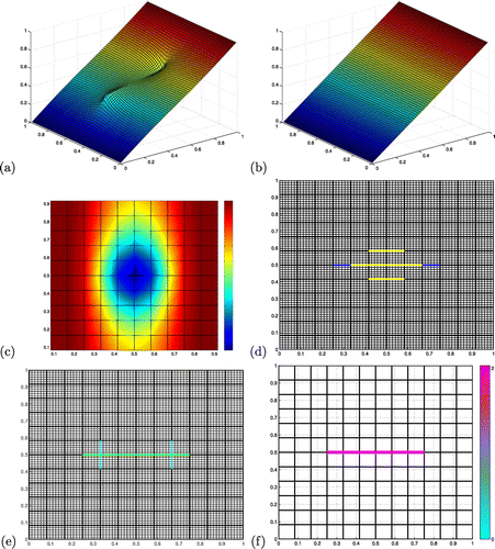
Figure 2. Case of a single fault tangential to the flow. (a) Data pressure, solution of the direct model (36(36) $$\begin{array}{cc}\hfill {\displaystyle \sum _{E\in {\mathcal{E}}_T}{U}_{T,E}}& =f_T,\text{for all}T\in {\mathcal{T}}_h,\hfill \\ \hfill {\displaystyle \frac{\mathit{\kappa }}{2}{U}_{T,E}}& =P_T-P_E,\text{for all}E\notin {\mathcal{F}}_{\mathit{\beta }},T\in {\mathcal{T}}_E,\hfill \\ \hfill {\displaystyle \left(\frac{\mathit{\kappa }}{2}+{\mathit{\beta }}_E\right)U_{T,E}}& =P_T-P_E,\text{for all}E\in {\mathcal{F}}_{\mathit{\beta }},T\in {\mathcal{T}}_E,\hfill \\ \hfill {\displaystyle P_E}& ={\overline{P}}_E,\text{for all}E\in {\mathcal{E}}_h^e,\hfill \\ \hfill {\displaystyle -\sum _{T\in {\mathcal{T}}_E}{U}_{T,E}}& =0,\text{for all}E\notin {\mathcal{F}}_{\mathit{\alpha }},E\in {\mathcal{E}}_h^i,\hfill \\ \hfill {\displaystyle -\sum _{T\in {\mathcal{T}}_E}{U}_{T,E}+{\mathit{\alpha }}_E\sum _{N\in {\mathcal{N}}_E}{V}_{E,N}}& =0,\text{for all}E\in {\mathcal{F}}_{\mathit{\alpha }},\hfill \\ \hfill {\displaystyle \frac{h}{2}{V}_{E,N}}& =P_E-P_N,\text{for all}E\in {\mathcal{F}}_{\mathit{\alpha }},N\in {\mathcal{N}}_E,\hfill \\ \hfill {\displaystyle \sum _{\begin{array}{c}E\in {\mathcal{F}}_{\mathit{\alpha }}\\ E\in {\mathcal{E}}_N\end{array}}{\mathit{\alpha }}_E{V}_{E,N}}& =0,\text{for all}N\in {\mathcal{N}}_{\mathit{\alpha }},\hfill \end{array}$$(36) ) with a fault at $y=0.5$ ($\mathit{\alpha }=2$). (b) Initial pressure, solution of the direct model with no fracture. (c) Distribution of indicators for the long list of elementary candidate faults: the lowest indicator for all six pairs of edges centred in each interior coarse node is represented. (d) In dark blue, the target fault; above in yellow, the selected pairs of edges (three of them are superimposed above the target fault). (e) In light blue, the candidate faults of the short list after aggregation and extension; above in green, the best candidate fault. (f) Best result after minimization for all candidate faults of the short list (the lowest permeabilities are in light blue, and the highest in pink).

6.1. Illustration of the algorithm for the estimation of faults

Let us first consider the simple case of a fault tangential to the flow located in the middle of the domain with $\mathit{\alpha }=2$. The synthetic data are represented in Figure 2(a). The pressure is measured in all elements of the computational mesh (i.e. $N_m=72$). The fracture research mesh corresponds to $N_f=12$, i.e. each coarse edge is made of six fine edges.

The algorithm is initialized with no fracture (${\mathcal{F}}^0=\mathrm{\varnothing }$). The initial direct and adjoint variables $X^0$ and ${\mathrm{\Lambda }}^0$ are computed as solution to (36(36) $$\begin{array}{cc}\hfill {\displaystyle \sum _{E\in {\mathcal{E}}_T}{U}_{T,E}}& =f_T,\text{for all}T\in {\mathcal{T}}_h,\hfill \\ \hfill {\displaystyle \frac{\mathit{\kappa }}{2}{U}_{T,E}}& =P_T-P_E,\text{for all}E\notin {\mathcal{F}}_{\mathit{\beta }},T\in {\mathcal{T}}_E,\hfill \\ \hfill {\displaystyle \left(\frac{\mathit{\kappa }}{2}+{\mathit{\beta }}_E\right)U_{T,E}}& =P_T-P_E,\text{for all}E\in {\mathcal{F}}_{\mathit{\beta }},T\in {\mathcal{T}}_E,\hfill \\ \hfill {\displaystyle P_E}& ={\overline{P}}_E,\text{for all}E\in {\mathcal{E}}_h^e,\hfill \\ \hfill {\displaystyle -\sum _{T\in {\mathcal{T}}_E}{U}_{T,E}}& =0,\text{for all}E\notin {\mathcal{F}}_{\mathit{\alpha }},E\in {\mathcal{E}}_h^i,\hfill \\ \hfill {\displaystyle -\sum _{T\in {\mathcal{T}}_E}{U}_{T,E}+{\mathit{\alpha }}_E\sum _{N\in {\mathcal{N}}_E}{V}_{E,N}}& =0,\text{for all}E\in {\mathcal{F}}_{\mathit{\alpha }},\hfill \\ \hfill {\displaystyle \frac{h}{2}{V}_{E,N}}& =P_E-P_N,\text{for all}E\in {\mathcal{F}}_{\mathit{\alpha }},N\in {\mathcal{N}}_E,\hfill \\ \hfill {\displaystyle \sum _{\begin{array}{c}E\in {\mathcal{F}}_{\mathit{\alpha }}\\ E\in {\mathcal{E}}_N\end{array}}{\mathit{\alpha }}_E{V}_{E,N}}& =0,\text{for all}N\in {\mathcal{N}}_{\mathit{\alpha }},\hfill \end{array}$$(36) ) and (37(37) $$\begin{array}{cc}\hfill {\displaystyle \sum _{E\in {\mathcal{E}}_T}{\mathit{\mu }}_{T,E}}& =P_T-{\overline{P}}_T,\text{for all}T\in {\mathcal{T}}_h,\hfill \\ \hfill {\displaystyle \frac{\mathit{\kappa }}{2}{\mathit{\mu }}_{T,E}}& ={\mathit{\lambda }}_T-{\mathit{\lambda }}_E,\text{for all}E\notin {\mathcal{F}}_{\mathit{\beta }},T\in {\mathcal{T}}_E,\hfill \\ \hfill {\displaystyle \left(\frac{\mathit{\kappa }}{2}+{\mathit{\beta }}_E\right){\mathit{\mu }}_{T,E}}& ={\mathit{\lambda }}_T-{\mathit{\lambda }}_E,\text{for all}E\in {\mathcal{F}}_{\mathit{\beta }},T\in {\mathcal{T}}_E,\hfill \\ \hfill {\displaystyle {\mathit{\lambda }}_E}& =0,\text{for all}E\in {\mathcal{E}}_h^e,\hfill \\ \hfill {\displaystyle -\sum _{T\in {\mathcal{T}}_E}{\mathit{\mu }}_{T,E}}& =0,\text{for all}E\notin {\mathcal{F}}_{\mathit{\alpha }},E\in {\mathcal{E}}_h^i,\hfill \\ \hfill {\displaystyle -\sum _{T\in {\mathcal{T}}_E}{\mathit{\mu }}_{T,E}+{\mathit{\alpha }}_E\sum _{N\in {\mathcal{N}}_E}{\mathit{\nu }}_{E,N}}& =0,\text{for all}E\in {\mathcal{F}}_{\mathit{\alpha }},\hfill \\ \hfill {\displaystyle \frac{h}{2}{\mathit{\nu }}_{E,N}}& ={\mathit{\lambda }}_E-{\mathit{\lambda }}_N,\text{for all}E\in {\mathcal{F}}_{\mathit{\alpha }},E\in {\mathcal{E}}_N,\hfill \\ \hfill {\displaystyle \sum _{\begin{array}{c}E\in {\mathcal{F}}_{\mathit{\alpha }}\\ E\in {\mathcal{E}}_N\end{array}}{\mathit{\alpha }}_E{\mathit{\nu }}_{E,N}}& =0,\text{for all}N\in {\mathcal{N}}_{\mathit{\alpha }}.\hfill \end{array}$$(37) ) with no fracture. The initial pressure is linear (Figure 2(b)).

The first iteration starts with the computation of the fault indicators through (41(41) $$\begin{array}{c}\hfill \begin{array}{ccc}{\displaystyle P_N=\frac{{\sum }_{\begin{array}{c}E\in \mathrm{\Delta }{\mathcal{F}}_{\mathit{\alpha }}\\ E\in {\mathcal{E}}_N\end{array}}{\overline{\mathit{\alpha }}}_E{P}_E}{{\sum }_{\begin{array}{c}E\in \mathrm{\Delta }{\mathcal{F}}_{\mathit{\alpha }}\\ E\in {\mathcal{E}}_N\end{array}}{\overline{\mathit{\alpha }}}_E},}\hfill & {\displaystyle {\mathit{\lambda }}_N=\frac{{\sum }_{\begin{array}{c}E\in \mathrm{\Delta }{\mathcal{F}}_{\mathit{\alpha }}\\ E\in {\mathcal{E}}_N\end{array}}{\overline{\mathit{\alpha }}}_E{\mathit{\lambda }}_E}{{\sum }_{\begin{array}{c}E\in \mathrm{\Delta }{\mathcal{F}}_{\mathit{\alpha }}\\ E\in {\mathcal{E}}_N\end{array}}{\overline{\mathit{\alpha }}}_E},}\hfill & \text{for all}N\in \mathrm{\Delta }{\mathcal{N}}_{\mathit{\alpha }},\hfill \\ {\displaystyle \frac{h}{2}{V}_{E,N}=P_E-P_N,}\hfill & {\displaystyle \frac{h}{2}{\mathit{\nu }}_{E,N}={\mathit{\lambda }}_E-{\mathit{\lambda }}_N,}\hfill & \text{for all}E\in \mathrm{\Delta }{\mathcal{F}}_{\mathit{\alpha }},N\in {\mathcal{N}}_E.\hfill \end{array}\end{array}$$(41) ) and (40(40) $$\begin{array}{c}\hfill {\mathcal{I}}_{\mathit{\alpha }}(\mathrm{\Delta }{\mathcal{F}}_{\mathit{\alpha }})=-\frac{h}{2}\sum _{E\in \mathrm{\Delta }{\mathcal{F}}_{\mathit{\alpha }}}{\overline{\mathit{\alpha }}}_E\sum _{N\in {\mathcal{N}}_E}{V}_{E,N}{\mathit{\nu }}_{E,N},\end{array}$$(40) ) from $X^0$ and ${\mathrm{\Lambda }}^0$ for all elementary candidate faults of the long list made of the 726 pairs of contiguous interior coarse edges of ${\mathcal{T}}_h^c={\mathcal{Q}}^{12,12}$. The cartography of these indicators (Figure 2(c)) shows a nice blue spot in the middle of the domain, right where the target fault is located (remember that good indicators are large negative numbers). Only five pairs of coarse edges have an indicator lower than ${\mathit{\theta }}_{\mathrm{elem}}{\mathcal{I}}_{\mathit{\alpha }}^{\star ,\mathrm{elem}}$; they are parallel and close to the target fault (Figure 2(d)).

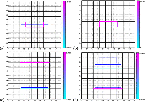
The aggregation stage collapses the three pairs of edges superimposed with the target fault, reducing the number of candidate faults down to three (Figure 2(d)). There is a significant improvement of the indicator as ${\mathcal{I}}_{\mathit{\alpha }}^{\star ,\mathrm{aggr}}\simeq 1.8{\mathcal{I}}_{\mathit{\alpha }}^{\star ,\mathrm{elem}}$.

The extension stage adds one coarse edge at zero, one or two of the endpoints of the aggregated pairs of edges. This multiplies the number of candidate faults by 16 (6 ways to add one edge, 9 ways to add two edges, plus the initial one). The best indicator increases again, by 14%; it corresponds to the target fault (in green in Figure 2(e)). The short list of candidate faults is made of the 7 extended aggregated pairs having an indicator lower than ${\mathit{\theta }}_{\mathrm{ext}}{\mathcal{I}}_{\mathit{\alpha }}^{\star ,\mathrm{ext}}$ (in light blue in Figure 2(e)).

After the minimization of the objective function with respect to the fault parameter (remember that ${\mathit{\epsilon }}_{\mathit{\alpha }}=\mathit{\alpha }$) for all 7 candidate faults of the short list, the best data misfit is divided by a huge factor of ${10}^{16}$ from its initial value. This corresponds to the candidate fault with the best indicator, which happens to be the target fault. And at the minimum, the target value $\mathit{\alpha }=2$ is recovered (Figure 2(f)). The algorithm stops on the convergence criterion.

Figure 3. Case of two faults tangential to the flow. (a) Data pressure, solution of the direct model (36(36) $$\begin{array}{cc}\hfill {\displaystyle \sum _{E\in {\mathcal{E}}_T}{U}_{T,E}}& =f_T,\text{for all}T\in {\mathcal{T}}_h,\hfill \\ \hfill {\displaystyle \frac{\mathit{\kappa }}{2}{U}_{T,E}}& =P_T-P_E,\text{for all}E\notin {\mathcal{F}}_{\mathit{\beta }},T\in {\mathcal{T}}_E,\hfill \\ \hfill {\displaystyle \left(\frac{\mathit{\kappa }}{2}+{\mathit{\beta }}_E\right)U_{T,E}}& =P_T-P_E,\text{for all}E\in {\mathcal{F}}_{\mathit{\beta }},T\in {\mathcal{T}}_E,\hfill \\ \hfill {\displaystyle P_E}& ={\overline{P}}_E,\text{for all}E\in {\mathcal{E}}_h^e,\hfill \\ \hfill {\displaystyle -\sum _{T\in {\mathcal{T}}_E}{U}_{T,E}}& =0,\text{for all}E\notin {\mathcal{F}}_{\mathit{\alpha }},E\in {\mathcal{E}}_h^i,\hfill \\ \hfill {\displaystyle -\sum _{T\in {\mathcal{T}}_E}{U}_{T,E}+{\mathit{\alpha }}_E\sum _{N\in {\mathcal{N}}_E}{V}_{E,N}}& =0,\text{for all}E\in {\mathcal{F}}_{\mathit{\alpha }},\hfill \\ \hfill {\displaystyle \frac{h}{2}{V}_{E,N}}& =P_E-P_N,\text{for all}E\in {\mathcal{F}}_{\mathit{\alpha }},N\in {\mathcal{N}}_E,\hfill \\ \hfill {\displaystyle \sum _{\begin{array}{c}E\in {\mathcal{F}}_{\mathit{\alpha }}\\ E\in {\mathcal{E}}_N\end{array}}{\mathit{\alpha }}_E{V}_{E,N}}& =0,\text{for all}N\in {\mathcal{N}}_{\mathit{\alpha }},\hfill \end{array}$$(36) ) with two faults at $y=0.25$ ($\mathit{\alpha }=2$) and $y=0.75$ ($\mathit{\alpha }=20$). (b) Distribution of indicators for the long list of elementary candidate faults at the first iteration (see Figure 2(c)). (c) Best result after minimization at the first iteration for all candidate faults of the short list. (d) Pressure, solution of the direct model with the estimated fault of (c). (e) Distribution of indicators for the long list of elementary candidate faults at the second iteration. (f) Best result after minimization at the second iteration for all candidate faults of the short list.

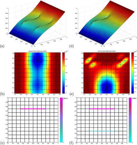
The picture is even more interesting with two faults. Let us now consider the case of two faults tangential to the flow centred at one quarter and at three quarters of the domain with $\mathit{\alpha }=2$ (bottom) and 20 (top). The synthetic data are represented in Figure 3(a). The measurement and fracture meshes remain unchanged ($N_m=72$ and $N_f=12$).

At the first iteration, the cartography of indicators for all elementary candidate faults of the long list shows in Figure 3(b) two blue spots of highly negative values centred at the correct location of the target faults. Moreover, the best indicators are located around the upper fault having the highest permeability (in dark blue). As in the case of a single fault, the aggregation and extension stages multiply the best indicator by a factor of 2, and the best indicator corresponds to the most permeable target fault (the upper one). Again, the best minimizer among the 9 candidate faults of the short list corresponds to the best indicator (the upper target fault). The optimization step decreases the objective function by a factor of 3 only, and at the minimum, a highly overestimated value of about 3300 is recovered for $\mathit{\alpha }$ (Figure 3(c)). Yet, the pressure of Figure 3(d) recovers the main perturbation due to the upper target fault (compare with Figure 3(a)). As the stopping criteria are not satisfied, another iteration is performed.

At the second iteration, the cartography of indicators presents now in Figure 3(e) a strong dark blue spot located at the centre of the least permeable target fault. Clearly, there is nothing left to do around the upper target fault (the area is mostly dark red). The indicators are smaller in magnitude than in the first iteration by a factor of about one third. The optimization step exhibits the best candidate fault of the short list (among 10 of them) as the best minimizer. Again, this best minimizer is exactly the missing lower target fault, the data misfit is divided by a huge factor of $2{10}^{13}$ from its initial value, and the target values $\mathit{\alpha }=20$ and $\mathit{\alpha }=2$ are perfectly recovered (Figure 3(f)). The algorithm stops again on the convergence criterion.

6.2. Beyond the inverse crime

We investigate now less favourable situations with less measurements, and where the synthetic data are no longer in the range of the model used for inversion. The comprehensive campaign of numerical tests is detailed in [34].

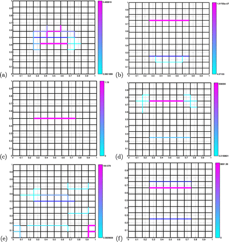
Figure 4. Estimation of faults with less measurement data. The inverted faults are represented with colours ranging from light blue (low permeabilities) to pink (high permeabilities). The target fault is represented in dark blue. (a) Single target fault, no noise, $N_m=6$. (b) Two target faults, no noise, $N_m=8$. (c) Single target fault, 4% noise, $N_m=8$. (d) Two target faults, 4% noise, $N_m=12$. (e) Single target fault, 6% noise, $N_m=8$. (f) Two target faults, 2% noise, $N_m=8$.

Influence of decimation of measurements. When the measurement mesh ${\mathcal{T}}_h^m={\mathcal{Q}}^{N_m,N_m}$ is reduced from $N_m=72$ down to $N_m=8$, numerical tests shown in [34] indicate that the algorithm still provides the target fault as the best candidate fault, and the minimization step still yields the target value of $\mathit{\alpha }$. Moreover, this remains true for target values of $\mathit{\alpha }$ ranging from 0.2 up to 200. For values above 200, the direct model outputs almost the same pressure field: the cost function becomes insensitive to the fault parameter $\mathit{\alpha }$. It is the same for the case of two target faults: down to $N_m=12$, the algorithm still provides the most permeable target fault as the best candidate fault at the first iteration, the least permeable target fault at the second iteration, and then, the minimization step yields the target values of $\mathit{\alpha }$ for both faults.

Problems appear when the distribution of measurement points becomes too loose. At best, the target faults are still located quite accurately, but the minimization step is unable to recover the target values of $\mathit{\alpha }$, and the results may be misevaluated by several orders of magnitude as in the case of two target faults with $N_m=8$ (Figure 4(b)). Or the situation may degenerate progressively: the recovered locations become quite diffuse, but the effective permeabilities can still be quite accurate, as in the case of a single target fault with $N_m=6$ (Figure 4(a)).

Influence of random noise. When adding white Gaussian noise up to a relative noise level of 6% (the perturbation due to the presence of the fault becomes hardly visible by the eye), the algorithm still exhibits the target fault as the best candidate fault, and the minimization step recovers a value of $\mathit{\alpha }=2.01$, almost identical to the target value $\mathit{\alpha }=2$, see [34]. When also decimating the measurements down to $N_m=8$, the algorithm still recovers the target fault as the best candidate fault up to a relative noise level of 4%, and the minimization step yields promising values of 1.5 (with 2% noise) and 1.2 (with 4% noise) for the fault parameter $\mathit{\alpha }$ (Figure 4(c)). The algorithm is not as successful with 6% noise and $N_m=8$: a reasonable estimated fault in the middle (in medium blue) is polluted by a very strong fault in the lower right corner of the domain (Figure 4(e)).

When considering the case of two faults, the conditions are still favourable up to a noise level of 4%: the location of the most permeable fault is recovered at the first iteration and that of the other at the second iteration. Moreover, the minimization step recovers the value $\mathit{\alpha }=17$ for the upper fault and $\mathit{\alpha }=1.99$ for the lower fault, which is still close to the target values 20 and 2. When also decimating the measurements down to $N_m=12$, the algorithm still recovers correctly the least permeable (lower) fault with an excellent inverted value of $\mathit{\alpha }=1.98$, but the most permeable (upper) fault is highly overestimated (values over half a million, Figure 4(d)) and with 4% noise, the location of this fault exhibits artifacts associated with negligible permeabilities under 0.1. For $N_m=8$, only the strongest (upper) fault is estimated with 2% noise, it is located one cell under the target location and the permeability is highly overvalued to about 8700 (Figure 4(f)).

Figure 5. Estimation of faults with coherent noise: the target faults (dark blue) are not carried by the fracture research mesh ($N_f=9$). The inverted faults are represented with colours ranging from light blue (low permeabilities) to pink (high permeabilities). (a) Single target fault, $N_m=72$. (b) Single target fault, $N_m=8$ (c) Two target faults, $N_m=72$. (d) Two target faults, $N_m=8$.

Influence of coherent noise. Finally, we investigate the much more difficult situation where the synthetic pressure data do not belong to the range of the direct model used for inversion, i.e. the global minimum of the objective function is not 0. Of course, we can no longer expect to perfectly retrieve the location and permeability of the target faults, but at least we can hope to recover groups of faults with similar hydrogeological signatures; in fact, values of $\mathit{\alpha }$ are adding up for nearby parallel faults tangential to the flow.

We consider $N_f=9$, hence the target faults located in the middle, or at one quarter and three quarters of the domain, are no longer carried by the fracture research mesh anymore. We also decimate the pressure data from $N_m=72$ down to $N_m=8$. The estimated locations of the faults contain most of the coarse edges of the fracture research mesh that are closest to the target faults. Moreover, with the single target fault, the recovered effective permeabilities range from 1.8 to 3.4, for a target value of 2 (Figure 5(a) and 5(b)). And with the two target faults, the recovered effective permeabilities are higher for the upper fault than for the lower, but they are underestimated up to an order of magnitude (Figures 5(c) and 5(d)): from 1.6 to 2.5 for the most permeable fault (the target value is 20), and from 1.0 to 1.6 for the least one (the target value is 2).

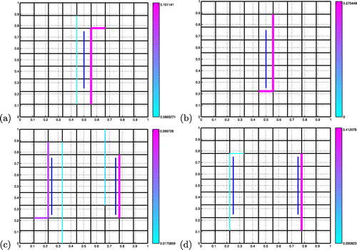
Figure 6. Cases of a single barrier (a)–(c), and of two barriers (d)–(g), normal to the flow. (a) Data pressure, solution of the direct model (36(36) $$\begin{array}{cc}\hfill {\displaystyle \sum _{E\in {\mathcal{E}}_T}{U}_{T,E}}& =f_T,\text{for all}T\in {\mathcal{T}}_h,\hfill \\ \hfill {\displaystyle \frac{\mathit{\kappa }}{2}{U}_{T,E}}& =P_T-P_E,\text{for all}E\notin {\mathcal{F}}_{\mathit{\beta }},T\in {\mathcal{T}}_E,\hfill \\ \hfill {\displaystyle \left(\frac{\mathit{\kappa }}{2}+{\mathit{\beta }}_E\right)U_{T,E}}& =P_T-P_E,\text{for all}E\in {\mathcal{F}}_{\mathit{\beta }},T\in {\mathcal{T}}_E,\hfill \\ \hfill {\displaystyle P_E}& ={\overline{P}}_E,\text{for all}E\in {\mathcal{E}}_h^e,\hfill \\ \hfill {\displaystyle -\sum _{T\in {\mathcal{T}}_E}{U}_{T,E}}& =0,\text{for all}E\notin {\mathcal{F}}_{\mathit{\alpha }},E\in {\mathcal{E}}_h^i,\hfill \\ \hfill {\displaystyle -\sum _{T\in {\mathcal{T}}_E}{U}_{T,E}+{\mathit{\alpha }}_E\sum _{N\in {\mathcal{N}}_E}{V}_{E,N}}& =0,\text{for all}E\in {\mathcal{F}}_{\mathit{\alpha }},\hfill \\ \hfill {\displaystyle \frac{h}{2}{V}_{E,N}}& =P_E-P_N,\text{for all}E\in {\mathcal{F}}_{\mathit{\alpha }},N\in {\mathcal{N}}_E,\hfill \\ \hfill {\displaystyle \sum _{\begin{array}{c}E\in {\mathcal{F}}_{\mathit{\alpha }}\\ E\in {\mathcal{E}}_N\end{array}}{\mathit{\alpha }}_E{V}_{E,N}}& =0,\text{for all}N\in {\mathcal{N}}_{\mathit{\alpha }},\hfill \end{array}$$(36) ) with a barrier at $x=0.5$ ($\mathit{\beta }=2$). (b) Distribution of indicators for the long list of elementary candidate barriers (see Figure 2(c)). (c) Best result after minimization for all candidate barriers of the short list. (d) Data pressure, solution of the direct model (36(36) $$\begin{array}{cc}\hfill {\displaystyle \sum _{E\in {\mathcal{E}}_T}{U}_{T,E}}& =f_T,\text{for all}T\in {\mathcal{T}}_h,\hfill \\ \hfill {\displaystyle \frac{\mathit{\kappa }}{2}{U}_{T,E}}& =P_T-P_E,\text{for all}E\notin {\mathcal{F}}_{\mathit{\beta }},T\in {\mathcal{T}}_E,\hfill \\ \hfill {\displaystyle \left(\frac{\mathit{\kappa }}{2}+{\mathit{\beta }}_E\right)U_{T,E}}& =P_T-P_E,\text{for all}E\in {\mathcal{F}}_{\mathit{\beta }},T\in {\mathcal{T}}_E,\hfill \\ \hfill {\displaystyle P_E}& ={\overline{P}}_E,\text{for all}E\in {\mathcal{E}}_h^e,\hfill \\ \hfill {\displaystyle -\sum _{T\in {\mathcal{T}}_E}{U}_{T,E}}& =0,\text{for all}E\notin {\mathcal{F}}_{\mathit{\alpha }},E\in {\mathcal{E}}_h^i,\hfill \\ \hfill {\displaystyle -\sum _{T\in {\mathcal{T}}_E}{U}_{T,E}+{\mathit{\alpha }}_E\sum _{N\in {\mathcal{N}}_E}{V}_{E,N}}& =0,\text{for all}E\in {\mathcal{F}}_{\mathit{\alpha }},\hfill \\ \hfill {\displaystyle \frac{h}{2}{V}_{E,N}}& =P_E-P_N,\text{for all}E\in {\mathcal{F}}_{\mathit{\alpha }},N\in {\mathcal{N}}_E,\hfill \\ \hfill {\displaystyle \sum _{\begin{array}{c}E\in {\mathcal{F}}_{\mathit{\alpha }}\\ E\in {\mathcal{E}}_N\end{array}}{\mathit{\alpha }}_E{V}_{E,N}}& =0,\text{for all}N\in {\mathcal{N}}_{\mathit{\alpha }},\hfill \end{array}$$(36) ) with two barriers at $x=0.25$ ($\mathit{\beta }=2$) and $x=0.75$ ($\mathit{\beta }=20$). (e) Distribution of indicators at the first iteration. (f) Distribution of indicators at the second iteration. (g) Best result after minimization for all candidate barriers of the short list.

6.3. Estimation of barriers

The case of barriers is quite similar. We present in Figure 6 some tests for one or two barriers normal to the flow. The barrier indicators for the long list of elementary candidate barriers are even more precise: the target barriers are almost already drawn at the beginning of the first iteration of the algorithm in the cartographies of indicators in Figure 6(b) and 6(e). Indeed, the location of the most resistive target barrier is associated with the strongest indicator, and the optimization step picks it up for it produces a perfect fit to the data (Figure 6(c) and 6(g)). Nevertheless, in the case of two barriers, during the extension stage of the second iteration, the location of the weakest target barrier is not associated with the strongest indicator, and it is not even picked up by the optimization step. Consequently, although the best location for the second barrier contains all edges of the least resistive target barrier, the optimization results are not perfect. The recovered values for the resistivity are $\mathit{\beta }=82$ and $\mathit{\beta }=0.41$, instead of the target values 20 and 2; they are quite far, but the hierarchy is correct.

Figure 7. Estimation of barriers with coherent noise: the target barriers (dark blue) are not carried by the fracture research mesh ($N_f=9$). The inverted barriers are represented with colours ranging from light blue (low resistivities) to pink (high resistivities). (a) Single target barrier, $N_m=72$. (b) Single target barrier, $N_m=8$. (c) Two target barriers, $N_m=72$. (d) Two target barriers, $N_m=8$.

When using a fracture research mesh that no longer carries the target barriers ($N_f=9$), the inversion results are still quite reasonable, see Figure 7. We also decimate the pressure data measures from $N_m=72$ down to $N_m=8$. The estimated locations of the barriers contain most of the coarse edges of the fracture research mesh that are closest to the target barriers. After minimization, the recovered effective resistivities (values of $\mathit{\beta }$ are also adding up for nearby parallel barriers normal to the flow) are underestimated by one or two orders of magnitude, but the hierarchy is still preserved.

6.4. Discussion

The first lesson learned from the numerical experiments is that, as hoped, the inversion algorithm presented in Section 5 performs accurately in favourable situations. Indeed, exact fit to synthetic data that are in the range of the inversion model can be reached in a wide variety of situations: for one or two faults tangential to the flow, for a barrier normal to the flow, for a wide range of target parameter values (up to four orders of magnitude), and when loosening the number of distributed measurements (up to a factor of about 80).

Much more interesting is the stability property shown by the algorithm. The recovered fractures remain perfectly located, or at least superimposed with the target location, when adding random noise up to a level of 6% for faults, and of 8% for barriers, see [34]. And this remains true when loosening the number of measurements by a factor of about 80 for up to 4% noise (for faults) and up to 5% noise for barriers. Moreover, when the situation deteriorates a bit more, for instance when the measurement mesh becomes just too loose, when the noise level becomes just too high, or when the target fractures no longer belong to the fracture research mesh, then the location of recovered fractures remains within a distance of no more than a coarse cell from the target location. Furthermore, even when fractures are estimated by several smaller fractures of close location, the value of the recovered effective parameter is of the same order than the target value for single fractures, and the hierarchy in values is kept in the case of two target fractures.

However, the heuristic strategy detailed in Section 5.6 was designed for the case of fault detection, and it may be suboptimal for the estimation of barriers. Indeed, even in the most advantageous case of the inverse crime with full measurements, the indicator step of the algorithm is unable to nominate the target location of the least resistive barrier in the case of two target barriers normal to the flow.

Finally, the amount of measurements necessary to accurately recover the location of fractures may seem prohibitive (64 in our tests). This indicates that one needs a fine enough distribution of measurement to hope solving this difficult inverse problem. Some further experiments could deal with a study of the influence of the location of measurements: a priori information may help driving the measurements in the vicinity of the target fracture in order to reduce their number.

7. Conclusion

The estimation of fractures in porous media from pressure and/or flow data is known to be an ill-posed inverse problem. We propose a new approach for the recovering of both location and hydrogeological properties of a small number of large fractures. The method does not need any remeshing, nor shape derivation.

We have chosen a numerical flow model that treats fractures as interfaces interacting with the surrounding porous matrix, and we have derived a forward model for the simulation of both faults and barriers with vanishing intensities, provided they are located on edges of the simulation mesh. Then, the approach is based on the minimization of an error function that measures the distance between data and simulated measurements.

We have defined specific fracture indicators, whose sign and modulus give the effect on the data misfit of opening any candidate fault or barrier. These indicators give only first-order information, but are computationally inexpensive.

Overparameterization is avoided by restricting the search for fractures to edges of a coarser mesh than the computational grid, and by introducing fractures one at a time. When the data misfit is too high, a short list of new candidate fracture locations is built from a large number of elementary fracture locations that span the entire domain of interest, with the assistance of fracture indicators. The actual enhancement brought by each candidate is computed by optimization, and the best performing fracture is retained.

Numerical tests have been performed on synthetic data corresponding to simple typical situations. They demonstrate the ability of the proposed algorithm to automatically retrieve one or two faults parallel to the flow, or one or two barriers perpendicular to the flow. The algorithm is shown to be fairly stable when noise is added to the data, and when the fracture to be detected is not located on the fracture search mesh.

Notes

No potential conflict of interest was reported by the authors.

References

- Dietrich P, Helmig R, Sauter M, et al. Flow and transport in fractured porous media. Berlin: Springer; 2005.
- Adler PM, Thovert JF, Mourzenko VV. Fractured porous media. Oxford: Oxford University Press; 2013.
- Le Goc R, de Dreuzy JR, Davy P. Statistical characteristics of flow as indicators of channeling in heterogeneous porous and fractured media. Adv Water Res. 2010;33(3):257–269. Available from: http://www.sciencedirect.com/science/article/pii/S0309170809001936.
- Barenblatt GI, Aheltov IP, Kochina IN. Basic concepts in the theory of seepage of homogeneous liquids in fissured rocks. J Appl Math Mech. 1960;24:1286–1303.
- Warren JE, Root PJ. The behavior of naturally fractured reservoirs. Soc Pet Eng J. 1963;245–255.
- Biondi BL. 3D seismic imaging, Investigations in geophysics. Vol. 14. Tulsa (OK): Society of exploration geophysicists; 2006.
- Bimpas M, Anditis A, Uzunoglu N. Integrated high resolution imaging radar and decision support system for the rehabilitation of water pipelines. London: IWA publishing; 2010.
- Baca RG, Arnett RC, Langford DW. Modelling fluid flow in fracture-porous rock masses by finite-element techniques. Int J Num Methods Fluids. 1984;4:337–348.
- Karimi-Fard M, Firoozabadi A. Numerical simulation of water injection in fractured media using the discrete-fracture model and the galerkin method. SPE REE. 2003;117–126.
- Karimi-Fard M, Durlofsky LJ, Aziz K. An efficient discrete fracture model applicable for general purpose reservoir simulators. SPE J. 2004;227–236.
- Reichenberger V, Jakobs H, Bastian P, Helmig R. A mixed-dimensional finite volume method for multiphase flow in fractured porous media. Adv Water Res. 2006;29(7):1020–1036.
- Kim Deo. Finite element discrete-fracture model for multiphase flow in porous media. AIChE J. 2006;463(6):1120–1130.
- Hoteit H, Firoozabadi A. An efficient numerical model for incompressible twophase flow in fractured media. Adv Water Res. 2008;31:891–905.
- Martin V, Jaffré J, Roberts JE. Modeling fractures and barriers as interfaces for flow in porous media. SIAM J Sci Comput. 2005;26(5):1667–1691.
- Angot P, Boyer F, Hubert F. Asymptotic and numerical modelling of flows in fractured porous media. M2AN. 2009;43(2):239–275.
- Lesinigo M, D’Angelo C, Quarteroni A. A multiscale darcy-brinkman model for fluid flow in fractured porous media. Num Math. 2011;117(4):717–752.
- D’Angelo C, Scotti A. A mixed finite element method for Darcy flow in fractured porous media with non-matching grids. M2AN Math Model Numer Anal. 2011;46(2):465–489.
- Frih N, Martin V, Roberts JE, et al. Modeling fractures as interfaces with non-matching grids. Computational Geosciences. 2012;16:1043–1060. DOI:10.1007/s10596-012-9302-6.
- Tunc X, Faille I, Gallouët T, et al. A model for conductive faults with non-matching grids. Computational Geosciences. 2012;16(2):277–296. DOI:10.1007/s10596-011-9267-x.
- Knabner P, Roberts JE. Mathematical analysis of a discrete fracture model coupling darcy flow in the matrix with darcy-forchheimer flow in the fracture. ESAIM M2AN. 2014;48:1451–1472.
- Brenner K, Groza M, Guichard C, et al. Gradient discretization of hybrid dimensional Darcy flows in fractured porous media. In: Fuhrmann J, Ohlberger M, Rohde C, editors. Finite volumes for complex applications VII Elliptic parabolic and hyperbolic problems. Springer Proceedings in Mathematics & Statistics. Vol. 78. Cham: Springer; 2014. p. 527–535. DOI:10.1007/978-3-319-05591-6\_52.
- Brenner K, Groza M, Guichard C, et al. Vertex approximate gradient scheme for hybrid dimensional two-phase Darcy flows in fractured porous media. ESAIM Math Model Numer Anal. 2015;49(2):303–330. DOI:10.1051/m2an/2014034.
- Alboin C, Jaffré J, Roberts JE, et al. Domain decomposition for flow in porous fractured media. In: Lai CH, Bjorstad PE, Cross M, et al, editors. Domain decomposition methods in sciences and engineering. Bergen: Domain Decomposition Press; 1999. p. 365–373.
- Jaffré J, Martin V, Roberts JE. Generalized cell-centered finite volume methods for flow in porous media with faults. In: Herbin R, Kr{\"o}ner D, editors. Finite volumes for complex applications, III. Paris: Hermes Science Publication; 2002. p. 367–364.
- Faille I, Flauraud E, Nataf F, et al. A new fault model in geological basin modelling, application to finite volume scheme and domain decomposition methods. In: Herbin R, Kroner D, editors. Finite volumes for complex applications III. Paris: Hermés Penton Sci; 2002. p. 543–550.
- Tunc X, Faille I, Gallouët T, et al. A model for conductive faults with non-matching grids. Comput Geosci. 2011;16(2):277–296. DOI:10.1007/s10596-011-9267-x.
- Moreles F, Showalter RE. The narrow fracture approximation by channeled flow. JMAA. 2010;365(1):320–331.
- Frih N, Roberts JE, Saâda A. Modeling fractures as interfaces: a model for Forchheimer fractures. Comput Geosci. 2008;12:91–104.
- Engl HW, Hanke M, Neubauer A. Regularization of inverse problems. Mathematics and its applications. Vol. 375. Dordrecht: Kluwer Academic; 1996. DOI:10.1007/978-94-009-1740-8
- Chavent G. Nonlinear least squares for inverse problems. Scientific computation. New York (NY): Springer; 2009; theoretical foundations and step-by-step guide for applications.
- Ameur H, Chavent G, Jaffré J. Refinement and coarsening indicators for adaptive parametrization: application to the estimation of hydraulic transmissivities. Inverse Prob. 2002;18(3):775–794. DOI:10.1088/0266-5611/18/3/317.
- Ameur H, Clément F, Weis P, et al. The multidimensional refinement indicators algorithm for optimal parameterization. J Inverse Ill-Posed Prob. 2008;16(2):107–126. DOI:10.1515/JIIP.2008.008.
- Ameur H, Chavent G, Clément F, et al. Image segmentation with multidimensional refinement indicators. Inverse Prob Sci Eng. 2011;19(5):577–597; special Issue: Proceedings of the 5th International Conference on Inverse Problems: Modeling and Simulation; 2010 May 24--29; Antalya, Turkey. Available from: http://dx.doi.org/10.1080/17415977.2011.579609.
- Cheikh F. Identification des fractures dans un milieu poreux [dissertation]. ENIT Tunis (Tunisia), U. Paris 6 (France); Forthcoming. French.
- Chavent G, Roberts JE. A unified physical presentation of mixed, mixed-hybrid finite elements and standard finite difference approximations for the determination of velocities in aterflow problems. Adv Water Res. 1991;14(6):329–348.