
 ?Mathematical formulae have been encoded as MathML and are displayed in this HTML version using MathJax in order to improve their display. Uncheck the box to turn MathJax off. This feature requires Javascript. Click on a formula to zoom.
Abstract
We present a model for the dynamics of phytoplankton aggregates and their interaction with the environment in a well-mixed reactor or surface layer of a water column. The biophysical problem yields a nonlinear partial differential equation coupled with a general system of ordinary differential equations. We first develop a finite difference scheme for approximating the solution of this model. Then convergence results are established for the finite difference method and existence-uniqueness of solutions are obtained. A least-squares parameter estimation method is presented to illustrate the performance of the model against a real dataset, and to highlight the effects of aggregate growth on algal bloom dynamics and nutrient consumption rates. The model is well-suited to complement microcosm studies and can accommodate the effects of a wide range of environmental conditions.
1. Introduction
Ample research has been undertaken to understand the role of phytoplankton in a variety of applied settings [Citation1–Citation8]. Phytoplankton represent an important layer in the aquatic food web of marine and freshwater ecosystems throughout the world [Citation9]. Given the vast scope of natural phytoplankton systems (e.g. rivers, reservoirs, and oceans), it is challenging to address what-if type questions in a realistic setting [Citation10,Citation11]. Recent demonstrations show the potential of in situ algal stimulation by nutrient seeding in the open ocean at small scales [Citation12,Citation13]. However, seeding activities are challenged by logistics and other practical concerns associated with bloom stimulation in the natural environment. On the smaller scale of chemical engineering the development of commercially-viable algae-based clean energy alternatives and other green product technologies are also hindered by the difficulty of extrapolating laboratory results to practical scales of production [Citation14–Citation21].
Mathematical models can address some of the challenges associated with phytoplankton population dynamics, since they can include many of the variables which are too complex to investigate in practical settings. Phytoplankton populations can be modeled as a collection of irregularly-shaped particle aggregates bound together by some organic glue. The particles increase in size either by biological cell division or the physical process of coagulation when they encounter other suspended particles. Since phytoplankton growth depends on photosynthesis, cell death may occur at the core of large aggregates while cell division may persist on active portions of the particle surface. So, in general, only a portion of the aggregate experiences growth and uptake of nutrients from the water column and this phenomenon is challenging to model accurately.
Past work for the development of size-structured phytoplankton aggregation models and/or their numerical approximations includes [Citation22–Citation29]. Researchers have focused on establishing existence-uniqueness of solutions to the classical coagulation-fragmentation problem and an investigation of their long-term behavior [Citation30–Citation33]. Understanding what controls the distribution of phytoplankton and nutrient dyamics is a major challenge facing contemporary biological oceanographers, and such investigations could benefit from models capable of accomodating a wide variety of factors [Citation34–Citation37]. Previous studies have implemented the size-structured approach to model the behavior of flocculating bacterial and microbial aggregates in suspension systems [Citation38–Citation40]. However, to the best of our knowledge no size-structured model exists which includes a general array of environmental variables and numerically investigates the sensitivity of algal bloom formation and nutrient depletion in response to the interaction of coagulation, aggregate growth, and reproduction rates in a physically realistic context.
Our aim is to introduce a structured population model for phytoplankton which includes a general vector of environmental variables, growth of particle aggregates, reproduction, and coagulation in which the model parameters depend on the generalized environment. In addition to presenting the model, the objectives of this paper are (1) to present a first-order finite difference numerical approximation and to develop new innovative techniques to treat the nonlinearity associated with the coagulation term and to establish the necessary estimates for convergence of the first-order finite difference scheme, (2) to establish existence and uniqueness of the solution to the model, (3) to accurately model growth within aggregates and (4) to study the sensitivity of the model to its parameters and to utilize a least-squares approach to fit the model to a tank experiment data set.
This paper is organized as follows: in Section 2 we introduce the general nonlinear model and in Section 3 we introduce the notation and assumptions used in the forthcoming analysis. In Section 4 we setup a finite difference approximation and establish a series of technical lemmas using standard compactness arguments for scalar conservation laws in the spirit of [Citation41] (Chapter 16) to show that the finite difference scheme converges to a weak bounded variation (BV) solution to the model. In Section 5 we show that the scheme converges to the unique BV solution. In Section 6 we develop sub-models for the vital rates and in Section 7 we setup a least-squares problem to compare the model to a dataset. This least-squares problem involves finding optimal parameter values for aggregate growth, and the fraction of live vs. dead material. In Section 8 we provide some concluding remarks. The details of the technical proofs are provided in the Appendix 1.
2. The model
Consider the well-mixed surface layer of a geographic parcel of water (commonly referred to as the water column in environmental engineering) and a population ofphytoplankton particles having number density per unit size u. The following model describes the size-structured dynamics of the system(2.1)
(2.1)
where(2.2)
(2.2)
and(2.3)
(2.3)
The term A(u) is used to model the particle coalescence process [Citation42,Citation43]. The function represents the rate at which particles of size x coagulate with particles of size s to yield particles of size
at a given moment in time t. The parameter g is the size-specific growth rate of a particle aggregate, and R is the individual mortality, or rate of disappearance of aggregates of size x from the surface layer. The function F measures the addition of particles of smallest size from an outside source and
is the individual reproduction rate of newborn cells. The term
is a vector containing the environmental variables (e.g. temperature, water chemistry, grazing, light intensity, nutrients, etc.) all of which interact with each other and the particle population. The components of the vector
are
and the functions
and
are nonlinear environmental source and mortality terms, respectively which also depend on the particle population. The evolution of the environment is governed by an m-dimensional system of nonlinear ordinary differential equations. The variable
represents some weighted average of the population with weight function
. The variables
and
are weighted averages of the population and weight functions, respectively which interact with the environmental variables
. In Section 6 and Table we provide an example featuring specific sub-models, descriptions, and a summary of units for model variables and parameters in the SIGMA tank phytoplankton experiment [Citation23].
The model (Equation2.1(2.1)
(2.1) ) studied in this paper utilizes concepts developed by Smoluchowski to investigate particle dynamics in the presence of coagulation [Citation44]. It is a combination of the continuous version of the coagulation model used to study aggregation in well-mixed particle systems [Citation45] and the classical Sinko-Streifer model of size-structured populations subject to growth, mortality, and reproduction [Citation46]. This combination of factors takes into account the biological and physical variables which determine the fate of an individual phytoplankton aggregate. The model also generalizes the concept of environment by including an arbitrary number of variables (
) which are coupled with the vital rates of the particle population. This yields a quasilinear hyperbolic partial differential equation coupled with a system of nonlinear ordinary differential equations containing nonlocal terms. The terms
and
are nonlocal in the sense that they depend on the entire particle population rather than the (local) population density at a given point. Theoretically, this model belongs to the class of 1-dimensional scalar conservation laws in which the conserved variable is the population density of cell aggregates. It is well known that solutions to the 1-dimensional particle aggregation problem can exhibit gelation (i.e. emergence of a particle having infinite size) in finite time for certain specific forms of the coagulation function. Gelation is not known to occur in real phytoplankton systems and we will establish conditions which guarantee the absence of gel-forming solutions to the model (Equation2.1
(2.1)
(2.1) ). Also, in most applications one should expect that the initial data
will contain gaps and noise (i.e. discontinuities), and these considerations motivate us to pursue weak solutions in the space of functions having bounded total variation, BV.
3. Assumptions and weak solution definition
Let ,
. We denote by
the space of continuous functions on
, by
the space of continuously differentiable functions on
, and by
the space of functions with bounded total variation on
. Recall that a function f over
is said to be locally Lipschitz continuous if for every
there exists a neighborhood U of x such that f restricted to U is Lipschitz continuous. We denote by
the space of locally Lipschitz continuous functions on
and by
the space of Lipschitz continuous functions on
. Throughout the paper we will use the shorthand notation
to represent the Lipschitz constant for a Lipchitz continuous function f. For example,
will denote the Lipschitz constant for the function
and we omit the index
when denoting the maximal Lipschitz constant for a given function over all environmental factors, i.e.
.
Let and
be sufficiently large positive constants. Denote by
the positive cone of
,
and let
,
,
, and
. Throughout the discussion we impose the following conditions on our model parameters in (Equation2.1
(2.1)
(2.1) ), for each
.
| (B1) | The function | ||||
| (B2) |
| ||||
| (B3) |
| ||||
| (B4) |
| ||||
| (B5) | For any sufficiently small | ||||
| (B6) |
| ||||
| (B7) |
| ||||
| (B8) | The nonnegative weight functions | ||||
| (B9) |
| ||||
| (B10) |
| ||||
Definition 3.1:
An -tuple of functions
is called a weak solution to problem (Equation2.1
(2.1)
(2.1) ) if for
,
and the following holds for every test function
for all
:
and
4. Difference approximations
Suppose that the intervals and [0, T] are divided into N and L subintervals respectively. The following notation will be used throughout this section:
, and
denote the spatial and time mesh sizes respectively. The mesh points are given by
, and
. For convenience of notation we apply equal mesh sizes in the x dimension and a uniform time step. The proof of convergence can be established in a similar manner using a more general non-uniform mesh. We denote by
,
,
, and
, the finite difference approximations of
,
,
, and
, respectively. The values of the model parameters evaluated at the mesh points are given below,
defined for all ,
, and
.
We define the and
norms and the TV (total variation) seminorm of the grid functions
and
by
for . We also adopt the following nonstandard first-order finite difference scheme for
:
(4.1)
(4.1)
First observe that the first equation in (Equation4.1(4.1)
(4.1) ) has a unique nonnegative algebraic solution and this result satisfies a biological requirement. This can be seen by multiplying the first row of (Equation4.1
(4.1)
(4.1) ) by
and rewriting equation to obtain
(4.2)
(4.2)
All terms on the right hand side of (Equation4.2(4.2)
(4.2) ) are nonnegative by the nonnegativity assumption (B9) on the initial data
. Furthermore, the solution to (Equation4.2
(4.2)
(4.2) ) is obtained by a left-to-right substitution process. From assumptions (B3), (B4), and (B9), the algebraic solution to the system of ordinary differential equations given by the third equation in (Equation4.1
(4.1)
(4.1) ) is also nonnegative since this equation can be rewritten as
(4.3)
(4.3)
4.1. Estimates for the finite difference approximations
The particle coagulation problem (Equation2.1(2.1)
(2.1) ) presents mathematical difficulties which are not present in the classical nonlinear Sinko-Streifer or McKendrick von-Forester type structured models. In the Sinko-Streifer size-structured model, individuals may advance in size only through the (continuous) process of biological growth. However, in a particle system subject to aggregation, coagulation causes individual particles to spontaneously increase in size via coalescence and this generally requires an unbounded region to ensure that no particles escape the domain. In numerical simulations and the problem considered here, we truncate the problem to a bounded domain
instead of the classical unbounded domain
used to study general particle aggregation problems. Since the coagulation process manufactures particles of increasing size, in order to prevent the unphysical emergence of a particle of infinite size (i.e. super-particle) in the context of phytoplankton aggregation, we require that
if
. The next challenge is to ensure the conservation of particles. In the continuous case, a straightforward calculation establishes the following result,
and hence in the absence of reproduction, mortality, and immigration (i.e. ), the total number of particles in the system satisfies
(4.4)
(4.4)
which is an expression which measures the rate of change of the number of particles in the system. Physically this result states that in the absence of reproduction, the coagulation process reduces the total number of particles over time. This is an important result and the following lemma shows that it also holds in the discrete case as a result of the implicit differencing applied to the quadratic term on the right hand side in the first row of Equation4.1(4.1)
(4.1) . The result is established below.
Lemma 4.1:
Assume that is nonnegative. Then we have the following:
(4.5)
(4.5)
for any .
Proof See Appendix 1.
Next we will establish an estimate on the finite difference scheme. One notable consequence of the
estimate is that it ensures the absence of gelation (e.g. [Citation47]). This is a biologically realisitic requirement for numerical solutions of the phytoplankton problem.
Lemma 4.2:
The scheme is bounded in , i.e. there exists a constant
such that for all
,
Proof See Appendix 1.
Note that from the inequality established in Lemma 4.2 we have,
and similarly . Thus, using (B1)-(B10), we obtain a uniform upper bound on the parameters
over the compact set
. For convenience we denote this bound by
as well. Next we establish an
stability bound on the numerical approximations.
Lemma 4.3:
There exists a constant such that if
satisfies
,
Proof See Appendix 1.
Lemma 4.4:
There exists positive constants and
, independent of
and
, such that
For all
and
For all
For all
For all
Proof See Appendix 1.
Next we establish an important property of the numerical scheme. In particular, we show that the scheme has bounded total variation.
Lemma 4.5:
If satisfies
, there exists a constant
such that
for every .
Proof See Appendix 1.
We now show that our difference approximations and
are
-Lipschitz in t.
Lemma 4.6:
There exists a constant , independent of
and
such that for
,
Proof See Appendix 1.
5. Existence and uniqueness of the weak solution
Following [Citation41] (Chapter 16, p.275–279) we define a family of functions by extending the finite difference approximations
in (Equation4.1
(4.1)
(4.1) ) to piecewise constant functions and a family of functions
by extending the finite difference approximations
in (Equation4.1
(4.1)
(4.1) ) to piecewise linear functions as follows:
(5.1)
(5.1)
Then the set of functions
is (sequentially) compact in the topology of
and the set of functions
is (sequentially) compact in the topology of C([0, T]) and we have the following Theorem.
Theorem 5.1:
For , there exists a subsequence
which converges to a function of bounded total variation
, and a subsequence
which converges to a function
in the sense that for all
and
as .
Proof See Appendix 1.
Theorem 5.2:
The limit functions u and constructed by the finite difference scheme in Theorem () define a weak solution of the model (Equation2.1
(2.1)
(2.1) ) and satisfy
(5.2)
(5.2)
for some constant and each
.
Proof See Appendix 1.
Towards demonstrating that the weak solution is unique, we first establish the following lemma which guarantees the continuous dependence of the solutions and
to the coupled PDE system (Equation2.1
(2.1)
(2.1) ) with respect to the initial conditions
.
Lemma 5.3:
Let ,
,
and
be the solutions of (Equation2.1
(2.1)
(2.1) ) corresponding to the initial conditions
,
,
, and
respectively. Assume that
is chosen so that
. Then there exists a constant
such that
Proof See Appendix 1.
Lemma 5.3 is then applied to prove that the weak solution defined in Theorems () and () is unique. Using techniques similar to those presented in [Citation48], and the results established in Lemma 5.3, we arrive at the following result for some constant ,
(5.3)
(5.3)
Theorem 5.4:
Suppose u, and
,
are two bounded variation weak solutions of (Equation2.1
(2.1)
(2.1) ) corresponding to the initial conditions
,
and
,
respectively. Then there exists a constant
such that
(5.4)
(5.4)
Proof The result follows immediately by applying the Gronwall inequality to Equation (Equation5.3(5.3)
(5.3) ) and letting
.
6. Development of sub-models for the vital rates
In this section we parameterize the model (Equation2.1(2.1)
(2.1) ) to numerically investigate the role of the phytoplankton aggregate growth rate process on algae bloom development and nutrient dynamics. The basis of this biogeochemical application is the 1993 SIGMA reactor experiment [Citation23,Citation49]. The researchers employed a version of the model (Equation2.1
(2.1)
(2.1) ) which was used to investigate the effects of coagulation on the population dynamics of a phytoplankton community (mostly diatoms, i.e. Chaetoceros sp., Thalassiosira sp.) subject to nutrient depletion. The model results matched the observations well, and size-structured model parameters were made available as a result of this experiment. The key parameters under investigation in the SIGMA experiment were the stickiness parameter and the contact efficiency power relationship. An individual based approach using only single cells was used to track nutrient depletion, and nutrient uptake was assumed to be a function of the single cells only. Our goal is to enhance the SIGMA reactor aggregation model [Citation23] to include aggregate growth and reproduction and to demonstrate the effect of including these terms on the coupled particle and nutrient dynamics.
In order to extend the model presented in [Citation23] we assume that cell aggregates in general can be partitioned into living material on the particle surface and non-living material at the core. The analysis of a size-structured model which includes growth and aggregation has been investigated using the finite element method (FEM) (see, [Citation25]). The numerical results established in [Citation25] suggest that growth and aggregation are processes that enhance each other and the inclusion of growth increases the formation of large aggregates compared to models which include aggregation only. The following analysis extends the previous work by investigating the role of multi-celled aggregate growth, coagulation and nutrient availability in a realistic setting. We begin by deriving concrete expressions for the vital rate parameters which are necessary to perform the numerical trials.
Note that in this application, since the reactor system is closed and well-mixed throughout the experiment (i.e. negligible sedimentation effects), and the effects of grazing were negligible. Also,
throughout the simulation since the tank was not artificially seeded with single cells after the beginning of the experiment. We also point out that we understand the slight abuse of notation in this section because some parameters described herein are not as general as those described in (Equation2.1
(2.1)
(2.1) ).
Consider an individual phytoplankton cell aggregate of volume x subject to cell growth, coagulation, and encapsulation. Encapsulation is assumed to occur when cell aggregates become sufficiently large in size to the point where cell division is arrested in portions of the aggregate (Figure ). As indicated in [Citation25], the maximum specific growth rate of single cells based on experimental data is approximately 1.2 per day where the specific growth rate is the ratio of the growth rate to the total size of the aggregate. Encapsulation would then be reflected in specific growth rates smaller than unity based on the assumption that a necrotic portion (i.e. core) of the aggregate does not undergo photosynthesis (e.g. as a result of inadequate light exposure or nutrients). This assumption has been applied to the numerical investigation of aggregating bacterial systems in [Citation39]. The following derivation is in the spirit of the arguments presented in [Citation22,Citation23]. The forthcoming assumptions are made in an effort to develop biologically relevant expressions of the size structured vital rate parameters:
| (N1) | The total volume of a cell aggregate can be partitioned into core volume and active volume, i.e. | ||||
| (N2) | The core volume | ||||
| (N3) | The active volume, | ||||
| (N4) | Nutrient uptake and cell division occurs only in the active portion of the aggregate. The nutrient uptake rate is proportional to the total active biomass in the system. | ||||
| (N5) | The total aggregate growth rate, | ||||
| (N6) | The total aggregate growth rate is the sum of attached growth | ||||
where and the exponent
is a parameter which determines the influence of encapsulation with larger values corresponding to greater resistance to the effects of encapsulation. The parameter
represents the growth rate of the smallest sized aggregate considered in the analysis. The constant
is a parameter which also reflects the effects of encapsulation with larger values corresponding to a greater resistance to the effects of encapsulation. The attached growth rate is defined by
where
. Conversely, the reproduction rate has the following form
where is a reproduction factor.
Nutrient concentration was the only environmental variable considered in the trial and hence in (Equation2.1
(2.1)
(2.1) ). From hereinafter, the symbol
is used to model the average nutrient concentration in the tank at time t. The nutrient reduction rate in the reactor at time t is assumed to be proportional to the active biomass in the following manner,
(6.1)
(6.1)
Here is a nutrient consumption parameter. We then modify (Equation6.1
(6.1)
(6.1) ) by imposing a Monod-type function to model the self-limiting effects of nutrient consumption during bloom formation to obtain
(6.2)
(6.2)
where is the nutrient consumption rate limiter. We also apply a growth rate limiter
to the growth function where
is a small constant which reflects the presence of alternative nutrients once nitrates are depleted (e.g. Figure 5, [Citation49]). Using (Equation6.2
(6.2)
(6.2) ) we are able to simulate the nutrient dynamics coupled with the size-structured phytoplankton dynamics in the reactor. The particle density is modeled using the approach presented in [Citation22] and is coupled with (Equation6.2
(6.2)
(6.2) ) through the nutrient-dependent growth and birth rate functions. The nutrient dependent attached growth rate (Figure ) is given by
(6.3)
(6.3)
and the reproduction term (i.e. left boundary condition) is given by
The coagulation function is based on the formulation given in [Citation23],
Here, is the sticking probability, and
and
are the individual collision rates due to shear and differential settling of particles, respectively as defined below [Citation23,Citation24],
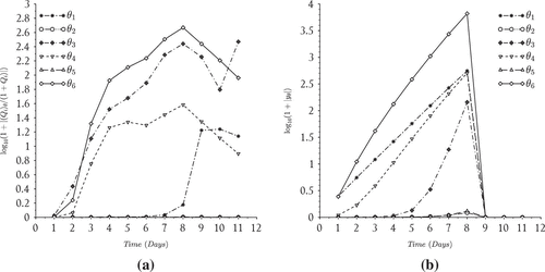
Figure 1. Modeled phytoplankton aggregate growth rates. (a) Particle growth parameters, (b) Particle doubling rates.
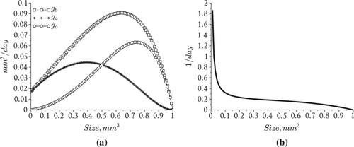
Figure 2. Coagulation rates, .
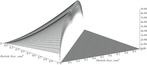
Here, and
denote the contact efficiencies due to shear and differential settling respectively. The parameter
represents the fall velocity of a particle of volume x and
represents the diameter of a particle having volume x. See Figure for a graph of the coagulation rates. The remaining constants and variables used in the model are summarized in Table .
Table 1. Variables and parameter values used in the model.
7. Least-squares method and parameter estimation results
In this section, we apply the vital rates and nutrient consumption formulation outlined in Section 6 to the model (Equation2.1(2.1)
(2.1) ). We then utilize the finite difference scheme (Equation4.1
(4.1)
(4.1) ) to solve a least squares parameter estimation problem that compares the model output to real data. The objective is to obtain a suitable set of parameters from which we can gain insight on the interaction between aggregate growth, coagulation, and nutrient dynamics and evaluate the sensitivity of the model outputs near the optimal parameter values. Given that the model contains many parameters, such an exercise may be useful both in experimental design and also in identifying the most significant factors driving the overall dynamics of the system.
The focus of this section is the study of the following parameter identification problem: given observations and
which correspond to the measured daily average nutrient concentration and total particle number in the size interval
respectively at time
days from the beginning of the simulation, find a parameter
which minimizes the least squares cost functional
defined by
(7.1)
(7.1)
where the subscript denotes the population histogram bin corresponding to the particle size class
. The vector of parameters to be estimated is
, where
and
. The factor
is introduced to balance the objective function since the quantities of the nutrients and phytoplankton have different units and relative magnitudes.
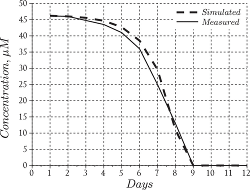
Figure 3. Nutrient model performance.
To compute minimizers for the above inverse problem we first approximate the objective function (Equation7.1(7.1)
(7.1) ) in the following manner:
where the functions and
as defined in (Equation5.1
(5.1)
(5.1) ) are obtained from solving the difference equations (Equation4.1
(4.1)
(4.1) ). For the remainder of this section we will use the notation for simplicity,
For the computations presented below we divide the model domain using uniformly spaced mesh points with
days and
. The computational point spacing along the x-axis was consistent with the numerical trials presented in [Citation23], i.e.
, yielding
and
where
. The size bins were defined as
. The computational time step is selected as follows:
and
simulation steps yielding
and
days respectively.
We point out that the raw experimental data was not directly available. As a result the observed nutrient data was digitized from the figures provided in [Citation23]. Similarly, the observed particle histogram data
was inferred from the figures presented in [Citation29] noting that the non-uniform measurements were converted to a uniform particle size bin in order to compare the measurements with the numerical model results. The initial conditions for both the nutrients and the particle densities were inferred from the digitized experimental data. A series of preliminary numerical trials were performed first to determine the weight factor
. This was done for convenience, but in general the weight parameter
may be estimated from the data directly using the methods discussed in [Citation50]. The least squares minimization problem was then numerically solved using the standard Fortran LMDIF1 minimization package.
The final squared residuals for the nutrients and the phytoplankton population were 36.4 and 22.4, respectively. This shows that our choice of produces residuals which are within the same order of magnitude for both datasets. In Figures and we present the data fits for the nutrients and the phytoplankton aggregates that resulted from solving the above least-squares problem and in Table we present the values of the estimated parameters.
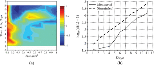
The results suggest that the model performed reasonably well in capturing the overall behavior of the bloom, i.e. formation time for large aggregates (day 6) and order of magnitude for particles in the middle of the size spectrum (Figure ). The nutrient model also performed reasonably well particularly in tracking the disappearance rate and the time at which nitrates fell below detection limits (day 9) inside the tank (Figure ). However, the model overestimated the total particle numbers during the middle of the experiment but converged with the measurements towards the end of the simulation run (Figure ). We also point out that the model tends to overestimate the total particles until day 8 at which time the model begins to underestimate the aggregates uniformly except for particles in the size range smaller than 0.2 . After this time the modeled histogram generally fell short of the measurements over the final days of the simulation. We point out that the total particle numbers converged at the end of the bloom which suggests the results may be improved in the future by including an additional process which has the ability to distribute particles uniformly across the size range. Such a process should theoretically operate throughout the course of the bloom even when growth and reproduction processes are restricted by a lack of nutrients. A more realistic scenario may be that cell aggregates fracture according to a distribution of sizes, particularly in mixed (i.e. turbulent) environments such as those maintained during the SIGMA experiment. Distributed breakage leads to a fragmentation term which should be investigated in future efforts to improve the model predictions.
The calculation of standard errors and sensitivity for the estimated parameters follows the methods outlined in [Citation51]. In particular, to compute the variance in the estimated vector of parameters, , we start by computing the sensitivity matrix given by
where . To compute
and
, (
and
) we used the following approximation
for days from the beginning of the experiment. The increment
was used in the approximation of the sensitivity matrix Z. Additional simulations were taken to investigate the impact of the step size on the sensitivity calculations. The results suggest that reducing
beyond
did not significantly alter the sensitivity metrics. An alternative method for computing derivative approximations which addresses the ‘step size dilemma’ is discussed in [Citation52].
Under the standard assumptions of classical nonlinear regression theory, we know that if the errors satisfy
where
is the difference between the model and the observations at time
, then the least-squares estimate
is expected to be asymptotically normally distributed. In particular, for large samples, we may assume
(7.2)
(7.2)
where is the true vector of parameters and
is the true covariance matrix. Since
and
are not available, we follow a standard statistical practice in which we substitute the computed estimate
for
and approximate the error variance
in (Equation7.2
(7.2)
(7.2) ) using the residuals given by
which are computed using the finite difference approximation as follows:
The covariance matrix is then approximated by
and the standard errors are approximated by taking the diagonal elements of the covariance matrix of the approximations, i.e. for each parameter
respectively. The coefficient of variation (CV) is defined as
, respectively. The CV is also provided in Table for an assessment of the degree of uncertainty in the estimates. The standard errors suggest that the greatest degree of uncertainty was found in the estimate for the encapsulation exponent,
.
Figure 4. Phytoplankton bloom formation: (a) measurements adapted from Figure 2 in [Citation23] and (b) model results.
![Figure 4. Phytoplankton bloom formation: (a) measurements adapted from Figure 2 in [Citation23] and (b) model results.](/cms/asset/14331da1-da7b-4fce-b9d5-fdbffca4dad3/gipe_a_1310856_f0004_oc.gif)
Figure 5. Phytoplankton bloom formation: (a) error levels given by and (b) incremental total particle comparison.
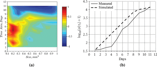
Table 2. Least-squares parameter values and their standard errors.
The sensitivity plots given in Figure suggest that the particle histograms (0.5 size class) were most sensitive to the growth rate of the smallest aggregate
, the sticking probability
, and the aggregate encapsulation factor
respectively. This outcome underscores the importance of the aggregate growth process in modeling phytoplankton bloom and nutrient dynamics in general. The histogram was relatively insensitive to perturbations in the reproduction factor
or the encapsulation exponent
. The nutrient dynamics were sensitive to the aggregate growth parameters as well as the nutrient consumption parameter. The relative sensitivities of the nutrient dynamics with respect to all parameters approached zero after the nutrients fell below detection limits in the tank (day 9). We point out that the sensitivity of the histogram of mid-sized particles with respect to changes in the nutrient consumption rate
increased from virtually zero after nutrients fell below the detection limit. This suggests a possible time delay between the nutrient dynamics and bloom formation which is physically reasonable given the lag which occurs between nutrient consumption, storage, and cell growth. The overall conclusion of the sensitivity analysis is that in addition to coagulation, the phytoplankton-nutrient dynamics were most sensitive to the growth and nutrient consumption processes, in particular the growth rate of small aggregates and the role of encapsulation as reflected in
. These findings point to the significance of size-specific processes which should be investigated in experimental studies as well as the potential role of fragmentation in improving the bloom peak predictions in the future.
Figure 6. Relative sensitivity of model output to parameter changes: (a) phytoplankton sensitivity ( particles) and (b) nutrient sensitivity.
7.1. Influence of physical processes on bloom formation
As noted earlier, the particle dynamics are driven primarily by physical processes (i.e. coagulation and fragmentation) once nutrients fall below the detection limit. Since the model (Equation2.1(2.1)
(2.1) ) does not include fragmentation, a least squares simulation was performed to investigate the impact of up-scaling the coagulation function by increasing the coagulation rate of small to intermediate sized particles. This optimization run used the least squares parameters provided in Table to initialize the parameter vector. The coagulation (Figure ) scale-up factor is given by
where the exponent is an estimated parameter which controls the amplification rate. Larger values of
correspond to an accelerated coagulation rate of small to intermediate sized particles. An initial value of
was taken to complete the least squares initial parameter vector. The shape factor
is scaled against the coagulation function to obtain the accelerated coagulation function. The assumption of this trial was to confirm whether altering the coagulation function in this manner could compensate for omitting the fragmentation process (see Figure ).
Figure 7. Accelerated coagulation rates, ,
.
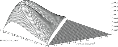
Figure 8. Phytoplankton bloom formation: (a) measurements adapted from Figure 2 in [Citation23] and (b) model results with accelerated coagulation.
![Figure 8. Phytoplankton bloom formation: (a) measurements adapted from Figure 2 in [Citation23] and (b) model results with accelerated coagulation.](/cms/asset/8f9cbe02-71e8-436c-9f3a-c00f741f945c/gipe_a_1310856_f0008_oc.gif)
Figure 9. Nutrient model performance with accelerated coagulation.
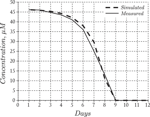
Figure 10. Phytoplankton bloom formation with accelerated coagulation: (a) error levels given by and (b) incremental total particle comparison.
The results (Figures and ) suggest that increasing the coagulation rate of small particles slightly improves the late-stage performance of the particle histogram model for particles between 0.4 and 1.0
without compromising the performance of the nutrient model (Figure ). However, accelerated coagulation rates increase the reproduction factor in this model by an order of magnitude (
) which leads to a uniform overestimation of the total particles (Figure ). These results further suggest that the reproduction process and hence the late stage particle dynamics could be modeled more accurately in the future by including the fragmentation process. Ample research exists investigating the role of the fragmentation process on size-structured aggregating particle systems, and parameter estimation within an inverse problem framework. Moreover, the techniques developed and insights presented by the researchers in [Citation53–Citation59] can be employed to include a fragmentation process explicitly which should improve the phytoplankton model predictions presented here.
8. Conclusions
This paper presents a new finite difference scheme (Equation4.1(4.1)
(4.1) ) for the size-structured particle aggregation problem (Equation2.1
(2.1)
(2.1) ) in the context of phytoplankton dynamics. The model includes growth and coagulation terms and a general system of differential equations which represent the environment. We prove that the numerical scheme (Equation4.1
(4.1)
(4.1) ) converges to the unique weak solution of the model (Equation2.1
(2.1)
(2.1) ). We then use the model to investigate the role of the aggregate growth processes on the formation of an algal bloom based on digitized measurements collected in the 1993 SIGMA reactor experiment [Citation23,Citation49]. The model simulations suggest that the aggregate growth rate processes (i.e. reproduction, encapsulation, growth rate of smallest aggregates) have an appreciable effect on the timing of nutrient depletion and bloom peak predictions.
The determination of a biologically sound mathematical expression for cell aggregate growth rates is confounded by the general assumption that only a portion of the aggregate is alive (i.e. active fraction) and capable of growth and cell division at any given time [Citation25]. We also note that the mathematical model of growth presented here and in many applications is based on the simplification that the aggregate particles can be represented using the concept of equivalent spherical diameter (ESD) determined by a volume balance. Real flocculated particles are irregular and more accurately characterized using fractal geometry techniques [Citation60]. The fractal properties of aggregates could affect physical (e.g. settling velocity) and biological characteristics (e.g. active volume, reproduction). These challenges are magnified when coupled with the notion of a variable internal storage pool which controls nutrient depletion rates. Moreover, nutrient uptake by aggregates depends not only on the outward size of the particle but more directly on the internal storage pool which allows growth and cell reproduction to continue when nutrients fall below the limits of chemical detection [Citation61]. The implication here is that in order to improve the predictions of algae bloom development and nutrient uptake, in addition to the environment and floc characteristics, there are at least three fundamental mechanisms requiring further investigation. We believe that the first mechanism is distributed reproduction, i.e. fragmentation which could serve to distribute particles more evenly across the size classes during the bloom peak. The second is the nutrient adsorption rate (e.g. as modeled by the Langmuir isotherm) which serves to pull nutrients into cell storage, and should depend on the active volume of the aggregate. The next (and perhaps more difficult) mechanism is the internal storage pool of cell aggregates and the rate at which nutrients are incorporated into the construction of new cell material (i.e. cell growth) [Citation62]. The rigorous development and application of an internal pool model (e.g. [Citation63]) including the adsorption and incorporation mechanisms in the more general context of cell aggregates should improve the performance of the model in biogeochemical applications.
Additional information
Funding
Notes
No potential conflict of interest was reported by the authors.
Related Research Data
References
- Banse K . Comment: does iron really limit phytoplankton production in the offshore subarctic Pacific? Limnol Oceanogr. 1990;35(3):772–775.
- Gregg WW , Ginoux P , Schopf PS , et al . Phytoplankton and iron: validation of a global three-dimensional ocean biogeochemical model. Deep Sea Res II. 2003;50:3143–3169.
- Jackson GA , Waite AM , Boyd PW . Role of algal aggregation in vertical carbon export during SOIREE and in other low biomass environments. Geophys Res Lett. 2005;32:1–4.
- Martin JH , Gordon RM , Fitzwater SE . The case for iron. Limnol Oceanogr. 1991;36(8):1793–1802.
- Miller CB , Frost BW , Booth BB , et al . Ecological processes in the subarctic Pacific: iron limitation cannot be the whole story. Oceanography. 1991;4(2):71–78.
- Mills MM , Ridame C , Davey M , et al . Iron and phosphorous co-limit nitrogen fixation in the eastern tropical North Atlantic. Nature. 2004;429:292–294.
- Sunda W , Huntsman SA . Interrelated influence of iron, light and cell size on marine phytoplankton growth. Nature. 1997;390:389–392.
- Timmermans KR , Gerringa LJA , de Baar HJW , et al . Growth rates of large and small Southern Ocean diatoms in relation to availability of iron in natural seawater. Limnol Oceanogr. 2001;46(2):260–266.
- Laurenceau-Cornec EC , Trull TW , Davies DM , et al . The relative importance of phytoplankton aggregates and zooplankton fecal pellets to carbon export: insights from free-drifting sediment trap deployments in naturally iron-fertilised waters near the Kergeulen Plateau. Biogeosciences. 2015;12:1007–1027.
- Chakraborty S , Lohrenz S . Phytoplankton community structure in the river-influenced continental margin of the northern Gulf of Mexico. Mar Ecol Prog Ser. 2015;521:31–47.
- Penta B , Ko D , Gould R , et al. Using coupled models to study the effects of river discharge on biogeochemical cycling and hypoxia in the northern Gulf of Mexico. Proceedings of the Oceans ‘09 MTS/IEEE Conference; Biloxi. 2009.
- North RL , Guildford SJ , Smith REH , et al . Evidence for phosphorous, nitrogen, and iron colimitation of phytoplankton communities in Lake Erie. Limnol Oceanogr. 2007;52(1):315–328.
- Takeda S , Tsuda A . An in situ iron-enrichment experiment in the western subarctic Pacific (SEEDS): introduction and summary. Prog Oceanogr. 2005;64:95–109.
- Banse K . Rates of phytoplankton cell division in the field iron enrichment experiments. Limnol Oceanogr. 1991;36(8):1886–1898.
- Bhattacharjee M , Siemann E . Low algal diversity systems are a promising method for biodiesel production in wastewater fed open reactors. Algae. 2015;30(1):67–79.
- Hannon M , Gimpel J , Tran M , et al . Biofuels from algae: challenges and potential. Biofuels. 2010;1(5):763–784.
- Hinckley S , Coyle KO , Gibson G , et al . A biophysical NPZ model with iron for the Gulf of Alaska: reproducing the differences between an oceanic HNLC ecosystem and a classical northern temperate shelf ecosystem. Deep Sea Res II. 2009;56:2520–2536.
- Huesemann MH , Van Wagenen J , Miller T , et al . A screening model to predict microalgae biomass growth in photobioreactors and raceway ponds. Biotechnol Bioeng. 2013;110:1583–1594.
- Kunjapur AM , Eldridge RB . Photobioreactor design for commercial biofuel production from microalgae. Ind Eng Chem Res. 2010;49:3516–3526.
- Milledge JJ , Heaven S . A review of the harvesting of micro-algae for biofuel production. Rev Environ Sci Biotechnol. 2012;12:165–178.
- Quinn JC , Yates T , Douglas N , et al . Nannochloropsis production metrics in a scalable outdoor photobioreactor for commercial applications. Biores Tech. 2012;117:164–171.
- Ackleh AS , Ferdinand R . A nonlinear phytoplankton aggregation model with light shading. SIAM J Appl Math. 1999;60:316–336.
- Ackleh AS , Hallam TG , Muller-Landau HC . Estimation of sticking and contact efficiencies in aggregation of phytoplankton: The SIGMA reactor experiment. Deep Sea Res. 1993;60(1995):185–201.
- Ackleh AS , Hallam TG , Smith WO Jr . Influences of aggregation and grazing on phytoplankton dynamics and fluxes: an individual-based modeling approach. Nonlinear World. 1994;1:473–492.
- Ackleh AS , Fitzpatrick BG . Modeling aggregation and growth processes in an algal population model: analysis and computations. J Math Biol. 1997;35:480–502.
- Jackson GA , Kiørboe T . Maximum phytoplankton concentrations in the sea. Limnol Oceanogr. 2008;53(1):395–399.
- Jackson GA , Lochmann SE . Effect of coagulation on nutrient and light limitation of an algal bloom. Limnol Oceanogr. 1992;37(1):77–89.
- Kiørboe T . Small-scale turbulence, marine snow formation, and planktivorous feeding. Sci Mar. 1997;61(Supl.1):141–158.
- Riebesell U . Particle aggregation during a diatom bloom. Mar Ecol Prog Ser. 1991;69:281–291.
- Arino O , Rudnicki R . Phytoplankton dynamics. C R Biol. 2004;327:961–969.
- Banasiak J , Noutchie S , Rudnicki R . Global solvability of a fragmentation-coagulation equation with growth and restricted coagulation. J Nonlinear Math Phys. 2009;16(1):13–26.
- Banasiak J , Lamb W . Coagulation, fragmentation and growth processes in a size structured population. Discret Contin Dyn Syst -- Ser B. 2009;11(3):563–585.
- Noutchie SC . Analysis of the effects of fragmentation-coagulation in planktology. C R Biol. 2010;333:789–792.
- Arrigo K . Marine microorganisms and global nutrient cycles. Nature. 2005;437:349–355.
- Xue Z , He R , Fennel K , et al . Modeling ocean circulation and biogeochemical variability in the Gulf of Mexico. Biogeosciences. 2013;10:7219–7234.
- Yu L , Fennel K , Laurent A , Murrell MC , Lehrter JC . Numerical analysis of the primary processes controlling oxygen dynamics on the Louisiana shelf. Biogeosciences. 2015;12:2063–2076.
- Zhao Y , Quigg A . Nutrient limitation in Northern Gulf of Mexico (NGOM): phytoplankton communities and photosynthesis respond to nutrient pulse. PLoS One. 2014;2(9):e88732. DOI:10.1371/journal.pone.0088732.
- Bortz DM , Jackson TL , Taylor KA , et al . Klebsiella pneumonia flocculation dynamics. Bull Math Biol. 2008;70(3):745–768.
- Brandt BW , Kooijman SALM . Two parameters account for the flocculated growth of microbes in biodegradation assays. Biotechnol Bioeng. 2000;70(6):677–684.
- Fredrickson AG . Population balance equations for cell and microbial cultures revisited. AIChE J. 2003;49(4):1050–1059.
- Smoller J . Shock waves and reaction-diffusion equations. 2nd ed. New York (NY): Springer-Verlag; 1994.
- Melzak ZA . The effect of coalescence in certain collision processes. Q Appl Math. 1953;11(2):231–234.
- Melzak ZA . A scalar transport equation. Trans Am Math Soc. 1957;85(2):547–560.
- Smoluchowski PM . Versuch einer mathematischen Theorie der Koagulationskinetik kolloider Lösungen. Physik Z. 1916;17:557–571 and 587--599.
- Farley K , Morel FM . Role of coagulation in the kinetics of sedimentation. Environ Sci Technol. 1986;20:187–195.
- Sinko JW , Streifer W . A new model for age-size structure of a population. Ecology. 1967;48:910–918.
- Filbet F , Laurençot P . Numerical simulation of the smoluchowski coagulation equation. SIAM J Sci Comput. 2004;25(6):2004–2028.
- Ackleh AS , Ma B , Miller R . A general nonlinear model for the interaction of a size-structured population and its environment: well-posedness and approximation. Q Appl Math. 2016;74:671–704.
- Alldredge AL , Gotschalk C , Passow U , et al . Mass aggregation of diatom blooms: insights from a mesocosm study. Deep Sea Res II. 1995;42(1):9–27.
- Banks HT , Catenacci J , Hu S . Use of difference-based methods to explore statistical and mathematical model discrepancy in inverse problems. J Inverse Ill-Posed Prob. 2016;24:413–433.
- Cintron-Arias A , Banks HT , Capaldi A , et al . A sensitivity matrix based methodology for inverse problem formulation. J Inverse Ill-Posed Prob. 2009;17(6):545–564.
- Martins JRRA , Strudza P , Alonso JJ . The complex-step derivative approximation. ACM T Math Soft. 2003;29(3):245–262.
- Ackleh AS . Parameter estimation in a structured algal coagulation-fragmentation model. Nonlinear Anal. Theory Methods Appl. 1997;28(5):837–854.
- Bache D . Floc rupture and turbulence: A framework for analysis. Chem Eng Sci. 2004;59(12):2521–2534.
- Byrne E , Dzul S , Solomon M , et al . Postfragmentation density function for bacterial aggregates in laminar flow. Phys Rev E. 2011;83(4): 041911.
- Doumic M , Tine LM . Estimating the division rate for the growth-fragmentation equation. J Math Biol. 2012;67(1):69–103.
- Liu J , Zhou M , Zhou J , et al. Derivation and verification of the breakage rate coefficient during flocculation process based on shear strength. In: Kao JCM , Sung WP , and Chen R , editors. Materials, transportation and environmental engineering, Pts 1 and 2. Vols. 779--780, Stafa-Zurich: Trans Tech Publications Ltd; 2013. p. 1482–1489. WOS:000336106300288.
- Mirzaev I , Byrne EC , Bortz DM . An inverse problem for a class of conditional probability measure-dependent evolution equations. Inverse Prob. 2016;32(9):0950005.
- Ziff RM , McGrady ED . The kinetics of cluster fragmentation and depolymerisation. J Phys A: Math Gen. 1985;18(15):3027–3037.
- Arasan S , Akbulut S , Hasiloglu AS . The relationship between the fractal dimension and shape properties of particles. KSCE J Civ Eng. 2011;15(7):1219–1225.
- Droop MR . Comment: in defence of the cell quota model of micro-algal growth. J Plankton Res. 2003;25(1):103–107.
- Buitenhuis ET , Geider RJ . A model of phytoplankton acclimation to iron-light colimitation. Limnol Oceanogr. 2010;55(2):714–724.
- Pahlow M , Oschlies A . Optimal allocation backs Droop’s cell-quota model. Mar Ecol Prog Ser. 2013;473:1–5.
- Brauer F , Noel J . The qualitative theory of ordinary differential equations. New York (NY): Dover; 1989.
Appendix 1
Proofs of lemmas and theorems
Proof of Lemma 4.1:
First observe that for any real numbers and positive integer N we have the interchange of summation
so by direct calculation and assumption (B10),
where the last step follows from assumption (B10), namely if
. Therefore,
(A1)
(A1)
This completes the proof.
Proof of Lemma 4.2:
First multiply the first row of (Equation4.1(4.1)
(4.1) ) by
and sum from
to N to get
(A2)
(A2)
which follows from assumption (B1), Lemma 4.1, and nonnegativity of the numerical scheme, respectively. Since the scheme is nonnegative, we have and hence by (EquationA1
(A1)
(A1) ), noting that
the relationship (EquationA2
(A2)
(A2) ) satisfies
Next observe that by nonnegativity of the scheme and (B3) and (B4),
By nonnegativity of we have
and since
, we get
Thus,
Let ,
, and
.
(A3)
(A3)
The result now follows from inductive application of (EquationA3(A3)
(A3) ) and elementary calculations.
Proof of Lemma 4.3:
Define
If , substituting the boundary conditions at the corner, and appealing to assumptions (B6), (B7), and Lemma 4.2,
Otherwise, fix , and multiply the numerical scheme by
,
(A4)
(A4)
Using , nonnegativity of the scheme, and
we have
Let , and by assumption (B5) we arrive at
By induction on k and assumption (B9) we establish the upper bound .
Proof of Lemma 4.4:
We omit the details for the constant , since the results follow directly from Lemma 4.2 and the arguments presented in Lemma 5.3 in [Citation48]. Observe that by (Equation4.1
(4.1)
(4.1) ),
and,
and hence by assumption (B2) and Lemmas 4.2 and 4.3,
Next observe that by the boundary condition in (Equation4.1(4.1)
(4.1) ), we have
(A5)
(A5)
Next observe that
from which we obtain,
Let and from Lemmas 4.1 through 4.3 and previous results established in this Lemma we obtain
By (EquationA5(A5)
(A5) ) we have
This completes the proof.
Proof of Lemma 4.5:
From the first row of (Equation4.1(4.1)
(4.1) ), we obtain
Applying the triangle inequality, nonnegativity of the numerical scheme, and assumptions (B1) and (B2), we have
Noting that , then summing from
to
,
By Lemmas 4.1 and 4.4,
By assumption (B2), Lemmas 4.2 and 4.3,(A6)
(A6)
Adding to both sides of (EquationA6
(A6)
(A6) ) we obtain
By Lemma 4.4,
where . Let
to arrive at the following recurrence relationship,
(A7)
(A7)
The constant is established using a standard induction argument on (EquationA7
(A7)
(A7) ).
Proof of Lemma 4.6:
Multiplying the first row in the numerical scheme (Equation4.1(4.1)
(4.1) ) by
we obtain
Applying the triangle inequality, summing from , and applying Lemma 4.4,
(A8)
(A8)
It clearly follows that
and by Lemma 4.4,
Let to complete the proof.
Proof of Theorem 5.1:
The result for the population density u can be established using similar techniques as in the proof of Lemma 16.10 (p.279) in [Citation41]. By Lemma 4.6 each component () in the sequence
approximating the environment satisfies a Lipschitz condition on [0, T] and by the assumptions on
and
, each component of the approximating sequence defines a bounded equi-Lipschitz family. Thus the family
is equicontinuous and by the Arzela–Ascoli Theorem one can extract a uniformly convergent subsequence in C[0, T].
Proof of Theorem 5.2:
First observe that convergence of a sequence in C[0, T] is uniform convergence. Applying the Picard Iteration to the limit function
as outlined in [Citation64], (Pgs 112-127) we can show that
is a weak solution to our ODE system. So it suffices to establish the weak solution result for u. Let
and denote the values of
on the numerical mesh
by
. Multiplying the first equation of the difference scheme (Equation4.1
(4.1)
(4.1) ) by
, and adding and subtracting several terms:
Multiplying by and
and summing from
, and
, evaluating the telescoping sums, noting that
, and inserting the corner boundary condition we have
(A9)
(A9)
Using similar techniques as in the proof of Lemma 16.10 in [Citation41] (p.279) we can show that the above Equation (EquationA9(A9)
(A9) ) converges (as
) to Equation (3.1) for any convergent subsequence defined in Theorem 5.1. The
,
and BV bounds on u follow by observing that
convergence obtained in Theorem 5.1 implies pointwise convergence almost everywhere (along a subsequence) and then taking limits in the estimates established in Lemmas 4.2, 4.3 and 4.5.
Proof of Lemma 5.3:
We let , and observe that
satisfies
(A10)
(A10)
Multiplying both sides of (EquationA10(A10)
(A10) ) by
we obtain
Applying the triangle inequality and nonnegativity of the parameters ,
, and the numerical scheme
we obtain,
Applying nonnegativity on the parameters and summing from to N,
For convenience, let . Applying the triangle inequality and the Lipschitz conditions on the model parameters we obtain,
Evaluating the telescoping sum on the left hand side,(A11)
(A11)
Note that,
and the triangle inequality yields,
Define the following constants: ,
,
. By (EquationA11
(A11)
(A11) ) and assumption (B1) we have
(A12)
(A12)
Observe also that by the fifth row in (Equation4.1(4.1)
(4.1) ) we have,
Letting ,
and summing from
,
(A13)
(A13)
From (EquationA12(A12)
(A12) ) and (EquationA13
(A13)
(A13) ) we obtain,
(A14)
(A14)
By the triangle inequality and assumption (B8) on and
, we obtain
and that
. As a result, there exists a constant
such that
(A15)
(A15)
Applying a standard induction argument on k we arrive at
Let to complete the proof.