Identification of diffusion parameters in a non-linear convection–diffusion equation using adaptive homotopy perturbation method

Abstract

This paper is concerned with the numerical identification of diffusion parameters in a non-linear convection–diffusion equation, which arises as the saturation equation in the fractional flow formulation of the two-phase porous media flow equations. In order to overcome the defect of the local convergence of traditional methods, an adaptive homotopy perturbation method is applied to solve this parameter identification inverse problem. The adaptive homotopy perturbation method provides a simple way to adapt computational refinement to the choice of the homotopy parameter. Numerical simulations illustrate that the proposed algorithm is globally convergent and computationallyefficient.

Keywords:

• Inverse problems
• non-linear convection–diffusion equation
• homotopy perturbation method
• Tikhonov regularization
• porous media flow

AMS Subject Classifications:

• 35R30
• 65H20
• 65M32
• 76S05

1. Introduction

This article studies the numerical solution to the following inverse problem. That is to find the unknown diffusion coefficient $q(\mathbf{x})$ which satisfies the following two-dimensional non-linear convection–diffusion equation:(1.1) $$\begin{array}{c}\hfill u_t+\frac{\mathit{\partial }}{\mathit{\partial }x}f(u)+\frac{\mathit{\partial }}{\mathit{\partial }y}g(u)-\mathrm{\nabla }·(q(\mathbf{x})N(u)\mathrm{\nabla }u)=s(\mathbf{x},t),(\mathbf{x},t)\in \mathrm{\Omega }\times (0,T),\end{array}$$(1.1)

with the initial-boundary conditions(1.2) $$\begin{array}{c}\hfill u(\mathbf{x},0)=u_0(\mathbf{x}),\mathbf{x}\in \mathrm{\Omega },\end{array}$$(1.2) (1.3) $$\begin{array}{c}\hfill u(\mathbf{x},t)=0,(\mathbf{x},t)\in \mathit{\partial }\mathrm{\Omega }\times (0,T),\end{array}$$(1.3)

subject to the observed data(1.4) $$\begin{array}{c}\hfill u({\mathbf{x}}^d,t)=k({\mathbf{x}}^d,t),d=1,2,\dots ,D,t\in (0,T),\end{array}$$(1.4)

where f and g are S-shaped flux functions of Buckley–Leverett type in the x- and y-direction, respectively, N is a positive non-linear function of u, and s is the piecewise smooth source function. For simplicity, $\mathrm{\Omega }$ is assumed to be the unit square, and the flux term is written in the following form$$\mathrm{\nabla }·(f,g)=\frac{\mathit{\partial }}{\mathit{\partial }x}f(u)+\frac{\mathit{\partial }}{\mathit{\partial }y}g(u).$$

Equation (1.1(1.1) $$\begin{array}{c}\hfill u_t+\frac{\mathit{\partial }}{\mathit{\partial }x}f(u)+\frac{\mathit{\partial }}{\mathit{\partial }y}g(u)-\mathrm{\nabla }·(q(\mathbf{x})N(u)\mathrm{\nabla }u)=s(\mathbf{x},t),(\mathbf{x},t)\in \mathrm{\Omega }\times (0,T),\end{array}$$(1.1) ) is closely relevant to two-phase porous media flow. The system of partial differential equations modelling the immiscible displacement of oil by water in a porous media with zero gravity effects is (see [1])(1.5) $$\begin{array}{cc}& \mathit{\varphi }(\mathbf{x})u_t+\mathrm{\nabla }·(f(u)\mathbf{V}+f_g(u)q(\mathbf{x})\mathrm{\nabla }h)-\mathrm{\nabla }·(q(\mathbf{x})N(u)\mathrm{\nabla }u)=f_1(\mathbf{x},t),\hfill \end{array}$$(1.5) (1.6) $$\begin{array}{cc}& \mathrm{\nabla }·\mathbf{V}=f_2(\mathbf{x},t),\hfill \end{array}$$(1.6) (1.7) $$\begin{array}{cc}& \mathbf{V}=-q(\mathbf{x})\mathit{\lambda }(\mathbf{x},u)(\mathrm{\nabla }\overline{p}-\mathit{\rho }(u)\mathrm{\nabla }h),\hfill \end{array}$$(1.7) (1.8) $$\begin{array}{cc}& f_g(u)=(\mathit{\rho }(u)-{\mathit{\rho }}_0(u))f(u){\mathit{\lambda }}_0(\mathbf{x},u).\hfill \end{array}$$(1.8)

Here, $f_1$ and $f_2$ are, respectively, the production and injection wells, $\mathit{\rho }$ and ${\mathit{\rho }}_0$ are, respectively, the densities of the wetting and non-wetting phases, $\mathit{\varphi }$ is the porosity, $\mathbf{V}$ is the total Darcy velocity, q is the permeability, h is the height, $\overline{p}$ is the global pressure, u is the saturation of the wetting phase, $\mathit{\lambda }$ is the total mobility of the phases and ${\mathit{\lambda }}_0$ is the phase mobility of the non-wetting phase. N is a non-linear diffusion function, and f is an S-shaped non-linear fractional flow function.

Equation (1.1(1.1) $$\begin{array}{c}\hfill u_t+\frac{\mathit{\partial }}{\mathit{\partial }x}f(u)+\frac{\mathit{\partial }}{\mathit{\partial }y}g(u)-\mathrm{\nabla }·(q(\mathbf{x})N(u)\mathrm{\nabla }u)=s(\mathbf{x},t),(\mathbf{x},t)\in \mathrm{\Omega }\times (0,T),\end{array}$$(1.1) ) is similar to Equation (1.5(1.5) $$\begin{array}{cc}& \mathit{\varphi }(\mathbf{x})u_t+\mathrm{\nabla }·(f(u)\mathbf{V}+f_g(u)q(\mathbf{x})\mathrm{\nabla }h)-\mathrm{\nabla }·(q(\mathbf{x})N(u)\mathrm{\nabla }u)=f_1(\mathbf{x},t),\hfill \end{array}$$(1.5) ), except for the time derivative term and the convection term. The time derivative terms in Equations (1.1(1.1) $$\begin{array}{c}\hfill u_t+\frac{\mathit{\partial }}{\mathit{\partial }x}f(u)+\frac{\mathit{\partial }}{\mathit{\partial }y}g(u)-\mathrm{\nabla }·(q(\mathbf{x})N(u)\mathrm{\nabla }u)=s(\mathbf{x},t),(\mathbf{x},t)\in \mathrm{\Omega }\times (0,T),\end{array}$$(1.1) ) and (1.5(1.5) $$\begin{array}{cc}& \mathit{\varphi }(\mathbf{x})u_t+\mathrm{\nabla }·(f(u)\mathbf{V}+f_g(u)q(\mathbf{x})\mathrm{\nabla }h)-\mathrm{\nabla }·(q(\mathbf{x})N(u)\mathrm{\nabla }u)=f_1(\mathbf{x},t),\hfill \end{array}$$(1.5) ) will be equal if $\mathit{\varphi }(\mathbf{x})=1$. The difference in the convection terms between Equations (1.1(1.1) $$\begin{array}{c}\hfill u_t+\frac{\mathit{\partial }}{\mathit{\partial }x}f(u)+\frac{\mathit{\partial }}{\mathit{\partial }y}g(u)-\mathrm{\nabla }·(q(\mathbf{x})N(u)\mathrm{\nabla }u)=s(\mathbf{x},t),(\mathbf{x},t)\in \mathrm{\Omega }\times (0,T),\end{array}$$(1.1) ) and (1.5(1.5) $$\begin{array}{cc}& \mathit{\varphi }(\mathbf{x})u_t+\mathrm{\nabla }·(f(u)\mathbf{V}+f_g(u)q(\mathbf{x})\mathrm{\nabla }h)-\mathrm{\nabla }·(q(\mathbf{x})N(u)\mathrm{\nabla }u)=f_1(\mathbf{x},t),\hfill \end{array}$$(1.5) ) is only that the convection term in Equation (1.1(1.1) $$\begin{array}{c}\hfill u_t+\frac{\mathit{\partial }}{\mathit{\partial }x}f(u)+\frac{\mathit{\partial }}{\mathit{\partial }y}g(u)-\mathrm{\nabla }·(q(\mathbf{x})N(u)\mathrm{\nabla }u)=s(\mathbf{x},t),(\mathbf{x},t)\in \mathrm{\Omega }\times (0,T),\end{array}$$(1.1) ) does not have permeability dependence and varying coefficient.

Oil reservoir simulation based on the parameter identification problem of non-linear convection–diffusion Equation (1.1(1.1) $$\begin{array}{c}\hfill u_t+\frac{\mathit{\partial }}{\mathit{\partial }x}f(u)+\frac{\mathit{\partial }}{\mathit{\partial }y}g(u)-\mathrm{\nabla }·(q(\mathbf{x})N(u)\mathrm{\nabla }u)=s(\mathbf{x},t),(\mathbf{x},t)\in \mathrm{\Omega }\times (0,T),\end{array}$$(1.1) ) is a powerful tool to help make important decisions in areas such as oil and gas exploration, management of petroleum reservoirs, etc. With its help, researchers can easily select, for example, the type of recovery method, fluid production rate, fluid injection rate and well location. In general, this parameter identification problem is computationally hard to solve. First, the conventional methods such as the quasi-Newton or Gauss–Newton are locally convergent. When there is no prior information available, the initial guess is usually chosen to be a constant. In oil reservoirs where the parameter often has large jumps, the conventional methods may diverge when the initial guess is chosen as an arbitrary constant. So these conventional methods are not always successful in real applications. Second, the identification requires an exuberant number of calls to the forward simulator in order to achieve convergence, and the direct model is described by the solution of the non-linear convection–diffusion equation which is computationally demanding to solve. Therefore, the identification needs a large amount of calculation. As stated above, there will be an urgent need for a parameter identification method able to overcome these two issues. The aim of this paper is to further develop such parameter identification methods.

There are many articles [2–6] focusing on the development of appropriate methods for recovery of $q(\mathbf{x})$ within the linear elliptic equation(1.9) $$\begin{array}{c}\hfill -\mathrm{\nabla }·(q(\mathbf{x})\mathrm{\nabla }u)=s(\mathbf{x}).\end{array}$$(1.9)

Less work [7–10] has been done on the identification of $q(\mathbf{x})$ in the linear parabolic equation(1.10) $$\begin{array}{c}\hfill u_t-\mathrm{\nabla }·(q(\mathbf{x})\mathrm{\nabla }u)=s(\mathbf{x},t).\end{array}$$(1.10)

Equations (1.9(1.9) $$\begin{array}{c}\hfill -\mathrm{\nabla }·(q(\mathbf{x})\mathrm{\nabla }u)=s(\mathbf{x}).\end{array}$$(1.9) )–(1.10(1.10) $$\begin{array}{c}\hfill u_t-\mathrm{\nabla }·(q(\mathbf{x})\mathrm{\nabla }u)=s(\mathbf{x},t).\end{array}$$(1.10) ) can be considered as the descriptions of one-phase flow processes in porous media where $q(\mathbf{x})$ is the permeability. For the permeability identification problems in the practical application, the interested readers are invited to refer to, e.g. [11–14].

In the last two decades, perturbation methods, which are based on a small parameter involved in the equation, have been widely used by researchers to solve non-linear problems. An appropriate choice of small parameters can give good results; on the contrary, unsuitable choice of small parameters often leads to bad results. In order to eliminate the limitations of the traditional perturbation techniques, he [15–17] proposed homotopy perturbation method by combining the traditional perturbation technique with the homotopy method. He successfully applied homotopy perturbation method to solve non-linear oscillators with discontinuities [18], non-linear wave equations [19], and compared this method with homotopy analysis method [20]. Li et al. [21] applied homotopy perturbation methods to a time-fractional diffusion equation with a moving boundary condition, and Mohyud-Din and Yildirim [22] used homotopy perturbation approach to solve homogeneous and inhomogeneous advection problems. Nilssen et al. [23] applied homotopy perturbation method to a moving boundary problem involving space-time fractional derivative, and Rajeev [24] developed homotopy perturbation approach for a Stefan problem with variable latent heat. More recently, homotopy perturbation methods have also been investigated to solve inverse problems, such as inverse heat conduction problems [25–27], inverse Stefan problems [28,29] and inverse diffusion problem [30].

The objective of this paper is to develop an adaptive homotopy perturbation method for solving the permeability identification problem of a non-linear convection–diffusion equation. A homotopy perturbation technique for this inverse problem is first studied, and then extended to adaptively choose the homotopy parameters. In this way, the computational refinements are adapted to the choice of the homotopy parameters at which the algorithm can effectively reduce the cost, and thus improve computational efficiency. This adaptive homotopy perturbation method turns out to be globally convergent, computationally efficient and stable with respect to noise.

The remainder of this paper is organized as follows. In Section 2, the numerical scheme that is used to discretize the forward problem is presented. In Section 3, the proposed adaptive homotopy perturbation method in detail is presented. Simulation examples are given in Section 4. Finally, the conclusion remarks are presented in Section 5.

2. Finite-difference discretization

We can discretize Equation (1.1(1.1) $$\begin{array}{c}\hfill u_t+\frac{\mathit{\partial }}{\mathit{\partial }x}f(u)+\frac{\mathit{\partial }}{\mathit{\partial }y}g(u)-\mathrm{\nabla }·(q(\mathbf{x})N(u)\mathrm{\nabla }u)=s(\mathbf{x},t),(\mathbf{x},t)\in \mathrm{\Omega }\times (0,T),\end{array}$$(1.1) ) by a finite difference equation as follows:(2.1) $$\begin{array}{cc}& \frac{u_{i,j}^n-u_{i,j}^{n-1}}{\mathrm{\Delta }t}+\mathrm{\nabla }·(f(u_{i,j}^{n-1}),g(u_{i,j}^{n-1}))-\mathrm{\nabla }·(q_{i,j}{N}_{i,j}^n\mathrm{\nabla }{u}_{i,j}^n)=s_{i,j}^n,\hfill \\ \hfill & n=1,2,\dots ,M;i=1,2,\dots ,n_1-1;j=1,2,\dots ,n_2-1,\hfill \end{array}$$(2.1)

where$$\begin{array}{cc}\hfill u_{i,j}^n& =u(i\mathrm{\Delta }x,j\mathrm{\Delta }y,n\mathrm{\Delta }t),s_{i,j}^n=s(i\mathrm{\Delta }x,j\mathrm{\Delta }y,n\mathrm{\Delta }t),q_{i,j}=q(i\mathrm{\Delta }x,j\mathrm{\Delta }y),\hfill \\ \hfill N_{i,j}^n& =N(u_{i,j}^n),n_1=\frac{1}{\mathrm{\Delta }x},n_2=\frac{1}{\mathrm{\Delta }y},M=\frac{T}{\mathrm{\Delta }t},\hfill \end{array}$$$\mathrm{\Delta }x$ and $\mathrm{\Delta }y$ are the step sizes of the rectangular grid in the x- and y-direction, respectively, and $\mathrm{\Delta }t$ is the time step size. $\mathrm{\nabla }·(q_{i,j}{N}_{i,j}^n\mathrm{\nabla }{u}_{i,j}^n)$ and $\mathrm{\nabla }·(f(u_{i,j}^{n-1}),g(u_{i,j}^{n-1}))$ are, respectively, the discretizations of the diffusion term and the convection term, and to obtain their expressions, the following definitions are given.

The discrete derivatives in the x-direction are denoted as$$D_{-}^x{u}_{i,j}^n=\frac{u_{i,j}^n-u_{i-1,j}^n}{\mathrm{\Delta }x},D_{+}^x{u}_{i,j}^n=\frac{u_{i+1,j}^n-u_{i,j}^n}{\mathrm{\Delta }x}$$

for the backward and forward difference approximations, respectively. For the discrete derivatives in the y-direction, a corresponding notation is used.

The mean values for the discretized permeability q are defined as$${\overline{q}}_{i,j+\frac{1}{2}}^x=\frac{1}{2}(q_{i+\frac{1}{2},j+\frac{1}{2}}+q_{i-\frac{1}{2},j+\frac{1}{2}}),{\overline{q}}_{i+\frac{1}{2},j}^y=\frac{1}{2}(q_{i+\frac{1}{2},j+\frac{1}{2}}+q_{i+\frac{1}{2},j-\frac{1}{2}}),$$

where $q_{i+\frac{1}{2},j+\frac{1}{2}}=q((i+\frac{1}{2})\mathrm{\Delta }x,(j+\frac{1}{2})\mathrm{\Delta }y)$. The mean values for the non-linear function N(u) are defined as$${\left({\overline{N}}^x\right)}_{i+\frac{1}{2},j}^n=\frac{1}{2}\left(N_{i+1,j}^n+N_{i,j}^n\right),{\left({\overline{N}}^y\right)}_{i,j+\frac{1}{2}}^n=\frac{1}{2}\left(N_{i,j+1}^n+N_{i,j}^n\right).$$

Then, the discretization of the diffusion term is expressed as$$\mathrm{\nabla }·(q_{i,j}{N}_{i,j}^n\mathrm{\nabla }{u}_{i,j}^n)=D_{-}^x\left({\overline{q}}_{i+\frac{1}{2},j}^y{\left({\overline{N}}^x\right)}_{i+\frac{1}{2},j}^n{D}_{+}^x{u}_{i,j}^n\right)+D_{-}^y\left({\overline{q}}_{i,j+\frac{1}{2}}^x{\left({\overline{N}}^y\right)}_{i,j+\frac{1}{2}}^n{D}_{+}^y{u}_{i,j}^n\right).$$

For the convection term, the Engquist–Osher upwind scheme is used (see [31])$$\mathrm{\nabla }·(f(u_{i,j}^{n-1}),g(u_{i,j}^{n-1}))=D_{-}^x{f}^{EO}\left(u_{i,j}^{n-1},u_{i+1,j}^{n-1}\right)+D_{-}^y{g}^{EO}\left(u_{i,j}^{n-1},u_{i,j+1}^{n-1}\right),$$

where the Engquist–Osher numerical flux functions $f^{EO}\left(u_{i,j}^{n-1},u_{i+1,j}^{n-1}\right)$ and $g^{EO}(u_{i,j}^{n-1},u_{i,j+1}^{n-1})$ are denoted as$$\begin{array}{cc}& f^{EO}\left(u_{i,j}^{n-1},u_{i+1,j}^{n-1}\right)=\frac{1}{2}\left(f\left(u_{i,j}^{n-1}\right)+f\left(u_{i+1,j}^{n-1}\right)\right)-\frac{1}{2}{\int }_{u_{i,j}^{n-1}}^{u_{i+1,j}^{n-1}}|f^{\prime }(\mathit{\xi })|\mathrm{d}\mathit{\xi },\hfill \\ \hfill & g^{EO}\left(u_{i,j}^{n-1},u_{i,j+1}^{n-1}\right)=\frac{1}{2}\left(g\left(u_{i,j}^{n-1}\right)+g\left(u_{i,j+1}^{n-1}\right)\right)-\frac{1}{2}{\int }_{u_{i,j}^{n-1}}^{u_{i,j+1}^{n-1}}|g^{\prime }(\mathit{\xi })|\mathrm{d}\mathit{\xi }.\hfill \end{array}$$

The explicit formulas for $f^{EO}$ and $g^{EO}$, for examples of f and g, are calculated in the Appendix 1.

The upwind scheme is a first-order scheme, which can solve convection-dominated problems. In [23], Nilssen et al. commented on the regularity with respect to the numerical solution u of the numerical flux functions. Notice that the convection term is defined explicitly in time, while the diffusion term is discretized implicitly, which is also similar to [23]. Such issues are not the theme of this paper, the interested reader is directed their article and references therein for more detailed information.

The initial-boundary conditions (1.2(1.2) $$\begin{array}{c}\hfill u(\mathbf{x},0)=u_0(\mathbf{x}),\mathbf{x}\in \mathrm{\Omega },\end{array}$$(1.2) ) and (1.3(1.3) $$\begin{array}{c}\hfill u(\mathbf{x},t)=0,(\mathbf{x},t)\in \mathit{\partial }\mathrm{\Omega }\times (0,T),\end{array}$$(1.3) ) are, respectively, discretized as(2.2) $$\begin{array}{c}\hfill u_{i,j}^0=u_0(i\mathrm{\Delta }x,j\mathrm{\Delta }y),i=0,1,\dots ,n_1;j=0,1,\dots ,n_2,\end{array}$$(2.2) (2.3) $$\begin{array}{c}\hfill \begin{array}{cc}& u_{0,j}^n=u_{n_1,j}^n=u_{i,0}^n=u_{i,n_2}^n=0,\hfill \\ \hfill & n=1,2,\dots ,M;i=0,1,\dots ,n_1;j=0,1,\dots ,n_2.\hfill \end{array}\end{array}$$(2.3)

Remark 2.1:

Due to the implicit treatment of the diffusion term, the system that needs to be solved for each time level in the forward simulation is non-linear. The Picard iteration is used to solve these resultant non-linear systems. If the non-linear system is written on the form $B(u)u=b$, where B(u) is a non-singular matrix depending non-linearly on u, then we iterate$$B(u^{k-1})u^k=b,$$

until convergence, with $u^0$ given. $u^0$ is usually the solution from the previous time level. If we let$$\begin{array}{cc}\hfill u^{\top }& =(u_{1,1}^n,u_{1,2}^n,\dots ,u_{1,n_2-1}^n,u_{2,1}^n,u_{2,2}^n,\dots ,u_{2,n_2-1}^n,\hfill \\ \hfill & \dots ,u_{n_1-1,1}^n,u_{n_1-1,2}^n,\dots ,u_{n_1-1,n_2-1}^n),\hfill \end{array}$$

then B is a block tridiagonal matrix. We can conveniently solve this block tridiagonal matrix equation with the chase method. This Picard iteration method is only used to solve the forward problem.

Remark 2.2:

We can see from the above method that the discretized permeability used in the forward simulation is $q_{i+\frac{1}{2},j+\frac{1}{2}}$, $i=0,1,\dots ,n_1-1$; $j=0,1,\dots ,n_2-1$. So the discretized permeability vector $q\in R^{n_1\times n_2}$ is needed. The initial grid and a coarse grid are, respectively, denoted as ${\mathrm{\Omega }}^{n_1\times n_2}$ and ${\mathrm{\Omega }}^{m_1\times m_2}$, where ${\mathrm{\Omega }}^{m_1\times m_2}$ is got by coarsening ${\mathrm{\Omega }}^{n_1\times n_2}$, $n_1\times n_2$ and $m_1\times m_2$ are, respectively, the grid numbers of the initial grid and the coarse grid. Similar to [23], $q\in R^{m_1\times m_2}$ is defined at ${\mathrm{\Omega }}^{m_1\times m_2}$, and a constant prolongation is used when $q\in R^{n_1\times n_2}$ is needed. The constant prolongation means that the entry of q at ${\mathrm{\Omega }}^{n_1\times n_2}$ is obtained by taking the value from the closed point of ${\mathrm{\Omega }}^{m_1\times m_2}$. As a matter of fact , $m_1\times m_2$ is generally dependent on the number of available measurements.

3. Adaptive homotopy perturbation method

In this section, we derive a specific adaptive homotopy perturbation method for the identification of diffusion parameters in the non-linear convection–diffusion equation. To deduce this method, we first describe the inversion model in a discrete setting and construct a basic iterative method in Section 3.1, and then begin at the general homotopy perturbation method in Section 3.2. In Section 3.3, the adaptive homotopy perturbation method is designed by adaptively choosing the homotopy parameters.

3.1. Inversion model and basic iterative method

Equation (1.4(1.4) $$\begin{array}{c}\hfill u({\mathbf{x}}^d,t)=k({\mathbf{x}}^d,t),d=1,2,\dots ,D,t\in (0,T),\end{array}$$(1.4) ) is discretized as(3.1) $$\begin{array}{c}\hfill u_{{\mathbf{x}}^d}^n=k_{{\mathbf{x}}^d}^n,n=1,2,\dots ,M;d=1,2,\dots ,D.\end{array}$$(3.1)

The difference Equations (2.1(2.1) $$\begin{array}{cc}& \frac{u_{i,j}^n-u_{i,j}^{n-1}}{\mathrm{\Delta }t}+\mathrm{\nabla }·(f(u_{i,j}^{n-1}),g(u_{i,j}^{n-1}))-\mathrm{\nabla }·(q_{i,j}{N}_{i,j}^n\mathrm{\nabla }{u}_{i,j}^n)=s_{i,j}^n,\hfill \\ \hfill & n=1,2,\dots ,M;i=1,2,\dots ,n_1-1;j=1,2,\dots ,n_2-1,\hfill \end{array}$$(2.1) ), (2.2(2.2) $$\begin{array}{c}\hfill u_{i,j}^0=u_0(i\mathrm{\Delta }x,j\mathrm{\Delta }y),i=0,1,\dots ,n_1;j=0,1,\dots ,n_2,\end{array}$$(2.2) ), (2.3(2.3) $$\begin{array}{c}\hfill \begin{array}{cc}& u_{0,j}^n=u_{n_1,j}^n=u_{i,0}^n=u_{i,n_2}^n=0,\hfill \\ \hfill & n=1,2,\dots ,M;i=0,1,\dots ,n_1;j=0,1,\dots ,n_2.\hfill \end{array}\end{array}$$(2.3) ) and (3.1(3.1) $$\begin{array}{c}\hfill u_{{\mathbf{x}}^d}^n=k_{{\mathbf{x}}^d}^n,n=1,2,\dots ,M;d=1,2,\dots ,D.\end{array}$$(3.1) ) define a non-linear operator equation $F(Q)=K$, where Q denotes a vector which is composed of $q_{i,j}$ in a suitable sequence, and K denotes a vector which is composed of $k_{{\mathbf{x}}^d}^n$ in a suitable sequence. Let ${\widehat{k}}_{{\mathbf{x}}^d}^n$ denote the observations and form the vector $\widehat{K}$ in the same sequence as K. Especially, let$$\begin{array}{cc}\hfill Q^{\top }& =(q_{1,1},q_{1,2},\dots ,q_{1,m_2},q_{2,1},q_{2,2},\dots ,q_{2,m_2},\dots ,q_{m_1,1},q_{m_1,2},\dots ,q_{m_1,m_2}),\hfill \\ \hfill K^{\top }& =(k_{{\mathbf{x}}^1}^1,k_{{\mathbf{x}}^2}^1,\dots ,k_{{\mathbf{x}}^D}^1,k_{{\mathbf{x}}^1}^2,k_{{\mathbf{x}}^2}^2,\dots ,k_{{\mathbf{x}}^D}^2,\dots ,k_{{\mathbf{x}}^1}^M,k_{{\mathbf{x}}^2}^M,\dots ,k_{{\mathbf{x}}^D}^M),\hfill \\ \hfill {\widehat{K}}^{\top }& =({\widehat{k}}_{{\mathbf{x}}^1}^1,{\widehat{k}}_{{\mathbf{x}}^2}^1,\dots ,{\widehat{k}}_{{\mathbf{x}}^D}^1,{\widehat{k}}_{{\mathbf{x}}^1}^2,{\widehat{k}}_{{\mathbf{x}}^2}^2,\dots ,{\widehat{k}}_{{\mathbf{x}}^D}^2,\dots ,{\widehat{k}}_{{\mathbf{x}}^1}^M,{\widehat{k}}_{{\mathbf{x}}^2}^M,\dots ,{\widehat{k}}_{{\mathbf{x}}^D}^M).\hfill \end{array}$$

Then, the problem of inversing Q is reduced to a non-linear operator equation(3.2) $$\begin{array}{c}\hfill F(Q)=\widehat{K}.\end{array}$$(3.2)

Tikhonov regularization of such an ill-posed problem is achieved by replacing the operator Equation (3.2(3.2) $$\begin{array}{c}\hfill F(Q)=\widehat{K}.\end{array}$$(3.2) ) by the optimal problem(3.3) $$\begin{array}{c}\hfill min\left\{\Vert F(Q)-\widehat{K}{\Vert }^2+{\mathit{\beta }}_1\Vert L_1(Q-Q^0){\Vert }^2+{\mathit{\beta }}_2{\Vert L_2(Q-Q^0)\Vert }^2\right\},\end{array}$$(3.3)

where $L_1$, $L_2$ are the second-order smooth matrices in the x- and y-direction, respectively (see [19]), and ${\mathit{\beta }}_1$, ${\mathit{\beta }}_2$ are the regularization parameters.

It is easy to see that the optimal solution $Q^{\ast }$ of Equation (3.3(3.3) $$\begin{array}{c}\hfill min\left\{\Vert F(Q)-\widehat{K}{\Vert }^2+{\mathit{\beta }}_1\Vert L_1(Q-Q^0){\Vert }^2+{\mathit{\beta }}_2{\Vert L_2(Q-Q^0)\Vert }^2\right\},\end{array}$$(3.3) ) should satisfy the normal Euler equation(3.4) $$\begin{array}{c}\hfill F^{\prime }{(Q)}^{\top }(F(Q)-\widehat{K})+({\mathit{\beta }}_1{L}_1^{\top }{L}_1+{\mathit{\beta }}_2{L}_2^{\top }{L}_2)(Q-Q^0)=0.\end{array}$$(3.4)

In order to avoid the impact of the second derivative, a successive linearization method is used to construct the basic iterative method.

Supposing that the kth approximation $Q^k$ of $Q^{\ast }$ has already been found. For computing the next approximation $Q^{k+1}$, F(Q) is replaced by the linear function $M_k(Q)=F^{\prime }(Q^k)(Q-Q^k)+F(Q^k)$, and the objective function in Equation (3.3(3.3) $$\begin{array}{c}\hfill min\left\{\Vert F(Q)-\widehat{K}{\Vert }^2+{\mathit{\beta }}_1\Vert L_1(Q-Q^0){\Vert }^2+{\mathit{\beta }}_2{\Vert L_2(Q-Q^0)\Vert }^2\right\},\end{array}$$(3.3) ) is replaced by$${\mathbf{J}}_k(Q)=\Vert M_k(Q)-\widehat{K}{\Vert }^2+{\mathit{\beta }}_1\Vert L_1(Q-Q^k){\Vert }^2+{\mathit{\beta }}_2{\Vert L_2(Q-Q^k)\Vert }^2.$$

The corresponding Euler equation to the optimal problem $min{\mathbf{J}}_k(Q)$ is(3.5) $$\begin{array}{c}\hfill F^{\prime }{(Q^k)}^{\top }[F^{\prime }(Q^k)(Q-Q^k)+F(Q^k)-\widehat{K}]+({\mathit{\beta }}_1{L}_1^{\top }{L}_1+{\mathit{\beta }}_2{L}_2^{\top }{L}_2)(Q-Q^k)=0.\end{array}$$(3.5)

The solution of Equation (3.5(3.5) $$\begin{array}{c}\hfill F^{\prime }{(Q^k)}^{\top }[F^{\prime }(Q^k)(Q-Q^k)+F(Q^k)-\widehat{K}]+({\mathit{\beta }}_1{L}_1^{\top }{L}_1+{\mathit{\beta }}_2{L}_2^{\top }{L}_2)(Q-Q^k)=0.\end{array}$$(3.5) ) can be regarded as the next approximation $Q^{k+1}$ to $Q^{\ast }$:(3.6) $$\begin{array}{cc}\hfill Q^{k+1}& =Q^k-{[F^{\prime }{(Q^k)}^{\top }{F}^{\prime }(Q^k)+{\mathit{\beta }}_1{L}_1^{\top }{L}_1+{\mathit{\beta }}_2{L}_2^{\top }{L}_2]}^{-1}\hfill \\ \hfill & \times [F^{\prime }{(Q^k)}^{\top }(F(Q^k)-\widehat{K})],k=0,1,2,\dots \hfill \end{array}$$(3.6)

This iterative method is stable and fast, but it is only locally convergent.

3.2. Homotopy perturbation method

To overcome the local convergence problem, we construct the following simple homotopy for Equation (3.2(3.2) $$\begin{array}{c}\hfill F(Q)=\widehat{K}.\end{array}$$(3.2) ):(3.7) $$\begin{array}{c}\hfill H(Q,\mathit{\lambda })=\mathit{\lambda }[F(Q)-\widehat{K}]+(1-\mathit{\lambda })[F(Q)-F(Q^0)]=0,\end{array}$$(3.7)

where $\mathit{\lambda }\in [0,1]$ is an embedding homotopy parameter. When $\mathit{\lambda }=0$, Equation (3.7(3.7) $$\begin{array}{c}\hfill H(Q,\mathit{\lambda })=\mathit{\lambda }[F(Q)-\widehat{K}]+(1-\mathit{\lambda })[F(Q)-F(Q^0)]=0,\end{array}$$(3.7) ) reduces to $F(Q)-F(Q^0)=0$, which equates to the solution of a direct problem $F(Q^0)$ (where $Q^0$ is a known initial guess), and if $\mathit{\lambda }=1$, Equation (3.7(3.7) $$\begin{array}{c}\hfill H(Q,\mathit{\lambda })=\mathit{\lambda }[F(Q)-\widehat{K}]+(1-\mathit{\lambda })[F(Q)-F(Q^0)]=0,\end{array}$$(3.7) ) reduces to Equation (3.2(3.2) $$\begin{array}{c}\hfill F(Q)=\widehat{K}.\end{array}$$(3.2) ). Then, we rearrange Equation (3.7(3.7) $$\begin{array}{c}\hfill H(Q,\mathit{\lambda })=\mathit{\lambda }[F(Q)-\widehat{K}]+(1-\mathit{\lambda })[F(Q)-F(Q^0)]=0,\end{array}$$(3.7) ) as(3.8) $$\begin{array}{c}\hfill H(Q,\mathit{\lambda })=F(Q)-[\mathit{\lambda }\widehat{K}+(1-\mathit{\lambda })F(Q^0)]=0.\end{array}$$(3.8)

To derive $Q^{\ast }$, the interval [0, 1] is divided into $0={\mathit{\lambda }}_0<{\mathit{\lambda }}_1<\cdots <{\mathit{\lambda }}_W=1$, and for $\mathit{\lambda }={\mathit{\lambda }}_w$, an iterative method can be used to solve (3.8(3.8) $$\begin{array}{c}\hfill H(Q,\mathit{\lambda })=F(Q)-[\mathit{\lambda }\widehat{K}+(1-\mathit{\lambda })F(Q^0)]=0.\end{array}$$(3.8) ) sequentially. As the solution $Q^0$ of Equation (3.8(3.8) $$\begin{array}{c}\hfill H(Q,\mathit{\lambda })=F(Q)-[\mathit{\lambda }\widehat{K}+(1-\mathit{\lambda })F(Q^0)]=0.\end{array}$$(3.8) ) is known when $\mathit{\lambda }={\mathit{\lambda }}_0=0$, $Q^0$ is used as the initial guess of the next equation. Assuming that the solution $Q^{w-1}$ of the $(w-1)$th equation has already been derived, the successive linearization method can be used to solve the wth equation, which is done with Equation (3.6(3.6) $$\begin{array}{cc}\hfill Q^{k+1}& =Q^k-{[F^{\prime }{(Q^k)}^{\top }{F}^{\prime }(Q^k)+{\mathit{\beta }}_1{L}_1^{\top }{L}_1+{\mathit{\beta }}_2{L}_2^{\top }{L}_2]}^{-1}\hfill \\ \hfill & \times [F^{\prime }{(Q^k)}^{\top }(F(Q^k)-\widehat{K})],k=0,1,2,\dots \hfill \end{array}$$(3.6) ). Then, we have the iteration formula(3.9) $$\begin{array}{cc}\hfill Q_{k+1}^w& =Q_k^w-{[F^{\prime }{(Q_k^w)}^{\top }{F}^{\prime }(Q_k^w)+{\mathit{\beta }}_1{L}_1^{\top }{L}_1+{\mathit{\beta }}_2{L}_2^{\top }{L}_2]}^{-1}\hfill \\ \hfill & \times \{F^{\prime }{(Q_k^w)}^{\top }[F(Q_k^w)-{\mathit{\lambda }}_w\widehat{K}-(1-{\mathit{\lambda }}_w)F(Q^0)]\},k=0,1,\dots ,w_m,\hfill \\ \hfill Q_0^w& =Q^{w-1},Q^w=Q_{w_m+1}^w,w=1,2,\dots ,W.\hfill \end{array}$$(3.9)

The final iterative result $Q^W$ of Equation (3.9(3.9) $$\begin{array}{cc}\hfill Q_{k+1}^w& =Q_k^w-{[F^{\prime }{(Q_k^w)}^{\top }{F}^{\prime }(Q_k^w)+{\mathit{\beta }}_1{L}_1^{\top }{L}_1+{\mathit{\beta }}_2{L}_2^{\top }{L}_2]}^{-1}\hfill \\ \hfill & \times \{F^{\prime }{(Q_k^w)}^{\top }[F(Q_k^w)-{\mathit{\lambda }}_w\widehat{K}-(1-{\mathit{\lambda }}_w)F(Q^0)]\},k=0,1,\dots ,w_m,\hfill \\ \hfill Q_0^w& =Q^{w-1},Q^w=Q_{w_m+1}^w,w=1,2,\dots ,W.\hfill \end{array}$$(3.9) ) can be regarded as the initial guess of Equation (3.6(3.6) $$\begin{array}{cc}\hfill Q^{k+1}& =Q^k-{[F^{\prime }{(Q^k)}^{\top }{F}^{\prime }(Q^k)+{\mathit{\beta }}_1{L}_1^{\top }{L}_1+{\mathit{\beta }}_2{L}_2^{\top }{L}_2]}^{-1}\hfill \\ \hfill & \times [F^{\prime }{(Q^k)}^{\top }(F(Q^k)-\widehat{K})],k=0,1,2,\dots \hfill \end{array}$$(3.6) ). Iteration is repeated until the regularized solution $Q^{\ast }$ is derived. Thus, Equations (3.6(3.6) $$\begin{array}{cc}\hfill Q^{k+1}& =Q^k-{[F^{\prime }{(Q^k)}^{\top }{F}^{\prime }(Q^k)+{\mathit{\beta }}_1{L}_1^{\top }{L}_1+{\mathit{\beta }}_2{L}_2^{\top }{L}_2]}^{-1}\hfill \\ \hfill & \times [F^{\prime }{(Q^k)}^{\top }(F(Q^k)-\widehat{K})],k=0,1,2,\dots \hfill \end{array}$$(3.6) ) and (3.9(3.9) $$\begin{array}{cc}\hfill Q_{k+1}^w& =Q_k^w-{[F^{\prime }{(Q_k^w)}^{\top }{F}^{\prime }(Q_k^w)+{\mathit{\beta }}_1{L}_1^{\top }{L}_1+{\mathit{\beta }}_2{L}_2^{\top }{L}_2]}^{-1}\hfill \\ \hfill & \times \{F^{\prime }{(Q_k^w)}^{\top }[F(Q_k^w)-{\mathit{\lambda }}_w\widehat{K}-(1-{\mathit{\lambda }}_w)F(Q^0)]\},k=0,1,\dots ,w_m,\hfill \\ \hfill Q_0^w& =Q^{w-1},Q^w=Q_{w_m+1}^w,w=1,2,\dots ,W.\hfill \end{array}$$(3.9) ) form a stable method which should have a globally convergent region for the identification of diffusion parameters in the non-linear convection–diffusion equation.

If ${\mathit{\lambda }}_w=\frac{w}{W}$ by an isometric division, and $w_m=0$, Equation (3.9(3.9) $$\begin{array}{cc}\hfill Q_{k+1}^w& =Q_k^w-{[F^{\prime }{(Q_k^w)}^{\top }{F}^{\prime }(Q_k^w)+{\mathit{\beta }}_1{L}_1^{\top }{L}_1+{\mathit{\beta }}_2{L}_2^{\top }{L}_2]}^{-1}\hfill \\ \hfill & \times \{F^{\prime }{(Q_k^w)}^{\top }[F(Q_k^w)-{\mathit{\lambda }}_w\widehat{K}-(1-{\mathit{\lambda }}_w)F(Q^0)]\},k=0,1,\dots ,w_m,\hfill \\ \hfill Q_0^w& =Q^{w-1},Q^w=Q_{w_m+1}^w,w=1,2,\dots ,W.\hfill \end{array}$$(3.9) ) will be simplified to(3.10) $$\begin{array}{cc}\hfill Q^{w+1}& =Q^w-{[F^{\prime }{(Q^w)}^{\top }{F}^{\prime }(Q^w)+{\mathit{\beta }}_1{L}_1^{\top }{L}_1+{\mathit{\beta }}_2{L}_2^{\top }{L}_2]}^{-1}\hfill \\ \hfill & \times \left\{F^{\prime }{(Q^w)}^{\top }\left[F(Q^w)-\frac{w}{W}\widehat{K}-\left(1-\frac{w}{W}\right)F(Q^0)\right]\right\},w=1,2,\dots ,W.\hfill \end{array}$$(3.10)

3.3. Adaptive homotopy perturbation method

As is known to all, the role of the homotopy parameters ${\mathit{\lambda }}_w=\frac{w}{W}$, $w=0,1,\dots ,W$ in (3.10(3.10) $$\begin{array}{cc}\hfill Q^{w+1}& =Q^w-{[F^{\prime }{(Q^w)}^{\top }{F}^{\prime }(Q^w)+{\mathit{\beta }}_1{L}_1^{\top }{L}_1+{\mathit{\beta }}_2{L}_2^{\top }{L}_2]}^{-1}\hfill \\ \hfill & \times \left\{F^{\prime }{(Q^w)}^{\top }\left[F(Q^w)-\frac{w}{W}\widehat{K}-\left(1-\frac{w}{W}\right)F(Q^0)\right]\right\},w=1,2,\dots ,W.\hfill \end{array}$$(3.10) ) is of great importance. However, if the value of W is chosen to be too large, the computational requirements will be high; if the value of W is chosen to be too small, the regularized solution $Q^{\ast }$ will be lost. Therefore, in this section, we properly modify the homotopy perturbation method by adaptively choosing the homotopy parameters, and propose an adaptive homotopy perturbation method, which is summarized as follows:

4. Numerical experiments

In this section, seven simulation examples are given to illustrate the effectiveness of the proposed adaptive homotopy perturbation method. In simulation, the grid cell size of ${\mathrm{\Omega }}^{m_1\times m_2}$ is $(2\mathrm{\Delta }x,2\mathrm{\Delta }y)$, and there is one observation point in the centre of each grid cell of ${\mathrm{\Omega }}^{m_1\times m_2}$. That means $m_1=\frac{n_1}{2}$, $m_2=\frac{n_2}{2}$ and $D=m_1\times m_2$.

In all examples, $\mathrm{\Omega }=[0,1]\times [0,1]$, $u_0(\mathbf{x})=sin(\mathit{\pi }x)sin(\mathit{\pi }y)$, $s(\mathbf{x},t)=0$ and $T=0.05$. In the first four examples, $\mathrm{\Delta }x=\mathrm{\Delta }y=\frac{1}{8}$, $M=20$ and the true permeability, $q(\mathbf{x})$, is piecewise constant$$q(\mathbf{x})=\left\{\begin{array}{cc}{q}_1^c,\hfill & \mathbf{x}\in [0,0.5]\times [0,0.5],\hfill \\ q_2^c,\hfill & \mathbf{x}\in [0,0.5]\times [0.5,1],\hfill \\ q_3^c,\hfill & \mathbf{x}\in [0.5,1]\times [0,0.5],\hfill \\ q_4^c,\hfill & \mathbf{x}\in [0.5,1]\times [0.5,1],\hfill \end{array}\right.$$

where $q_i^c=i$, $i=1,\dots ,4$, unless otherwise mentioned. Because of the relatively small dimension, the regularization parameters can be chosen as ${\mathit{\beta }}_1={\mathit{\beta }}_2=0$. In the last three examples, $\mathrm{\Delta }x=\mathrm{\Delta }y=\frac{1}{24}$, $M=10$, ${\mathit{\beta }}_1={\mathit{\beta }}_2={10}^{-6}$ and the complex permeability models will specifically be described in the each example.

The flux function in the x-direction is an S-shaped Buckley–Leverett flux with gravitational effects(4.1) $$\begin{array}{c}\hfill f(u)=\frac{u^2(1-5(1-u^2))}{u^2+{(1-u)}^2},\end{array}$$(4.1)

and the flux function in the y-direction is an S-shaped Buckley–Leverett flux(4.2) $$\begin{array}{c}\hfill g(u)=\frac{u^2}{u^2+{(1-u)}^2}.\end{array}$$(4.2)

The non-linear diffusion function is $N(u)=u^2-u+1$ in all examples except for Examples 4.2 and 4.3.

The small threshold in the adaptive homotopy perturbation method is chosen as $\mathit{\epsilon }=1$. The basic iterative method (3.6(3.6) $$\begin{array}{cc}\hfill Q^{k+1}& =Q^k-{[F^{\prime }{(Q^k)}^{\top }{F}^{\prime }(Q^k)+{\mathit{\beta }}_1{L}_1^{\top }{L}_1+{\mathit{\beta }}_2{L}_2^{\top }{L}_2]}^{-1}\hfill \\ \hfill & \times [F^{\prime }{(Q^k)}^{\top }(F(Q^k)-\widehat{K})],k=0,1,2,\dots \hfill \end{array}$$(3.6) ) will be terminated when the stopping condition $\Vert Q^{k+1}-Q^k\Vert \le 0.01$ is fulfilled.

Example 4.1:

In the first example, we, respectively, use the adaptive homotopy perturbation method (AHPM), homotopy perturbation method (HPM), basic iterative method (BIM). The initial guess $Q^0$ is chosen as a constant, and to compare differences among these methods, the iteration numbers when the parameters converge to the real value are compiled in Table 1.

From Table 1, one can see that when the initial guess is poor (as experiments 1, 3, 4, 5 and 6), there is no convergence by BIM, while for AHPM and HPM, the convergence can be achieved. Furthermore, from experiment 2, one observed that AHPM and HPM do not lower the speed of BIM. It can also be seen from experiments 4, 5 and 6 that AHPM is more computationally efficient against HPM, especially when the initial guess is far away from the real value. Therefore, it is concluded that the adaptive homotopy perturbation method is widely convergent and computationally efficient.

Table 1. The required iteration numbers by AHPM, HPM and BIM in Example 4.1.

Number	Initial value	h	AHPM	HPM	BIM
1	0.18	1/4	7	8	No convergence
2	2.51	1/4	6	7	7
3	4.93	1/4	6	7	No convergence
4	7.36	1/10	9	12	No convergence
5	9.77	1/10	9	12	No convergence
6	12.15	1/10	9	12	No convergence

Example 4.2:

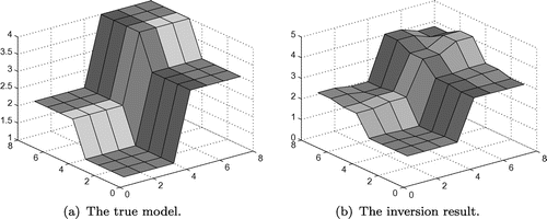
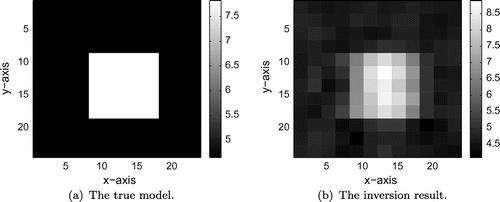
In this example we use AHPM. The non-linear diffusion function is $N(u)=u^4+u^3+u^2+u+1$, $h=1/10$, $Q^0\equiv 1$, and 5% Gaussian noise is added to the observed data. The true model and inversion result are shown in Figure 1.

Figure 1. The true model and inversion result with 5% Gaussian noise added in Example 4.2.

Example 4.3:

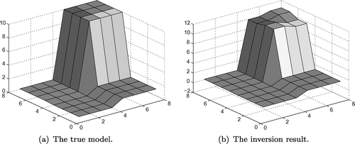
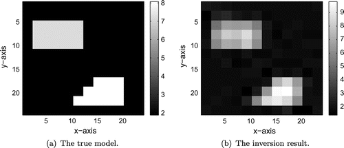
In oil reservoirs the permeability usually has greatly large jumps, so we use AHPM with $q_i^c={10}^{i-3}$, $i=1,\dots ,4$. The non-linear diffusion function is $N(u)=u^4-u^3+u^2-u+1$, $h=1/10$, $Q^0\equiv 1$, and 5% Gaussian noise is added to the observed data. The true model and inversion result are shown in Figure 2.

Figure 2. The true model and inversion result with 5% Gaussian noise added in Example 4.3.

It can be seen from these two examples that the adaptive homotopy perturbation method has good robustness, and is effective for the different N-functions, even if N is highly non-linear. Moreover, in Example 4.3, the basic iterative method is not convergent when the initial guess is chosen as an arbitrary constant. Hence, we conclude that the homotopy perturbation procedure is effective and even necessary in oil reservoir simulation.

Example 4.4:

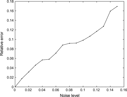
To further test the ability of dealing with noise of the proposed algorithm, we add 1%, 2%, $\dots$, 15% Gaussian noise to the observed data, respectively. In this example, we also use AHPM, and let $Q^0\equiv 1$, $h=1/10$. Figure 3 plots the relative $l^2$ errors vs. different Gaussian noise levels.

Figure 3. The relative $l^2$ errors with respect to different Gaussian noise levels in Example 4.4.

From this example, we can see that the relative $l^2$ errors are satisfactory under noisy background conditions. And from Figure 3, we can easily conclude that the adaptive homotopy perturbation method has good robustness.

Example 4.5:

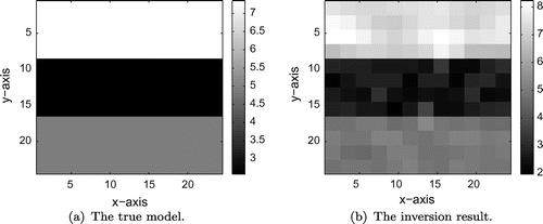
In this example, we consider a level-stratified medium containing two interfaces, which is depicted in Figure 4(a). Choose $h=1/10$, $Q^0\equiv 10$, and 1% Gaussian noise is added to the observed data. Figure 4(b) shows the inversion result, which is obtained by 9 iterations of AHPM. Starting from the same initial guess, BIM is not convergent, and HPM needs about 13 steps of iterations.

Figure 4. The true model and inversion result with 1% Gaussian noise added in Example 4.5.

Example 4.6:

In this example we consider the model of one anomalous body in a homogeneous medium with a permeability of 4.65, and the anomalous body has the permeability of 7.82. Choose $h=1/10$, $Q^0\equiv 10$, and 1% Gaussian noise is added to the observed data. Figure 5 shows this model and the inversion result obtained by 9 iterations of AHPM. Starting from the same initial guess, BIM is not convergent, and HPM needs about 12 steps of iterations.

Figure 5. The true model and inversion result with 1% Gaussian noise added in Example 4.6.

Example 4.7:

In this example we consider the model of two anomalous bodies in a homogeneous medium with a permeability of 1.88. The anomalous bodies have the permeability of 7.12 and 8.07, respectively. Choose $h=1/10$, $Q^0\equiv 10$, and 1% Gaussian noise is added to the observed data. Figure 6 shows this model and the inversion result obtained by 10 iterations of AHPM. Starting from the same initial guess, HPM needs about 13 steps of iterations. For this model, BIM is not convergent when the initial guess is chosen as an arbitrary constant.

Figure 6. The true model and inversion result with 1% Gaussian noise added in Example 4.7.

The numerical results in Examples 4.5–4.7 show that when the models are large-scale and complicated, (1) AHPM and HPM provide larger convergence regions than BIM; (2) AHPM is more computationally efficient against HPM; (3) AHPM has good robustness. So we can easily conclude that the merits of the adaptive homotopy perturbation method, such as the global convergence, computational efficiency and good robustness, still exist for the large-scale and complicated models (Figure 6).

5. Conclusions

This paper successfully designs an adaptive homotopy perturbation method for the identification of diffusion parameters in a non-linear convection–diffusion equation. Numerical simulations show that this new method has global convergence, computational efficiency and good robustness. Furthermore, the homotopy perturbation technique is not only effective for the different highly non-linear N-functions, but also necessary in oil reservoir simulation due to the greatly large jumps in the permeability.

Acknowledgements

The authors are grateful to anonymous referees for their valuable comments. The authors would like to thank Professor George Dulikravich and the typesetting team for their kind help.

Additional information

Funding

This work was supported by the National Natural Science Foundation of China [grant number 11271102]; the Natural Science Foundation of He-bei Province of China [grant number A2017501001]; the Science and Technology Funds for the Universities in He-bei Province of China [grant number Z2015039]; the Fundamental Research Funds for the Central Universities [grant number N142303011]; the PhD Foundation of Northeast University at Qinhuangdao [grant number XNB2015002].

Notes

No potential conflict of interest was reported by the authors.

Appendix 1

The numerical flux function

This appendix gives an explicit formula for the Engquist–Osher numerical flux functions $f^{EO}$ and $g^{EO}$. For simplicity, only one subscript index is used in the following calculations.

Buckley–Leverett flux function with gravitational effects

The flux function in the x-direction is an S-shaped Buckley–Leverett flux function with gravitational effects, see Equation (4.1(4.1) $$\begin{array}{c}\hfill f(u)=\frac{u^2(1-5(1-u^2))}{u^2+{(1-u)}^2},\end{array}$$(4.1) ). To calculate ${\int }_{u_i}^{u_{i+1}}|f^{\prime }(\mathit{\xi })|\mathrm{d}\mathit{\xi }$, the sign of $f^{\prime }$ in (0, 1) is studied first. $f^{\prime }$ has only one zero point in (0, 1), and this zero point is given by$$x_{zero}\approx 0.37.$$

So, it is easy to find that$$f^{\prime }(\mathit{\xi })\left\{\begin{array}{cc}<0,\hfill & \mathit{\xi }\in (0,x_{zero}),\hfill \\ =0,\hfill & \mathit{\xi }=x_{zero},\hfill \\ >0,\hfill & \mathit{\xi }\in (x_{zero,1}).\hfill \end{array}\right.$$

Then$${\int }_{u_i}^{u_{i+1}}|f^{\prime }(\mathit{\xi })|\mathrm{d}\mathit{\xi }=\left\{\begin{array}{cc}f(u_{i+1})-f(u_i),\hfill & u_i,u_{i+1}\ge x_{zero},\hfill \\ f(u_i)-f(u_{i+1}),\hfill & u_i,u_{i+1}<x_{zero},\hfill \\ f(u_i)+f(u_{i+1})-2f(x_{zero}),\hfill & u_i<x_{zero},u_{i+1}\ge x_{zero},\hfill \\ 2f(x_{zero})-f(u_i)-f(u_{i+1}),\hfill & u_i\ge x_{zero},u_{i+1}<x_{zero}.\hfill \end{array}\right.$$

By the definition of $f^{EO}$, we can get$$f^{EO}(u_i,u_{i+1})=\left\{\begin{array}{cc}f(u_i),\hfill & u_i,u_{i+1}\ge x_{zero},\hfill \\ f(u_{i+1}),\hfill & u_i,u_{i+1}<x_{zero},\hfill \\ f(x_{zero}),\hfill & u_i<x_{zero},u_{i+1}\ge x_{zero},\hfill \\ f(u_i)+f(u_{i+1})-f(x_{zero}),\hfill & u_i\ge x_{zero},u_{i+1}<x_{zero}.\hfill \end{array}\right.$$

Buckley–Leverett flux function

The flux function in the y-direction is an S-shaped Buckley–Leverett flux function, see Equation (4.2(4.2) $$\begin{array}{c}\hfill g(u)=\frac{u^2}{u^2+{(1-u)}^2}.\end{array}$$(4.2) ). Notice that$$g^{\prime }(u)\ge 0,u\in (0,1).$$

It is easy to find$$g^{EO}(u_i,u_{i+1})=g(u_i).$$

References

- Espedal MS, Karlsen KH. Numerical solution of reservoir flow models based on large time step operator splitting algorithm. In: Fasano A, editor. Filtration in porous media and industrial applications: lecture notes in mathematics. Vol. 1734. Berlin: Springer; 2000. p. 9–77.
- Luce R, Perez S. Parameter identification for an elliptic partial differential equation with distributed noisy data. Inverse Probl. 1999;15:291–307.
- Feng T, Yan N, Liu W. Adaptive finite element methods for the identification of distributed parameters in elliptic equation. Adv Comput Math. 2008;29:27–53.
- Chan TF, Tai XC. Identification of discontinuous coefficients in elliptic problems using total variation regularization. SIAM J Sci Comput. 2003;25:881–904.
- Chen Z, Zou J. An augmented Lagrangian method for identifying discontinuous parameters in elliptic systems. SIAM J Control Optim. 1999;37:892–910.
- Ito K, Kunisch K. The augmented Lagrangian method for parameter estimation in elliptic systems. SIAM J Control Optim. 1990;28:113–136.
- Li L, Liu W, Han B. Dynamical level set method for parameter identification of nonlinear parabolic distributed parameter systems. Commun Nonlinear Sci Numer Simulat. 2012;17:2752–2765.
- Tai XC, Kärkkäinen T. Identification of a nonlinear parameter in a parabolic equation from a linear equation. Comp Appl Mat. 1995;14:157–184.
- Hasanov A, DuChateau P, Pektaş B. An adjoint problem approach and coarse-fine mesh method for identification of the diffusion coefficient in a linear parabolic equation. J Inverse Ill-Posed Probl. 2006;14:435–463.
- Yang L, Yu JN, Deng ZC. An inverse problem of identifying the coefficient of parabolic equation. Appl Math Model. 2008;32:1984–1995.
- Cuypers M, Dubrule O, Lamy P, et al. Optimal choice of inversion parameters for history matching with the pilot point method. In: Proceedings of the 6th European Conference on the Mathematics of Oil Recovery; Peebles, UK; 1998.
- Grimstad AA, Mannseth T, Nordtvedt JE, et al. Reservoir characterization through scale splitting. In: Proceedings of the 7th European Conference on the Mathematics of Oil Recovery; Baveno, Italy; 2000.
- Reynolds AC, He N, Chu L, et al. Reparameterization techniques for generating reservoir descriptions conditioned to variograms and well-test pressure data, SPE 30588. In: Proceedings of the SPE Annual Technical Conference and Exhibition; Dallas, USA; 1995.
- Shah PC, Gavalas GR, Seinfeld JH. Error analysis in history matching, the optimum level of parameterization. Soc Pet Eng J. 1978;6:219–228.
- He JH. Homotopy perturbation technique. Comput Method Appl M. 1999;178:257–262.
- He JH. A coupling method of a homotopy technique and a perturbation technique for non-linear problems. Int J Nonlinear Mech. 2000;35:37–43.
- He JH. Homotopy perturbation method: a new nonlinear analytical technique. Appl Math Comput. 2003;135:73–79.
- He JH. The homotopy perturbation method for nonlinear oscillators with discontinuities. Appl Math Comput. 2004;151:287–292.
- He JH. Application of homotopy perturbation method to nonlinear wave equations. Chaos Soliton Fract. 2005;26:695–700.
- He JH. Comparison of homotopy perturbation method and homotopy analysis method. Appl Math Comput. 2004;156:527–539.
- Li X, Xu M, Jiang X. Homotopy perturbation method to time-fractional diffusion equation with a moving boundary condition. Appl Math Comput. 2009;208:434–439.
- Mohyud-Din ST, Yildirim A. Homotopy perturbation method for advection problems. Nonlinear Sci Lett A. 2010;1:307–312.
- Nilssen TK, Karlsen KH, Mannseth T, et al. Identification of diffusion parameters in a nonlinear convection-diffusion equation using the augmented Lagrangian method. Comput Geosci. 2009;13:317–329.
- Rajeev S. Homotopy perturbation method for a Stefan problem with variable latent heat. Therm Sci. 2014;18:391–398.
- Zhou G, Wu B. Application of the homotopy perturbation method to an inverse heat problem. Int J Numer Method H. 2014;24:1331–1337.
- Hetmaniok E, Nowak I, Słota D, et al. Solution of the inverse heat conduction problem with Neumann boundary condition by using the homotopy perturbation method. Therm Sci. 2013;17:643–650.
- Hetmaniok E, Nowak I, Słota D, et al. Application of the homotopy perturbation method for the solution of inverse heat conduction problem. Int Commun Heat Mass. 2012;39:30–35.
- Słota D. The application of the homotopy perturbation method to one-phase inverse Stefan problem. Int Commun Heat Mass. 2010;37:587–592.
- Słota D. Homotopy perturbation method for solving the two-phase inverse Stefan problem. Numer Heat Tr A-Appl. 2011;59:755–768.
- Shakeri F, Dehghan M. Inverse problem of diffusion equation by He’s homotopy perturbation method. Phys Scripta. 2007;75:551–556.
- Engquist B, Osher S. One-sided difference approximations for nonlinear conservation laws. Math Comput. 1984;36:321–351.