Inverse identification of impact locations using multilayer perceptron with effective time-domain feature

Abstract

This study presents a novel time-domain feature to identify impact locations using Multilayer Perceptron. This feature is based on the minimum arrival time (MAT) of surface wave at a particular location of an object due to impact. Trial impact forces were made on a Perspex plate structure and corresponding acceleration responses were acquired from six locations. Two other conventional time-domain features – peak arrival time (PAT) and threshold crossing (TC), were compared with the proposed feature. Each feature was used separately as network inputs to identify 15 fixed impact locations. The results showed that impact localization with MAT feature resulted in the highest accuracy, making a relative decrease in error of 42.06 and 81.04% compared to PAT and TC cases, respectively. A consistency measurement scheme has been developed as well, which indicated that MAT is more consistent than PAT and TC for a particular pair of impact-sensor location, and hence a more accurate localization of impact can be obtained.

Keywords:

• Feature consistency
• feature extraction
• impact force
• impact localization
• multilayer perceptron

AMS Subject Classifications:

• 62P30
• 74M20
• 68T05
• 92B20

1. Introduction

Impact force is more likely to cause damage to any structure than any other external forces because it acts for a very short duration with relatively high magnitude which excites several natural frequencies within the structure. In other words, the impacted body does not get enough time to deform and vibrate; so it behaves more brittle than usual. Thus, identification of impact force is crucial to spot the actual damage location and severity to help the proper maintenance of any structure. Direct identification of impact forces by simply mounting force transducers is not feasible in most of the cases due to various ambient conditions such as random thrust forces from large compressor to its base, impact forces to a building column, bump forces to a moving vehicle due to rough roads, motor torque pulses and forces from fluid pressure in pipelines. Even if the structure is placed in a viable position, it will require a large number of sensors. Therefore, indirect/inverse methods to reconstruct impact forces have attracted much interest among the researchers [1–4].

In general, indirect identification techniques can be categorized into two kinds: time-domain and frequency-domain techniques. Frequency domain approaches include Fourier transformation of responses over a certain period of sample signals at partial or complete stable condition and multiplying its inverse form by a transfer function. However, the inversion action turns the transfer functions ill-conditioned near the region of the resonance frequency. For this reason, various regularization methods are applied such as Singular Value Rejection method, Tikhonov method [5], Singular Value Decomposition (SVD) method [6] and Truncated SVD method [7,8] in order to obtain stable solutions for different ill-posed problems. However, frequency-domain methods are problematic in case of non-steady-state conditions, e.g. subjection of impact forces, because it takes a certain length of stationary time to compute the inverse Frequency Response Function (FRF) matrix for each frequency reading. Another notable disadvantage is that if a FRF matrix which has a high condition number is inversed, slight measurement errors or noises will be amplified significantly and will result in larger errors in the reconstruction of the forces.

On the other hand, time-domain methods have become much popular in the field of force identification because it provides real-time information about the impact or varying force and can deal with both stationary and non-stationary forces. Based on past studies, most of the previous time-domain approaches can be categorized into three sub-methods which are wave arrival time estimation [9–14], optimization [15–17] and artificial neural network (ANN) methods [18–25]. Often these methods are applied in combination to achieve better accuracy [10,26]. A notable drawback of wave arrival time methods is their dependency on correct evaluation of wave arrival time which is intricate since wave propagation can be disrupted considerably by any slight structural irregularity. Limitations of optimization methods are that they need a proper mathematical model/objective function to bridge the input–output relation and a close initialization of variables to the actual solution. Thereby, ANNs have drawn a significant attention in recent years, since they can avoid the mentioned drawbacks and provide higher accuracy. It is because ANNs are proficient at generalizing an input–output relationship based on a package of sample data-sets provided to it, without the need of any extra mathematical model. Whereas other methods get affected by non-linearity in forces or surrounding uncertainties/noises, ANNs show strong tolerance against such odds when trained accordingly. This is why ANNs are effective in many different practical applications [27–31].

Since time domain gives better information on the impact event than frequency domain, most of the ANN-based impact identification approaches used time-domain features as inputs. However, selection of proper input feature from vibration signal is challenging due to the complex elastic behaviour of test rigs. To the authors’ best of knowledge, previous ANN approaches on impact force localization were mostly based on the arrival time of surface wave in terms of threshold-crossing [20,24] or peak amplitude [26,32]. These features do not represent the exact arrival time of surface wave, but they are useful to train the ANNs to localize impacts. However, due to heterogeneity of material, e.g. density variation or presence of sporadic porosity, the propagated elastic waves change their waveform by experiencing superposition with their refraction and/or reflection within the object. Thereby, the temporal waveform obtained from surface-mounted sensor may change its shape which will cause deviation in the extracted feature values.

This paper proposes a different time-domain feature which provides better estimation of wave arrival as well as being more robust to noise than the conventional features. Multilayer Perceptron (MLP), which was used in each of the past similar studies, has been used here as well to compare the effectiveness of the proposed and popular features. Only impact localization has been studied here since the proposed feature was chosen for better identification of impact locations as it is distance variant but amplitude invariant.

2. Impact localization methodology

2.1. Feature extraction

Due to the large amount of acceleration data for each response of an accelerometer, the feature extraction procedure is required to obtain the neural network inputs. Most commonly used time-domain features in ANN-based impact localization are peak arrival time (PAT) [20,22,24–26,33]. PAT is basically based on the maximum energy arrival concept which roughly estimates the surface wave arrival time. However, since the test plate is not absolutely homogeneous, scattering of waves may occur in some places due to erratic reflection and refraction of elastic waves. This is called dispersion effect [34] which results in change of shape of time-domain signal due to the superposition of scattered waves [35]. Besides, such shape change is not uniform for a pair of impact-sensor location because of a variety of the given impacts (intensity and duration). Therefore, PAT occasionally gives an erroneous estimation of surface wave arrival and may change with different same-located impacts.

Another popular feature, Threshold-Crossing (TC), is also a time measurement which picks the first crossing time of signal’s amplitude over a predefined threshold value. It also gives a rough measurement of wave arrival time based on when a sensor starts vibrating with respect to a reference time.

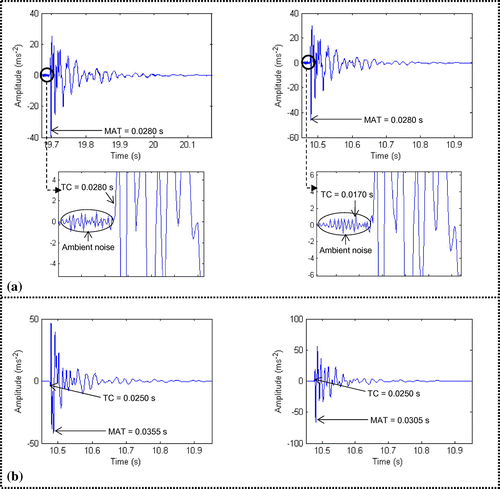
Several studies used TC [24,25,32] as a feature for impact localization. However, in real world, ambient boundary conditions may change time-to-time or place-to-place, which may introduce noise above the threshold value. This would cause a significant shift of TC value for same-located trial impacts as shown in Figure 2(a). Besides, this feature requires a very high sampling rate to achieve the optimum resolution of measurement because the threshold-crossing at a nearby sensor occurs due to combined multiple elastic waves propagating at hypersonic velocity. That is, if the sampling rate is low, TC values at two different locations (with a notable radial distance difference from the source) might be the same (Figure 2(b)), which would be problematic to build proper input vectors for ANNs to localize impacts.

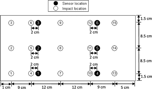
According to several impact-echo studies [36–38], when a sensor is attached to the same surface and nearby of a point-source of impact force, the waveform obtained from the sensor reading will possess a large downward amplitude (minima) which occurs due to the surface wave. This downward waveform will continue to propagate radially along the plate surface with certain attenuation rate. Thereby, considering all these, we hypothesize that instead of taking PAT, minima arrival time (MAT) would give a much better estimation of surface wave arrival and better consistency for different impacts. Figure 1 shows two experimental examples which support this hypothesis. See Sec. 3 about the impact and sensor locations mentioned in Figure 1. Furthermore, MAT avoids the mentioned difficulties of TC by being invariant to ambient noises (Figure 2(a)) and variant to impact-sensor distance (Figure 2(b)), which makes it a more effective feature for identifying impact locations.

Figure 1. Discrepancy of PAT than MAT for two same-located impacts when (a) impact location 1 and sensor 4 (b) impact location 14 and sensor 5.

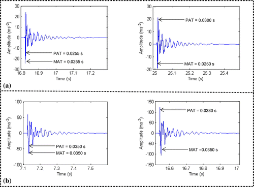
Figure 2. (a) Deviation of TC (at sensor 1) due to ambient noise for two separate impacts at location 3 (b) Non-variety of TC at sensors 10 and 12 for impact at location 3. (sensor’s radial distance difference from impact source = 4.5 cm)

Therefore, these three features have been used here separately as inputs to the network for comparison. Setting the threshold value at 1 ms⁻² amplitude by experimental observation as follows Refs. [24,32], extraction of PAT, MAT and TC can be expressed in Equations (1(1) $$F_{\text{PAT}}=min\left\{t\ge 0:\left|v\left(t\right)\right|=max\left(\left|v\left(t\right)\right|\right)\right\}-t_0$$(1) )–(3(3) $$F_{\text{TC}}=inf\left\{t\ge 0:\left|v\left(t\right)\right|>1\right\}-t_0$$(3) ), respectively.

(1) $$F_{\text{PAT}}=min\left\{t\ge 0:\left|v\left(t\right)\right|=max\left(\left|v\left(t\right)\right|\right)\right\}-t_0$$(1)

(2) $$F_{\text{MAT}}=min\left\{t\ge 0:v\left(t\right)=min(v\left(t\right))\right\}-t_0$$(2)

(3) $$F_{\text{TC}}=inf\left\{t\ge 0:\left|v\left(t\right)\right|>1\right\}-t_0$$(3)

where v(t) – time-domain acceleration signal; F – feature method; t₀ – initial time of time-domain response window.

2.3. Multilayer perceptron

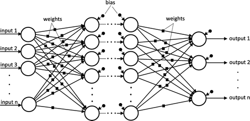
MLP has been the most frequently used supervised neural network model because of its simplicity to perform universal approximation. A MLP includes one input layer, one or multiple hidden layers and one output layer (Figure 3). Hidden layer architecture does not proportionally affect the accuracy of MLP. However, Hecht-Nielsen proved that ANN with one hidden layer is capable to perform universal approximation [39]. This is why MLP with one hidden layer was adopted in this study.

Figure 3. General topology of MLP.

MLP is mostly trained with backpropagation training algorithms such as Levenberg–Marquardt, Resilent Backpropagation and Conjugate Gradient. The name ‘Backpropagation’ came from the nature of the error optimization procedure in backward direction, i.e. from the output layer to the input layer. In this study, the NEWFF function in MATLAB® was used with Levenberg–Marquardt (LM) training function (‘trainlm’) at default settings (See Ref. [40]) to build the network, which is given by,

$$\text{net = newff}\left(P,T,S\right)$$

where P, T and S are input vector, output vector and hidden layer size, respectively.

The default activation functions for MLP’s hidden layer and output layer neurons are hyperbolic tangent sigmoid (Equation (5(5) $$y_h=\frac{e^u-e^{-u}}{e^u+e^{-u}}$$(5) )) and linear function (Equation (6(6) $$y_o=b_o+w_o{y}_h$$(6) )), respectively. The net function, whose value is the only independent variable of the activation functions, takes the inputs and processes them with weights and bias as Equation (4(4) $$u=b_h+\sum _{j=1}^N{w}_j{x}_j$$(4) ).

Thereby, from Equations (4(4) $$u=b_h+\sum _{j=1}^N{w}_j{x}_j$$(4) )–(6(6) $$y_o=b_o+w_o{y}_h$$(6) ), the only parameter that is adjusted are the connection weights (w) between neurons. To obtain desired w, LM [41] was selected as the training algorithm. This is because it provides more accurate and faster training than other backpropagation algorithms, especially when the application type is function approximation and network possesses few hidden neurons [42], like the case of this study.

(4) $$u=b_h+\sum _{j=1}^N{w}_j{x}_j$$(4)

(5) $$y_h=\frac{e^u-e^{-u}}{e^u+e^{-u}}$$(5)

(6) $$y_o=b_o+w_o{y}_h$$(6)

where u – weighted inputs to a hidden neuron; x – inputs (=y_h for output neurons); N – number of inputs; w_j – weight values for inputs (w_j: 1 ≤ j ≤ N); w_o – weight value for the hidden neuron’s output; b_h – hidden neuron’s bias weight; b_o – output neuron’s bias weight; y_h and y_o – output from hidden and output layer neuron, respectively.

3. Experimental setup and procedure

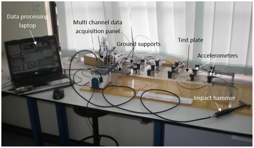
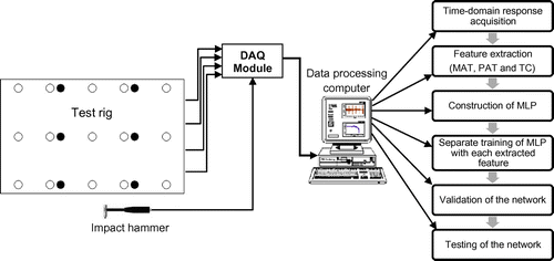
All the data used in this study are from a previous study [43] where a rectangular Perspex plate, having a dimension of 48cm × 20cm × 0.9cm, was used as the test specimen as shown in Figure 4. It was ground supported at its four corners with combined aluminium and steel plates. By considering the practical usage of lower amount of sensors, we only used 6 out of the 15 sensors’ recording obtained from the earlier experiment. Without knowing the optimum selection of sensor combination, these six sensors were selected in symmetric arrangement from the centre of the test rig, and it is fixed throughout the experiments to ensure consistency in the collected data. These sensors are model S100C Wilcoxon Research Integrated Circuit Piezoelectric accelerometers, which were mounted in a certain order on the plate (Figure 5) with cyanoacrylate adhesive. All response data from the accelerometers were collected via multiple channel data acquisition hardware comprising of four-channel DAQ module and a DAQ chassis. This system was connected to a computer to post-process the collected data via DASYLab® and MATLAB®. A modally tuned impact hammer was taken to generate the impact excitations as well as to record the force data. Since repeated impacts were made onto the specified locations, the precision of impacts was approximately 2 radial cm around a location’s centre. Corresponding responses from the accelerometers for each individual impact were recorded via DASYLab® obtained through the DAQ module. The sampling rate and block size were 2000 Hz and 4096 samples, respectively. Each block consisted of a pre-trigger value of 50 samples, that is in each time response data, first 50 samples were the pre-impact response and the rest 4046 samples were the post-impact response. For auto data collection, a threshold limit of 3N was set so that impacts over this limit would start recording the responses as time-domain data. A total of 55 sets of response data, each of which consists of single impacts at all specified locations, were recorded. Training and testing impacts were given at 15 locations as shown in Figure 5.

Figure 4. Experimental set-up for impact identification study.

Figure 5. Arrangement of the sensors and impact locations.

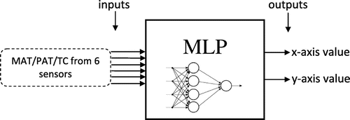
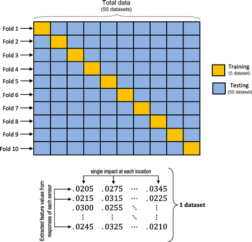
After acquiring all the responses, MATLAB® was used to run the feature extraction process from the raw signals as described in Section 2.1 and also to train the MLP in order to predict the impacts. The feature extraction procedure was repeated for every single response data of each sensor. The network inputs were MAT/PAT/TC features from six sensors and the outputs were the Cartesian coordinates, i.e. x and y axis values of the locations (Figure 6). The network prediction error was evaluated by Euclidean distances between corresponding predicted and measured locations. To validate the architecture of the network, 10-fold cross validation was followed with different hidden layer sizes for each feature. This cross validation procedure is based on running the network with 10 randomly selected subsamples containing training and testing data (Figure 7) in order to reduce the influence of training and testing data selection. It will also reveal the accuracy of the features over different folds/subsamples. Since each data-set consists of similar impact-response events, the cross validation was designed to train the network with fewer data-sets and testing with larger data-sets. This would reveal the consistency of accuracy of the features over different test impacts. Thereby, at each fold, five randomly chosen data-sets were used for training and the rest 50 sets of data were used for testing. Error goal was set to 0.1 MSE (mean-square error) as absolute zero is likely to cause overfitting. Figure 8 visually demonstrates the overall experimental procedure of impact localization in this study.

Figure 6. Impact localization and impact quantification scheme.

Figure 7. Structure and distribution of data in different stages.

Figure 8. Schematic diagram of the experimental procedure.

4. Results and discussion of experimental impact localization

Impact localization results using MAT, PAT and TC have been discussed in this section. Table 1 shows the accuracy of the network (in terms of mean radial cm error) for different hidden layer sizes at different folds/subsamples using all selected features separately. It can be seen that MLP’s approximation ability does not actually rely on increasing No. of hidden neurons. There is an optimum point after which network’s error is likely to increase due to overfitting. Therefore, based on Table 1, three separate networks with 15, 11 and 6 hidden neurons were found to be the optimum network architecture for MAT, PAT and TC, respectively. Table 1 also shows that MAT gives the best average accuracy for any hidden layer size and subsample, where with the optimum network size, MAT’s mean error ranges from 0.53 to 1.02 mean radial cm over different folds/subsamples.

Table 1. The effect of hidden neurons with different features and subsamples.

MAT
No. of hidden neurons	Mean error (radial cm) of the subsequent subsample										Average
	1	2	3	4	5	6	7	8	9	10
3	1.09	1.07	1.07	0.97	1.14	1.17	1.20	0.97	1.62	1.10	1.14
5	0.80	1.02	0.86	0.73	0.75	0.98	1.30	0.85	0.95	0.66	0.89
6	0.91	0.92	1.00	0.68	0.97	0.97	0.88	0.70	0.85	0.81	0.87
10	0.91	0.81	0.94	0.63	0.92	1.24	0.78	0.75	0.77	0.67	0.84
11	0.83	0.76	0.91	0.77	0.96	1.13	0.75	0.87	0.89	0.80	0.87
13	1.05	0.77	1.13	0.83	1.64	1.23	1.05	0.75	0.67	0.97	1.01
15	0.60	0.77	0.92	0.73	1.02	0.70	0.74	0.67	0.53	0.88	0.76
17	0.92	0.82	0.73	1.01	1.22	1.38	1.14	0.87	0.77	0.85	0.97
19	0.81	0.90	0.91	1.23	1.10	1.20	0.94	0.77	0.73	1.09	0.97
20	0.88	0.87	0.89	0.66	1.27	1.27	0.94	0.85	0.77	0.93	0.93
23	0.83	1.22	1.07	0.77	1.48	1.25	0.84	0.89	0.74	0.99	1.01
25	1.00	0.74	1.16	0.72	1.23	0.92	0.82	1.03	0.75	1.36	0.97
PAT
3	3.24	3.60	2.98	3.53	4.12	2.74	4.22	6.07	3.66	2.87	3.70
5	2.25	2.07	1.80	2.54	2.78	12.70	2.11	2.06	2.28	1.75	3.23
6	1.53	1.70	2.28	2.22	2.25	2.51	1.60	2.26	2.24	2.33	2.09
10	1.22	2.04	2.20	1.78	2.14	2.89	1.65	1.76	1.60	2.89	2.02
11	1.17	1.43	1.59	1.25	2.66	2.18	1.20	1.45	1.42	2.01	1.64
13	1.27	1.80	1.61	1.65	1.87	2.43	1.34	1.72	1.57	1.77	1.70
15	1.34	1.51	1.41	1.52	2.40	2.20	1.45	2.19	1.65	2.15	1.78
17	1.32	1.96	1.76	1.77	1.90	2.51	1.58	2.51	1.95	1.69	1.89
19	1.50	2.04	1.78	1.76	2.23	2.77	1.65	1.79	1.75	2.12	1.94
20	1.18	1.92	2.03	1.55	2.48	2.88	1.80	1.91	2.19	1.45	1.94
23	1.40	2.82	2.78	2.00	2.74	2.82	1.66	1.47	2.06	1.72	2.15
25	1.52	2.41	1.90	1.57	2.06	2.34	1.58	1.92	1.73	1.57	1.86
TC
3	3.25	3.56	3.43	3.89	3.62	6.08	16.32	3.49	3.46	3.48	5.06
5	3.28	3.63	3.42	6.47	7.31	5.26	13.36	5.35	3.35	3.70	5.51
6	6.10	3.58	4.38	3.86	4.25	4.09	4.03	8.98	6.41	4.60	5.03
10	4.65	9.42	4.78	7.37	3.89	16.25	8.02	8.30	10.06	7.42	8.02
11	4.58	5.44	5.53	12.43	9.24	13.48	10.33	6.15	8.05	4.31	7.95
13	5.49	4.73	6.82	5.02	6.34	8.23	6.49	4.31	5.79	4.78	5.80
15	6.02	7.36	5.87	5.45	5.64	10.95	8.80	6.94	5.24	8.41	7.07
17	8.46	5.40	6.41	8.17	5.10	9.07	3.99	6.13	8.83	6.64	6.82
19	5.53	6.53	9.58	4.89	6.48	9.36	6.39	5.47	5.58	7.81	6.76
20	10.72	4.88	7.62	6.24	8.46	6.26	7.36	10.57	7.52	8.48	7.81
23	6.70	6.94	4.92	6.42	5.48	4.77	10.25	6.53	5.71	8.07	6.58
25	6.39	6.69	5.90	6.69	7.09	8.19	6.81	8.36	7.72	5.61	6.94

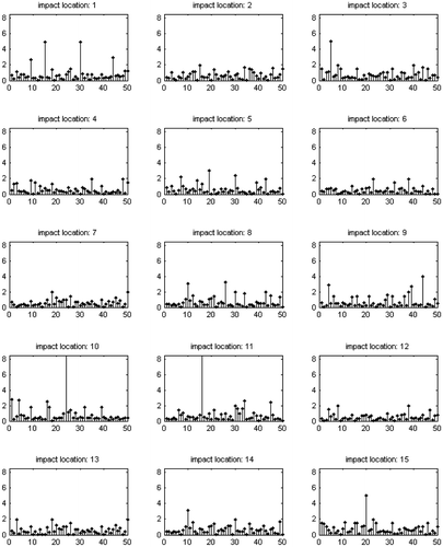
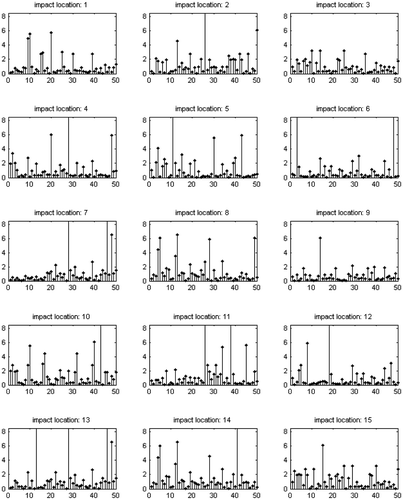
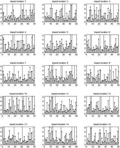
Now, picking the detailed results from a random subsample (subsample 4) when using the optimum network architectures, Figures 9–11 represent the impact localization performances of MAT, PAT and TC, respectively, over different test impacts. The minimum distance between two impact locations is 8.5 cm; so MLP’s prediction error is limited to 8.5 radial cm in each subfigure of Figures 9–11. Figure 9 shows that all 15 impact locations were identified with a very low radial cm error using MAT. Considering all impact locations and test impacts, the mean error estimated in this case was 0.73 radial cm. Figure 10 shows that the error is higher for most of the locations and most of the trial impacts when PAT is used. In this case, the mean error found to be 1.26 radial cm. From Figure 11, it is obvious that error level is consistently much higher for almost every impact location than that of MAT and PAT, which is why the mean error found in this case was 3.85 radial cm. Table 2 represents the mean approximation error at each location using the selected features and it shows that MAT is better in identifying any location than PAT and TC. In overall, impact localization with MAT feature resulted in the highest accuracy, making a relative decrease in error of 42.06% and 81.04% compared to PAT and TC cases, respectively.

Figure 9. Impact localization error (radial cm) vs. no. of test impacts using MAT.

Figure 10. Impact localization error (radial cm) vs. no. of test impacts using PAT.

Figure 11. Impact localization error (radial cm) vs. no. of test impacts using TC.

Table 2. Mean approximation error at individual locations.

Features	Mean classification error (radial cm) at subsequent location															Average
	1	2	3	4	5	6	7	8	9	10	11	12	13	14	15
MAT	0.82	0.67	0.78	0.58	0.63	0.50	0.57	0.70	0.70	1.38	1.12	0.52	0.60	0.68	0.80	0.73
PAT	1.00	1.35	0.95	1.26	1.41	1.19	1.25	1.32	0.73	1.52	1.53	1.06	1.58	1.47	1.26	1.26
TC	3.70	4.12	5.07	2.91	2.83	5.02	2.83	3.92	3.85	4.28	3.36	4.84	3.52	3.99	3.43	3.85

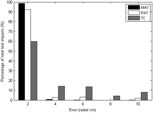
A histogram (Figure 12) was built with the results from Figures 9–11 which shows the error spread of total test impacts. Refering to this histogram, 98.67% of test impacts were localized within the error range of 2 radial cm using MAT, whereas PAT and TC were able to localize 92.27 and 58.13% test impacts, respectively, within this range. Besides, unlike MAT, a significant percentage of test impacts were predicted with high abrupt errors (4 radial cm and above) using PAT and TC. Apart from the current subsample, similar accuracy can be found using the other nine subsamples as well, where the average success rate of MAT, PAT and TC estimated within 2 radial cm error was 96.72, 87.58 and 58.79%, respectively (Table 3). Besides that, the bounds of MAT’s, PAT’s and TC’s success rates were 94.13–99.20, 77.20–93.67 and 52.93–66.13%, respectively, throughout all 10 subsamples. Thereby, in overall, the impact localization with MAT has the highest success rate, followed by PAT and TC. However, there are several trial impacts resulted in high error in all cases. The results show that the success rate of impact localization can be improved using a suitable feature, where MAT results in the least localization error, followed by PAT and TC.

Figure 12. Performance histogram of the selected features for impact localization (subsample 4).

Table 3. Success rate percentage of the features for different subsamples.

Features	Success rate (%) within 2 radial cm error for subsequent subsample										Average
	1	2	3	4	5	6	7	8	9	10
MAT	97.20	96.40	97.07	98.67	94.93	95.33	99.20	97.33	96.93	94.13	96.72
PAT	93.67	91.60	89.87	92.27	77.20	79.87	90.80	89.33	90.53	80.67	87.58
TC	58.40	66.13	56.80	58.13	65.33	54.67	58.27	52.93	55.47	61.73	58.79

The localization error may be due to the possible presence of measurement noises and uncertainties, such as the effectiveness of MLP for impact localization application and the usage of non-optimum combination of sensor location. Another limitation of this study is the collocation of training and testing impacts (i.e. they are being at the same place). It was designed in such a way that it could avoid any other uncertainties that may appear due to location difference between training and testing impacts. This is useful for some problems (e.g. identification of impact force acting on a vehicle passing through road bump; identification of ship collision/ wave impact acting on offshore structure), where the impact location of interest is known in a priori, and the training and testing impacts are collocated in the same position. However, for many other real-life applications, the goal is to identify impacts at any arbitrary locations where the impact location is unknown in a priori. These effects have not been considered in the scope of this study. So, it is expected that the accuracy of the impact localization can be further enhanced using a more advanced algorithm (e.g. Sigma-if [44,45], Generalised Regression Neural Network [46,47], etc.), optimum sensor combination as well as scattered impact locations in future work.

In Table 4, impact localization errors (radial cm) of few similar previous studies have been provided. Comparing the PAT result provided in Tables 2 and 4, Refs. [26] and [33] gave 3.46 and 1.64 mean errors (radial cm) with 4 and 17 sensors, respectively, while this study produces 1.26 mean error (radial cm) with 6 sensors. The range of errors obtained from these studies is within 1.26–1.64 radial cm for the usage of PAT feature. On the other hand, it can be seen that Refs. [24] and [25] produced higher accuracy using TC feature (i.e. 1.73 and 1.10 root mean-square errors), as compared to this study (i.e. 3.85 mean error). This is because the previous studies used a higher sampling frequency (200 kHz) and a large number of sensors (18 and 300, respectively), which may greatly improve the result. The range of errors obtained from these studies is within 1.10–3.85 radial cm for the usage of TC feature. Moreover, the proposed MAT feature produces the highest accuracy (i.e. 0.73 mean error (radial cm)) compared to all the examined results for PAT and TC features. Note that all the examined studies (Refs. [24–26,33] and this study) followed different designs of experiments such as different sampling rates, materials, number of sensors and neural network architecture, which affected the impact localization accuracy to different extents. Users should wisely select those parameters in order to achieve their desired accuracy, with reasonable computational time and affordable instrumentation and equipment costs. In this study, the impact localization accuracy varies only for different feature extraction methods, since other parameters/ factors (e.g. training and testing impact locations, No. of sensors, sampling rate, etc.) were fixed throughout the study. It shows that MAT is the best feature for impact localization problem compared to PAT and TC features.

Table 4. Impact localization accuracy of few similar earlier studies.

Refs.	Usage of feature	Error (radial cm)
Worden and Staszewski [26]	PAT	3.46 (mean)
Maseras-Gutierrez et al. [33]	PAT	1.64 (mean)
Sharif-Khodaei et al. [24]	TC	1.73 (RMSE)
Ghajari et al. [25]	TC	1.10 (RMSE)

Note: RMSE – root mean-square error.

Regarding this, the results here clearly support the effectiveness of MAT over PAT and TC. One major reason behind this is that the approximation performance of MLP gets weaker if the consistency/similarity between same-condition (i.e. impact at the same location) measurements becomes less. Regarding this factor, MAT is more consistent than PAT and TC for a particular pair of impact-sensor location. To quantify such consistency, mean standard deviation (MSD) has been adopted here as shown in Equations (7(7) $${\mathbf{R}}_k=\begin{array}{cccc}{F}_{1,1,k}^{\prime }\hfill & F_{1,2,k}^{\prime }\hfill & \cdots \hfill & F_{1,f,k}^{\prime }\hfill \\ F_{2,1,k}^{\prime }\hfill & F_{2,2,k}^{\prime }\hfill & \cdots \hfill & F_{2,f,k}^{\prime }\hfill \\ F_{3,1,k}^{\prime }\hfill & F_{3,2,k}^{\prime }\hfill & \ddots \hfill & F_{3,f,k}^{\prime }\hfill \\ ⋮\hfill & ⋮\hfill & \ddots \hfill & ⋮\hfill \\ F_{r,1,k}^{\prime }\hfill & F_{r,2,k}^{\prime }\hfill & \cdots \hfill & F_{r,f,k}^{\prime }\hfill \end{array}$$(7) )–(11(11) $$\text{MSD of}{F}^{\prime }=\frac{1}{mn}\sum _{r=1}^m\sum _{f=1}^n{s}_{r,f}$$(11) ). This quantification procedure is based on estimating the MSD of F’ values for a repeated impact-sensor location pair. Each input vector/cluster, which indicates responses from all sensors per impact, was normalised first and then MSD was applied on the same-condition input classes appeared through the repeated test impacts. After finding the MSD values for all impact-sensor pairs, the overall average of them was calculated to quantify a feature’s consistency.

(7) $${\mathbf{R}}_k=\begin{array}{cccc}{F}_{1,1,k}^{\prime }\hfill & F_{1,2,k}^{\prime }\hfill & \cdots \hfill & F_{1,f,k}^{\prime }\hfill \\ F_{2,1,k}^{\prime }\hfill & F_{2,2,k}^{\prime }\hfill & \cdots \hfill & F_{2,f,k}^{\prime }\hfill \\ F_{3,1,k}^{\prime }\hfill & F_{3,2,k}^{\prime }\hfill & \ddots \hfill & F_{3,f,k}^{\prime }\hfill \\ ⋮\hfill & ⋮\hfill & \ddots \hfill & ⋮\hfill \\ F_{r,1,k}^{\prime }\hfill & F_{r,2,k}^{\prime }\hfill & \cdots \hfill & F_{r,f,k}^{\prime }\hfill \end{array}$$(7) (8) $$F_{r,f,k}^{\prime }=\left\{\begin{array}{c}\frac{F_{r,f,k}-\text{min}(P)}{\text{max}(P)-\text{min}(P)},\text{max}(P)\ne \text{min}(P)\hfill \\ \hfill \\ 0,\text{otherwise}\hfill \end{array}\right.,\text{where}P=F_{r,f,k}:1\le r\le m$$(8)

(9) $$\overline{F_{r,f}^{\prime }}=\frac{1}{l}\sum _{k=1}^l{F}_{r,f,k}^{\prime }$$(9)

(10) $$s_{r,f}=\sqrt{\frac{1}{l-1}\sum _{k=1}^l{\left|F_{r,f,k}^{\prime }-\overline{F_{r,f}^{\prime }}\right|}^2}$$(10)

(11) $$\text{MSD of}{F}^{\prime }=\frac{1}{mn}\sum _{r=1}^m\sum _{f=1}^n{s}_{r,f}$$(11)

where F – selected feature; F′ – normalized feature; R_k – response’s feature matrix with each column normalized; l – total trials (k = 1, 2, ..., 55); m – total sensors (r = 1, 2, 3, …, 6); n – total impact locations (f = 1, 2, 3, …, 15); and s – standard deviation.

Table 5 shows the MSD of MAT, PAT and TC. From Table 4, it is obvious that MAT is the most consistent throughout all test impacts as its MSD value is the least (i.e. 0.0448). On the other hand, TC is the least consistent as it possesses the highest MSD value (i.e. 0.1063). Table 5 also shows the maximum standard deviation of the features where MAT < PAT < TC, which signifies the statistical similarity of the consistency measurement. This is why MAT gave the highest and TC gave the lowest accuracy to predict impact locations with MLP. It is worthwhile to mention that the selection of optimal sensor combination has not been performed in this study since the primary objective of this study is to compare the effectiveness of the features. Although the sensor placement in this study is symmetrical in relation to the test plate and impact locations, it is likely that asymmetrical sensor placement might influence the result since it would affect the pattern of input vectors. For example, Ref. [26] optimized the sensor placement using genetic algorithm, which was found to be asymmetrical in relation to the test plate and impact positions. This is why we are considering this issue as a potential future scope of the current study.

Table 5. Mean and maximum standard deviation for various features (when normalized).

Features	Mean standard deviation (MSD)	Maximum standard deviation
MAT	0.0448	0.2513
PAT	0.0861	0.4361
TC	0.1063	0.4389

5. Conclusion

In this study, a new time-domain feature, MAT was proposed as an effective input feature to identify impact locations using ANNs. Performance of MAT was compared with performances of two features: PAT and TC, which have been used in many different past studies on ANN-based impact localization. MLP was adopted here as the ANN algorithm because of its high-frequency uses in past similar experiments. Prediction results from cross validation show that MAT provides the highest accuracy (in terms of mean error) for any subsample and hidden layer size. Based on the validation result, optimum network was identified in each feature’s case. With optimum networks and a randomly chosen subsample, MAT was found to cause 42.06 and 81.04% relative decrease in error to localize impacts compared to PAT and TC, respectively. In the case of this subsample, MLP was able to localize 98.67% impacts below 2 radial cm error using MAT whereas PAT and TC gave lower success rates (i.e. 92.27 and 58.13% impacts below 2 radial cm error, respectively). By taking all 10 subsamples into account, the MAT’s average success rate was found to be 96.72%, whereas PAT’s and TC’s were 87.58 and 58.79%, respectively. These results clearly prove the robustness of MAT on MLP’s prediction performance. The reason identified behind such high accuracy is that MAT is more consistent than PAT and TC for a particular pair of impact-sensor location. This is supported by the consistency measurement of MAT, PAT and TC features (i.e. MSD value of 0.0448, 0.0861 and 0.1063 respectively), which has been developed throughout this study. In future work, we recommend identifying impact on much complicated specimen with sparser sensor network, as well as identify the optimal ANN and optimum combination of sensor location to further improve the impact localization accuracy.

Funding

This work was supported by University of Malaya Research [grant number RG160-15AET]; Postgraduate Research Fund [PG240-2014B]; Research Fund Assistance [BK054-2014].

Disclosure statement

No potential conflict of interest was reported by the authors.

Acknowledgement

The authors wish to acknowledge the financial support given by Postgraduate Research Fund (PG240-2014B), Research Fund Assistance (BK054-2014), University of Malaya Research Grant (RG160-15AET) and Advanced Shock & Vibration Research (ASVR) Group of University of Malaya. The suggestions and recommendations from reviewers are gratefully acknowledged.

References

- Sanchez J, Benaroya H. Review of force reconstruction techniques. J Sound Vib. 2014;333:2999–3018.10.1016/j.jsv.2014.02.025
- Huang J, Qin L, Peng X, et al. Cellular traction force recovery: an optimal filtering approach in two-dimensional Fourier space. J Theor Biol. 2009;259:811–819.10.1016/j.jtbi.2009.05.005
- Jiang X, Hu H. Reconstruction of distributed dynamic loads on a thin plate via mode-selection and consistent spatial expression. J Sound Vib. 2009;323:626–644.10.1016/j.jsv.2009.01.008
- Xu S, Deng X, Tiwari V, et al. An inverse approach for pressure load identification. Int J Impact Eng. 2010;37:865–877.10.1016/j.ijimpeng.2009.10.007
- Liu Y, Shepard WS. Dynamic force identification based on enhanced least squares and total least-squares schemes in the frequency domain. J Sound Vib. 2005;282:37–60.10.1016/j.jsv.2004.02.041
- Kim S-J, Lee S-K. Experimental identification for inverse problem of a mechanical system with a non-minimum phase based on singular value decomposition. J Mech Sci Technol. 2008;22:1504–1509.10.1007/s12206-008-0312-1
- Thite A, Thompson D. The quantification of structure-borne transmission paths by inverse methods. Part 1: improved singular value rejection methods. J Sound Vib. 2003;264:411–431.10.1016/S0022-460X(02)01202-6
- Thite A, Thompson D. The quantification of structure-borne transmission paths by inverse methods. Part 2: Use of regularization techniques. J Sound Vib. 2003;264:433–451.10.1016/S0022-460X(02)01203-8
- Gaul L, Hurlebaus S. Identification of the impact location on a plate using wavelets. Mech Syst Signal Process. 1998;12:783–795.10.1006/mssp.1998.0163
- Coverley P, Staszewski W. Impact damage location in composite structures using optimized sensor triangulation procedure. Smart Mater Struct. 2003;12:795.10.1088/0964-1726/12/5/017
- Kundu T, Das S, Martin SA, et al. Locating point of impact in anisotropic fiber reinforced composite plates. Ultrasonics. 2008;48:193–201.10.1016/j.ultras.2007.12.001
- Park J-H, Kim Y-H. Impact source localization on an elastic plate in a noisy environment. Meas Sci Technol. 2006;17:2757–2766.10.1088/0957-0233/17/10/030
- Liang D. Distributed coordination algorithm for impact location of preciseness and real-time on composite structures. Measurement. 2013;46:527–536.10.1016/j.measurement.2012.08.011
- Doyle JF. A wavelet deconvolution method for impact force identification. Exp Mech. 1997;37:403–408.10.1007/BF02317305
- Huang H, Pan J, McCormick P. Prediction of impact forces in a vibratory ball mill using an inverse technique. Int J Impact Eng. 1997;19:117–126.10.1016/S0734-743X(96)00018-8
- Zhu T, Xiao S-n, Yang G-w. Force identification in time domain based on dynamic programming. Appl Math Comput. 2014;235:226–234.10.1016/j.amc.2014.03.008
- Yan G, Zhou L. Impact load identification of composite structure using genetic algorithms. J Sound Vib. 2009;319:869–884.10.1016/j.jsv.2008.06.051
- Park SO, Jang BW, Lee YG, et al. Detection of impact location for composite stiffened panel using FBG sensors. Adv Mater Res. 2010;123–125:895–898.10.4028/www.scientific.net/AMR.123-125
- LeClerc J, Worden K, Staszewski W, et al. Impact detection in an aircraft composite panel – A neural-network approach. J Sound Vib. 2007;299:672–682.10.1016/j.jsv.2006.07.019
- Ghajari M, Sharif-Khodaei Z, Aliabadi M, et al. Identification of impact force for smart composite stiffened panels. Smart Mater Struct. 2013;22:085014.10.1088/0964-1726/22/8/085014
- Chandrashekhara K, Okafor AC, Jiang Y. Estimation of contact force on composite plates using impact-induced strain and neural networks. Compos Part B: Eng. 1998;29:363–370.10.1016/S1359-8368(98)00003-1
- Jones RT, Sirkis JS, Friebele E. Detection of impact location and magnitude for isotropic plates using neural networks. J Intell Mater Syst Struct. 1997;8:90–99.10.1177/1045389X9700800109
- Lepore FP, Santos MB, Barreto RG. Identification of rotary machines excitation forces using wavelet transform and neural networks. Shock Vib. 2002;9:235–244.10.1155/2002/967638
- Sharif-Khodaei Z, Ghajari M, Aliabadi M. Determination of impact location on composite stiffened panels. Smart Mater Struct. 2012;21:105026.10.1088/0964-1726/21/10/105026
- Ghajari M, Sharif Khodaei Z, Aliabadi M. Impact detection using artificial neural networks. Key Eng Mater. 2012;488:767–770.
- Worden K, Staszewski W. Impact location and quantification on a composite panel using neural networks and a genetic algorithm. Strain. 2000;36:61–68.10.1111/str.2000.36.issue-2
- Mohamed Ramli N, Hussain MA, Mohamed Jan B, et al. Composition prediction of a debutanizer column using equation based artificial neural network model. Neurocomputing. 2014;131:59–76.10.1016/j.neucom.2013.10.039
- Razavi S, Jumaat M, Ahmed H, et al. Using generalized regression neural network (GRNN) for mechanical strength prediction of lightweight mortar. Comput concrete. 2012;10:379–390.10.12989/cac.2012.10.4.379
- Birgul Egeli A. Stock market prediction using artificial neural networks. Decis Support Syst. 2003;22:171–85.
- Karunanithi N, Grenney WJ, Whitley D, et al. Neural networks for river flow prediction. J Comput Civil Eng. 1994;8:201–220.10.1061/(ASCE)0887-3801(1994)8:2(201)
- Hakim S, Razak HA. Modal parameters based structural damage detection using artificial neural networks–a review. Smart Struct Syst. 2014;14:159–189.10.12989/sss.2014.14.2.159
- Haywood J, Coverley P, Staszewski W, et al. An automatic impact monitor for a composite panel employing smart sensor technology. Smart Mater Struct. 2004;14:265–271.
- Maseras-Gutierrez M, Staszewski WJ, Found MS, et al. Detection of impacts in composite materials using piezoceramic sensors and neural networks. Proc SPIE. 1998;3329:491–497.10.1117/12.316918
- Graff KF. Wave motion in elastic solids. New York (NY): Courier Corporation; 1975.
- Shin SW, Yun CB, Popovics JS, et al. Improved Rayleigh wave velocity measurement for nondestructive early-age concrete monitoring. Res Nondestr Eval. 2007;18:45–68.10.1080/09349840601128762
- Sansalone M, Carino NJ, Hsu NN. Review of progress in quantitative nondestructive evaluation. Rev Prog Quantitative Nondestructive Evaluation: Springer; 1987. p. 125–33.10.1007/978-1-4613-1893-4
- Sansalone M, Lin Y, Carino NJ. Impact-echo response of plates containing thin layers and voids. In: D. Thompson and D. Chimenti, editor. Review of progress in quantitative nondestructive evaluation. Brunswick (ME): Springer; 1990. p. 1935–1942.10.1007/978-1-4684-5772-8
- Sansalone M, Carino NJ, Hsu NN. A finite element study of transient wave propagation in plates. J Res Nat Bur Stand. 1987;92:267–78.10.6028/jres.092.025
- Hecht-Nielsen R Kolmogorov’s mapping neural network existence theorem. In Proceedings of the international conference on Neural Networks. Vol. 3. New York: IEEE Press; 1987. p. 11–13.
- Demuth H, Beale M, Hagan M. Neural network toolbox™ 6: User’s guide. Natick, MA: The MathWorks™; 2008.
- Hagan MT, Menhaj MB. Training feedforward networks with the Marquardt algorithm. IEEE Trans Neural Networks. 1994;5:989–993.10.1109/72.329697
- Choose a Multilayer Neural Network Training Function [Internet]. Natick (MA): The MathWorks™; 2016, c1994–2016 [updated 2016 Oct 5; cited 2016 Oct 29]. Available from: https://www.mathworks.com/help/nnet/ug/choose-a-multilayer-neural-network-training-function.html
- Khoo S, Ismail Z, Kong K, et al. Impact force identification with pseudo-inverse method on a lightweight structure for under-determined, even-determined and over-determined cases. Int J Impact Eng. 2014;63:52–62.10.1016/j.ijimpeng.2013.08.005
- Huk M. Backpropagation generalized delta rule for the selective attention Sigma-if artificial neural network. Int J Appl Math Comput Sci. 2012;22:449–59.
- Huk M. Learning distributed selective attention strategies with the Sigma-if neural network. In: Akbar M, Hussain D, editors. Advances in computer science and IT. Vukovar: InTech; 2009. p. 209–232.
- Specht DF. A general regression neural network. IEEE Trans Neural Networks. 1991;2:568–576.10.1109/72.97934
- Brown J, Anwar M, Dozier G. An evolutionary general regression neural network classifier for intrusion detection. In: 25th International Conference on Computer Communication and Networks (ICCCN); 2016 Aug 1–4; Waikoloa (HI): Proceedings of the IEEE; 2016. p. 1–5.