Estimating the rate of prion aggregate amplification in yeast with a generation and structured population model

Abstract

Prions are a special class of proteins capable of adopting multiple (misfolded) conformations, some of which have been associated with fatal diseases in mammals such as bovine spongiform encephalopathy or Creutzfeldt–Jakob Disease. Prion diseases, like protein misfolding diseases in general, are caused by the formation and amplification of ordered aggregates of proteins called amyloids. While such diseases in mammals can take decades to form, yeast have a variety of prion phenotypes that occur over a few hours, making this system an ideal model for protein misfolding disease in general. Most experimental assays of colonies with yeast prions provide steady-state population observations which complicate the inference of biochemical parameters both by the inability to directly measure aggregate amplification and by obscuring heterogeneity between cells. We develop a mathematical and inverse problem formulation to determine the amplification rate with prion aggregates from single-cell measurements observed in propagon amplification experiments. We demonstrate the ability of our formulation to determine heterogeneous amplification rates on simulated and experimental data. Our results show that aggregate amplification rates for two prion variants are strongly bimodal, suggesting that the generational structure in the yeast population impacts the ability of prion aggregates to amplify.

Keywords:

• Structured population model
• aggregate data
• inverse problem
• PDEs
• prion

AMS Subject Classifications:

• General biology and biomathematics

1. Introduction

Prions are misfolded proteins associated with a variety of fatal, untreatable neurodegenerative disorders in mammals [1–3]. Many of these diseases are associated with aging and, as such, visible symptoms can take decades to manifest. Because of this, the single celled yeast S. cerevisiae has emerged as a model for prion onset because prion phenotypes appear within hours. Additionally, since prions in yeast are associated with harmless heritable phenotypes, rather than disorders, this system allows a unique opportunity to observe prions not possible for mammals. Finally, the experimental tractability of the yeast system facilitates the observations of prion dynamics and manipulations in vivo [4,5].

However, a significant complication introduced by studying prions in yeast is that – unlike the mammalian counterpart – prions in yeast propagate within a dividing yeast colony [6–8]. Most mathematical approaches [9–13] neglect population heterogeneity and simply model aggregate dynamics in the context of an exponentially growing population of cells [14]. Such models therefore neglect biased protein segregation during cell division as well as asymmetries in the cell cycle – both of which have been shown to be important in the yeast prion system [15,16]. In addition, most comparisons relied on steady-state population level experiments, which further mask heterogeneity between cells. Although stochastic simulations have proven useful for studying heterogeneity, such models are not amenable to standard analytical tools. Further, stochastic approaches are not readily used for parameter inference, as it is computationally intensive to sample from parameter space. There is a need for robust mathematical approaches to estimate biochemical parameters at the level of individual cells through comparisons with single-cell experimental data.

We provide the first mathematical treatment of yeast prion aggregates in a generational and aggregate structured population model. We demonstrate that we are able to decompose our problem from a system of PDEs into a related system of ODEs plus a single PDE with an explicit analytical solution. We formulate an inverse problem for the estimation of prion aggregate growth rates based on comparisons with propagon amplification assays is formulated. For two prion variants, we identify bimodality in the distribution of amplification rates, suggesting heterogeneity in the ability of individual cells to create aggregates. This work demonstrates that parameter inference on noisy single-cell data is indeed feasible and suggests further lines of study.

2. Model formulation

2.1. Generation and structured population model

Our model combines intracellular aggregate dynamics with a model structured by the number of divisions a cell has undergone since the start of the experiment. Typically, prion aggregate dynamics have been modelled with the nucleated polymerization equations (NPM) introduced by Masel, Jensen and Nowak [17]. In this model one explicitly considers the evolution of both the number and distribution of aggregate sizes through the processes of conversion of normal protein by existing prion aggregates and fragmentation of prion aggregates into smaller templates. Formally, the NPM consists of a system of infinitely many ODEs when discrete aggregate sizes are modeled, or a coupled ODE/PDE system when continuous aggregate sizes are considered [18,19]. The NPM model has been adapted to consider prion aggregates existing within a continually dividing colony of yeast cells where prion aggregates are transmitted between cells during division. In yeast the typical approach has been to attempt to quantify prion variants in terms of their steady-state balance between soluble and aggregated protein. However, this single observation does not uniquely specify all parameters [11,14,15].

As mentioned in Section 1, our goal is to provide a quantitative model suitable for comparison with single-cell measurements. As will be described in Section 3.1, single-cell experiments are only capable of measuring the number of aggregates in a single cell and not their size. Rather than explicitly model the full aggregate size distribution, or its simplified moment closure (as in [11,14]), we consider only the number of aggregates present in a cell at a particular time. To capture the behaviour of the NPM, we consider the number of aggregates present in a cell at any time as evolving according to the logistic equation where $\mathit{\lambda }$ represents the maximum rate of aggregate amplification and $K>0$ the steady-state number of aggregates in a cell as $t\to \infty .$ Let y(t) be the number of aggregates a cell has t minutes after dividing, and following Banks, Flores and Sindi [20], we define this evolution by(1) $$\begin{array}{c}\hfill \frac{\mathrm{d}y}{\mathrm{d}t}=\frac{\mathit{\lambda }y\left(K-y\right)}{K}:=v(y)\end{array}$$(1)

where $y(0)=y_0$. Let N(t, y) be the density of cells with y aggregates at time t. Then this density will evolve in time according to the PDE(2) $$\begin{array}{c}\hfill \frac{\mathit{\partial }}{\mathit{\partial }t}N(t,y)+\frac{\mathit{\partial }}{\mathit{\partial }y}\left(v(y)N(t,y)\right)=0.\end{array}$$(2)

To capture the full dynamics of the system, where aggregates exist in dividing cells, we consider $N_i(t,y)$, the density of cells that have undergone i divisions since the start of the experiment. As such, the aggregate dynamics in the population of dividing cells is given by the following system of coupled PDEs:(3) $$\begin{array}{c}\hfill \begin{array}{cc}\hfill \frac{\mathit{\partial }{N}_0}{\mathit{\partial }t}+\frac{\mathit{\partial }\left(v(y)N_0(t,y)\right)}{\mathit{\partial }y}& =-\left({\mathit{\alpha }}_0(t)+{\mathit{\beta }}_0(t)\right)N_0(t,y)\hfill \\ \hfill \frac{\mathit{\partial }{N}_1}{\mathit{\partial }t}+\frac{\mathit{\partial }\left(v(y)N_1(t,y)\right)}{\mathit{\partial }y}& =-\left({\mathit{\alpha }}_1(t)+{\mathit{\beta }}_1(t)\right)N_1(t,y)+R_1(t,y)\hfill \\ \hfill & ⋮\hfill \\ \hfill \frac{\mathit{\partial }{N}_M}{\mathit{\partial }t}+\frac{\mathit{\partial }\left(v(y)N_M(t,y)\right)}{\mathit{\partial }y}& =-\left({\mathit{\alpha }}_M(t)+{\mathit{\beta }}_M(t)\right)N_M(t,y)+R_M(t,y).\hfill \\ \hfill \end{array}\end{array}$$(3)

Here the right side of each PDE represents the rates of loss of cells in generation i from division (${\mathit{\alpha }}_i(t)$) and death (${\mathit{\beta }}_i(t)$) as well as the influx of newly divided cells from generation $i-1$ to generation i:$$R_i(t,y)=2\mathit{\gamma }{\mathit{\alpha }}_{i-1}(t)N_{i-1}(t,\mathit{\gamma }y).$$

The parameter value $\mathit{\gamma }=2$ corresponds to unbiased division where aggregates are equally split between cells when a cell of generation $(i-1)$ creates two cells in generation i [21,22]. We note that this use of generation refers to the number of divisions cells have undergone since the start of the experiment and not – as is common for yeast cells – the total number of divisions since birth. Although the biological system consists of infinitely many generations, in most experimental settings the maximum number of cell divisions can be bounded, and thus our system (3(3) $$\begin{array}{c}\hfill \begin{array}{cc}\hfill \frac{\mathit{\partial }{N}_0}{\mathit{\partial }t}+\frac{\mathit{\partial }\left(v(y)N_0(t,y)\right)}{\mathit{\partial }y}& =-\left({\mathit{\alpha }}_0(t)+{\mathit{\beta }}_0(t)\right)N_0(t,y)\hfill \\ \hfill \frac{\mathit{\partial }{N}_1}{\mathit{\partial }t}+\frac{\mathit{\partial }\left(v(y)N_1(t,y)\right)}{\mathit{\partial }y}& =-\left({\mathit{\alpha }}_1(t)+{\mathit{\beta }}_1(t)\right)N_1(t,y)+R_1(t,y)\hfill \\ \hfill & ⋮\hfill \\ \hfill \frac{\mathit{\partial }{N}_M}{\mathit{\partial }t}+\frac{\mathit{\partial }\left(v(y)N_M(t,y)\right)}{\mathit{\partial }y}& =-\left({\mathit{\alpha }}_M(t)+{\mathit{\beta }}_M(t)\right)N_M(t,y)+R_M(t,y).\hfill \\ \hfill \end{array}\end{array}$$(3) ) considers cells only up to a specified maximum generation M. The solution of (3(3) $$\begin{array}{c}\hfill \begin{array}{cc}\hfill \frac{\mathit{\partial }{N}_0}{\mathit{\partial }t}+\frac{\mathit{\partial }\left(v(y)N_0(t,y)\right)}{\mathit{\partial }y}& =-\left({\mathit{\alpha }}_0(t)+{\mathit{\beta }}_0(t)\right)N_0(t,y)\hfill \\ \hfill \frac{\mathit{\partial }{N}_1}{\mathit{\partial }t}+\frac{\mathit{\partial }\left(v(y)N_1(t,y)\right)}{\mathit{\partial }y}& =-\left({\mathit{\alpha }}_1(t)+{\mathit{\beta }}_1(t)\right)N_1(t,y)+R_1(t,y)\hfill \\ \hfill & ⋮\hfill \\ \hfill \frac{\mathit{\partial }{N}_M}{\mathit{\partial }t}+\frac{\mathit{\partial }\left(v(y)N_M(t,y)\right)}{\mathit{\partial }y}& =-\left({\mathit{\alpha }}_M(t)+{\mathit{\beta }}_M(t)\right)N_M(t,y)+R_M(t,y).\hfill \\ \hfill \end{array}\end{array}$$(3) ) requires specification of an initial condition for each i,(4) $$\begin{array}{c}\hfill N_i(0,y)={\mathit{\varphi }}_i(y).\end{array}$$(4)

We also need to impose no-flux boundary conditions at $y=0$ to solve the PDE system(5) $$\begin{array}{c}\hfill v(y)N_i{(t,y)|}_{y=0}=0\end{array}$$(5)

for all $0\le i\le M$.

2.2. Population decomposition and analytic solution

We first note that our structured model facilitates computation of a variety of quantities related to the yeast cell population. For example, the total number of cells having undergone i divisions is given by$$\overline{N_i}(t)={\int }_0^{\infty }{N}_i(t,y)\mathrm{d}y$$

and the normalized density of aggregates can be defined by$$n_i(t,y)=\frac{N_i(t,y)}{\overline{N_i}(t)},\text{for}\overline{N_i}(t)>0$$

and $n_i(t,y)=0$ otherwise. We further note that these quantities facilitate determining an analytical solution to the system (3(3) $$\begin{array}{c}\hfill \begin{array}{cc}\hfill \frac{\mathit{\partial }{N}_0}{\mathit{\partial }t}+\frac{\mathit{\partial }\left(v(y)N_0(t,y)\right)}{\mathit{\partial }y}& =-\left({\mathit{\alpha }}_0(t)+{\mathit{\beta }}_0(t)\right)N_0(t,y)\hfill \\ \hfill \frac{\mathit{\partial }{N}_1}{\mathit{\partial }t}+\frac{\mathit{\partial }\left(v(y)N_1(t,y)\right)}{\mathit{\partial }y}& =-\left({\mathit{\alpha }}_1(t)+{\mathit{\beta }}_1(t)\right)N_1(t,y)+R_1(t,y)\hfill \\ \hfill & ⋮\hfill \\ \hfill \frac{\mathit{\partial }{N}_M}{\mathit{\partial }t}+\frac{\mathit{\partial }\left(v(y)N_M(t,y)\right)}{\mathit{\partial }y}& =-\left({\mathit{\alpha }}_M(t)+{\mathit{\beta }}_M(t)\right)N_M(t,y)+R_M(t,y).\hfill \\ \hfill \end{array}\end{array}$$(3) ). Following previous approaches, [20,23], we define the initial number of cells:(6) $$\begin{array}{c}\hfill {\overline{N}}_{0,0}={\int }_0^{\infty }{N}_{0,0}(y)\mathrm{d}y\end{array}$$(6)

and the initial normalized aggregate density:(7) $$\begin{array}{c}\hfill {\overline{n}}_{0,0}(y)=\frac{N_{0,0}(y)}{{\overline{N}}_{0,0}}.\end{array}$$(7)

The solution to our system is given by the following Theorem (generalized [20] from Hasenauer et al. [23]):

Theorem 2.1:

The solution of the system defined by (3(3) $$\begin{array}{c}\hfill \begin{array}{cc}\hfill \frac{\mathit{\partial }{N}_0}{\mathit{\partial }t}+\frac{\mathit{\partial }\left(v(y)N_0(t,y)\right)}{\mathit{\partial }y}& =-\left({\mathit{\alpha }}_0(t)+{\mathit{\beta }}_0(t)\right)N_0(t,y)\hfill \\ \hfill \frac{\mathit{\partial }{N}_1}{\mathit{\partial }t}+\frac{\mathit{\partial }\left(v(y)N_1(t,y)\right)}{\mathit{\partial }y}& =-\left({\mathit{\alpha }}_1(t)+{\mathit{\beta }}_1(t)\right)N_1(t,y)+R_1(t,y)\hfill \\ \hfill & ⋮\hfill \\ \hfill \frac{\mathit{\partial }{N}_M}{\mathit{\partial }t}+\frac{\mathit{\partial }\left(v(y)N_M(t,y)\right)}{\mathit{\partial }y}& =-\left({\mathit{\alpha }}_M(t)+{\mathit{\beta }}_M(t)\right)N_M(t,y)+R_M(t,y).\hfill \\ \hfill \end{array}\end{array}$$(3) ) with initial initial conditions (6(6) $$\begin{array}{c}\hfill {\overline{N}}_{0,0}={\int }_0^{\infty }{N}_{0,0}(y)\mathrm{d}y\end{array}$$(6) ) and (7(7) $$\begin{array}{c}\hfill {\overline{n}}_{0,0}(y)=\frac{N_{0,0}(y)}{{\overline{N}}_{0,0}}.\end{array}$$(7) ) is given by:(8) $$\begin{array}{c}\hfill N_i(t,y)={\overline{N}}_i(t)n_i(t,y)\text{for}0\le i\le M,\end{array}$$(8)

in which:

(1)

${\overline{N}}_i(t)$ is the solution of the system of ODEs:$$\begin{array}{ccc}\hfill i=0& :\hfill & \hfill \frac{\mathrm{d}{\overline{N}}_0}{\mathrm{d}t}=-\left({\mathit{\alpha }}_0(t)+{\mathit{\beta }}_0(t)\right){\overline{N}}_0\\ \hfill \text{for}1\le i\le M& :\hfill & \hfill \frac{\mathrm{d}{\overline{N}}_i}{\mathrm{d}t}=-\left({\mathit{\alpha }}_i(t)+{\mathit{\beta }}_i(t)\right){\overline{N}}_i+2{\mathit{\alpha }}_{i-1}{\overline{N}}_{i-1}\end{array}$$ where ${\overline{N}}_0(0)={\overline{N}}_{0,0}$ and $\text{for}i\ge 1:{\overline{N}}_i(0)=0.$

(2)

$n_i(t,y)$ is the solution of the PDE(9) $$\begin{array}{c}\hfill \frac{\mathit{\partial }{n}_i(t,y)}{\mathit{\partial }t}+\frac{\mathit{\partial }(f(y)n_i(t,y))}{\mathit{\partial }y}=0\end{array}$$(9) with initial conditions $\text{for all}i\ge 0:n_i(0,y):={\mathit{\gamma }}^i{n}_{0,0}({\mathit{\gamma }}^{i}y)$.

In Hausenauer et al. [23], the authors derive a solution to $n_i(t,y)$ under a specific form of the flux term $f(y)=-ky$. However, this method applies to more general flux terms as described in [20]. In order to prove the theorem, the method of characteristics is first used to determine an explicit solution to Equation (9(9) $$\begin{array}{c}\hfill \frac{\mathit{\partial }{n}_i(t,y)}{\mathit{\partial }t}+\frac{\mathit{\partial }(f(y)n_i(t,y))}{\mathit{\partial }y}=0\end{array}$$(9) ):(10) $$\begin{array}{c}\hfill n_i(t,y)={\mathit{\gamma }}^i{n}_{0,0}\left({\mathit{\gamma }}^{i}g(t,y)\right)\frac{e^{-\mathit{\lambda }t}}{K^2}{\left(g(t,y)\left(e^{\mathit{\lambda }t}-1\right)+K\right)}^2,\end{array}$$(10)

where $g(t,y)=Ky{\left(K{e}^{\mathit{\lambda }t}-y{e}^{\mathit{\lambda }t}+y\right)}^{-1}$ gives the initial conditions of the characteristics under the assumption of logistic aggregate growth. Direct substitution of $\overline{N_i}(t)n_i(t,y)$ into Equation (3(3) $$\begin{array}{c}\hfill \begin{array}{cc}\hfill \frac{\mathit{\partial }{N}_0}{\mathit{\partial }t}+\frac{\mathit{\partial }\left(v(y)N_0(t,y)\right)}{\mathit{\partial }y}& =-\left({\mathit{\alpha }}_0(t)+{\mathit{\beta }}_0(t)\right)N_0(t,y)\hfill \\ \hfill \frac{\mathit{\partial }{N}_1}{\mathit{\partial }t}+\frac{\mathit{\partial }\left(v(y)N_1(t,y)\right)}{\mathit{\partial }y}& =-\left({\mathit{\alpha }}_1(t)+{\mathit{\beta }}_1(t)\right)N_1(t,y)+R_1(t,y)\hfill \\ \hfill & ⋮\hfill \\ \hfill \frac{\mathit{\partial }{N}_M}{\mathit{\partial }t}+\frac{\mathit{\partial }\left(v(y)N_M(t,y)\right)}{\mathit{\partial }y}& =-\left({\mathit{\alpha }}_M(t)+{\mathit{\beta }}_M(t)\right)N_M(t,y)+R_M(t,y).\hfill \\ \hfill \end{array}\end{array}$$(3) ) completes the proof (see [23] and [20] for further details).

3. Inverse problem formulation and analysis

We first describe the experimental propagon amplification assay used to collect the single-cell aggregate measurements. We develop an inverse problem formulation and demonstrate that we can accurately infer kinetic parameters on simulated data sets.

3.1. Experimentally quantifying aggregates

For the Sup35/[$PS{I}^{+}$] yeast prion system, propagon amplification (biologists refer to the set of transmissible aggregates as propagons [4]) experiments provide single-cell measurements that are a valuable alternative to the standard steady-state population level experiments used to estimate the typical number of transmissible aggregates (propagons) in a single cell [7,8,24,25]. The key feature exploited in these experiments is that when [$PS{I}^{+}$] yeast are treated with guanidine hydrochloride (GdnHCl), the process of aggregate fragmentation is stopped, but other cellular processes such as cell division continue as normal. Since under GdnHCl treatment the total number of aggregates cannot increase (or decrease) and all transmissible aggregates will be diluted through cell division and, neglecting cell death, eventually there will be at most one per cell [8,26] (see Figure 1). After the removal of GdnHCl, aggregates will again continue to increase in number through the conversion and fragmentation process.

Figure 1. Propagon Amplificaiton Assay. A two-step process is used to count the number of transmissible prion aggregates (propagons) in a single cell. (Left) A single target cell is isolated, and aggregate fragmentation is stopped through exposure to GdnHCl. Since aggregates (pinwheels) cannot increase in number, they are diluted through cell division. (Right) After sufficient dilution, the colony is replated onto solid medium, in the absence of GdnHCl, where each single cell serves as a founder of a distinct yeast colony. Colonies whose founding cell had at least one aggregate will have the [$PS{I}^{+}$] prion phenotype (white) while those founded by a cell with no aggregate will have the [$ps{i}^{-}$] non-prion phenotype (red). The number of aggregates in the target cell corresponds to the number of white colonies in the plate.

Propagon amplification experiments involve the application of GdnHCl in tandem to monitor the rate of aggregate recovery by measuring the number of propagons in a single cell [14,27]. First, cells are treated with GdnHCl in order to ensure all cells have at most one aggregate. Second, cells from this GdnHCl treatment are removed and allowed to grow under normal conditions for specified periods of time during which the total number of aggregates will increase and cells may divide. Finally, propagon counting assays (see Figure1) are performed on cells resulting from the second step. The result is measurements of the number of aggregates in a randomly chosen cell at time $t>0$ from a population founded by an initial cell having a single aggregate.

Figure 2. Experimental Propagon Amplification Data. (Left) Propagon counts for the WT variant, (Right) Propagon counts for the R15 variant.

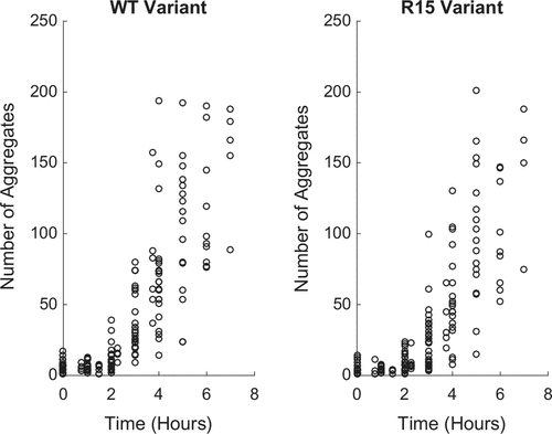
In this work, we consider recent propagon amplification experiments performed on two Sup35 variants which differ in the number of oligopeptide repeats in the prion domain. The variant ‘WT’ represents the wild-type (i.e. standard) version of Sup35 with 5.5 oligopeptide repeats and ‘R15’ which has only the first 5 repeats (i.e. the partial oligopeptide repeat is missing). Both Sup35 variants are capable of forming aggregates and conferring the [$PS{I}^{+}$] prion phenotype. Figure 2 shows the result of experiments on both prion variants. The question we pursue in this analysis is: Are there differences in the rate of aggregate amplification, $\mathit{\lambda }$, between these two variants?

3.2. Growth Rate Distribution Models and Inverse Problem Formulation

In this formulation we make several simplifying assumptions on both the yeast cells and aggregates themselves. While in practice yeast cell division and death rates are time varying, and have been well studied [25,28,29], for simplicity we assume that division rates ${\mathit{\alpha }}_i(t)$ are the same for all cells and generations i (${\mathit{\alpha }}_i(t)=0.0077$ 1/min) and that cell death is negligible, ${\mathit{\beta }}_i(t)=0$. Further, we assume the initial distribution of aggregates to be given by a truncated normal distribution with $\mathit{\mu }=1$ and $\mathit{\sigma }=.1$. The normal distribution is chosen for convenience but is consistent with the initial experimental step where cells are driven to have only a single aggregate (see Figure 1). Finally, while there are two parameters K and $\mathit{\lambda }$ in the logistic model of prion dynamics (see Equation (1(1) $$\begin{array}{c}\hfill \frac{\mathrm{d}y}{\mathrm{d}t}=\frac{\mathit{\lambda }y\left(K-y\right)}{K}:=v(y)\end{array}$$(1) )), because prion curing assays have been used to estimate K, the steady-state number of aggregates in a single cell [7,24,25], we take this value as known ($K=200$) and focus effort on only estimating the growth rate $\mathit{\lambda }$.

Suppose our experimental observations consist of numbers of aggregates ${\{y_i\}}_{i=1}^n$ observed at times ${\{t_i\}}_{i=1}^n$. We assume that these experimentally observed counts reflect the expected number of aggregates in a cell chosen at that time as given below in Equation (11(11) $$\begin{array}{c}\hfill E\left[y(t;\mathit{\lambda })\right]=\frac{{\sum }_{i=0}^{\infty }{\int }_0^{\infty }\mathit{\xi }{N}_i(t,\mathit{\xi };\mathit{\lambda })\mathrm{d}\mathit{\xi }}{N(t)},\end{array}$$(11) )(11) $$\begin{array}{c}\hfill E\left[y(t;\mathit{\lambda })\right]=\frac{{\sum }_{i=0}^{\infty }{\int }_0^{\infty }\mathit{\xi }{N}_i(t,\mathit{\xi };\mathit{\lambda })\mathrm{d}\mathit{\xi }}{N(t)},\end{array}$$(11)

where $N_i(t,\mathit{\xi };\mathit{\lambda })$ is the solution to the aggregate density problem for a given growth rate $\mathit{\lambda }$, number of propagons $\mathit{\xi }$, and generation i since the start of the experiment (see Equation (9(9) $$\begin{array}{c}\hfill \frac{\mathit{\partial }{n}_i(t,y)}{\mathit{\partial }t}+\frac{\mathit{\partial }(f(y)n_i(t,y))}{\mathit{\partial }y}=0\end{array}$$(9) )), and $N(t)={\sum }_{i=0}^{\infty }{\overline{N}}_i(t)$. Rather than go to infinity, the upper limit of the sums is chosen to be the maximum number of generations M chosen based on the length of the experiments. We are interested in estimating the growth rate $\mathit{\lambda }$ in the formulation equation (11(11) $$\begin{array}{c}\hfill E\left[y(t;\mathit{\lambda })\right]=\frac{{\sum }_{i=0}^{\infty }{\int }_0^{\infty }\mathit{\xi }{N}_i(t,\mathit{\xi };\mathit{\lambda })\mathrm{d}\mathit{\xi }}{N(t)},\end{array}$$(11) ). Given a set of observations ${\{y_i\}}_{i=1}^n$ for $E\left[y(t_i;\mathit{\lambda })\right],i=1,\dots ,n$, we are led naturally to an optimization problem(12) $$\begin{array}{c}\hfill \underset{\mathit{\lambda }}{min}{\mathrm{\Sigma }}_{i=1}^n{|E\left[y(t_i;\mathit{\lambda })\right]-y_i|}^2.\end{array}$$(12)

However, we do not expect a single growth rate to suffice for the aggregate type data in which we are interested. To allow for heterogeneity in estimates of the aggregate growth rates, we follow an approach previously used in [30,31] relying on the Porohov Metric (which is equivalent to weak star convergence of measures [32–34]). To this end we assume a family $\mathcal{P}(\mathrm{\Lambda })$ of distributions P of growth rates for our population over a continuum of values $\mathrm{\Lambda }$. We then use the data in a reformulation of the estimation problem(13) $$\begin{array}{c}\hfill P_0=arg\underset{P\in \mathcal{P}(\mathrm{\Lambda })}{min}{J}_{OLS}^n(P)=arg\underset{P\in \mathcal{P}(\mathrm{\Lambda })}{min}{\mathrm{\Sigma }}_{i=1}^n{|E\left[y(t_i;P)\right]-Y_i|}^2,\end{array}$$(13)

where(14) $$\begin{array}{c}\hfill E\left[y(t_i;P)\right]={\int }_{\mathrm{\Lambda }}E\left[y(t_i;\mathit{\lambda })\right]\mathrm{d}P(\mathit{\lambda }).\end{array}$$(14)

Here our formulation assumes that the data $\{y_i\}$ are the realizations for random variable observations $\{Y_i\}$ in an i.i.d. error process given by(15) $$\begin{array}{c}\hfill Y_i=E[y(t_i;P)]+{\mathcal{E}}_i\end{array}$$(15)

where $E[{\mathcal{E}}_i]=0$, and $\text{cov}[{\mathcal{E}}_i,{\mathcal{E}}_i]={\mathit{\sigma }}_0^2$.

In our application here, one can use a continuum of growth rates $\mathrm{\Lambda }=[0,{\mathit{\lambda }}_{max}]$. Since $\mathrm{\Lambda }$ with the Euclidean metric is a compact metric space, then the growth family $\mathcal{P}(\mathrm{\Lambda })$ is a compact metric space when taken with the Prohorov metric [34, p. 173]. Hence, since the least squares cost functional $J_{OLS}^n$ is continuous in P, we are guaranteed the existence of a minimizer in (13(13) $$\begin{array}{c}\hfill P_0=arg\underset{P\in \mathcal{P}(\mathrm{\Lambda })}{min}{J}_{OLS}^n(P)=arg\underset{P\in \mathcal{P}(\mathrm{\Lambda })}{min}{\mathrm{\Sigma }}_{i=1}^n{|E\left[y(t_i;P)\right]-Y_i|}^2,\end{array}$$(13) ) for the given $\{Y_i\}$.

The above problem is an infinite dimensional optimization problem which lends itself to a family of approximation problems. For a given finite family ${\mathrm{\Lambda }}^L=\{{\mathit{\lambda }}_1,{\mathit{\lambda }}_2,\cdots ,{\mathit{\lambda }}_L\}$ of growth rates, we consider approximate families ${\mathcal{P}}^L({\mathrm{\Lambda }}^L)=\{P^L={\mathrm{\Sigma }}_{k=1}^L{p}_k{\mathrm{\Delta }}_{{\mathit{\lambda }}_k}|p_k\ge 0\text{and}{\sum }_{k=1}^L{p}_k=1\}$ where ${\mathrm{\Delta }}_{{\mathit{\lambda }}_k}$ is the Dirac delta distribution with mass at ${\mathit{\lambda }}_k$. We identify the probability distribution $P^L$ with a finite dimensional vector which we denote by the vector ${\overrightarrow{p}}^L=(p_1,\cdots ,p_L)$. The corresponding approximate problems are given by(16) $$\begin{array}{c}\hfill P_0^L=arg\underset{P^L\in {\mathcal{P}}^L({\mathrm{\Lambda }}^L)}{min}{J}_{OLS}^n(P^L)=arg\underset{P^L\in {\mathcal{P}}^L({\mathrm{\Lambda }}^L)}{min}{\mathrm{\Sigma }}_{i=1}^n{|E\left[y(t_i;{\mathrm{\Lambda }}^L,{\overrightarrow{p}}^L)\right]-Y_i|}^2.\end{array}$$(16)

Again, properties of the Prohorov metric [34, p.173] can be used to guarantee the existence of a minimizer $P_0^L$ in (16(16) $$\begin{array}{c}\hfill P_0^L=arg\underset{P^L\in {\mathcal{P}}^L({\mathrm{\Lambda }}^L)}{min}{J}_{OLS}^n(P^L)=arg\underset{P^L\in {\mathcal{P}}^L({\mathrm{\Lambda }}^L)}{min}{\mathrm{\Sigma }}_{i=1}^n{|E\left[y(t_i;{\mathrm{\Lambda }}^L,{\overrightarrow{p}}^L)\right]-Y_i|}^2.\end{array}$$(16) ) for the given data process $\{Y_i\}$.

During the last decade, we have developed a full theoretical framework related to convergence and consistency in problems for the Prohorov metric such as those being discussed here. This theoretical framework, called the Prohorov Metric Framework, or PMF for short, is summarized and discussed in the context of fairly general problems in [34, Chapter 5]. We summarize here portions of the theory that are relevant to our current problems. We first discuss issues related to convergence as $L\to \infty$ of the approximations $P_0^L$ as defined in equation (16(16) $$\begin{array}{c}\hfill P_0^L=arg\underset{P^L\in {\mathcal{P}}^L({\mathrm{\Lambda }}^L)}{min}{J}_{OLS}^n(P^L)=arg\underset{P^L\in {\mathcal{P}}^L({\mathrm{\Lambda }}^L)}{min}{\mathrm{\Sigma }}_{i=1}^n{|E\left[y(t_i;{\mathrm{\Lambda }}^L,{\overrightarrow{p}}^L)\right]-Y_i|}^2.\end{array}$$(16) ) above. These results were first developed in [35] and subsequently used in other problems related to aggregate data.

We let $\mathrm{\Lambda }=[0,{\mathit{\lambda }}_{max}]$ as discussed above and ${\mathrm{\Lambda }}_D={\{{\mathit{\lambda }}_k^D\}}_{k=1}^{\infty }$ be an enumeration of a countable dense subset ${\mathrm{\Lambda }}_D$ of $\mathrm{\Lambda }$. We define $P_D({\mathrm{\Lambda }}_D)$ as the collection of all finite convex combinations ${\mathrm{\Sigma }}_{k=1}^L{p}_k{\mathrm{\Delta }}_{{\mathit{\lambda }}_k}$ of Dirac measures on $\mathrm{\Lambda }$ with atoms ${\mathit{\lambda }}_k^D\in {\mathrm{\Lambda }}_D$ and weights ${\overrightarrow{p}}^L$. Then $P_D({\mathrm{\Lambda }}_D)$ is dense in $P(\mathrm{\Lambda })$. A proof of this result can be found in [35].

For each integer L, we define(17) $$\begin{array}{c}\hfill P_D^L({\mathrm{\Lambda }}_D)=\left\{P^L\in P_D({\mathrm{\Lambda }}_D)|P^L=\sum _{k=1}^L{p}_k{\mathrm{\Delta }}_{{\mathit{\lambda }}_k^D}\right\}.\end{array}$$(17)

That is, for each L, $P_D^L({\mathrm{\Lambda }}_D)$ is the set of all atomic probability measures with nodes placed at the first L elements in the enumeration of the countable dense subset ${\mathrm{\Lambda }}_D$. Note that $P_D^L({\mathrm{\Lambda }}_D)\subset P^L(\mathrm{\Lambda })\subset P(\mathrm{\Lambda })$ for all L. The following theorem provides the desired convergence result.

Theorem 3.1:

There exists a sequence of minimizers $\{P_n^L\}$ of $J_{OLS}^n(P)$ over ${\mathcal{P}}^L(\mathrm{\Lambda })$. Moreover, this sequence has at least one convergent subsequence. The limit $P^{n\ast }$ (as $L\to \infty$) of such a subsequence minimizes $J_{OLS}^n$ over $\mathcal{P}(\mathrm{\Lambda })$.

This theorem follows immediately from the theoretical framework and convergence theorems of [36] and the results above. The power of this theorem is that it transforms an infinite dimensional minimization problem (over $\mathcal{P}(\mathrm{\Lambda })$) into an L dimensional optimization problem. In practice, L nodes ${\{{\mathit{\lambda }}_k^D\}}_{k=1}^L$ from the dense, countable subset ${\mathrm{\Lambda }}_D={\{{\mathit{\lambda }}_k^D\}}_{k=1}^{\infty }$ are fixed in advance and then the L weights $p_k^L$ are estimated in a minimization problem.

We turn next to the question of consistency [34, Section 5.5] which relates to the question of what happens to the minimizer $P^{n\ast }$ of $J_{OLS}^n(P)$ over $\mathcal{P}(\mathrm{\Lambda })$, as $n\to \infty$, (i.e. as an increasing amount of data becomes available). These results, in the context of probability measures, assure us that the measures $P^{n\ast }$ converge in some sense to an underlying ‘true’ probability measure $P_0$. Under appropriate conditions (primarily that the data is collected in a manner that the ‘sampling points fill up the space’ $\mathrm{\Lambda }$ and an additional identifiability assumption), one has (see [34, Theorem 5.5.2]) that the $P^{n\ast }$, as $n\to \infty$, converge with probability 1 to a ‘true’ measure $P_0$. That is, $\text{Prob}\left\{\mathit{\omega }|P^{n\ast }(\mathit{\omega })\to P_0(\mathit{\omega })\right\}=1.$

In the above examples, the formulation of the objectives assumes that the observations $\{Y_i\}$ follow an absolute error model. That is, in an absolute error model we assume that the data, propagon counts $\{y_i\}$, are realizations of observations of the form(18) $$\begin{array}{c}\hfill Y_i=E[y(t_i;{\mathrm{\Lambda }}^L,{\overrightarrow{p}}^L)]+{\mathcal{E}}_i\end{array}$$(18)

where the ${\mathcal{E}}_i$ represent an i.i.d. error process with $E[{\mathcal{E}}_i]=0$, and $\text{cov}[{\mathcal{E}}_i,{\mathcal{E}}_i]={\mathit{\sigma }}_0^2$.

However, because the variance of our data set appeared to increase over time and multiple data points were available at each time (see Figure 2), we considered a proportional error model where the error in the experimental observations is proportional to the expected outcome. In this case, the data $\{y_i\}$ are assumed to be realizations of observations of the form(19) $$\begin{array}{c}\hfill Y_i=E[y(t_i;{\mathrm{\Lambda }}^L,{\overrightarrow{p}}^L)]+E{[y(t_i;{\mathrm{\Lambda }}^L,{\overrightarrow{p}}^L)]}^{\mathit{\delta }}{\mathcal{E}}_i,\text{where}\mathit{\delta }>0.\end{array}$$(19)

As discussed in Appendix 1, we found our fit was best described by a proportional error model with exponent $\mathit{\delta }$ between $0.4-0.7$. For simplicity we chose $\mathit{\delta }=0.4$ in our analysis below, but we note the results were not overly sensitive to this value. With the choice of our proportional error model, we adjust our objective from the OLS to the generalized least squares (GLS) formulation:(20) $$\begin{array}{c}\hfill P_0^L=arg\underset{P^L\in {\mathcal{P}}^L({\mathrm{\Lambda }}^L)}{min}J\left(P^L\right)=argmin\sum _{i=1}^n{\left(\frac{E\left[y(t_i;{\mathrm{\Lambda }}^L,{\overrightarrow{p}}^L)\right]-Y_i}{E{\left[y(t_i;{\mathrm{\Lambda }}^L,{\overrightarrow{p}}^L)\right]}^{\mathit{\delta }}}\right)}^2.\end{array}$$(20)

While the original OLS problem can be readily solved with quadratic programming [37][34], the GLS formulation cannot. In the analysis below we solve our inverse problem by using the Matlab fmincon function and constraining our parameters such that ${\overrightarrow{p}}^L$ satisfies $p_k\ge 0$ and ${\sum }_{k=1}^L{p}_k=1$ for different choices for our possible growth rates.

Before proceeding, we comment further on our choice of statistical model described above. Our present effort represents, to the best of our knowledge, the first attempt to precisely model and quantify propagon counting assays. We believe there are two sources of error in these experiments. First, there is randomness associated with sampling from a population. Second, there is error in the measurements from the final counting which are performed by a human. Our work has demonstrated that there is considerably quantitative power using these assays.

3.3. Inference on simulated data

Before moving to experimental data, we investigated if we could successfully estimate parameters from simulated data-sets. We generated simulated data with the same proportional variance model ($\mathit{\delta }=0.4$) that we chose to use with the experimental data-sets and analysed our ability to correctly predict growth rates under different conditions. In order to maximize consistency between simulations and experiments, we chose the same time points as our experiments and simulated 10 observations at each. We first considered a simulated data-set with a unimodal growth rate distribution where we approximated the normal distribution ($\mathit{\mu }=1.5,\mathit{\sigma }=0.25$) by equally spaced growth rates in the range $\mathrm{\Lambda }=[0.5,2.5]$. We explored our inverse problem formulation varying the number L of nodes in our estimation. The convergence obtained is depicted in Figure 3 and is consistent with that discussed above and illustrated earlier in [37].

Figure 3. Simulated Data with Unimodal Growth Distribution. Each row demonstrates our ability to determine the best fit data to a set of simulated propagon counts with increasing numbers of equally spaced nodes in our discrete model: (Row 1) 5 Nodes, (Row 2) 10 Nodes, (Row 3) 25 Nodes, (Row 4) 50 Nodes and (Row 5) 100 Nodes. In each row we depict: (Left) the simulated propagon counts (black circles) and best fit model output (blue); (Centre) the true probability density (black) compared to estimated probability density (blue) and (Right) the true cumulative distribution (black) compared to estimated cumulative distribution function. We see that with increasing nodes we converge to the cumulative distribution.

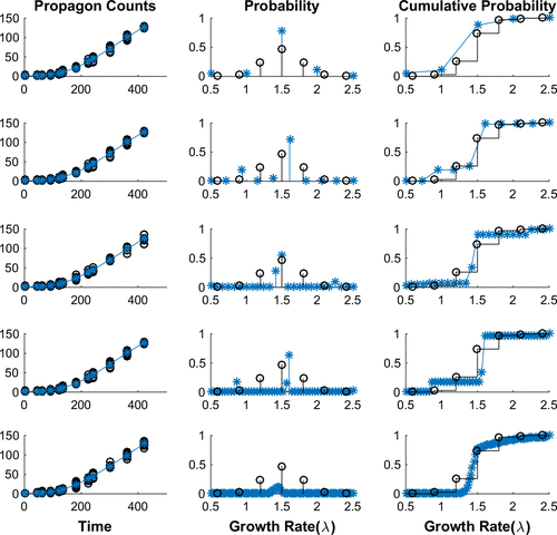
Figure 4. Simulated Data with Bimodal Growth Distribution. Each row demonstrates our ability to determine the best fit data to a set of simulated propagon counts with increasing numbers of equally spaced nodes in our discrete model: (Row 1) 5 Nodes, (Row 2) 10 Nodes, (Row 3) 25 Nodes, (Row 4) 50 Nodes and (Row 5) 100 Nodes. In each row we depict: (Left) the simulated propagon counts (black circles) and best fit model output (blue); (Centre) the true probability density (black) compared to estimated probability density (blue) and (Right) the true cumulative distribution (black) compared to estimated cumulative distribution function. We see that with increasing nodes we converge to the cumulative distribution.

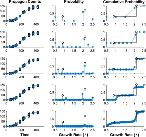
We also generated simulated data with only two nodes: ${\mathit{\lambda }}_{}\text{low}\approx 0.90$, (30% of population), and ${\mathit{\lambda }}_{\text{high}}\approx 2.1$, ($70\%$ of population) and solved inverse problems on the same node sets consisting of $L=5,10,25,50\text{and}100$ equally spaced nodes in [0.5, 2.5] with results be summarized in Figure 4. In all cases the distributions identified in solving the inverse problems were consistent with the true bimodal distribution, although the location of ${\mathit{\lambda }}_{\text{low}}$ was not always correctly predicted. Based on these results, we conclude that the underlying characteristics of the resulting approximations – such as support and modality – in general, are likely to be in agreement with the true bimodal distribution.

4. Parameter inference on experimental data

4.1. Estimating growth rates

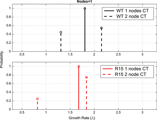
Motivated by our results on simulated data-sets, we formulated and solved inverse problems for our two prion variants WT and R15 (see Figure 2). Using the proportional error model, we identified the optimal discrete probability distribution $\overrightarrow{p}$ for different numbers of equally spaced nodes between 0.5 and 2.5 (see Figures 5–10 solid lines). As the number of nodes increased from 4, we observed bimodality in the probability distribution functions (solid lines) for both WT (black) and R15 (red) variants. Indeed, it seemed that the delta function model was converging for each variant to a bimodal distribution. Based on the results from our simulated data, these estimated node weights appeared consistent with two distinct growth rates rather than a broad unimodal distribution of growth rates.

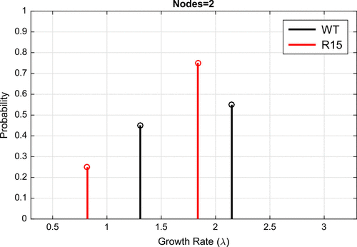
To determine bimodality more directly, we explored an alternative method of parameter estimation by allowing the location of $\mathit{\lambda }$ to vary continuously throughout the interval [0.5, 2.5] and identifying the optimal two node distribution of $\mathit{\lambda }$ (see Figure 11). For reference, we also show the continuously varying values of $\mathit{\lambda }$ and their associated probabilities in dashed lines in Figures 5-10 (dashed lines). Together, the consistent node placement between the continuous and discrete node models suggest that there are two distinct prion aggregate growth rates for WT and R15 variants. Intriguingly, the bimodal behaviour was distinct between variants; assuming cells from the lower and higher $\mathit{\lambda }$ subpopulations are consistent between variants, this suggests an overall higher rate of aggregate amplification for cells with the WT variant compared to the R15 variant (see Figure 11).

Figure 5. 4 Fixed Nodes. Fit to 4 nodes equally spaced in $\mathit{\lambda }=[0.5,2.5].$

Figure 6. 9 Fixed Nodes. Fit to 9 nodes equally spaced in $\mathit{\lambda }=[0.5,2.5].$

Figure 7. 17 Fixed Nodes. Fit to 17 nodes equally spaced in $\mathit{\lambda }=[0.5,2.5].$

Figure 8. 33 Fixed Nodes. Fit to 33 nodes equally spaced in $\mathit{\lambda }=[0.5,2.5].$

Figure 9. 65 Fixed Nodes. Fit to 65 nodes equally spaced in $\mathit{\lambda }=[0.5,2.5].$

Figure 10. 129 Fixed Nodes. Fit to 129 nodes equally spaced in $\mathit{\lambda }=[0.5,2.5].$

Figure 11. Continuously Varying Nodes. Based on the observations for fixed node models, it appeared that the underlying data had a strong preference for two specific nodes.

4.2. Model selection test to assess bimodality

In order to more robustly test the hypothesis of bimodality in the data-sets, we performed a model selection test where we compared our model of two continuously varying values for $\mathit{\lambda }$ with a model where we chose only a single value of $\mathit{\lambda }$. In Figure 12 we compare the location of the best choice for a single node (solid line) with the two node model (dashed lines) for both WT and R15. We note that the optimal single node chosen appears to be close to the weighted average for the two node model. To decide between the one or two growth rate model we performed a model selection test on the residual sum of squares (RSS) for our proportional error model (Equation 20(20) $$\begin{array}{c}\hfill P_0^L=arg\underset{P^L\in {\mathcal{P}}^L({\mathrm{\Lambda }}^L)}{min}J\left(P^L\right)=argmin\sum _{i=1}^n{\left(\frac{E\left[y(t_i;{\mathrm{\Lambda }}^L,{\overrightarrow{p}}^L)\right]-Y_i}{E{\left[y(t_i;{\mathrm{\Lambda }}^L,{\overrightarrow{p}}^L)\right]}^{\mathit{\delta }}}\right)}^2.\end{array}$$(20) ) as described in [34,38,39]. Our statisticcompares the difference between RSS for the one growth rate model ($RS{S}_1$, one parameter $\mathit{\lambda }$) and the RSS for the two growth rate model ($RS{S}_2$, three parameters ${\mathit{\lambda }}_1,{\mathit{\lambda }}_2,p_1$):$$\frac{RS{S}_1-RS{S}_2}{RS{S}_2}\sim {\mathit{\chi }}^2(2).$$

According to the ${\mathit{\chi }}^2$ distribution, there was a significantly better fit for the two node model than the one node model for the WT variant ($p=0.00335$) but not the R15 variant $(p=.1554218)$. However, we note that the R15 data still seem to support the bimodality, otherwise the parameter estimated for the two node model would have converged to the signal node distribution.

Figure 12. 1 vs. 2 Nodes. In order to decide if the underlying data-sets were bimodal, we compare the best bimodal nodes (dashed lines) with the best single node model for each case (WT $=$ black, R15 $=$ red).

4.3. Sensitivity analysis

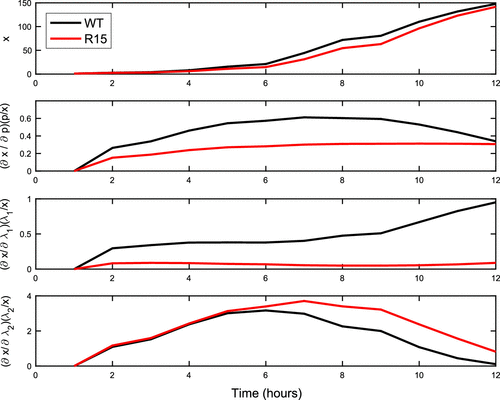
Having strong evidence in support of the two node model for the WT variant and weaker but still suggestive evidence for R15, we analysed the sensitivity of our results to our parameter estimates. Following [39] we used the system of differential equations for the local sensitivity of observed propagon counts to changes from optimal parameters. The sensitivities were computed using the complex-step method [40]. In the analysis below we have chosen to represent the bimodal model with the following three parameters: $p,{\mathit{\lambda }}_1,{\mathit{\lambda }}_2$ where ${\mathit{\lambda }}_1<{\mathit{\lambda }}_2$ and the probability of growth rate ${\mathit{\lambda }}_1$ is p and ${\mathit{\lambda }}_2$ is $(1-p)$.

In Figure 13 we plot the normalized sensitivities in time. We first note that, as expected, the model with R15 parameters has lower predicted aggregate counts than the WT parameters (see Figure 13 (Top)). We note differences in the local sensitivity behaviour of the variants to p and ${\mathit{\lambda }}_1$. The behaviour of WT is increasingly sensitive to p until around 7 h where its sensitivity then begins to decrease in contrast to R15 where sensitivity appears to be slowly increasing then levelling out. Further in comparison to WT, R15 has minimal sensitivity to ${\mathit{\lambda }}_1$. Both WT and R15 exhibit similar behaviour to sensitivities in ${\mathit{\lambda }}_2$ where the sensitivity increases and then decreases after the maximum occurs at around 7 h. We expect strongly decreasing sensitivity to $\mathit{\lambda }$ values as each of the respective subpopulations approach the same aggregate carrying capacity, which likely explains the ${\mathit{\lambda }}_2$ behaviour for both variants.

Figure 13. Time Varying Local Sensitivities. (Top) Model output x for optimal parameter choices. Note that despite the difference in the optimal parameters, the model behaviour for WT (black) and R15 (red) are quite similar. (Second - Bottom) Time varying sensitivities for WT (black) and R15 (red).

4.4. Confidence intervals

We next used our sensitivity matrices (of the previous Section) to estimate confidence intervals for our parameters. We followed the asymptotic theory approach given in [34] for estimating confidence intervals for generalized least squares problems. We first describe F, the sensitivity matrix, which is in this case $12\times 3$ matrix for our 12 time points $\{t_1,t_2,\cdots ,t_{12}\}$ and three parameters. Recall, the output of our model is the expected number of aggregates observed at particular time t. For ease in notation, we redefine our model output for the bimodal case (originally defined in Equation (14(14) $$\begin{array}{c}\hfill E\left[y(t_i;P)\right]={\int }_{\mathrm{\Lambda }}E\left[y(t_i;\mathit{\lambda })\right]\mathrm{d}P(\mathit{\lambda }).\end{array}$$(14) )) as follows:(21) $$\begin{array}{c}\hfill E[t;{\mathit{\lambda }}_1,{\mathit{\lambda }}_2,p]=pE\left[y(t;{\mathit{\lambda }}_1)\right]+(1-p)E\left[y(t;{\mathit{\lambda }}_2)\right].\end{array}$$(21)

The sensitivity matrix is given by(22) $$\begin{array}{c}\hfill F[{\mathit{\lambda }}_1,{\mathit{\lambda }}_2,p]=\left[\begin{array}{ccc}\frac{\mathit{\partial }E[t_1;{\mathit{\lambda }}_1,{\mathit{\lambda }}_2,p]}{\mathit{\partial }p}& \frac{\mathit{\partial }E[t_1;{\mathit{\lambda }}_1,{\mathit{\lambda }}_2,p]}{\mathit{\partial }{\mathit{\lambda }}_1}& \frac{\mathit{\partial }E[t_1;{\mathit{\lambda }}_1,{\mathit{\lambda }}_2,p]}{\mathit{\partial }{\mathit{\lambda }}_2}\\ \cdots & \cdots & \cdots \\ \frac{\mathit{\partial }E[t_{12};{\mathit{\lambda }}_1,{\mathit{\lambda }}_2,p]}{\mathit{\partial }p}& \frac{\mathit{\partial }E[t_{12};{\mathit{\lambda }}_1,{\mathit{\lambda }}_2,p]}{\mathit{\partial }{\mathit{\lambda }}_1}& \frac{\mathit{\partial }E[t_{12};{\mathit{\lambda }}_1,{\mathit{\lambda }}_2,p]}{\mathit{\partial }{\mathit{\lambda }}_2}\\ \end{array}\right]\end{array}$$(22)

Our matrix of weights is given by a proportional variance model, where we chose $\mathit{\delta }=0.4$:(23) $$\begin{array}{c}\hfill W=\text{diag}(E{[t_1;{\mathit{\lambda }}_1,{\mathit{\lambda }}_2,p]}^{2\mathit{\delta }},E{[t_2;{\mathit{\lambda }}_1,{\mathit{\lambda }}_2,p]}^{2\mathit{\delta }}\cdots ,E{[t_{12};{\mathit{\lambda }}_1,{\mathit{\lambda }}_2,p]}^{2\mathit{\delta }}).\end{array}$$(23)

The standard errors of our parameter estimates are given by the square root of the diagonal elements of the covariance matrix $\mathrm{\Sigma }$, where:(24) $$\begin{array}{c}\hfill \mathrm{\Sigma }={\mathit{\sigma }}^2{\left(F^T[{\mathit{\lambda }}_1,{\mathit{\lambda }}_2,p]WF[{\mathit{\lambda }}_1,{\mathit{\lambda }}_2,p]\right)}^{-1}.\end{array}$$(24) (If the precise value of ${\mathit{\sigma }}^2$, the variance of the noise terms in the proportional error model, were known this would be used. Otherwise, as we do in this case, the value ${\mathit{\sigma }}^2$ is estimated from the data.)

Using the formulation above, we computed the standard error and $95\%$ confidence intervals for the WT and R15 parameters (see Tables 1 and 2, respectively). We found greater confidence in our estimated parameters for the WT variant data than those for the R15 data. This is evident in the smaller standard error (SE) and normalized standard error (SE/estimate). A bimodal distribution in growth rates is strongly suggested for the WT variant data because the $95\%$ confidence intervals for ${\mathit{\lambda }}_1$ and ${\mathit{\lambda }}_2$ were disjoint. As we will describe in more detail, the most likely explanation for the two subpopulations in the yeast data is that mother and daughter cells have lower and higher rates of aggregate growth, respectively. Since roughly $40\%$ of the population at steady-state consists of mother cells, the estimate of $p=0.45$ is especially compelling.

For the R15 data, the confidence in our model parameters was lower than that for WT. Of particular concern is the $95\%$ confidence interval for ${\mathit{\lambda }}_1$ not only contains the entire $95\%$ confidence interval for ${\mathit{\lambda }}_2$ but allows for negative growth rates. While based on our inverse problem results, there is support for bimodal growth rates with the R15 variant, our data does not allow us to conclude this with statistical certainty.

Table 1. WT variant – standard error and 95% confidence intervals.

Parameter	Estimate	SE	Normalized SE	Lower Bound	Upper Bound
p	0.45	0.20	0.45	0.06	0.84
${\mathit{\lambda }}_1$	1.31	0.23	0.17	0.86	1.75
${\mathit{\lambda }}_2$	2.15	0.19	0.09	1.78	2.52

Table 2. R15 variant – standard error and 95% confidence intervals.

Parameter	Estimate	SE	Normalized SE	Lower Bound	Upper Bound
p	0.25	0.25	1.00	$-$0.24	0.74
${\mathit{\lambda }}_1$	0.82	2.58	3.15	$-$4.24	5.88
${\mathit{\lambda }}_2$	1.84	0.10	0.06	1.64	2.04

5. Discussion and concluding remarks

Our mathematical model and inverse problem formulation for prion amplification in a yeast colony indicate the possible presence of bimodality in the prion aggregate growth rate distribution. We believe this bimodality is consistent with the underlying asymmetry in the budding yeast reproductive process. When yeast cells divide, the resulting cells are not identical. A daughter grows as a bud on a mature mother cell. When they separate, the daughter cell is smaller and does not inherit the replicative age of the mother. Since previous work has demonstrated a difference in prion aggregate composition between yeast cells in their first generation (daughters) and mature yeast cells (mothers) [15], it is attractive to speculate that these are the same two populations we have identified here. We note that, according to the nucleated polymerization model [11,17], the amount of soluble (healthy) protein directly impacts the aggregate growth rate, so it is possible that differences in the amount of soluble Sup35 in mother and daughter cells could explain this difference.

We note that while our model provides statistical support for bimodality in the aggregate growth rates for the WT variant but not the R15 variant, it is possible that further experimental data might change this conclusion. In addition, we note that there were several simplifying assumptions we made in the analysis of our model that could be revisited. First, our model of cell division considered only exponential cell growth, a more realistic model of yeast cell growth would employ time varying rates of division. Second, our inverse problem formulation considered only heterogeneity in the aggregate growth rates, but we could consider simultaneously estimating growth rates and the aggregate carrying capacity. In future studies we intend to investigate these, and other, extensions.

Acknowledgements

The authors gratefully acknowledge several reviewers whose comments and questions substantially improved the presentation in this manuscript.

Correction Statement

This article has been republished with minor changes. These changes do not impact the academic content of the article.

Additional information

Funding

This research was supported in part by the Air Force Office of Scientific Research [grant number AFOSR FA9550-15-1-0298]; in part by the National Science Foundation under NSF [grant number DMS-0946431], [grant number DMS-1514929], [grant number INSPIRE BCS-13-44279]; in part by the National Institutes of Health [grant number NIGMS R35 GM118042].

Notes

No potential conflict of interest was reported by the authors.

Appendix 1

Fitting proportional error model

Figure A1. Modified Residuals vs. Time for WT data.

Figure A2. Modified Residuals vs. Time for R15 data.

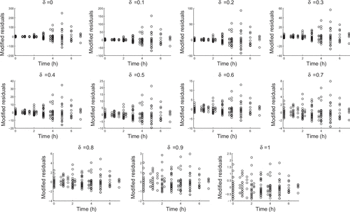
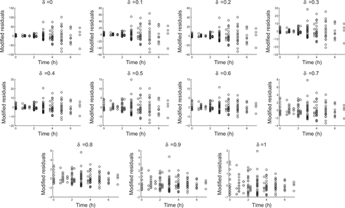
Since our experimental data had multiple observations at each time point, we considered fitting a proportional error model. In Figures A1 and A2 we determined modified residuals by subtractingthe mean of the observed values and dividing by the mean to the appropriate power. That is, if we compute ${\overline{y}}_i$ is the average of all observed counts at the same time, then the modified residuals are:(A1) $$\begin{array}{c}\hfill M(y_i)=\frac{y_i-{\overline{y}}_i}{{\overline{y}}_i^{\mathit{\delta }}}.\end{array}$$(A1)

In a proportional error model, we would expect the residuals to be uniformly dispersed at $\mathit{\delta }=0$. However, we see that the data are more consistent with $\mathit{\delta }>0$ as dispersal increases with nonzero $\mathit{\delta }$. In the analysis of our data we chose the value $\mathit{\delta }=0.4$ but the results were consistent for $\mathit{\delta }$ values between 0.4 and 0.6.

References

- Knowles TPJ , Vendruscolo M , Dobson CM . The amyloid state and its association with protein misfolding diseases. Nat Rev Mol Cell Biol. 2014;15(6):384–396.
- Aguzzi A , Polymenidou M . Mammalian prion biology: one century of evolving concepts. Cell. 2004;116(2):313–327.
- Collinge J . Prion diseases of humans and animals: their causes and molecular basis. Ann Rev Neurosci. 2001;24(1):519–550.
- Sindi SS , Serio TR . Prion dynamics and the quest for the genetic determinant in protein-only inheritance. Curr Opin Microbiol. 2009;12(6):623–630.
- Tuite MF , Serio TR . The prion hypothesis: from biological anomaly to basic regulatory mechanism. Nat Rev Mol Cell Biol. 2010;11(12):823–833.
- Palmer KJ , Ridout MS , Morgan BJT . Kinetic models of guanidine hydrochloride-induced curing of the yeast [psi+] prion. J Theor Biol. 2011;274(1):1–11.
- Olofsson P , Sindi SS . A crump-mode-jagers branching process model of prion loss in yeast. J Appl Probab. 2014;51(2):453–465.
- Ridout M , Giagos V , Morgan B , et al. Modelling prion dynamics in yeast. International Statistical Institute Proceedings of the 58th World Statistical Congress, Dublin (Session IPS020). 2011.
- Pöschel T , Brilliantov NV , Frömmel C . Kinetics of prion growth. Biophys J. 2003;85(6):3460–3474.
- Greer ML , Pujo-Menjouet L , Webb GF . A mathematical analysis of the dynamics of prion proliferation. J Theor Biol. 2006;242(3):598–606.
- Davis JK , Sindi SS . A mathematical model of the dynamics of prion aggregates with chaperone-mediated fragmentation. J Math Biol. 2016;72(6):1555–1578.
- Prüss J , Pujo-Menjouet L , Webb G , et al . Analysis of a model for the dynamics of prions. Discrete Contin Dyn Syst Ser B. 2006;6(1):225–235.
- Engler H , Prüss J , Webb GF . Analysis of a model for the dynamics of prions ii. J Math Anal Appl. 2006;324(1):98–117.
- Tanaka M , Collins SR , Toyama BH , et al . The physical basis of how prion conformations determine strain phenotypes. Nature. 2006;442(7102):585–589.
- Derdowski A , Sindi SS , Klaips CL , et al . A size threshold limits prion transmission and establishes phenotypic diversity. Science. 2010;330(6004):680–683.
- Klaips CL , Hochstrasser ML , Langlois CR , et al. Spatial quality control bypasses cell-based limitations on proteostasis to promote prion curing. eLife. 2014;3:e04288
- Masel J , Jansen VAA , Nowak MA . Quantifying the kinetic parameters of prion replication. Biophys Chem. 1999;77(2):139–152.
- Davis JK , Sindi SS . A study in nucleated polymerization models of protein aggregation. Appl Math Lett. 2015;40:97–101.
- Calvez V , Lenuzza N , Doumic M , et al . Prion dynamics with size dependency-strain phenomena. J Biol Dyn. 2010;4(1):28–42.
- Banks HT , Flores KB , Sindi SS . On analytical and numerical approaches to division and label structured population models. Appl Math Lett. 2016;60:81–88.
- Banks HT , Sutton KL , Thompson WC , et al . Estimation of cell proliferation dynamics using cfse data. Bull Math Biol. 2011;73(1):116–150.
- Thompson WC . Partial differential equation modeling of flow cytometry data from CFSE-based proliferation assays. Raleigh (NC): North Carolina State University; 2011.
- Hasenauer J , Schittler D , Allgöwer F . Analysis and simulation of division-and label-structured population models. Bull Math Biol. 2012;74(11):2692–2732.
- Cole DJ , Morgan BJT , Ridout MS , et al . Estimating the number of prions in yeast cells. Math Med Biol. 2004;21(4):369–395.
- Byrne LJ , Cole DJ , Cox BS , et al . The number and transmission of [psi+] prion seeds (propagons) in the yeast saccharomyces cerevisiae. PLoS One. 2009;4(3):e4670–e4670.
- Byrne LJ , Cox BS , Cole DJ , et al . Cell division is essential for elimination of the yeast [psi+] prion by guanidine hydrochloride. Proc Nat Acad Sci. 2007;104(28):11688–11693.
- Langlois CR , Pei F , Sindi SS , et al . Distinct prion domain sequences ensure efficient amyloid propagation by promoting chaperone binding or processing In vivo. In Review.
- Cipollina C , Vai M , Porro D , et al . Towards understanding of the complex structure of growing yeast populations. J Biotechnol. 2007;128(2):393–402.
- Gyllenberg M . The size and scar distributions of the yeast saccharomyces cerevisiae. J Math Biol. 1986;24(1):81–101.
- Banks HT , Fitzpatrick BG . Estimation of growth rate distributions in size structured population models. Q Appl Math. 1991;49:215–235.
- Banks HT , Fitzpatrick BG , Potter Y , et al . Estimation of probability distributions for individual parameters using aggregate population data. Stochastic analysis, control, optimization and applications. Springer; 1999. p. 353–371.
- Billingsley P . Convergence of probability measures. Wiley; 2013.
- Banks HT . A functional analysis framework for modeling, estimation and control in science and engineering. CRC Press; 2012.
- Banks HT , Hu S , Thompson WC . Modeling and inverse problems in the presence of uncertainty. CRC Press; 2014.
- Banks HT , Bihari KL . Modeling and estimating uncertainty in parameter estimation. Inverse Prob. 2001;17:95–111.
- Banks HT , Kunisch Karl . Estimation techniques for distributed parameter systems. Boston (MA): Birkhausen; 1989.
- Banks HT , Davis JL . A comparison of approximation methods for the estimation of probability distributions on parameters. Appl Numer Math. 2007;57(5):753–777.
- Banks HT , Fitzpatrick BG . Statistical methods for model comparison in parameter estimation problems for distributed systems. J Math Biol. 1990;28(5):501–527.
- Banks HT , Tran HT . Mathematical and experimental modeling of physical and biological processes. CRC Press; 2009.
- Martins JRRA , Kroo IM , Alonso JJ . An automated method for sensitivity analysis using complex variables. AIAA paper 2000–0689, 38th Aerospace Sciences Meeting. Reno (NC); 2000. p. 2000–0689.