A harmonic -based conductivity reconstruction method in MREIT with influence of non-transversal current density

Abstract

Magnetic resonance electrical impedance tomography (MREIT) is a high-resolution conductivity imaging method utilizing measured magnetic flux density data induced by externally injected currents. Most MREIT image reconstruction methods including the harmonic $B_z$ algorithm adopt iterative schemes to handle the non-linear relation between conductivity and magnetic flux density. Iterative methods, however, may not guarantee a reliable conductivity reconstruction when the measured magnetic flux density data are contaminated with a significant amount of noise. In this paper, we propose a new image reconstruction method which alleviates the technical difficulties of the iterative harmonic $B_z$ algorithm. It effectively reduces the number of iterations by two at most. To improve the image quality, it incorporates the influence of non-transversal current densities. Providing theoretical observations and details of the proposed algorithm, we present results of numerical simulations and phantom experiments for its validation.

Keywords:

• MREIT
• $B_z$-based algorithm
• conductivity and current density reconstruction
• non-transversal current density
• phantom experiment

1. Introduction

There have been numerous studies to develop electrical conductivity imaging techniques for clinical applications for the last three decades [1,2]. By injecting currents and measuring induced voltages using surface electrodes, electrical impedance tomography (EIT) visualizes distributions of electrical conductivity and permittivity inside the human body [3]. EIT is advantageous as a real-time functional imaging method with a high-temporal resolution where changes of internal conductivity distributions are continuously monitored. Its spatial resolution is, however, much lower than those of other imaging modalities such as magnetic resonance imaging, X-ray computerized tomography and ultrasound imaging, since the spatial resolution depends on the number of electrodes and the image reconstruction problem is a severely ill-posed inverse problem.

Magnetic resonance electrical impedance tomography (MREIT) has been developed as a static conductivity imaging method with a high-spatial resolution. It resolves the uncertainty in internal current pathways by utilizing the measured internal data of induced magnetic flux density [4–19]. Assuming that the conductivity distribution $\mathit{\sigma }:=\mathit{\sigma }(x,y,z)$ is isotropic, the relation between the conductivity and the electrical potential $u:=u(x,y,z)$ can be described by the following second-order elliptic boundary value problem:(1.1) $$\begin{array}{c}\hfill \left\{\begin{array}{c}\mathrm{\nabla }·\mathit{\sigma }\mathrm{\nabla }u=0\text{in}\mathrm{\Omega },\hfill \\ I={\int }_{{\mathcal{E}}^{+}}\mathit{\sigma }\mathrm{\nabla }u·\mathbf{n}\mathrm{d}s,=-{\int }_{{\mathcal{E}}^{-}}\mathit{\sigma }\mathrm{\nabla }u·\mathbf{n}\mathrm{d}s,\hfill \\ {\mathit{\sigma }\mathrm{\nabla }u\times \mathbf{n}|}_{{\mathcal{E}}^{+}\cup {\mathcal{E}}^{-}}=0,\hfill \\ \mathit{\sigma }\mathrm{\nabla }u·\mathbf{n}=0\text{on}\mathit{\partial }\mathrm{\Omega }\backslash \overline{{\mathcal{E}}^{+}\cup {\mathcal{E}}^{-}},\hfill \end{array}\right.\end{array}$$(1.1)

where $\mathrm{\Omega }$ is a given imaging domain in ${\mathbb{R}}^3$ and I is the amplitude of the injected current between a chosen electrode pair ${\mathcal{E}}^{\pm }$. The internal current density $\mathbf{J}=(J_x,J_y,J_z)$ is given by(1.2) $$\begin{array}{c}\hfill \mathbf{J}=-\mathit{\sigma }\mathrm{\nabla }u.\end{array}$$(1.2)

The harmonic $B_z$ algorithm reconstructs conductivity images using measured data of $B_z$ which is the z-component of the magnetic flux density $\mathbf{B}=(B_x,B_y,B_z)$ [20–22]. It has been used in experimental MREIT studies, since it does not require the imaging object to be rotated to measure $B_x$ and $B_y$ in addition to $B_z$. Since $\mathrm{\nabla }·\mathbf{B}=0$, the following identity provides the relation among the conductivity, current density and magnetic flux density [2]:(1.3) $$\begin{array}{c}\hfill \mathbf{J}\times \mathrm{\nabla }ln\mathit{\sigma }=\frac{1}{{\mathit{\mu }}_0}{\mathrm{\nabla }}^2\mathbf{B},\end{array}$$(1.3)

where ${\mathit{\mu }}_0$ is the magnetic permeability of the free space. Two independent injection currents between two different pairs of electrodes as shown in Figure 1 induce magnetic flux densities $B_{z,1}$ and $B_{z,2}$ corresponding to current densities ${\mathbf{J}}_1$ and ${\mathbf{J}}_2$, respectively. Then, the relation in (1.3(1.3) $$\begin{array}{c}\hfill \mathbf{J}\times \mathrm{\nabla }ln\mathit{\sigma }=\frac{1}{{\mathit{\mu }}_0}{\mathrm{\nabla }}^2\mathbf{B},\end{array}$$(1.3) ) is expanded as(1.4) $$\begin{array}{c}\hfill {\mathrm{\nabla }}_{xy}ln\mathit{\sigma }=\frac{1}{{\mathit{\mu }}_0}{\mathbf{A}}^{-1}\left(\begin{array}{c}{\mathrm{\nabla }}^2{B}_{z,1}\\ {\mathrm{\nabla }}^2{B}_{z,2}\end{array}\right),\end{array}$$(1.4)

where ${\mathrm{\nabla }}_{xy}=\left(\frac{\mathit{\partial }}{\mathit{\partial }x},\frac{\mathit{\partial }}{\mathit{\partial }y}\right)$ and$$\begin{array}{c}\hfill \mathbf{A}=\left(\begin{array}{cc}-J_{y,1}& J_{x,1}\\ -J_{y,2}& J_{x,2}\end{array}\right).\end{array}$$

Because of the nonlinearity between $\mathbf{A}$ and $\mathit{\sigma }$, the harmonic $B_z$ algorithm iteratively updates the conductivity and current densities using (1.1(1.1) $$\begin{array}{c}\hfill \left\{\begin{array}{c}\mathrm{\nabla }·\mathit{\sigma }\mathrm{\nabla }u=0\text{in}\mathrm{\Omega },\hfill \\ I={\int }_{{\mathcal{E}}^{+}}\mathit{\sigma }\mathrm{\nabla }u·\mathbf{n}\mathrm{d}s,=-{\int }_{{\mathcal{E}}^{-}}\mathit{\sigma }\mathrm{\nabla }u·\mathbf{n}\mathrm{d}s,\hfill \\ {\mathit{\sigma }\mathrm{\nabla }u\times \mathbf{n}|}_{{\mathcal{E}}^{+}\cup {\mathcal{E}}^{-}}=0,\hfill \\ \mathit{\sigma }\mathrm{\nabla }u·\mathbf{n}=0\text{on}\mathit{\partial }\mathrm{\Omega }\backslash \overline{{\mathcal{E}}^{+}\cup {\mathcal{E}}^{-}},\hfill \end{array}\right.\end{array}$$(1.1) ) and (1.4(1.4) $$\begin{array}{c}\hfill {\mathrm{\nabla }}_{xy}ln\mathit{\sigma }=\frac{1}{{\mathit{\mu }}_0}{\mathbf{A}}^{-1}\left(\begin{array}{c}{\mathrm{\nabla }}^2{B}_{z,1}\\ {\mathrm{\nabla }}^2{B}_{z,2}\end{array}\right),\end{array}$$(1.4) ). This iterative process, however, may fail in experimental studies due to measurement noise and artefacts [23–25]. In addition, the matrix $\mathbf{A}$ becomes near singular at the internal boundary of large conductivity contrast, since ${\mathbf{J}}_1$ and ${\mathbf{J}}_2$ become almost parallel at such boundary region. Under these circumstances, $\mathbf{A}$ becomes more ill-conditioned as the number of iterations increases.

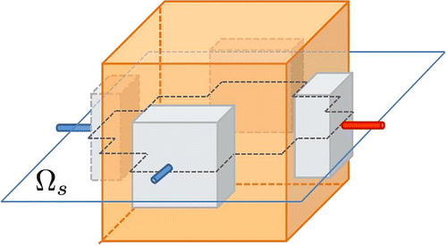
In [26], a non-iterative conductivity and current density image reconstruction method was developed for a cylindrical imaging object. We denote a two-dimensional slice of a rectangular (or cylindrical) domain at $z=s$ by ${\mathrm{\Omega }}_s$; see Figure 1. If the current density is transversally dominant on the imaging plane ${\mathrm{\Omega }}_s$, we can recover the transversal current density ${\mathbf{J}}_{xy}^{\text{rec}}$ from ${\mathrm{\nabla }}^2{B}_z$. Substituting the entries of ${\mathbf{J}}_{xy}^{\text{rec}}$ into the matrix $\mathbf{A}$, we can directly reconstruct the conductivity from (1.4(1.4) $$\begin{array}{c}\hfill {\mathrm{\nabla }}_{xy}ln\mathit{\sigma }=\frac{1}{{\mathit{\mu }}_0}{\mathbf{A}}^{-1}\left(\begin{array}{c}{\mathrm{\nabla }}^2{B}_{z,1}\\ {\mathrm{\nabla }}^2{B}_{z,2}\end{array}\right),\end{array}$$(1.4) ). In [27], a different non-iterative algorithm was proposed based on the definition of a projected current density. These methods, however, fail when the current density is not transversally dominant.

Figure 1. Rectangular domain with two pairs of attached electrodes.

In this paper, an improved harmonic $B_z$ algorithm is proposed to reduce the number of iterations while including the influence of the non-transversal current density. To reduce the number of iterations by two at most, the current density decomposition method in [26–28] is adopted. The current density $\mathbf{J}$ is expressed as a sum of ${\mathbf{J}}_{xy}^0$ and ${\mathbf{J}}_{xy}^{\ast }$. Here, ${\mathbf{J}}_{xy}^0$ is a transversal component of the current density in the presumed homogeneous imaging domain subject to the same injection current. The other transversal component ${\mathbf{J}}_{xy}^{\ast }$ can be obtained using the measured $B_z$ data and the computed non-transversal component $J_z^0$ in the homogeneous domain. To incorporate the local influence of the non-transversal current density $J_z$, a two-step approach is proposed. To implement the proposed two-step $B_z$ algorithm, the three-dimensional forward problem is modified to avoid the impractical boundary condition in [27,28] and the difficulty in estimating the amount of current density on the imaging plane in [26]. We will first provide mathematical observations to establish the validity of the proposed algorithm. After introducing the two-step algorithm, we will present results of numerical simulations and phantom experiments.

2. Preliminary

This section briefly revisits the previous study in [26]. The mathematical observation in [26] showed that the difference between the true and reconstructed transversal current densities depends on the z-component of the true current density $\mathbf{J}$. More precisely, in a given imaging slice ${\mathrm{\Omega }}_s$, we first solve the following second-order elliptic problems for $\mathrm{\Psi }$ and $\mathit{\varphi }$:$$\begin{array}{c}\hfill \left\{\begin{array}{cc}{\mathrm{\nabla }}^2\mathrm{\Psi }=0\hfill & \text{in}{\mathrm{\Omega }}_s,\hfill \\ \mathrm{\nabla }\mathrm{\Psi }·\mathbf{n}=0\hfill & \text{on}\mathit{\partial }{\mathrm{\Omega }}_s\cap \left({\mathcal{E}}^{+}\cup {\mathcal{E}}^{-}\right),\hfill \\ \mathrm{\Psi }=\pm 1\hfill & \text{on}\mathit{\partial }{\mathrm{\Omega }}_s\backslash {\mathcal{E}}^{\pm }\hfill \end{array}\right.\end{array}$$

and$$\begin{array}{c}\hfill \left\{\begin{array}{cc}{\mathrm{\nabla }}^2\mathit{\varphi }=\frac{1}{{\mathit{\mu }}_0}{\mathrm{\nabla }}^2{B}_z\hfill & \text{in}{\mathrm{\Omega }}_s,\hfill \\ \mathrm{\nabla }\mathit{\varphi }·\mathbf{n}=0\hfill & \text{on}\mathit{\partial }{\mathrm{\Omega }}_s\cap \left({\mathcal{E}}^{+}\cup {\mathcal{E}}^{-}\right),\hfill \\ \mathit{\varphi }=0\hfill & \text{on}\mathit{\partial }{\mathrm{\Omega }}_s\backslash {\mathcal{E}}^{\pm }.\hfill \end{array}\right.\end{array}$$

We determine the scaling coefficient $\mathit{\beta }$ by the following relation [26]:$$\begin{array}{c}\hfill \mathit{\beta }=\left(-{\int }_{{\mathcal{E}}^{+}\cap \mathit{\partial }{\mathrm{\Omega }}_s}{\mathbf{J}}_{xy}·\mathbf{n}\mathrm{d}s-{\int }_{{\mathcal{E}}^{+}\cap \mathit{\partial }{\mathrm{\Omega }}_s}{\mathrm{\nabla }}_{xy}\mathit{\varphi }\times \mathbf{n}\mathrm{d}s\right)/\left({\int }_{{\mathcal{E}}^{+}\cap \mathit{\partial }{\mathrm{\Omega }}_s}{\mathrm{\nabla }}_{xy}\mathrm{\Psi }\times \mathbf{n}\mathrm{d}s\right).\end{array}$$

Then, we have(2.1) $$\begin{array}{c}\hfill {\int }_{{\mathrm{\Omega }}_s}{\left|{\mathbf{J}}_{xy}+\left(\mathit{\beta }{\mathrm{\nabla }}_{xy}^{\perp }\mathrm{\Psi }+{\mathrm{\nabla }}_{xy}^{\perp }\mathit{\varphi }\right)\right|}^2\mathrm{d}x\mathrm{d}y\le C{\int }_{{\mathrm{\Omega }}_s}{\left|\frac{\mathit{\partial }}{\mathit{\partial }z}{J}_z\right|}^2\mathrm{d}x\mathrm{d}y,\end{array}$$(2.1)

where C is a positive constant depending only on ${\mathrm{\Omega }}_s$. Note that ${\mathrm{\nabla }}_{xy}^{\perp }=\left(-\frac{\mathit{\partial }}{\mathit{\partial }y},\frac{\mathit{\partial }}{\mathit{\partial }x}\right)$.

Assuming $\frac{\mathit{\partial }}{\mathit{\partial }z}{J}_z\approx 0$, one may reconstruct the transversal current density by (2.1(2.1) $$\begin{array}{c}\hfill {\int }_{{\mathrm{\Omega }}_s}{\left|{\mathbf{J}}_{xy}+\left(\mathit{\beta }{\mathrm{\nabla }}_{xy}^{\perp }\mathrm{\Psi }+{\mathrm{\nabla }}_{xy}^{\perp }\mathit{\varphi }\right)\right|}^2\mathrm{d}x\mathrm{d}y\le C{\int }_{{\mathrm{\Omega }}_s}{\left|\frac{\mathit{\partial }}{\mathit{\partial }z}{J}_z\right|}^2\mathrm{d}x\mathrm{d}y,\end{array}$$(2.1) ), that is,(2.2) $$\begin{array}{c}\hfill {\mathbf{J}}_{xy}\approx {\mathbf{J}}_{xy}^{\text{rec}}:=-\mathit{\beta }{\mathrm{\nabla }}_{xy}^{\perp }\mathrm{\Psi }-{\mathrm{\nabla }}_{xy}^{\perp }\mathit{\varphi }.\end{array}$$(2.2)

However, the current density may not be restricted in the transversal plane even if the imaging object is a rectangular or cylindrical domain, since the current density depends on the internal conductivity distribution. The estimation of $\mathit{\beta }$ in ${\mathrm{\Omega }}_s$ seems to be impossible in experiments, since we only know the total amount of injected current in the whole domain $\mathrm{\Omega }$. However, (2.1(2.1) $$\begin{array}{c}\hfill {\int }_{{\mathrm{\Omega }}_s}{\left|{\mathbf{J}}_{xy}+\left(\mathit{\beta }{\mathrm{\nabla }}_{xy}^{\perp }\mathrm{\Psi }+{\mathrm{\nabla }}_{xy}^{\perp }\mathit{\varphi }\right)\right|}^2\mathrm{d}x\mathrm{d}y\le C{\int }_{{\mathrm{\Omega }}_s}{\left|\frac{\mathit{\partial }}{\mathit{\partial }z}{J}_z\right|}^2\mathrm{d}x\mathrm{d}y,\end{array}$$(2.1) ) is a noble estimation for the reconstructed current density, which leads to improved reconstructions without iterations. In the next section, we will suggest how to reduce the right-hand side of (2.1(2.1) $$\begin{array}{c}\hfill {\int }_{{\mathrm{\Omega }}_s}{\left|{\mathbf{J}}_{xy}+\left(\mathit{\beta }{\mathrm{\nabla }}_{xy}^{\perp }\mathrm{\Psi }+{\mathrm{\nabla }}_{xy}^{\perp }\mathit{\varphi }\right)\right|}^2\mathrm{d}x\mathrm{d}y\le C{\int }_{{\mathrm{\Omega }}_s}{\left|\frac{\mathit{\partial }}{\mathit{\partial }z}{J}_z\right|}^2\mathrm{d}x\mathrm{d}y,\end{array}$$(2.1) ). We will adopt the three-dimensional problem to estimate the scaling coefficient $\mathit{\beta }$ more accurately.

3. Two-step $B_z$ algorithm with an influence of non-transversal current density

The domain $\mathrm{\Omega }$ is assumed to be rectangular and consists of imaging slices ${\mathrm{\Omega }}_s$ such as $\mathrm{\Omega }={\cup }_s{\mathrm{\Omega }}_s$. The Hilbert space $H_k(\mathrm{\Omega })$ is a set of all functions on the domain $\mathrm{\Omega }$ that are square integrable up to the k-th derivative and its norm is denoted by${\Vert ·\Vert }_{H_k(\mathrm{\Omega })}$. Note that $H_0=L_2$ and ${\Vert \mathbf{u}\Vert }_{{\mathbf{L}}^2(\mathrm{\Omega })}$ is the Euclidean norm of the vector $\mathbf{u}$. Two vector functions ${\mathbf{J}}_{xy}^0$ and ${\mathbf{J}}_{xy}^{\ast }$ are considered to approximate the transversal component ${\mathbf{J}}_{xy}$ of $\mathbf{J}$. Here, ${\mathbf{J}}_{xy}^0$ is the transversal current density in $\mathrm{\Omega }$ with the presumed homogeneous conductivity distribution for the same injection current. Note that ${\mathbf{J}}_{xy}^{\ast }$ represents the local correction of the transversal current density using ${\mathrm{\nabla }}^2{B}_z$ and $J_z$ of $\mathbf{J}$. Then, ${\mathbf{J}}_{xy}^0+{\mathbf{J}}_{xy}^{\ast }$ is an approximated transversal current density including the influence of $J_z$ or $\frac{\mathit{\partial }}{\mathit{\partial }z}{J}_z$ of $\mathbf{J}$. The two-step $B_z$ algorithm is based on the following observation.

Observation 3.1:

Let $\mathbf{J}\in {\left[H_1(\mathrm{\Omega })\right]}^3$ be a given current density distribution satisfying (1.2(1.2) $$\begin{array}{c}\hfill \mathbf{J}=-\mathit{\sigma }\mathrm{\nabla }u.\end{array}$$(1.2) ) with (1.1(1.1) $$\begin{array}{c}\hfill \left\{\begin{array}{c}\mathrm{\nabla }·\mathit{\sigma }\mathrm{\nabla }u=0\text{in}\mathrm{\Omega },\hfill \\ I={\int }_{{\mathcal{E}}^{+}}\mathit{\sigma }\mathrm{\nabla }u·\mathbf{n}\mathrm{d}s,=-{\int }_{{\mathcal{E}}^{-}}\mathit{\sigma }\mathrm{\nabla }u·\mathbf{n}\mathrm{d}s,\hfill \\ {\mathit{\sigma }\mathrm{\nabla }u\times \mathbf{n}|}_{{\mathcal{E}}^{+}\cup {\mathcal{E}}^{-}}=0,\hfill \\ \mathit{\sigma }\mathrm{\nabla }u·\mathbf{n}=0\text{on}\mathit{\partial }\mathrm{\Omega }\backslash \overline{{\mathcal{E}}^{+}\cup {\mathcal{E}}^{-}},\hfill \end{array}\right.\end{array}$$(1.1) ) and ${\mathbf{J}}^0\in {\left[H_1(\mathrm{\Omega })\right]}^3$ be the gradient of $\mathit{\psi }$ which satisfies the following elliptic problem:(3.1) $$\begin{array}{c}\hfill \left\{\begin{array}{cc}{\mathrm{\nabla }}^2\mathit{\psi }=0\hfill & \text{in}\mathrm{\Omega },\hfill \\ \mathrm{\nabla }\mathit{\psi }·\mathbf{n}=\mathbf{J}·\mathbf{n}\hfill & \text{on}{\mathcal{E}}^{\pm },\hfill \\ \mathrm{\nabla }\mathit{\psi }·\mathbf{n}=0\hfill & \text{on}\mathit{\partial }\mathrm{\Omega }\backslash {\mathcal{E}}^{\pm }.\hfill \end{array}\right.\end{array}$$(3.1)

Let ${\widehat{J}}_z$ be any function in $H_1(\mathrm{\Omega })$ which satisfies(3.2) $$\begin{array}{c}\hfill {\int }_{{\mathrm{\Omega }}_s}\frac{\mathit{\partial }}{\mathit{\partial }z}\left({\widehat{J}}_z-J_z^0\right)\mathrm{d}x\mathrm{d}y=0\end{array}$$(3.2)

and ${\mathbf{J}}_{xy}^{\ast }\in {\left[H_1({\mathrm{\Omega }}_s)\right]}^2$ be a solution of(3.3) $$\begin{array}{c}\hfill \left\{\begin{array}{cc}{\mathrm{\nabla }}_{xy}·{\mathbf{J}}_{xy}^{\ast }=-\frac{\mathit{\partial }}{\mathit{\partial }z}\left({\widehat{J}}_z-J_z^0\right)\hfill & \text{in}{\mathrm{\Omega }}_s,\hfill \\ {\mathrm{\nabla }}_{xy}^{\perp }·{\mathbf{J}}_{xy}^{\ast }=-\frac{1}{{\mathit{\mu }}_0}{\mathrm{\nabla }}^2{B}_z\hfill & \text{in}{\mathrm{\Omega }}_s,\hfill \\ {\mathbf{J}}_{xy}^{\ast }·\mathbf{n}=0\hfill & \text{on}\mathit{\partial }{\mathrm{\Omega }}_s.\hfill \end{array}\right.\end{array}$$(3.3)

Then, there exists a positive constant C such that$$\begin{array}{c}\hfill {\int }_{{\mathrm{\Omega }}_s}{\left|{\mathbf{J}}_{xy}-\left({\mathbf{J}}_{xy}^0+{\mathbf{J}}_{xy}^{\ast }\right)\right|}^2\mathrm{d}x\mathrm{d}y\le C{\int }_{{\mathrm{\Omega }}_s}{\left|\frac{\mathit{\partial }}{\mathit{\partial }z}\left(J_z-{\widehat{J}}_z\right)\right|}^2\mathrm{d}x\mathrm{d}y.\end{array}$$

Figure 2. Computational setup. (a) Box-shaped domain with four electrodes. (b) Illustration of the conductivity distribution. (c) Triangulation.

Figure 3. Conductivity images in the centre slice: low contrast case. (a) True conductivity distribution. (b) Reconstructed conductivity image without considering the influence of $J_z$ component. (c) Reconstructed conductivity image using the two-step algorithm considering the influence of $J_z$ component. (d) and (e) are one-dimensional profiles along $x=64$ and $y=50$, respectively. Red, green and blue lines are from (a), (b) and (c), respectively. Note that blue lines are much closer to red lines.

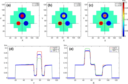
Figure 4. Relative $L_2$ error plots in three regions of interest (ROI): low contrast case. (a) shows the selected ROIs. (b), (c) and (d) are the relative $L_2$ error plots for the red, blue and green ROIs, respectively.

Proof See Appendix A.1.

Remark 3.2:

In the above observation, we use the normal vector $\mathbf{n}$ on the boundary for both two and three dimensions since $\mathbf{n}=(n_x,n_y,0)$.

Remark 3.3:

The planar div–curl system (3.3(3.3) $$\begin{array}{c}\hfill \left\{\begin{array}{cc}{\mathrm{\nabla }}_{xy}·{\mathbf{J}}_{xy}^{\ast }=-\frac{\mathit{\partial }}{\mathit{\partial }z}\left({\widehat{J}}_z-J_z^0\right)\hfill & \text{in}{\mathrm{\Omega }}_s,\hfill \\ {\mathrm{\nabla }}_{xy}^{\perp }·{\mathbf{J}}_{xy}^{\ast }=-\frac{1}{{\mathit{\mu }}_0}{\mathrm{\nabla }}^2{B}_z\hfill & \text{in}{\mathrm{\Omega }}_s,\hfill \\ {\mathbf{J}}_{xy}^{\ast }·\mathbf{n}=0\hfill & \text{on}\mathit{\partial }{\mathrm{\Omega }}_s.\hfill \end{array}\right.\end{array}$$(3.3) ) has a unique solution if ${\mathrm{\Omega }}_s$ is bounded, $\mathit{\partial }{\mathrm{\Omega }}_s$ is a closed $C^{1,1}$ curve, $\frac{\mathit{\partial }}{\mathit{\partial }z}\left({\widehat{J}}_z-J_z^0\right)\in L^p({\mathrm{\Omega }}_s)$ with ${\int }_{{\mathrm{\Omega }}_s}\frac{\mathit{\partial }}{\mathit{\partial }z}\left({\widehat{J}}_z-J_z^0\right)\mathrm{d}x\mathrm{d}y=0$, and $\frac{1}{{\mathit{\mu }}_0}{\mathrm{\nabla }}^2{B}_z\in L^p({\mathrm{\Omega }}_s)$ for $p>1$ [29].

Remark 3.4:

In [27], the projected current density was generated with ${\mathbf{J}}^0$ from (3.1(3.1) $$\begin{array}{c}\hfill \left\{\begin{array}{cc}{\mathrm{\nabla }}^2\mathit{\psi }=0\hfill & \text{in}\mathrm{\Omega },\hfill \\ \mathrm{\nabla }\mathit{\psi }·\mathbf{n}=\mathbf{J}·\mathbf{n}\hfill & \text{on}{\mathcal{E}}^{\pm },\hfill \\ \mathrm{\nabla }\mathit{\psi }·\mathbf{n}=0\hfill & \text{on}\mathit{\partial }\mathrm{\Omega }\backslash {\mathcal{E}}^{\pm }.\hfill \end{array}\right.\end{array}$$(3.1) ) and ${\mathbf{J}}^{\ast }$ from (3.3(3.3) $$\begin{array}{c}\hfill \left\{\begin{array}{cc}{\mathrm{\nabla }}_{xy}·{\mathbf{J}}_{xy}^{\ast }=-\frac{\mathit{\partial }}{\mathit{\partial }z}\left({\widehat{J}}_z-J_z^0\right)\hfill & \text{in}{\mathrm{\Omega }}_s,\hfill \\ {\mathrm{\nabla }}_{xy}^{\perp }·{\mathbf{J}}_{xy}^{\ast }=-\frac{1}{{\mathit{\mu }}_0}{\mathrm{\nabla }}^2{B}_z\hfill & \text{in}{\mathrm{\Omega }}_s,\hfill \\ {\mathbf{J}}_{xy}^{\ast }·\mathbf{n}=0\hfill & \text{on}\mathit{\partial }{\mathrm{\Omega }}_s.\hfill \end{array}\right.\end{array}$$(3.3) ) with the condition of $\frac{\mathit{\partial }}{\mathit{\partial }z}\left({\widehat{J}}_z-J_z^0\right)=0$.

In practice, however, pointwise evaluation of the normal component of the current density, that is $\mathbf{J}·\mathbf{n}$, is difficult in the first boundary condition of (3.1(3.1) $$\begin{array}{c}\hfill \left\{\begin{array}{cc}{\mathrm{\nabla }}^2\mathit{\psi }=0\hfill & \text{in}\mathrm{\Omega },\hfill \\ \mathrm{\nabla }\mathit{\psi }·\mathbf{n}=\mathbf{J}·\mathbf{n}\hfill & \text{on}{\mathcal{E}}^{\pm },\hfill \\ \mathrm{\nabla }\mathit{\psi }·\mathbf{n}=0\hfill & \text{on}\mathit{\partial }\mathrm{\Omega }\backslash {\mathcal{E}}^{\pm }.\hfill \end{array}\right.\end{array}$$(3.1) ) since only the total amount of the injected current is given without knowing the current density distributions under the electrodes. To avoid this practical difficulty, ${\tilde{\mathbf{J}}}_{xy}^0$ is used instead of ${\mathbf{J}}_{xy}^0$, where ${\tilde{\mathbf{J}}}^0$ is the gradient of the solution of the following simple elliptic equation with the scaling coefficient $\tilde{\mathit{\beta }}$ so that the amounts of injected currents agree:(3.4) $$\begin{array}{c}\hfill \left\{\begin{array}{cc}{\mathrm{\nabla }}^2\tilde{\mathit{\psi }}=0\hfill & \text{in}\mathrm{\Omega },\hfill \\ \tilde{\mathit{\psi }}=\pm 1\hfill & \text{on}{\mathcal{E}}^{\pm },\hfill \\ \mathrm{\nabla }\tilde{\mathit{\psi }}·\mathbf{n}=0\hfill & \text{on}\mathit{\partial }\mathrm{\Omega }\backslash {\mathcal{E}}^{\pm }\hfill \end{array}\right.\end{array}$$(3.4)

and(3.5) $$\begin{array}{c}\hfill {\tilde{\mathbf{J}}}^0:=\tilde{\mathit{\beta }}\mathrm{\nabla }\tilde{\mathit{\psi }},\end{array}$$(3.5)

where $\tilde{\mathit{\beta }}{\int }_{{\mathcal{E}}^{+}}\mathrm{\nabla }\tilde{\mathit{\psi }}·\mathbf{n}\mathrm{d}s=I$.

Remark 3.5:

Instead of evaluating ${\int }_{{\mathcal{E}}^{+}}\mathrm{\nabla }\tilde{\mathit{\psi }}·\mathbf{n}\mathrm{d}s$, we evaluate ${\int }_{\mathrm{\Omega }}{|\mathrm{\nabla }\tilde{\mathit{\psi }}|}^2\mathrm{d}x$ using the following identity:$$\begin{array}{cc}\hfill {\int }_{\mathrm{\Omega }}{|\mathrm{\nabla }\tilde{\mathit{\psi }}|}^2\mathrm{d}x& ={\int }_{\mathit{\partial }\mathrm{\Omega }}\mathrm{\nabla }\tilde{\mathit{\psi }}·\mathbf{n}\tilde{\mathit{\psi }}\mathrm{d}s-{\int }_{\mathrm{\Omega }}\left({\mathrm{\nabla }}^2\tilde{\mathit{\psi }}\right)\tilde{\mathit{\psi }}\mathrm{d}x\hfill \\ \hfill & ={\int }_{{\mathcal{E}}^{+}}\mathrm{\nabla }\tilde{\mathit{\psi }}·\mathbf{n}\mathrm{d}s-{\int }_{{\mathcal{E}}^{-}}\mathrm{\nabla }\tilde{\mathit{\psi }}·\mathbf{n}\mathrm{d}s=2{\int }_{{\mathcal{E}}^{+}}\mathrm{\nabla }\tilde{\mathit{\psi }}·\mathbf{n}\mathrm{d}s,\hfill \end{array}$$

which allows us to obtain $\tilde{\mathit{\beta }}$ more robustly.

Figure 5. Images of the magnitudes of the current density distributions in the centre slice subject to the horizontal injection current: low contrast case. (a) True current density. (b) Reconstructed current density without considering the influence of $J_z$ component. (c) Reconstruct current density using the two-step algorithm considering the influence of $J_z$ component. (d) and (e) are one-dimensional profiles along $x=64$ and $y=50$, respectively. Red, green and blue lines are from (a), (b) and (c), respectively.

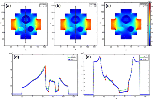
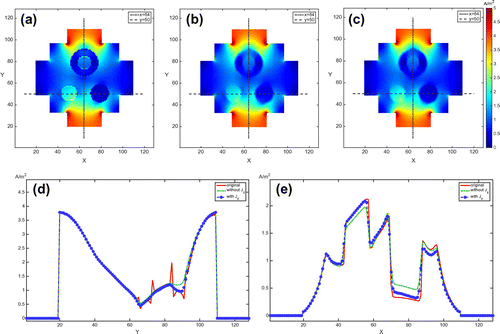
Figure 6. Images of the magnitudes of the current density distributions in the centre slice subject to the vertical injection current: low contrast case. (a) True current density. (b) Reconstructed current density without considering the influence of $J_z$ component. (c) Reconstruct current density using the two-step algorithm considering the influence of $J_z$ component. (d) and (e) are one-dimensional profiles along $x=64$ and $y=50$, respectively. Red, green and blue lines are from (a), (b) and (c), respectively.

We now have the following observation for the reconstructed current density.

Observation 3.6:

Let $\mathbf{J}$, ${\mathbf{J}}^0$, ${\mathbf{J}}_{xy}^{\ast }$, and ${\widehat{J}}_z$ be defined in Observation 3.1. Let ${\tilde{\mathbf{J}}}^0$ be given by (3.4(3.4) $$\begin{array}{c}\hfill \left\{\begin{array}{cc}{\mathrm{\nabla }}^2\tilde{\mathit{\psi }}=0\hfill & \text{in}\mathrm{\Omega },\hfill \\ \tilde{\mathit{\psi }}=\pm 1\hfill & \text{on}{\mathcal{E}}^{\pm },\hfill \\ \mathrm{\nabla }\tilde{\mathit{\psi }}·\mathbf{n}=0\hfill & \text{on}\mathit{\partial }\mathrm{\Omega }\backslash {\mathcal{E}}^{\pm }\hfill \end{array}\right.\end{array}$$(3.4) ) and (3.5(3.5) $$\begin{array}{c}\hfill {\tilde{\mathbf{J}}}^0:=\tilde{\mathit{\beta }}\mathrm{\nabla }\tilde{\mathit{\psi }},\end{array}$$(3.5) ), and ${\tilde{\mathbf{J}}}_{xy}^{\ast }$ be the least-squares solution of(3.6) $$\begin{array}{c}\hfill \left\{\begin{array}{cc}{\mathrm{\nabla }}_{xy}·{\tilde{\mathbf{J}}}_{xy}^{\ast }=-\frac{\mathit{\partial }}{\mathit{\partial }z}\left({\widehat{J}}_z-{\tilde{J}}_z^0\right)\hfill & \text{in}{\mathrm{\Omega }}_s,\hfill \\ {\mathrm{\nabla }}_{xy}^{\perp }·{\tilde{\mathbf{J}}}_{xy}^{\ast }=-\frac{1}{{\mathit{\mu }}_0}{\mathrm{\nabla }}^2{B}_z\hfill & \text{in}{\mathrm{\Omega }}_s,\hfill \\ {\tilde{\mathbf{J}}}_{xy}^{\ast }·\mathbf{n}=0\hfill & \text{on}\mathit{\partial }{\mathrm{\Omega }}_s.\hfill \end{array}\right.\end{array}$$(3.6)

Then, we have(3.7) $$\begin{array}{c}\hfill \begin{array}{cc}{∥{\mathbf{J}}_{xy}-\left({\tilde{\mathbf{J}}}_{xy}^0+{\tilde{\mathbf{J}}}_{xy}^{\ast }\right)∥}_{{\mathbf{L}}^2(\mathrm{\Omega })}^2\hfill & \le C\left(\underset{s}{max}{∥\frac{\mathit{\partial }}{\mathit{\partial }z}\left(J_z-{\widehat{J}}_z\right)∥}_{L^2({\mathrm{\Omega }}_s)}^2+{∥J_z-{\widehat{J}}_z∥}_{L^2(\mathrm{\Omega })}^2\right.\hfill \\ \hfill & +\left.{∥\mathbf{J}·\mathbf{n}-{\tilde{\mathbf{J}}}^0·\mathbf{n}∥}_{H^{-\frac{1}{2}}(\mathit{\partial }\mathrm{\Omega })}^2+\underset{s}{max}{∥\frac{\mathit{\partial }}{\mathit{\partial }z}\left({\tilde{J}}_z^0-J_z^0\right)∥}_{L^2({\mathrm{\Omega }}_s)}^2\right),\hfill \end{array}\end{array}$$(3.7)

where C is a positive constant.

Proof See Appendix A.2.

Remark 3.7:

The inequality (3.7(3.7) $$\begin{array}{c}\hfill \begin{array}{cc}{∥{\mathbf{J}}_{xy}-\left({\tilde{\mathbf{J}}}_{xy}^0+{\tilde{\mathbf{J}}}_{xy}^{\ast }\right)∥}_{{\mathbf{L}}^2(\mathrm{\Omega })}^2\hfill & \le C\left(\underset{s}{max}{∥\frac{\mathit{\partial }}{\mathit{\partial }z}\left(J_z-{\widehat{J}}_z\right)∥}_{L^2({\mathrm{\Omega }}_s)}^2+{∥J_z-{\widehat{J}}_z∥}_{L^2(\mathrm{\Omega })}^2\right.\hfill \\ \hfill & +\left.{∥\mathbf{J}·\mathbf{n}-{\tilde{\mathbf{J}}}^0·\mathbf{n}∥}_{H^{-\frac{1}{2}}(\mathit{\partial }\mathrm{\Omega })}^2+\underset{s}{max}{∥\frac{\mathit{\partial }}{\mathit{\partial }z}\left({\tilde{J}}_z^0-J_z^0\right)∥}_{L^2({\mathrm{\Omega }}_s)}^2\right),\hfill \end{array}\end{array}$$(3.7) ) says that if ${\widehat{J}}_z$ approximates $J_z$ well, then the approximation of ${\tilde{\mathbf{J}}}_{xy}^0+{\tilde{\mathbf{J}}}_{xy}^{\ast }$ to ${\mathbf{J}}_{xy}$ is determined by the differences between $\mathbf{J}·\mathbf{n}$ and ${\tilde{\mathbf{J}}}^0·\mathbf{n}$ on $\mathit{\partial }\mathrm{\Omega }$ and between $\frac{\mathit{\partial }}{\mathit{\partial }z}{\tilde{J}}_z^0$ and $\frac{\mathit{\partial }}{\mathit{\partial }z}{J}_z^0$ in ${\mathrm{\Omega }}_s$, which may give a better result compared with ${\mathbf{J}}_{xy}^{\text{rec}}$ in (2.2(2.2) $$\begin{array}{c}\hfill {\mathbf{J}}_{xy}\approx {\mathbf{J}}_{xy}^{\text{rec}}:=-\mathit{\beta }{\mathrm{\nabla }}_{xy}^{\perp }\mathrm{\Psi }-{\mathrm{\nabla }}_{xy}^{\perp }\mathit{\varphi }.\end{array}$$(2.2) ). The approximation error depends on the accuracy of the boundary condition of (3.4(3.4) $$\begin{array}{c}\hfill \left\{\begin{array}{cc}{\mathrm{\nabla }}^2\tilde{\mathit{\psi }}=0\hfill & \text{in}\mathrm{\Omega },\hfill \\ \tilde{\mathit{\psi }}=\pm 1\hfill & \text{on}{\mathcal{E}}^{\pm },\hfill \\ \mathrm{\nabla }\tilde{\mathit{\psi }}·\mathbf{n}=0\hfill & \text{on}\mathit{\partial }\mathrm{\Omega }\backslash {\mathcal{E}}^{\pm }\hfill \end{array}\right.\end{array}$$(3.4) ). It seems to be hard to generate the boundary current density which is close to that of the real case. But, one can design an experimental setting where the boundary current densities near the electrodes are similar to those of a presumed homogeneous domain. One possible method is the use of long recessed electrodes with a homogeneous conductive electrode gel. Similarly, we can handle $\frac{\mathit{\partial }}{\mathit{\partial }z}\left({\tilde{J}}_z^0-J_z^0\right)$.

Figure 7. Relative $L_2$ errors of the reconstructed current density images in the chosen slice near the centre of the imaging object: low contrast case. (a) and (b) are the plots for the horizontal and vertical current injections, respectively.

Figure 8. Conductivity images in the centre slice: high contrast case. (a) True conductivity distribution. (b) Reconstructed conductivity image without considering the influence of $J_z$ component. (c) Reconstructed conductivity image using the two-step algorithm considering the influence of $J_z$ component. (d) and (e) are one-dimensional profiles along $x=64$ and $y=50$, respectively. Red, green and blue lines are from (a), (b) and (c), respectively. Note that blue lines are much closer to red lines.

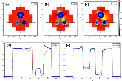
Figure 9. Relative $L_2$ error plots in three regions of interest (ROI): high contrast case. (a) shows the selected ROIs. (b), (c) and (d) are the relative $L_2$ error plots for the red, blue and green ROIs, respectively.

Figure 10. Images of the magnitudes of the current density distributions in the centre slice subject to the horizontal injection current: high contrast case. (a) True current density. (b) Reconstructed current density without considering the influence of $J_z$ component. (c) Reconstruct current density using the two-step algorithm considering the influence of $J_z$ component. (d) and (e) are one-dimensional profiles along $x=64$ and $y=50$, respectively. Red, green and blue lines are from (a), (b) and (c), respectively.

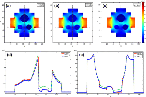
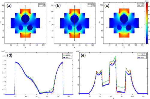
Figure 11. Images of the magnitudes of the current density distributions in the centre slice subject to the vertical injection current: high contrast case. (a) True current density. (b) Reconstructed current density without considering the influence of $J_z$ component. (c) Reconstruct current density using the two-step algorithm considering the influence of $J_z$ component. (d) and (e) are one-dimensional profiles along $x=64$ and $y=50$, respectively. Red, green and blue lines are from (a), (b) and (c), respectively.

To reconstruct a conductivity image, the following Poisson equation is derived on the imaging slice ${\mathrm{\Omega }}_s$. Taking the two-dimensional divergence to (1.4(1.4) $$\begin{array}{c}\hfill {\mathrm{\nabla }}_{xy}ln\mathit{\sigma }=\frac{1}{{\mathit{\mu }}_0}{\mathbf{A}}^{-1}\left(\begin{array}{c}{\mathrm{\nabla }}^2{B}_{z,1}\\ {\mathrm{\nabla }}^2{B}_{z,2}\end{array}\right),\end{array}$$(1.4) ),(3.8) $$\begin{array}{c}\hfill \left\{\begin{array}{cc}{\mathrm{\nabla }}_{xy}^{2}ln\mathit{\sigma }={\mathrm{\nabla }}_{xy}·\left(\frac{1}{{\mathit{\mu }}_0}{\tilde{\mathbf{A}}}^{-1}\left(\begin{array}{c}{\mathrm{\nabla }}^2{B}_{z,1}\\ {\mathrm{\nabla }}^2{B}_{z,2}\end{array}\right)\right)\hfill & \text{in}{\mathrm{\Omega }}_s,\hfill \\ ln\mathit{\sigma }=ln{\mathit{\sigma }}_s\hfill & \text{in}\mathit{\partial }{\mathrm{\Omega }}_s,\hfill \end{array}\right.\end{array}$$(3.8)

where(3.9) $$\begin{array}{c}\hfill \tilde{\mathbf{A}}:=\left(\begin{array}{cc}-{\tilde{J}}_{y,1}& {\tilde{J}}_{x,1}\\ -{\tilde{J}}_{y,2}& {\tilde{J}}_{x,2}\end{array}\right),{\tilde{\mathbf{J}}}_{xy,i}:={\tilde{\mathbf{J}}}_{xy,i}^0+{\tilde{\mathbf{J}}}_{xy,i}^{\ast }\text{for}i=1,2.\end{array}$$(3.9)

Now, the remaining problem is how to get ${\widehat{J}}_z$ which is close to $J_z$. It is a most important issue for the approximated current density reconstruction as shown in Observation 3.6. In this paper, we will reduce the scope of the study only to the process to include the influence of $J_z$ for the absolute conductivity reconstruction. To obtain ${\widehat{J}}_z$, (1.1(1.1) $$\begin{array}{c}\hfill \left\{\begin{array}{c}\mathrm{\nabla }·\mathit{\sigma }\mathrm{\nabla }u=0\text{in}\mathrm{\Omega },\hfill \\ I={\int }_{{\mathcal{E}}^{+}}\mathit{\sigma }\mathrm{\nabla }u·\mathbf{n}\mathrm{d}s,=-{\int }_{{\mathcal{E}}^{-}}\mathit{\sigma }\mathrm{\nabla }u·\mathbf{n}\mathrm{d}s,\hfill \\ {\mathit{\sigma }\mathrm{\nabla }u\times \mathbf{n}|}_{{\mathcal{E}}^{+}\cup {\mathcal{E}}^{-}}=0,\hfill \\ \mathit{\sigma }\mathrm{\nabla }u·\mathbf{n}=0\text{on}\mathit{\partial }\mathrm{\Omega }\backslash \overline{{\mathcal{E}}^{+}\cup {\mathcal{E}}^{-}},\hfill \end{array}\right.\end{array}$$(1.1) ) is solved with the conductivity $\mathit{\sigma }$ obtained from (3.8(3.8) $$\begin{array}{c}\hfill \left\{\begin{array}{cc}{\mathrm{\nabla }}_{xy}^{2}ln\mathit{\sigma }={\mathrm{\nabla }}_{xy}·\left(\frac{1}{{\mathit{\mu }}_0}{\tilde{\mathbf{A}}}^{-1}\left(\begin{array}{c}{\mathrm{\nabla }}^2{B}_{z,1}\\ {\mathrm{\nabla }}^2{B}_{z,2}\end{array}\right)\right)\hfill & \text{in}{\mathrm{\Omega }}_s,\hfill \\ ln\mathit{\sigma }=ln{\mathit{\sigma }}_s\hfill & \text{in}\mathit{\partial }{\mathrm{\Omega }}_s,\hfill \end{array}\right.\end{array}$$(3.8) ) with ${\tilde{\mathbf{J}}}_{xy}^0$ only. Then, ${\widehat{J}}_z$ does not satisfy (3.2(3.2) $$\begin{array}{c}\hfill {\int }_{{\mathrm{\Omega }}_s}\frac{\mathit{\partial }}{\mathit{\partial }z}\left({\widehat{J}}_z-J_z^0\right)\mathrm{d}x\mathrm{d}y=0\end{array}$$(3.2) ) anymore. Hence, we find a least-squares solution of (3.3(3.3) $$\begin{array}{c}\hfill \left\{\begin{array}{cc}{\mathrm{\nabla }}_{xy}·{\mathbf{J}}_{xy}^{\ast }=-\frac{\mathit{\partial }}{\mathit{\partial }z}\left({\widehat{J}}_z-J_z^0\right)\hfill & \text{in}{\mathrm{\Omega }}_s,\hfill \\ {\mathrm{\nabla }}_{xy}^{\perp }·{\mathbf{J}}_{xy}^{\ast }=-\frac{1}{{\mathit{\mu }}_0}{\mathrm{\nabla }}^2{B}_z\hfill & \text{in}{\mathrm{\Omega }}_s,\hfill \\ {\mathbf{J}}_{xy}^{\ast }·\mathbf{n}=0\hfill & \text{on}\mathit{\partial }{\mathrm{\Omega }}_s.\hfill \end{array}\right.\end{array}$$(3.3) ). It is easy to check that Observation 3.1 holds for such ${\widehat{J}}_z$. Combining all together, the two-step $B_z$ algorithm is summarized below.

$\left[\mathbf{Step}\mathbf{1}\mathbf{to}\mathbf{acquire}\mathbf{a}\mathbf{prior}\mathbf{information}{\widehat{\mathbf{J}}}_{\mathbf{z}}\right]$

(i)	For two injection currents $I_j$ and corresponding magnetic flux densities $B_{z,j}$ for $j=1,2$, solve (3.4(3.4) $$\begin{array}{c}\hfill \left\{\begin{array}{cc}{\mathrm{\nabla }}^2\tilde{\mathit{\psi }}=0\hfill & \text{in}\mathrm{\Omega },\hfill \\ \tilde{\mathit{\psi }}=\pm 1\hfill & \text{on}{\mathcal{E}}^{\pm },\hfill \\ \mathrm{\nabla }\tilde{\mathit{\psi }}·\mathbf{n}=0\hfill & \text{on}\mathit{\partial }\mathrm{\Omega }\backslash {\mathcal{E}}^{\pm }\hfill \end{array}\right.\end{array}$$(3.4) ) to get ${\tilde{\mathbf{J}}}_{xy,j}^0$ by (3.5(3.5) $$\begin{array}{c}\hfill {\tilde{\mathbf{J}}}^0:=\tilde{\mathit{\beta }}\mathrm{\nabla }\tilde{\mathit{\psi }},\end{array}$$(3.5) ).
(ii)	Solve$$\begin{array}{c}\hfill \left\{\begin{array}{cc}{\mathrm{\nabla }}_{xy}·{\mathbf{Y}}_j=0\hfill & \text{in}{\mathrm{\Omega }}_s,\hfill \\ {\mathrm{\nabla }}_{xy}^{\perp }·{\mathbf{Y}}_j=-\frac{1}{{\mathit{\mu }}_0}{\mathrm{\nabla }}^2{B}_{z,j}\hfill & \text{in}{\mathrm{\Omega }}_s,\hfill \\ {\mathbf{Y}}_j·\mathbf{n}=0\hfill & \text{on}\mathit{\partial }{\mathrm{\Omega }}_s\hfill \end{array}\right.\end{array}$$ for $j=1,2$.
(iii)	Set ${\tilde{\mathbf{J}}}_{xy,j}:={\tilde{\mathbf{J}}}_{xy,j}^0+{\mathbf{Y}}_j$ for $j=1,2$ and compute the conductivity $\mathit{\sigma }$ by solving (3.8(3.8) $$\begin{array}{c}\hfill \left\{\begin{array}{cc}{\mathrm{\nabla }}_{xy}^{2}ln\mathit{\sigma }={\mathrm{\nabla }}_{xy}·\left(\frac{1}{{\mathit{\mu }}_0}{\tilde{\mathbf{A}}}^{-1}\left(\begin{array}{c}{\mathrm{\nabla }}^2{B}_{z,1}\\ {\mathrm{\nabla }}^2{B}_{z,2}\end{array}\right)\right)\hfill & \text{in}{\mathrm{\Omega }}_s,\hfill \\ ln\mathit{\sigma }=ln{\mathit{\sigma }}_s\hfill & \text{in}\mathit{\partial }{\mathrm{\Omega }}_s,\hfill \end{array}\right.\end{array}$$(3.8) ) for all imaging slices ${\mathrm{\Omega }}_s$.
(iv)	Get ${\widehat{J}}_{z,j}$ by solving (1.1(1.1) $$\begin{array}{c}\hfill \left\{\begin{array}{c}\mathrm{\nabla }·\mathit{\sigma }\mathrm{\nabla }u=0\text{in}\mathrm{\Omega },\hfill \\ I={\int }_{{\mathcal{E}}^{+}}\mathit{\sigma }\mathrm{\nabla }u·\mathbf{n}\mathrm{d}s,=-{\int }_{{\mathcal{E}}^{-}}\mathit{\sigma }\mathrm{\nabla }u·\mathbf{n}\mathrm{d}s,\hfill \\ {\mathit{\sigma }\mathrm{\nabla }u\times \mathbf{n}|}_{{\mathcal{E}}^{+}\cup {\mathcal{E}}^{-}}=0,\hfill \\ \mathit{\sigma }\mathrm{\nabla }u·\mathbf{n}=0\text{on}\mathit{\partial }\mathrm{\Omega }\backslash \overline{{\mathcal{E}}^{+}\cup {\mathcal{E}}^{-}},\hfill \end{array}\right.\end{array}$$(1.1) ) with $\mathit{\sigma }$ obtained from step (iii).

$\left[\mathbf{Step}\mathbf{2}\mathbf{to}\mathbf{reconstruct}\mathbf{current}\mathbf{density}\mathbf{and}\mathbf{conductivity}\right]$

(I)

Apply (3.6(3.6) $$\begin{array}{c}\hfill \left\{\begin{array}{cc}{\mathrm{\nabla }}_{xy}·{\tilde{\mathbf{J}}}_{xy}^{\ast }=-\frac{\mathit{\partial }}{\mathit{\partial }z}\left({\widehat{J}}_z-{\tilde{J}}_z^0\right)\hfill & \text{in}{\mathrm{\Omega }}_s,\hfill \\ {\mathrm{\nabla }}_{xy}^{\perp }·{\tilde{\mathbf{J}}}_{xy}^{\ast }=-\frac{1}{{\mathit{\mu }}_0}{\mathrm{\nabla }}^2{B}_z\hfill & \text{in}{\mathrm{\Omega }}_s,\hfill \\ {\tilde{\mathbf{J}}}_{xy}^{\ast }·\mathbf{n}=0\hfill & \text{on}\mathit{\partial }{\mathrm{\Omega }}_s.\hfill \end{array}\right.\end{array}$$(3.6) ) to obtain ${\tilde{\mathbf{J}}}_{xy,j}^{\ast }$ using computed ${\tilde{J}}_{z,j}^0$ and ${\widehat{J}}_{z,j}$ in steps i and iv, respectively, for $j=1,2$.

(II)

Reconstruct the conductivity $\mathit{\sigma }$ by solving (3.8(3.8) $$\begin{array}{c}\hfill \left\{\begin{array}{cc}{\mathrm{\nabla }}_{xy}^{2}ln\mathit{\sigma }={\mathrm{\nabla }}_{xy}·\left(\frac{1}{{\mathit{\mu }}_0}{\tilde{\mathbf{A}}}^{-1}\left(\begin{array}{c}{\mathrm{\nabla }}^2{B}_{z,1}\\ {\mathrm{\nabla }}^2{B}_{z,2}\end{array}\right)\right)\hfill & \text{in}{\mathrm{\Omega }}_s,\hfill \\ ln\mathit{\sigma }=ln{\mathit{\sigma }}_s\hfill & \text{in}\mathit{\partial }{\mathrm{\Omega }}_s,\hfill \end{array}\right.\end{array}$$(3.8) ) with ${\tilde{\mathbf{J}}}_{xy,j}:={\tilde{\mathbf{J}}}_{xy,j}^0+{\tilde{\mathbf{J}}}_{xy,j}^{\ast }$ for $j=1,2$.

The uniqueness of the reconstructed conductivity image remains as an open problem in the three-dimensional case [18]. More precisely, if $|det(\tilde{\mathbf{A}})|>0$ in $\mathrm{\Omega }$, the unique reconstruction of the conductivity is guaranteed, where $\tilde{\mathbf{A}}$ is in (3.9(3.9) $$\begin{array}{c}\hfill \tilde{\mathbf{A}}:=\left(\begin{array}{cc}-{\tilde{J}}_{y,1}& {\tilde{J}}_{x,1}\\ -{\tilde{J}}_{y,2}& {\tilde{J}}_{x,2}\end{array}\right),{\tilde{\mathbf{J}}}_{xy,i}:={\tilde{\mathbf{J}}}_{xy,i}^0+{\tilde{\mathbf{J}}}_{xy,i}^{\ast }\text{for}i=1,2.\end{array}$$(3.9) ).

Figure 12. Relative $L_2$ errors of the reconstructed current density images in the chosen slice near the centre of the imaging object: high contrast case. (a) and (b) are the plots for the horizontal and vertical current injections, respectively.

Figure 13. Conductivity images in the centre slice: low contrast case with added noise. (a) True conductivity distribution. (b) Reconstructed conductivity image without considering the influence of $J_z$ component. (c) Reconstructed conductivity image using the two-step algorithm considering the influence of $J_z$ component. (d) and (e) are one-dimensional profiles along $x=64$ and $y=50$, respectively.

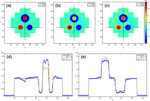
Figure 14. Relative $L_2$ error plots in three regions of interest (ROI): low contrast case with added noise. (a) shows the selected ROIs. (b), (c) and (d) are the relative $L_2$ error plots for the red, blue and green ROIs, respectively.

Figure 15. Conductivity images in the centre slice: high contrast case with added noise. (a) True conductivity distribution. (b) Reconstructed conductivity image without considering the influence of $J_z$ component. (c) Reconstructed conductivity image using the two-step algorithm considering the influence of $J_z$ component. (d) and (e) are one-dimensional profiles along $x=64$ and $y=50$, respectively.

4. Numerical simulations and phantom experiments

4.1. Numerical simulations

We conducted numerical simulations to verify the proposed algorithm. We set the domain $\mathrm{\Omega }$ as a cube of size $100\times 100\times 100{\mathrm{mm}}^3$ with two pairs of electrodes of size $50\times 50\times 20{\mathrm{mm}}^3$ as in Figure 2(a). The amplitude of the injected current was 10 mA per electrodes pair. We placed three objects with different conductivity values as shown in Figure 2(b). Each object was an ellipsoid with different size and location; see Table 1 for more details. To make an unstructured tetrahedral mesh for the numerical simulation, we used the TetGen [30]. The total number of vertices and tetrahedrons were 732,353 and 4,532,306, respectively. The minimum and maximum radius of circumscribed spheres are 0.49 and $1.5\mathrm{mm}$, respectively. The size of the imaging domain was $128\times 128$ pixels for each $s=1,\dots ,128$. According to the field of view ($200\times 200\times 200{\mathrm{mm}}^3$) and number of voxel grid ($128\times 128\times 128$), the voxel length is $1.56\mathrm{mm}$. Therefore, the computational mesh size is small enough to resolve the imaging voxel grid. To solve (3.4(3.4) $$\begin{array}{c}\hfill \left\{\begin{array}{cc}{\mathrm{\nabla }}^2\tilde{\mathit{\psi }}=0\hfill & \text{in}\mathrm{\Omega },\hfill \\ \tilde{\mathit{\psi }}=\pm 1\hfill & \text{on}{\mathcal{E}}^{\pm },\hfill \\ \mathrm{\nabla }\tilde{\mathit{\psi }}·\mathbf{n}=0\hfill & \text{on}\mathit{\partial }\mathrm{\Omega }\backslash {\mathcal{E}}^{\pm }\hfill \end{array}\right.\end{array}$$(3.4) ), we applied the ${\mathcal{P}}_1$ finite-element method for the discretization. Since the standard ${\mathcal{P}}_1$ element was used, the degree of freedom is almost same as the total number of nodes. We used the least-squares finite-element method [31] with the ${\mathcal{P}}_1$ element for solving (3.6(3.6) $$\begin{array}{c}\hfill \left\{\begin{array}{cc}{\mathrm{\nabla }}_{xy}·{\tilde{\mathbf{J}}}_{xy}^{\ast }=-\frac{\mathit{\partial }}{\mathit{\partial }z}\left({\widehat{J}}_z-{\tilde{J}}_z^0\right)\hfill & \text{in}{\mathrm{\Omega }}_s,\hfill \\ {\mathrm{\nabla }}_{xy}^{\perp }·{\tilde{\mathbf{J}}}_{xy}^{\ast }=-\frac{1}{{\mathit{\mu }}_0}{\mathrm{\nabla }}^2{B}_z\hfill & \text{in}{\mathrm{\Omega }}_s,\hfill \\ {\tilde{\mathbf{J}}}_{xy}^{\ast }·\mathbf{n}=0\hfill & \text{on}\mathit{\partial }{\mathrm{\Omega }}_s.\hfill \end{array}\right.\end{array}$$(3.6) ). To obtain the conductivity, we solved (3.8(3.8) $$\begin{array}{c}\hfill \left\{\begin{array}{cc}{\mathrm{\nabla }}_{xy}^{2}ln\mathit{\sigma }={\mathrm{\nabla }}_{xy}·\left(\frac{1}{{\mathit{\mu }}_0}{\tilde{\mathbf{A}}}^{-1}\left(\begin{array}{c}{\mathrm{\nabla }}^2{B}_{z,1}\\ {\mathrm{\nabla }}^2{B}_{z,2}\end{array}\right)\right)\hfill & \text{in}{\mathrm{\Omega }}_s,\hfill \\ ln\mathit{\sigma }=ln{\mathit{\sigma }}_s\hfill & \text{in}\mathit{\partial }{\mathrm{\Omega }}_s,\hfill \end{array}\right.\end{array}$$(3.8) ) using the ${\mathcal{P}}_1$ finite-element method as well. Note that, by the finite-element methods, we do not take the divergence operator to the right-hand side of (3.8(3.8) $$\begin{array}{c}\hfill \left\{\begin{array}{cc}{\mathrm{\nabla }}_{xy}^{2}ln\mathit{\sigma }={\mathrm{\nabla }}_{xy}·\left(\frac{1}{{\mathit{\mu }}_0}{\tilde{\mathbf{A}}}^{-1}\left(\begin{array}{c}{\mathrm{\nabla }}^2{B}_{z,1}\\ {\mathrm{\nabla }}^2{B}_{z,2}\end{array}\right)\right)\hfill & \text{in}{\mathrm{\Omega }}_s,\hfill \\ ln\mathit{\sigma }=ln{\mathit{\sigma }}_s\hfill & \text{in}\mathit{\partial }{\mathrm{\Omega }}_s,\hfill \end{array}\right.\end{array}$$(3.8) ) because we formulate a weak form using the integration by parts. The conjugate gradient method was applied for matrix inversions in both cases. We used a PC with a 3.4 GHz Intel CPU, 32 GB memory and Ubuntu 14.04 LTS operating system (Canonical Ltd., UK).

Table 1. Description of the conductivity distribution. The unit for lengths is mm.

$r_1^2\le \frac{{(x-x_0)}^2}{a^2}+\frac{{(x-y_0)}^2}{b^2}+\frac{{(x-z_0)}^2}{c^2}\le r_2^2$
Object	$x_0$	$y_0$	$z_0$	a	b	c	$r_1$	$r_2$	Value
1	22	-22	10	16	16	20	0	1	0.02081 S/m
2	-22	-22	-10	13	13	20	0	1	0.26671 S/m
3	0	22	0	20	20	40	0	0.5	0.26671 S/m
4	0	22	0	20	20	40	0.5	1	0.02081 S/m

Figure 16. Relative $L_2$ error plots in three regions of interest (ROI): high contrast case with added noise. (a) shows the selected ROIs. (b), (c) and (d) are the relative $L_2$ error plots for the red, blue and green ROIs, respectively.

Figure 17. Experiment setup. (a) Cylindrical phantom inside the RF coil. (b) Diagram of the conductivity distribution. (c) MR magnitude image at the centre of the phantom.

Figure 18. Results of phantom experiment. Images in the top row are the MR magnitude images in three different slices. The middle row shows the reconstructed conductivity images without considering the influence of $J_z$ component. The bottom row shows the reconstructed conductivity images using the two-step algorithm considering the influence of $J_z$ component.

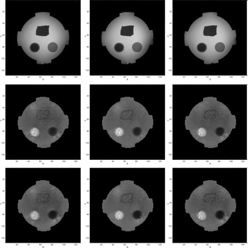
Figure 19. Magnified images of the agar regions of the phantom. The top row provides MR images with region of interest. The middle row shows the reconstructed conductivity images without considering the influence of $J_z$ component. The bottom row shows the reconstructed conductivity images using the two-step algorithm considering the influence of $J_z$ component.

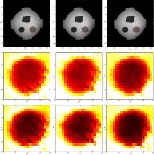
Figure 20. Means (dots) and standard deviations (bars) of the reconstructed conductivity values in 10 local regions. Red lines are from the reconstructed conductivity images without considering the influence of $J_z$ component, and the blue lines are from the reconstructed conductivity images using the two-step algorithm considering the influence of $J_z$ component. Inside (a) TX-151 object (low contrast), (b) muscle tissue (low contrast), and (c) agar object (high contrast).

4.1.1. Low contrast case

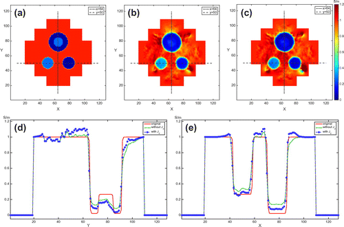
We set the background conductivity as 0.13 S/m and let the maximum contrast does not exceed 10 times. Figure 3(a) shows the true conductivity distribution in the centre slice. Figure 3(b) and (c) show the reconstructed results without and with considering the influence of $J_z$ component, respectively. One can consider the proposed algorithm without considering the influence of $J_z$ component as the non-iterative harmonic $B_z$ algorithm [26]. According to the initial conductivity configuration, the objects 2 and 3 should have similar colour values in the image. In (b), however, two objects appeared to have different conductivity values; the difference is 0.0968. The result in (c) using the proposed two-step $B_z$ algorithm recovered conductivity values with a difference 0.0382. Figure 3(d) and (e) are one-dimensional profiles along the vertical line of $x=64$ and the horizontal line of $y=50$, respectively. In Figure 4, we provided the relative $L_2$ errors of the reconstructed conductivity values in a few regions of interest on the selected slices near the centre of the imaging object. We can identify the theoretical observation of the influence of $J_z$ component in the numerical simulation result.

In addition, to show the performance of the proposed method, we used the reconstructed current density images. Figures 5 and 6 are reconstructed images of the magnitudes of the internal current density distributions subject to the current injections along the horizontal and vertical directions, respectively. As shown in the figures, the global behaviour of the current flow are similar in both cases with and without $J_z$ component correction. However, the details of the current density near the region of conductivity changing are different so that these produce more accurate conductivity; the proposed method can provide an effective method to compute the current density near the region of conductivity contrast changing. We provided the relative $L_2$ errors of the reconstructed current density distributions for several slices in Figure 7.

4.1.2. High contrast case

We tested the algorithm using a different model with high conductivity contrast. The background conductivity was 1.0 S/m and the maximum contrast was almost 50 times. Figure 8(a) shows the true conductivity distribution. Figure 8(b) and (c) show the reconstructed results without and with considering the influence of $J_z$ component, respectively. The results clearly show that the proposed two-step $B_z$ algorithm is much superior to the single-step method; the conductivity differences between objects 2 and 3 are 0.1189 and 0.0074 in (b) and (c), respectively. The relative $L_2$ errors in the selected regions of interest also support our observation; see Figure 9. We could obtain similar results in the reconstructed current density images. The errors of the reconstructed current density image without considering the influence of $J_z$ component are 0.1404 and 0.153 whereas the two-step algorithm produced the current density image with errors 0.102 and 0.125 for horizontal and vertical injections, respectively. See Figures 10 and 11 for the cases of the horizontal and vertical current injections, respectively. The relative $L_2$ errors of a few selected slices near the centre of the imaging object are plotted in Figure 12. As show in Figure 8, we cannot obtain the conductivity contrast changing when applying the first step of the proposed algorithm, since $B_z$ is generated by the two-dimensional current density distribution. In the second step of the proposed algorithm, we take an advantage of ${\widehat{J}}_z$ from the first step, which provides the geometrical change of the current density given by the conductivity distribution along the z-direction. The proposed method provides the information of two-dimensional reconstructed current contributed on the xy-plane by $B_z$ with the geometrical change of the current density along the z-direction. Therefore, the proposed algorithm handles properly the high contrast conductivity case that is not well treated by the conventional MREIT algorithms.

4.1.3. Added noise case

To check the robustness of the proposed algorithm, we added zero-mean Gaussian random noise N to the simulated $B_z$ data so that the signal-to-noise ratio (SNR) was 50 dB in both low and high contrast cases. The SNR of the simulated $B_z$ is defined by $10{log}_{10}\left(\frac{\text{Var}(B_z+N)}{\text{Var}(N)}\right)$, where $\text{Var}(·)$ is the variance. To ensure the smoothness of ${\mathrm{\nabla }}^2{B}_z$, we applied the isotropic diffusion of a small time duration, for example 0.3 s. Figures 13, 14 and 15, 16 illustrate the reconstructed conductivity images for the low and high contrast cases, respectively. We can see that performance of the proposed two-step $B_z$ algorithm is better than that of the single-step method in the cases with the added noise as well.

4.2. Phantom experiments

We performed phantom experiments to verify the applicability of the proposed two-step $B_z$ algorithm. We prepared a cylindrical acrylic phantom with two pairs of electrodes. The inner and outer diameters of the acrylic phantom were 160 and 180 mm, respectively. Its height was 120 mm. We placed three anomalies inside the phantom, having different conductivity values: agar with 0.1 S/m, TX-151 with 1.5 S/m and muscle tissue with 0.6 S/m. The background of the phantom was filled with a saline of 1.0 S/m. For more details, see Figure 17(a) and (b). We injected 30 mA current for 29 ms using a custom-designed MREIT current source [32] synchronized with the injection current non-linear encoding multi-spin-echo pulse sequence [33] between each pair of electrodes. The imaging parameters are provided in Table 2. Figure 17(c) is the MR magnitude image at the centre of the phantom.

Table 2. MREIT experiment parameters.

MR system	Philips Acheiva 3.0T
RF coil	Head Coil (1 channel Tx/Rx)
Repetition time (TR)	1200 ms
Echo time (TE)	30 ms
Number of excitation (NEX)	24
Imaging time	61 min
Field of view	$260\times 260{\mathrm{mm}}^2$
Slice thickness	4 mm
Imaging matrix	$128\times 128$ pixels

In Figure 18, the images in the top row are MR magnitude images of three different imaging slices. The reconstructed conductivity images without considering the influence of $J_z$ component are shown in the middle row. In the bottom row, we plotted the reconstructed conductivity images using the two-step algorithm considering the influence of $J_z$ component. Since the conductivity values of the TX-151 object and muscle tissue were similar to that of the background, the influence of $J_z$ component appears to be small. However, we can see that the two-step algorithm recovered accurate conductivity values of the agar object with a relatively high contrast. We illustrated the magnified images of the agar region in Figure 19.

Comparing with the numerical simulation results, local fluctuations of the reconstructed conductivity images were high. Instead of plotting one-dimensional profiles of the reconstructed conductivity images, we provided statistical information of the reconstructed conductivity values of the local regions inside the phantom in Figure 20. We selected circular-shaped local regions with radius of 5 pixels in the agar, TX-151, and muscle regions. We computed the means and standard deviations of the reconstructed conductivity values from 10 local regions in the middle imaging slices. As stated above, we can see that the two-step algorithm is especially advantageous in the region with a high conductivity contrast.

5. Conclusion and remark

We proposed the non-iterative two-step $B_z$ algorithm for conductivity and current density image reconstructions to improve the image quality. The improved performance stemmed from the two-step approach of incorporating the influence of the non-transversal component of the current density. Numerical simulation results showed that the proposed algorithm can successfully reconstruct high-quality conductivity and current density images. The proposed algorithm is especially advantageous for the case of high conductivity contrast. We expect that this advantage will be more useful in experimental studies of animal and human subjects.

One disadvantage of the proposed method is the large amount of computation time to numerically solve the three-dimensional elliptic problems. More precisely, the proposed method requires twice the computational cost comparing with [27,28]. For reducing the computational time, we may adopt some acceleration techniques for matrix inversion. In this study, we used ViennaCL [34] to implement the conjugate gradient method using graphic processor units (GPU). The parallel conjugate gradient algorithm was operated by a GPU (NVIDIA GTX TitanX, Nvidia, USA). The overall computation time was 10 min. The computations needed to implement the proposed algorithm can be parallelized naturally because they are two-dimensional problems in each slice. Therefore, the required computing time can be reduced by utilizing parallel computing tools, for example, message passing interface and OpenMP as well as computer unified device architecture. 1Friedrichs’ inequality [35]: Suppose that ${\mathrm{\Omega }}_s$ is a simply connected bounded Lipschitz domain in ${\mathbf{R}}^2$. Then every function $\mathbf{u}$ of ${\left[H_1({\mathrm{\Omega }}_s)\right]}^2$ with $\mathbf{u}·\mathbf{n}=0$ on $\mathit{\partial }{\mathrm{\Omega }}_s$ satisfies that ${\Vert \mathbf{u}\Vert }_{{\mathbf{L}}^2({\mathrm{\Omega }}_s)}\le C\left(\Vert {\mathrm{\nabla }}_{xy}{·\mathbf{u}\Vert }_{L^2({\mathrm{\Omega }}_s)}+{\Vert {\mathrm{\nabla }}_{xy}^{\perp }·\mathbf{u}\Vert }_{L^2({\mathrm{\Omega }}_s)}\right)$ where the constant $C>0$ depends only on ${\mathrm{\Omega }}_s$.

Additional information

Funding

Kiwan Jeon was supported by the National Institute for Mathematical Sciences (NIMS) grant funded by the Korean government [number A21300000]. Chang-Ock Lee was supported by the NRF grant funded by MSIP (NRF-2014R1A2A2A01006497). Eung Je Woo was supported by the NRF grant (NRF-2014R1A2A1A09006320).

Notes

No potential conflict of interest was reported by the authors.

2 Friedrichs’ inequality [35]: Suppose that ${\mathrm{\Omega }}_s$ is a simply connected bounded Lipschitz domain in ${\mathbf{R}}^2$. Then every function $\mathbf{u}$ of ${\left[H_1({\mathrm{\Omega }}_s)\right]}^2$ with $\mathbf{u}·\mathbf{n}=0$ on $\mathit{\partial }{\mathrm{\Omega }}_s$ satisfies that ${\Vert \mathbf{u}\Vert }_{{\mathbf{L}}^2({\mathrm{\Omega }}_s)}\le C\left(\Vert {\mathrm{\nabla }}_{xy}{·\mathbf{u}\Vert }_{L^2({\mathrm{\Omega }}_s)}+{\Vert {\mathrm{\nabla }}_{xy}^{\perp }·\mathbf{u}\Vert }_{L^2({\mathrm{\Omega }}_s)}\right)$ where the constant $C>0$ depends only on ${\mathrm{\Omega }}_s$.

Appendix 1

The Proof of Observation 3.1

Proof Let$$\begin{array}{c}\hfill W:={\mathbf{J}}_{xy}-\left({\mathbf{J}}_{xy}^0+{\mathbf{J}}_{xy}^{\ast }\right).\end{array}$$

From Ampère’s law, W satisfies the following system:$$\begin{array}{c}\hfill \left\{\begin{array}{cc}{\mathrm{\nabla }}_{xy}·W=-\frac{\mathit{\partial }}{\mathit{\partial }z}\left(J_z-{\widehat{J}}_z\right)\hfill & \text{in}{\mathrm{\Omega }}_s,\hfill \\ {\mathrm{\nabla }}_{xy}^{\perp }·W=0\hfill & \text{in}{\mathrm{\Omega }}_s,\hfill \\ W·\mathbf{n}=0\hfill & \text{on}\mathit{\partial }{\mathrm{\Omega }}_s.\hfill \end{array}\right.\end{array}$$

From the Friedrichs inequality², we have$$\begin{array}{cc}\hfill {∥W∥}_{{\mathbf{L}}^2({\mathrm{\Omega }}_s)}& \le C\left({∥{\mathrm{\nabla }}_{xy}·W∥}_{L^2({\mathrm{\Omega }}_s)}+{∥{\mathrm{\nabla }}_{xy}^{\perp }W∥}_{L^2({\mathrm{\Omega }}_s)}\right)\hfill \\ \hfill & =C{∥\frac{\mathit{\partial }}{\mathit{\partial }z}\left(J_z-{\widehat{J}}_z\right)∥}_{L^2({\mathrm{\Omega }}_s)}.\hfill \end{array}$$

The Proof of Observation 3.6

Proof Clearly, we have$$\begin{array}{cc}\hfill {∥{\mathbf{J}}_{xy}-\left({\tilde{\mathbf{J}}}_{xy}^0+{\tilde{\mathbf{J}}}_{xy}^{\ast }\right)∥}_{{\mathbf{L}}^2(\mathrm{\Omega })}^2& \le {∥\mathbf{J}-\left({\tilde{\mathbf{J}}}^0+\left(\begin{array}{c}{\tilde{J}}_x^{\ast }\\ {\tilde{J}}_y^{\ast }\\ {\widehat{J}}_z-{\tilde{J}}_z^0\end{array}\right)\right)∥}_{{\mathbf{L}}^2(\mathrm{\Omega })}^2\hfill \\ \hfill & ={∥\mathbf{J}-\left({\mathbf{J}}^0+\left(\begin{array}{c}{J}_x^{\ast }\\ J_y^{\ast }\\ {\widehat{J}}_z-J_z^0\end{array}\right)\right)+\left(\begin{array}{c}{J}_x^0-{\tilde{J}}_x^0\\ J_y^0-{\tilde{J}}_y^0\\ 0\end{array}\right)+\left(\begin{array}{c}{J}_x^{\ast }-{\tilde{J}}_x^{\ast }\\ J_y^{\ast }-{\tilde{J}}_y^{\ast }\\ 0\end{array}\right)∥}_{{\mathbf{L}}^2(\mathrm{\Omega })}^2\hfill \\ \hfill & \le 3(\Vert \mathbf{J}-({\mathbf{J}}^0+\left(\begin{array}{c}{J}_x^{\ast }\\ J_y^{\ast }\\ {\widehat{J}}_z-J_z^0\end{array}\right)){\Vert }_{{\mathbf{L}}^2(\mathrm{\Omega })}^2\hfill \\ \hfill & +\Vert {\mathbf{J}}^0-{\tilde{\mathbf{J}}}^0{\Vert }_{{\mathbf{L}}^2(\mathrm{\Omega })}^2+\Vert {\mathbf{J}}_{xy}^{\ast }-{\tilde{\mathbf{J}}}_{xy}^{\ast }{\Vert }_{{\mathbf{L}}^2(\mathrm{\Omega })}^2).\hfill \end{array}$$

The first term in the right-hand side of the above inequality can be estimated as follows; from Observation 3.1,$$\begin{array}{cc}\hfill {∥\mathbf{J}-\left({\mathbf{J}}^0+\left(\begin{array}{c}{J}_x^{\ast }\\ J_y^{\ast }\\ {\widehat{J}}_z-J_z^0\end{array}\right)\right)∥}_{{\mathbf{L}}^2(\mathrm{\Omega })}^2& \le \int \left[{\int }_{{\mathrm{\Omega }}_s}{\left|{\mathbf{J}}_{xy}-\left({\mathbf{J}}_{xy}^0+{\mathbf{J}}_{xy}^{\ast }\right)\right|}^2\mathrm{d}x\mathrm{d}y\right]\mathrm{d}z+{\int }_{\mathrm{\Omega }}{\left|J_z-{\widehat{J}}_z\right|}^2\mathrm{d}x\mathrm{d}y\mathrm{d}z\hfill \\ & \le L_z\underset{s}{max}\left(C(s){∥\frac{\mathit{\partial }}{\mathit{\partial }z}\left(J_z-{\widehat{J}}_z\right)∥}_{L^2({\mathrm{\Omega }}_s)}^2\right)+{∥J_z-{\widehat{J}}_z∥}_{L^2(\mathrm{\Omega })}^2\hfill \\ & \le C_z{L}_z\underset{s}{max}{∥\frac{\mathit{\partial }}{\mathit{\partial }z}\left(J_z-{\widehat{J}}_z\right)∥}_{L^2({\mathrm{\Omega }}_s)}^2+{∥J_z-{\widehat{J}}_z∥}_{L^2(\mathrm{\Omega })}^2,\hfill \end{array}$$

where $L_z$ is the length of $\mathrm{\Omega }$ along the z-direction and $C_z$ is the maximum constant among C(s).

Let $\mathit{\psi }$ be a solution of (3.1(3.1) $$\begin{array}{c}\hfill \left\{\begin{array}{cc}{\mathrm{\nabla }}^2\mathit{\psi }=0\hfill & \text{in}\mathrm{\Omega },\hfill \\ \mathrm{\nabla }\mathit{\psi }·\mathbf{n}=\mathbf{J}·\mathbf{n}\hfill & \text{on}{\mathcal{E}}^{\pm },\hfill \\ \mathrm{\nabla }\mathit{\psi }·\mathbf{n}=0\hfill & \text{on}\mathit{\partial }\mathrm{\Omega }\backslash {\mathcal{E}}^{\pm }.\hfill \end{array}\right.\end{array}$$(3.1) ) to satisfy ${\int }_{\mathrm{\Omega }}\mathit{\psi }=0$ and $\tilde{\mathit{\psi }}$ a solution of (3.4(3.4) $$\begin{array}{c}\hfill \left\{\begin{array}{cc}{\mathrm{\nabla }}^2\tilde{\mathit{\psi }}=0\hfill & \text{in}\mathrm{\Omega },\hfill \\ \tilde{\mathit{\psi }}=\pm 1\hfill & \text{on}{\mathcal{E}}^{\pm },\hfill \\ \mathrm{\nabla }\tilde{\mathit{\psi }}·\mathbf{n}=0\hfill & \text{on}\mathit{\partial }\mathrm{\Omega }\backslash {\mathcal{E}}^{\pm }\hfill \end{array}\right.\end{array}$$(3.4) ). Let ${\tilde{\mathit{\psi }}}_c=\tilde{\mathit{\psi }}+c$ for some constant c so that ${\int }_{\mathrm{\Omega }}{\tilde{\mathit{\psi }}}_c=0$. Then, we have$$\begin{array}{cc}\hfill {∥\mathrm{\nabla }\mathit{\psi }-\tilde{\mathit{\beta }}\mathrm{\nabla }{\tilde{\mathit{\psi }}}_c∥}_{{\mathbf{L}}^2(\mathrm{\Omega })}^2& \le {∥\left(\mathrm{\nabla }\mathit{\psi }-\tilde{\mathit{\beta }}\mathrm{\nabla }{\tilde{\mathit{\psi }}}_c\right)·\mathbf{n}∥}_{H^{-\frac{1}{2}}(\mathit{\partial }\mathrm{\Omega })}{∥\mathit{\psi }-\tilde{\mathit{\beta }}{\tilde{\mathit{\psi }}}_c∥}_{H^{\frac{1}{2}}(\mathit{\partial }\mathrm{\Omega })}\hfill \\ \hfill & \le \overline{C}{∥\left(\mathrm{\nabla }\mathit{\psi }-\tilde{\mathit{\beta }}\mathrm{\nabla }{\tilde{\mathit{\psi }}}_c\right)·\mathbf{n}∥}_{H^{-\frac{1}{2}}(\mathit{\partial }\mathrm{\Omega })}{∥\mathit{\psi }-\tilde{\mathit{\beta }}{\tilde{\mathit{\psi }}}_c∥}_{H^1(\mathrm{\Omega })}\text{(Trace theorem)}.\hfill \end{array}$$

Applying the Poincaré–Friedrichs inequality [36], we obtain$$\begin{array}{cc}\hfill {∥\mathit{\psi }-\tilde{\mathit{\beta }}{\tilde{\mathit{\psi }}}_c∥}_{H^1(\mathrm{\Omega })}^2& ={∥\mathit{\psi }-\tilde{\mathit{\beta }}{\tilde{\mathit{\psi }}}_c∥}_{L^2(\mathrm{\Omega })}^2+{∥\mathrm{\nabla }\mathit{\psi }-\tilde{\mathit{\beta }}\mathrm{\nabla }{\tilde{\mathit{\psi }}}_c∥}_{{\mathbf{L}}^2(\mathrm{\Omega })}^2\hfill \\ \hfill & \le \left(1+C_{\mathrm{\Omega }}\right){∥\mathrm{\nabla }\mathit{\psi }-\tilde{\mathit{\beta }}\mathrm{\nabla }{\tilde{\mathit{\psi }}}_c∥}_{{\mathbf{L}}^2(\mathrm{\Omega })}^2\hfill \\ \hfill & \le \overline{C}\left(1+C_{\mathrm{\Omega }}\right){∥\left(\mathbf{J}-\tilde{\mathit{\beta }}\mathrm{\nabla }{\tilde{\mathit{\psi }}}_c\right)·\mathbf{n}∥}_{H^{-\frac{1}{2}}(\mathit{\partial }\mathrm{\Omega })}{∥\mathit{\psi }-\tilde{\mathit{\beta }}{\tilde{\mathit{\psi }}}_c∥}_{H^1(\mathrm{\Omega })},\hfill \end{array}$$

where $C_{\mathrm{\Omega }}$ is a constant depending on $\mathrm{\Omega }$. Hence, the second term is evaluated as follows:$$\begin{array}{cc}\hfill {∥{\mathbf{J}}^0-{\tilde{\mathbf{J}}}^0∥}_{{\mathbf{L}}^2(\mathrm{\Omega })}& ={∥\mathrm{\nabla }\mathit{\psi }-\tilde{\mathit{\beta }}\mathrm{\nabla }{\tilde{\mathit{\psi }}}_c∥}_{{\mathbf{L}}^2(\mathrm{\Omega })}\hfill \\ \hfill & \le {∥\mathit{\psi }-\tilde{\mathit{\beta }}{\tilde{\mathit{\psi }}}_c∥}_{H^1(\mathrm{\Omega })}\hfill \\ \hfill & \le \overline{C}\left(1+C_{\mathrm{\Omega }}\right){∥\left(\mathbf{J}-\tilde{\mathit{\beta }}\mathrm{\nabla }\tilde{\mathit{\psi }}\right)·\mathbf{n}∥}_{H^{-\frac{1}{2}}(\mathit{\partial }\mathrm{\Omega })}.\hfill \end{array}$$

To estimate the last term, let $\overline{W}:={\mathbf{J}}_{xy}^{\ast }-{\tilde{\mathbf{J}}}_{xy}^{\ast }$ on ${\mathrm{\Omega }}_s$. Then, $\overline{W}$ becomes a least-squares solution of the following div–curl system by (3.3(3.3) $$\begin{array}{c}\hfill \left\{\begin{array}{cc}{\mathrm{\nabla }}_{xy}·{\mathbf{J}}_{xy}^{\ast }=-\frac{\mathit{\partial }}{\mathit{\partial }z}\left({\widehat{J}}_z-J_z^0\right)\hfill & \text{in}{\mathrm{\Omega }}_s,\hfill \\ {\mathrm{\nabla }}_{xy}^{\perp }·{\mathbf{J}}_{xy}^{\ast }=-\frac{1}{{\mathit{\mu }}_0}{\mathrm{\nabla }}^2{B}_z\hfill & \text{in}{\mathrm{\Omega }}_s,\hfill \\ {\mathbf{J}}_{xy}^{\ast }·\mathbf{n}=0\hfill & \text{on}\mathit{\partial }{\mathrm{\Omega }}_s.\hfill \end{array}\right.\end{array}$$(3.3) ):$$\begin{array}{c}\hfill \left\{\begin{array}{cc}{\mathrm{\nabla }}_{xy}·\overline{W}=-\frac{\mathit{\partial }}{\mathit{\partial }z}\left({\tilde{J}}_z^0-J_z^0\right)\hfill & \text{in}{\mathrm{\Omega }}_s,\hfill \\ {\mathrm{\nabla }}_{xy}^{\perp }·\overline{W}=0\hfill & \text{in}{\mathrm{\Omega }}_s,\hfill \\ \overline{W}·\mathbf{n}=0\hfill & \text{on}\mathit{\partial }{\mathrm{\Omega }}_s.\hfill \end{array}\right.\end{array}$$

In a similar manner as in Observation 3.1, we have$$\begin{array}{cc}\hfill {∥\overline{W}∥}_{{\mathbf{L}}^2({\mathrm{\Omega }}_s)}^2& \le C{∥\frac{\mathit{\partial }}{\mathit{\partial }z}\left({\tilde{J}}_z^0-J_z^0\right)∥}_{L^2({\mathrm{\Omega }}_s)}^2.\hfill \end{array}$$

Following the procedure in the first term estimation, we obtain$$\begin{array}{cc}\hfill {∥{\mathbf{J}}_{xy}^{\ast }-{\tilde{\mathbf{J}}}_{xy}^{\ast }∥}_{{\mathbf{L}}^2(\mathrm{\Omega })}^2& \le C_z{L}_z\underset{s}{max}{∥\frac{\mathit{\partial }}{\mathit{\partial }z}\left({\tilde{J}}_z^0-J_z^0\right)∥}_{L^2({\mathrm{\Omega }}_s)}^2.\hfill \end{array}$$

Therefore, (3.7(3.7) $$\begin{array}{c}\hfill \begin{array}{cc}{∥{\mathbf{J}}_{xy}-\left({\tilde{\mathbf{J}}}_{xy}^0+{\tilde{\mathbf{J}}}_{xy}^{\ast }\right)∥}_{{\mathbf{L}}^2(\mathrm{\Omega })}^2\hfill & \le C\left(\underset{s}{max}{∥\frac{\mathit{\partial }}{\mathit{\partial }z}\left(J_z-{\widehat{J}}_z\right)∥}_{L^2({\mathrm{\Omega }}_s)}^2+{∥J_z-{\widehat{J}}_z∥}_{L^2(\mathrm{\Omega })}^2\right.\hfill \\ \hfill & +\left.{∥\mathbf{J}·\mathbf{n}-{\tilde{\mathbf{J}}}^0·\mathbf{n}∥}_{H^{-\frac{1}{2}}(\mathit{\partial }\mathrm{\Omega })}^2+\underset{s}{max}{∥\frac{\mathit{\partial }}{\mathit{\partial }z}\left({\tilde{J}}_z^0-J_z^0\right)∥}_{L^2({\mathrm{\Omega }}_s)}^2\right),\hfill \end{array}\end{array}$$(3.7) ) holds if C is the maximum in $\{3C_z{L}_z,3{(\overline{C}(1+C_{\mathrm{\Omega }}))}^2,3\}$.

References

- Holder D, editor. Electrical impedance tomography: method, history and applications; Medical Physics and Biomedical Engineering; Bristol. Philadelphia: Institute of Physics Publishing; 2005.
- Seo JK, Woo EJ. Nonlinear inverse problems in imaging. Wiley; 2013.
- Cheney M, Isaacson D, Newell JC. Electrical impedance tomography. SIAM Rev. 1999;41:85–101.
- Birgul O, Eyüboğlu BM, Ider YZ. Current constrained voltage scaled reconstruction (CCVSR) algorithm for MREIT and its performance with different probing current pattern. Phys Med Biol. 2003;48:653–671.
- Birgul O, Hamamura MJ, Muftuler LT, et al. Contrast and spatial resolution in MREIT using low amplitude current. Phys Med Biol. 2006;51:5035–5049.
- Birgul O, Eyuboglu BE, Ider YZ. Experimental results for 2D magnetic resonance electrical impedance tomography (MREIT) using magnetic flux density in one direction. Phys Med Biol. 2003;48:3485–3504.
- Gao N, Zhu SA, He B. A new magnetic resonance electrical impedance tomography MREIT: the RSM-MREIT algorithm with applications to estimation of human head conductivity. Phys Med Biol. 2006;51:3067–3083.
- Hamamura MJ, Muftuler LT. Fast imaging for magnetic resonance electrical impedance tomography. Magn Res Imaging. 2008;26:739–745.
- Hasanov KF, Ma AW, Nachman AI, et al. Current density impedance imaging. IEEE Trans Med Imaging. 2008;27:1301–1309.
- Ider YZ, Birgul O. Use of magnetic field generated by the internal distribution of injected currents ofr electrical impedance tomography. Elektrik. 1998;6:215–225.
- Ider YZ, Onart S, Lionheart WR. Uniqueness and reconstruction in magnetic resonance-electrical impedance tomography (MR-EIT). Physiol Meas. 2003;24:591–604.
- Kim HJ, Kim YT, Minhas AS, et al. In vivo high-resolution conductivity imaging of the human leg using MREIT: the first human experiment. IEEE Trans Med Imaging. 2009;28:1681–1687.
- Kwon O, Lee JY, Yoon JR. Equipotential line method for magnetic resonance electrical impedance tomography (MREIT). Inverse Prob. 2002;18:1089–1100.
- Kwon O, Woo EJ, Yoon JR, et al. Magnetic resonance electrical impedance tomography (MREIT): simulation study of J-substitution algorithm. IEEE Trans Biomed Eng. 2002;48:160–167.
- Nachman A, Tamasan A, Timonov A. Conductivity imaging with a single measurement of boundary and interior data. Inverse Prob. 2007;23:2551–2563.
- Nachman A, Tamasan A, Timonov A. Recovering the conductivity from a single measurement of interior data. Inverse Prob. 2009;25:035014.
- Onart S, Ider YZ, Lionheart W. Uniqueness and reconstruction in magnetic resonance-electrical impedance tomography (MR-EIT). Physiol Meas. 2003;24:591–604.
- Seo JK, Woo EJ. Magnetic resonance electrical impedance tomography (MREIT). SIAM Rev. 2011;53:40–68.
- Woo EJ, Seo JK. Magnetic resonance electrical impedance tomography (MREIT) for high-resolution conductivity imaging. Phys Meas. 2008;29:R1–R26.
- Liu JJ, Seo JK, Sini M, et al. On the convergence of the harmonic Bz algorithm in magnetic resonance electrical impedance tomography. SIAM J Appl Math. 2007;67:1259–1282.
- Oh SH, Lee BI, Woo EJ, et al. Conductivity and current density image reconstruction using harmonic Bz algorithm in magnetic resonance electrical impedance tomography. Phys Med Biol. 2003;48:3101–3116.
- Seo JK, Yoon JR, Woo EJ, et al. Reconstruction of conductivity and current density images using only one component of magnetic field measurements. IEEE Trans Biomed Eng. 2003;50:1121–1124.
- Jeon K, Kim HJ, Lee CO, et al. Integration of the denoising, inpainting, and local harmonic Bz algorithm for MREIT imaging of intact animals. Phys Med Biol. 2010;55:7541–7556.
- Lee S, Seo JK, Park C, et al. Conductivity image reconstruction from defective data in MREIT: numerical simulation and animal experiment. IEEE Trans Med Imaging. 2006;25:168–176.
- Seo JK, Kim SW, Kim S, et al. Local harmonic Bz algorithm with domain decomposition in MREIT: computer simulation study. IEEE, Trans Med Imaging. 2008;27:1754–1761.
- Seo JK, Jeon K, Lee CO, et al. Non-iterative harmonic Bz algorithms in MREIT. Inverse Prob. 2011;27:085003.
- Nam HS, Park C, Kwon OI. Non-iterative conductivity reconstruction algorithm using projected current density in MREIT. Phys Med Biol. 2008;53:6949–6961.
- Park C, Lee BI, Kwon OI. Analysis of recoverable current from one component of magnetic flux density in MREIT and MRCDI. Phys Med Biol. 2007;52:3001–3013.
- Auchmuty G, Alexander JC. L2 well-posedness of planar div-curl system. Arch Ration Mech Anal. 2001;160:91–134.
- Si H. TetGen, a Delaunay-based quality tetrahedral mesh generator. ACM Trans Math Softw. 2015;41(2):11:1–11:36.
- Jiang BN. The least-squares finite element method: theory and application in computational fluid dynamics and electromagnetics. New York (NY): Springer-Verlag; 1998.
- Kim YT, Yoo PJ, Oh TI, et al. Magnetic flux density measurement in magnetic resonance electrical impedance tomography using low-noise current source. Meas Sci Technol. 2011;22:105803.
- Park C, Lee BI, Kwon OI, et al. Measurement of induced magnetic flux density using injection current nonlinear encoding (ICNE) in MREIT. Physiol Meas. 2006;28:117–127.
- Rupp K, Rudolf F, Weinbub J. ViennaCL – a high level linear algebra library for GPUs and multi-core CPUs. In: International Workshop on GPUs and Scientific Applications; 2010. p. 51–56.
- Kïek M, Neittaanmäki P. On the validity of Friedrichs’ inequalities. Math Scand. 1984;54:17–26.
- Toselli A, Widlund O. Domain decomposition methods -- algorithms and theory. New York (NY): Springer-Verlag; 2005.