The method of fundamental solution for the inverse source problem for the space-fractional diffusion equation

Abstract

In this article, a meshless numerical method for solving the inverse source problem of the space-fractional diffusion equation is proposed. The numerical solution is approximated using the fundamental solution of the space-fractional diffusion equation as a basis function. Since the resulting matrix equation is extremely ill-conditioned, a regularized solution is obtained by adopting the Tikhonov regularization scheme, in which the choice of the regularization parameter is based on generalized cross-validation criterion. Two typical numerical examples are given to verify the efficiency and accuracy of the proposed method.

Keywords:

• Method of fundamental solutions
• meshless method
• inverse source
• fractional inverse problem
• generalized cross-validation

AMS Subject Classifications:

• 65M32
• 65M80

1. Introduction

In the last few decades, the investigation of partial differential equations of fractional orders arise from many branches of engineering and sciences, such as fluid mechanics, visco-elasticity, biology, physics, engineering and finance [1–3]. In mathematical point of view, fractional calculus can be regarded as a natural extension of integer-order calculus. Moreover, it had successfully modelled several physical processes arisen from practical problems, for instance, the modelling on the transport of passive tracers carried by fluid flows in a porous medium under groundwater hydrology [4,5].

Studies of the complicated phenomena of the interstitial fluid flows with respect to fractional orders are still under intensive researches and particularly challenging for quantitative analyses and modelling. A space-fractional diffusion equation, ${\mathit{\partial }}_{t}u(x,t)+{(-\mathrm{\Delta })}^{\mathit{\alpha }/2}u(x,t)=0$, obtained from the standard diffusion equation   ${\mathit{\partial }}_{t}u(x,t)-\mathrm{\Delta }u(x,t)=0$  by replacing the second-order space-derivative by a fractional Laplacian $-{(-\mathrm{\Delta })}^{\mathit{\alpha }/2}$, $1<\mathit{\alpha }\le 2$, has higher adaptability in modelling from the view point of physical applications [1,6]. However, in some real-life situations, a part of boundary data, or initial data, or diffusion coefficient, or source term may not be given and we want to find them by additional measurement data which will yield some fractional diffusion inverse problems.

Recently, the method of fundamental solutions (MFS) combined with some regularization techniques has been applied to solve inverse problems and for examples, we refer to the backward heat conduction problem (BHCP) in [7], the Cauchy problem associated with the Navier system in linear elasticity [8] and Helmholtz-type equations [9,10] and some inverse heat conduction problems [11–13], and the recent survey paper on the application of the MFS to inverse problems [14]. In the past decade, the MFS has been used, respectively, by Mera [7], Hon and Li [15], Liu [16] and Wei and Wang [17] for solving the BHCP. It is well known that the accuracy of the MFS depends on a suitable placement of source points. Mera in [7] proposed to put the source points on a line below the initial time, whereas Hon and Li [15] gave an improved solution by placing the source points uniformly over both the temporal and spatial axes. In [17], the authors provided a new choice method for locating the source points from using the single layer heat potential. The other references about MFS or RBF methods for the heat equation when $\mathit{\alpha }$ equals to 2 case can be found in [18–20]. In [21,22], Tsai et al. adopted the time evolution method of fundamental solutions to solve one- and two-dimensional backward heat conduction problems, and even for the three-dimensional case. However, the MFS for solving inverse fractional diffusion equations are still sparse, except for the references about Dou and Hon [23–25].

In this article, we consider the following space-fractional equation:(1) $$\begin{array}{c}\hfill u_t-a^2{}_x{D}_{\mathit{\theta }}^{\mathit{\alpha }}u=f(x,t;u),(x,t)\in (0,1)\times (0,t_{max}],1<\mathit{\alpha }\le 2\end{array}$$(1)

where u represents state variable, a is the diffusion coefficient, and f denotes physical laws, which means source term here. Especially, when $\mathit{\alpha }=2$, the above equation is a classical diffusion equation. Moreover, from [26], the above Riesz-Feller fractional derivative can be written as(2) $$\begin{array}{cc}\hfill {}_x{D}_{\mathit{\theta }}^{\mathit{\alpha }}f(x)& =\frac{\mathrm{\Gamma }(1+\mathit{\alpha })}{\mathit{\pi }}\left\{sin\frac{(\mathit{\alpha }+\mathit{\theta })\mathit{\pi }}{2}{\int }_0^{\infty }\frac{f(x+\mathit{\xi })-f(x)}{{\mathit{\xi }}^{1+\mathit{\alpha }}}\mathrm{d}\mathit{\xi }\right.\hfill \\ \hfill & \left.+sin\frac{(\mathit{\alpha }-\mathit{\theta })\mathit{\pi }}{2}{\int }_0^{\infty }\frac{f(x-\mathit{\xi })-f(x)}{{\mathit{\xi }}^{1+\mathit{\alpha }}}\mathrm{d}\mathit{\xi }\right\},1<\mathit{\alpha }<2,\hfill \end{array}$$(2) (3) $$\begin{array}{cc}\hfill {}_x{D}_0^{2}f(x)& =\frac{{\mathrm{d}}^{2}f(x)}{\mathrm{d}{x}^2},\hfill \end{array}$$(3)

where $\mathrm{\Gamma }(·)$ is Gamma function.

Fractional differential equations with Riesz-Feller space-fractional derivative can be derived from the continuous-time random walk in statistical mechanics and has many applications in the theory of probability distribution, especially modelling for the high-frequency price dynamics in financial markets [3,27,28]. Since the characteristics of sources in practical problems are always unknown, there are many researches on such inverse problems of determining source terms from 1970s. In general, a complete recovery of the unknown source is not attainable from practically restricted boundary measurements. If the source term is assumed to have an a priori functional form, the inverse problem with final observations has been well considered in article [29]. And the inverse problems are unstable in nature because the unknown solutions have to be determined from indirect observable data which contain measurement errors. The major difficulty in establishing any numerical algorithm for approximating the solution is the ill-posedness of the problem and the ill-conditioning of the resultant discretized matrix. For $f=f(u)$, the inverse source problem with additional Dirichlet-Neumann data was studied by many researchers (cf. [30]). In [31], the source is sought as a function of both space and time, but is additive or separable. However, many researchers sought the source as a function of space or time only [32].

In this article, based on the kernel-based approximation (KBA), we develop an efficient and accurate numerical scheme for solving the inverse source problem of space-fractional diffusion equation. To solve the highly ill-conditioned resultant system of linear equations, we use the standard Tikhonov regularization method with generalized cross-validation (GCV) technique for an optimal regularization parameter. Numerical results indicate an improvement on both efficiency and accuracy for solving the inverse source problem of space-fractional diffusion equations in comparing with the works given in [33–35].

This article is organized as follows. In the next section, we formulate the problem mathematically. The MFS for space-fractional diffusion equations is introduced in Section 3. In Section 4, we apply the Tikhonov regularization method to solve an ill-conditioned problem. To present a clear overview of the method, in Section 5 we give both smooth and nonsmooth numerical examples. Finally, a brief conclusion is given in Section 6.

2. Mathematical formulation of the problem

Let us consider the one-dimensional time-dependent problem in which the source $f(x,t;u)=f(t)$ depends on time only and satisfies:(4) $$\begin{array}{c}\hfill u_t{=}_x{D}_{\mathit{\theta }}^{\mathit{\alpha }}u+f(t),0<x<1,0<t\le t_{max},\end{array}$$(4)

where $\mathit{\alpha }$, $\mathit{\theta }$ are real parameters always restricted as follows $1<\mathit{\alpha }\le 2$,    $|\mathit{\theta }|\le 2-\mathit{\alpha }$, with initial condition:(5) $$\begin{array}{c}\hfill u(x,0)=u_0(x),0\le x\le 1,\end{array}$$(5)

Dirichlet boundary conditions:(6) $$\begin{array}{c}\hfill u(0,t)=p(t),0\le t\le t_{max},\end{array}$$(6) (7) $$\begin{array}{c}\hfill u(1,t)=g(t),0\le t\le t_{max},\end{array}$$(7)

and the overspecified condition(8) $$\begin{array}{c}\hfill u(x_0,t)=h(t),0\le t\le t_{max},\end{array}$$(8)

where $x_0\in (0,1)$ is the interior location of a thermocouple recording the temperature measurement (8(8) $$\begin{array}{c}\hfill u(x_0,t)=h(t),0\le t\le t_{max},\end{array}$$(8) ), $u_0(x)$, p(t), g(t), h(t) are given functions satisfying the compatibility conditions(9) $$\begin{array}{c}\hfill u_0(0)=p(0),u_0(1)=g(0),u_0(x_0)=h(0),\end{array}$$(9)

and the functions u(x, t) and f(t) are unknown.

In (4(4) $$\begin{array}{c}\hfill u_t{=}_x{D}_{\mathit{\theta }}^{\mathit{\alpha }}u+f(t),0<x<1,0<t\le t_{max},\end{array}$$(4) ), for $\mathit{\theta }=0$ we have a symmetric operator with respect to x, which can be interpreted as(10) $$\begin{array}{c}\hfill {}_x{D}_0^{\mathit{\alpha }}=-{\left(-\frac{{\mathrm{d}}^2}{\mathrm{d}{x}^2}\right)}^{\frac{\mathit{\alpha }}{2}},\end{array}$$(10)

as can be formally deduced by writing $-{|\mathit{\kappa }|}^{\mathit{\alpha }}=-{({\mathit{\kappa }}^2)}^{\frac{\mathit{\alpha }}{2}}$. We thus recognize that the operator $D_0^{\mathit{\alpha }}$ is related to a power of the positive definitive operator ${-}_x{D}^2=-\frac{{\mathrm{d}}^2}{\mathrm{d}{x}^2}$ and must not be confused with a power of the first-order differential operator ${}_{x}D=-\frac{\mathrm{d}}{\mathrm{d}x}$ for which the symbol is $-i\mathit{\kappa }$. An alternative illuminating notation for the symmetric fractional derivative is due to Zaslavsky, see [36], and reads(11) $$\begin{array}{c}\hfill {}_x{D}_0^{\mathit{\alpha }}=\frac{{\mathrm{d}}^{\mathit{\alpha }}}{{d|x|}^{\mathit{\alpha }}}.\end{array}$$(11)

In its regularized form valid for $1<\mathit{\alpha }<2$ the Riesz-Feller space-fractional derivative admits the explicit representation(12) $$\begin{array}{c}\hfill {}_x{D}_0^{\mathit{\alpha }}f(x)=\frac{\mathrm{\Gamma }(1+\mathit{\alpha })}{\mathit{\pi }}sin\left(\frac{\mathit{\alpha }\mathit{\pi }}{2}\right){\int }_0^{\infty }\frac{f(x+\mathit{\xi })-2f(x)+f(x-\mathit{\xi })}{{\mathit{\xi }}^{1+\mathit{\alpha }}}\mathrm{d}\mathit{\xi }.\end{array}$$(12)

Problem (4(4) $$\begin{array}{c}\hfill u_t{=}_x{D}_{\mathit{\theta }}^{\mathit{\alpha }}u+f(t),0<x<1,0<t\le t_{max},\end{array}$$(4) )–(9(9) $$\begin{array}{c}\hfill u_0(0)=p(0),u_0(1)=g(0),u_0(x_0)=h(0),\end{array}$$(9) ) is ill-posed. For the special case when $\mathit{\alpha }=2$, one can refer to [33], the unique solvability can be obtained under an additional a priori condition. In order to use the MFS to solve this problem, the first goal is to find the transformations which change Equation (4(4) $$\begin{array}{c}\hfill u_t{=}_x{D}_{\mathit{\theta }}^{\mathit{\alpha }}u+f(t),0<x<1,0<t\le t_{max},\end{array}$$(4) ) into an equation with only one unknown function and then apply MFS technique on the resulted equation.

Define the following transformations [33]:(13) $$\begin{array}{cc}\hfill r(t)& ={\int }_0^{t}f(\mathit{\eta })d\mathit{\eta },\hfill \end{array}$$(13) (14) $$\begin{array}{cc}\hfill v(x,t)& =u(x,t)-r(t),\hfill \end{array}$$(14)

then Equation (4(4) $$\begin{array}{c}\hfill u_t{=}_x{D}_{\mathit{\theta }}^{\mathit{\alpha }}u+f(t),0<x<1,0<t\le t_{max},\end{array}$$(4) ) is transformed into the following equation by using Equations (13(13) $$\begin{array}{cc}\hfill r(t)& ={\int }_0^{t}f(\mathit{\eta })d\mathit{\eta },\hfill \end{array}$$(13) ) and (14(14) $$\begin{array}{cc}\hfill v(x,t)& =u(x,t)-r(t),\hfill \end{array}$$(14) ):(15) $$\begin{array}{c}\hfill v_t{=}_x{D}_{\mathit{\theta }}^{\mathit{\alpha }}v,0<x<1,0<t\le t_{max},\end{array}$$(15)

with the initial and boundary conditions(16) $$\begin{array}{cc}\hfill v(x,0)& =u_0(x),0\le x\le 1,\hfill \end{array}$$(16) (17) $$\begin{array}{cc}\hfill v(0,t)& =p(t)-r(t),0\le t\le t_{max},\hfill \end{array}$$(17) (18) $$\begin{array}{cc}\hfill v(1,t)& =g(t)-r(t),0\le t\le t_{max},\hfill \end{array}$$(18)

and the overspecification at a point $x_0$(19) $$\begin{array}{c}\hfill v(x_0,t)=h(t)-r(t),0\le t\le t_{max}.\end{array}$$(19)

By substituting (17(17) $$\begin{array}{cc}\hfill v(0,t)& =p(t)-r(t),0\le t\le t_{max},\hfill \end{array}$$(17) ) into (18(18) $$\begin{array}{cc}\hfill v(1,t)& =g(t)-r(t),0\le t\le t_{max},\hfill \end{array}$$(18) ) and (19(19) $$\begin{array}{c}\hfill v(x_0,t)=h(t)-r(t),0\le t\le t_{max}.\end{array}$$(19) ), it can be obtained the following equation:(20) $$\begin{array}{cc}\hfill v_t{-}_x{D}_{\mathit{\theta }}^{\mathit{\alpha }}v& =0,0<x<1,0<t\le t_{max},\hfill \end{array}$$(20) (21) $$\begin{array}{cc}\hfill v(x,0)& =u_0(x),0\le x\le 1,\hfill \end{array}$$(21) (22) $$\begin{array}{cc}\hfill v(1,t)-v(0,t)& =g(t)-p(t),0\le t\le t_{max},\hfill \end{array}$$(22) (23) $$\begin{array}{cc}\hfill v(x_0,t)-v(0,t)& =h(t)-p(t),0\le t\le t_{max}.\hfill \end{array}$$(23)

3. The method of fundamental solution

When real parameter $\mathit{\theta }=0$ in [26], the fundamental solution of Equation (20(20) $$\begin{array}{cc}\hfill v_t{-}_x{D}_{\mathit{\theta }}^{\mathit{\alpha }}v& =0,0<x<1,0<t\le t_{max},\hfill \end{array}$$(20) ) is given as(24) $$\begin{array}{c}\hfill G_{\mathit{\alpha }}(x,t)=\frac{1}{x\mathit{\pi }}\sum _{n=1}^{\infty }{\left(-\frac{x}{t^{\frac{1}{\mathit{\alpha }}}}\right)}^n\frac{\mathrm{\Gamma }\left(1+\frac{n}{\mathit{\alpha }}\right)}{n!}sin\left(-\frac{n\mathit{\pi }}{2}\right),\end{array}$$(24)

where $1<\mathit{\alpha }<2$,(25) $$\begin{array}{c}\hfill \frac{\mathit{\partial }{G}_{\mathit{\alpha }}(x,t)}{\mathit{\partial }t}=\frac{1}{\mathit{\alpha }\mathit{\pi }x}\sum _{n=1}^{\infty }{\left(-\frac{x}{t^{\frac{1}{\mathit{\alpha }}}}\right)}^n\frac{1}{t}\frac{\mathrm{\Gamma }\left(1+\frac{n}{\mathit{\alpha }}\right)}{(n-1)!}sin\left(\frac{n\mathit{\pi }}{2}\right).\end{array}$$(25)

Assume that $X>1$, $X\le -1$ and $T>t_{max}$ are constant. The time and space shift function(26) $$\begin{array}{c}\hfill \mathit{\varphi }(x,t)=G_{\mathit{\alpha }}(x+X,t+T)\end{array}$$(26)

is also a nonsingular solution of Equation (20(20) $$\begin{array}{cc}\hfill v_t{-}_x{D}_{\mathit{\theta }}^{\mathit{\alpha }}v& =0,0<x<1,0<t\le t_{max},\hfill \end{array}$$(20) ) in the domain $[0,1]\times [0,t_{max}]$.

Now, let $\mathrm{\Gamma }=\{(x_j,t_j),j=1,\dots ,n+m+s\}$ be a set of scattered nodes such that(27) $$\begin{array}{c}\hfill \mathrm{\Gamma }={\mathrm{\Gamma }}_1\cup {\mathrm{\Gamma }}_2\cup {\mathrm{\Gamma }}_3,\end{array}$$(27)

where(28) $$\begin{array}{cc}\hfill {\mathrm{\Gamma }}_1& =\left\{(x_j,t_j),0\le x_j\le 1,t_j=0,j=1,\cdots ,n\right\},\hfill \end{array}$$(28) (29) $$\begin{array}{cc}\hfill {\mathrm{\Gamma }}_2& =\left\{(x_j,t_j),x_j=0,0<t_j\le t_{max},j=n+1,\dots ,n+m\right\},\hfill \end{array}$$(29) (30) $$\begin{array}{cc}\hfill {\mathrm{\Gamma }}_3& =\left\{(x_j,t_j),x_j=x_0,0<t_j\le t_{max},j=n+m+1,\dots ,n+m+l\right\}.\hfill \end{array}$$(30)

Based on the idea of the method of fundamental solution and using the Green’s function (24(24) $$\begin{array}{c}\hfill G_{\mathit{\alpha }}(x,t)=\frac{1}{x\mathit{\pi }}\sum _{n=1}^{\infty }{\left(-\frac{x}{t^{\frac{1}{\mathit{\alpha }}}}\right)}^n\frac{\mathrm{\Gamma }\left(1+\frac{n}{\mathit{\alpha }}\right)}{n!}sin\left(-\frac{n\mathit{\pi }}{2}\right),\end{array}$$(24) ), we assume that an approximation to the solution of the problem (21(21) $$\begin{array}{cc}\hfill v(x,0)& =u_0(x),0\le x\le 1,\hfill \end{array}$$(21) )–(23(23) $$\begin{array}{cc}\hfill v(x_0,t)-v(0,t)& =h(t)-p(t),0\le t\le t_{max}.\hfill \end{array}$$(23) ) can be expressed as:(31) $$\begin{array}{c}\hfill v^{\ast }(x,t)=\sum _{j=1}^{n+m+s}{\mathit{\lambda }}_j\mathit{\varphi }(x-x_j,t-t_j),\end{array}$$(31)

where $\mathit{\varphi }(x,t)$ is given by (26(26) $$\begin{array}{c}\hfill \mathit{\varphi }(x,t)=G_{\mathit{\alpha }}(x+X,t+T)\end{array}$$(26) ), and ${\{{\mathit{\lambda }}_j\}}_{j=1}^{m+n+s}$ are unknown coefficients to be determined from (20(20) $$\begin{array}{cc}\hfill v_t{-}_x{D}_{\mathit{\theta }}^{\mathit{\alpha }}v& =0,0<x<1,0<t\le t_{max},\hfill \end{array}$$(20) ) to (23(23) $$\begin{array}{cc}\hfill v(x_0,t)-v(0,t)& =h(t)-p(t),0\le t\le t_{max}.\hfill \end{array}$$(23) ).

Throughout this article, we only consider the case that the total number of collocation points is equal to the total number of source points. For the choice of basis function $\mathit{\varphi }$, the approximate solution $v^{\ast }$ satisfies the space-fractional diffusion Equation (20(20) $$\begin{array}{cc}\hfill v_t{-}_x{D}_{\mathit{\theta }}^{\mathit{\alpha }}v& =0,0<x<1,0<t\le t_{max},\hfill \end{array}$$(20) ) automatically. By collocating Equation (31(31) $$\begin{array}{c}\hfill v^{\ast }(x,t)=\sum _{j=1}^{n+m+s}{\mathit{\lambda }}_j\mathit{\varphi }(x-x_j,t-t_j),\end{array}$$(31) ) into Equations (21(21) $$\begin{array}{cc}\hfill v(x,0)& =u_0(x),0\le x\le 1,\hfill \end{array}$$(21) )–(23(23) $$\begin{array}{cc}\hfill v(x_0,t)-v(0,t)& =h(t)-p(t),0\le t\le t_{max}.\hfill \end{array}$$(23) ), we obtain the following linear system of equations for the unknown coefficients ${\{{\mathit{\lambda }}_j\}}_{j=1}^{m+n+s}$ :(32) $$\begin{array}{cc}\hfill v^{\ast }(x_i,t_i)& =\sum _{j=1}^{n+m+s}{\mathit{\lambda }}_j\mathit{\varphi }(x_i-x_j,t_i-t_j)=u_0(x_i),i=1,\dots ,n,\hfill \end{array}$$(32) (33) $$\begin{array}{cc}\hfill v^{\ast }(x_i,t_i)-v^{\ast }(0,t_i)& =\sum _{j=1}^{n+m+s}{\mathit{\lambda }}_j(\mathit{\varphi }(x_i-x_j,t_i-t_j)-\mathit{\varphi }(x_i-x_j,0-t_j))=g(t_i)-p(t_i),\hfill \\ \hfill & i=n+1,\dots ,n+m,\hfill \end{array}$$(33) (34) $$\begin{array}{cc}\hfill v^{\ast }(x_i,t_i)-v^{\ast }(0,t_i)& =\sum _{j=1}^{n+m+s}{\mathit{\lambda }}_j(\mathit{\varphi }(x_i-x_j,t_i-t_j)-\mathit{\varphi }(x_i-x_j,0-t_j))=h(t_i)-p(t_i),\hfill \\ \hfill & i=n+m+1,\dots ,n+m+s.\hfill \end{array}$$(34)

In matrix form, the values of the unknown coefficients ${\{{\mathit{\lambda }}_j\}}_{j=1}^{m+n+s}$ can be obtained from solving the following matrix equation:(35) $$\begin{array}{c}\hfill \mathbf{A}\mathit{\lambda }=\mathbf{b},\end{array}$$(35)

where $\mathbf{A}$ is a $(n+m+s)\times (n+m+s)$ square matrix:(36) $$\begin{array}{c}\hfill \mathbf{A}=\left(\begin{array}{c}\mathit{\varphi }(x_i-x_j,t_i-t_j)\\ \mathit{\varphi }(x_k-x_j,t_k-t_j)-\mathit{\varphi }(x_k-x_j,0-t_j)\\ \mathit{\varphi }(x_l-x_j,t_l-t_j)-\mathit{\varphi }(x_l-x_j,0-t_j)\end{array}\right),\end{array}$$(36)

and $\mathbf{b}$ is a $(n+m+s)$ vector:(37) $$\begin{array}{c}\hfill \mathbf{b}=\left(\begin{array}{c}{u}_0(x_i)\\ g(t_k)-p(t_k)\\ h(t_l))-p(t_l)\end{array}\right),\end{array}$$(37)

where $i=1,\dots ,n$,   $k=n+1,\dots ,n+m$,   $l=n+m+1,\dots ,n+m+s$   and $j=1,\dots ,n+m+s$.

It should be noted that in many real-life situations, the measured data are unavoidably contaminated by inherent measurement errors. Thus, we will replace exact data by noisy data in Section 5, given as(38) $$\begin{array}{c}\hfill {\tilde{\mathbf{b}}}_i={\mathbf{b}}_i(1+\mathit{\delta }·(2\ast rand(i)-1)),i=1,\dots ,n+m+s,\end{array}$$(38)

where the magnitude $\mathit{\delta }$ indicates the noise level, rand(i) is a random number in (0, 1) and it is realized by using the MATLAB function rand.

4. Regularization method

Because the original space-fractional inverse source problem (4(4) $$\begin{array}{c}\hfill u_t{=}_x{D}_{\mathit{\theta }}^{\mathit{\alpha }}u+f(t),0<x<1,0<t\le t_{max},\end{array}$$(4) )–(8(8) $$\begin{array}{c}\hfill u(x_0,t)=h(t),0\le t\le t_{max},\end{array}$$(8) ) is highly ill-posed, the matrix $\mathbf{A}$ in Equation (35(35) $$\begin{array}{c}\hfill \mathbf{A}\mathit{\lambda }=\mathbf{b},\end{array}$$(35) ) is still ill-conditioned. That is to say most standard numerical methods cannot obtain good accuracy in solving the matrix Equation (35(35) $$\begin{array}{c}\hfill \mathbf{A}\mathit{\lambda }=\mathbf{b},\end{array}$$(35) ) because of the bad condition number of the matrix $\mathbf{A}$. As a matter of fact, the condition number of matrix $\mathbf{A}$ increases remarkably with reference to the total number of collocation points. Several regularization methods have been developed for solving these ill-conditioned problems [37,38]. In our computation, we adopt the standard Tikhonov regularization technique [39] to solve the matrix Equation (35(35) $$\begin{array}{c}\hfill \mathbf{A}\mathit{\lambda }=\mathbf{b},\end{array}$$(35) ) that gives the Tikhonov regularized solution ${\mathit{\lambda }}_{\mathit{\beta }}$ for Equation (35(35) $$\begin{array}{c}\hfill \mathbf{A}\mathit{\lambda }=\mathbf{b},\end{array}$$(35) ) as the solution to the following least squares problem:(39) $$\begin{array}{c}\hfill \underset{\mathit{\lambda }}{min}\left\{{\Vert \mathbf{A}\mathit{\lambda }-\tilde{\mathbf{b}}\Vert }^2+{\mathit{\beta }}^2{\Vert \mathit{\lambda }\Vert }^2\right\},\end{array}$$(39)

where $\Vert ·\Vert$ denotes the Euclidean norm and $\mathit{\beta }$ is called the regularization parameter.

We use generalized cross-validation (GCV) criterion to choose the regularization parameter $\mathit{\beta }$. The GCV criterion is a very popular and successful method for choosing the regularization parameter [40]. The GCV method determines the optimal regularization parameter by minimizing the following GCV function:(40) $$\begin{array}{c}\hfill \mathbf{G}(\mathit{\beta })=\frac{{\Vert \mathbf{A}{\mathit{\lambda }}_{\mathit{\beta }}-\tilde{\mathbf{b}}\Vert }^2}{{(\text{trace}({\mathit{I}}_{n+m+s}-\mathbf{A}{A}^{\mathit{I}}))}^2},\end{array}$$(40)

where ${\mathbf{A}}^{\mathit{I}}={({\mathbf{A}}^{tr}A+{\mathit{\beta }}^2\mathit{I})}^{-1}{\mathbf{A}}^{tr}$ is a matrix which produces the regularized solution ${\mathit{\lambda }}^{{\mathit{\beta }}^{\ast }}$ when multiplied with the righthand side $\tilde{\mathbf{b}}$, i.e. ${\mathit{\lambda }}^{{\mathit{\beta }}^{\ast }}={\mathbf{A}}^{\mathit{I}}\tilde{\mathbf{b}}$.

In our computation, we used the Matlab code developed by Hansen [41] for solving the discrete ill-conditioned system of Equations (35(35) $$\begin{array}{c}\hfill \mathbf{A}\mathit{\lambda }=\mathbf{b},\end{array}$$(35) ). Denote the regularized solution of Equation (35(35) $$\begin{array}{c}\hfill \mathbf{A}\mathit{\lambda }=\mathbf{b},\end{array}$$(35) ) by ${\mathit{\lambda }}^{{\mathit{\beta }}^{\ast }}$, where ${\mathit{\beta }}^{\ast }$ is the positive minimizer of (40(40) $$\begin{array}{c}\hfill \mathbf{G}(\mathit{\beta })=\frac{{\Vert \mathbf{A}{\mathit{\lambda }}_{\mathit{\beta }}-\tilde{\mathbf{b}}\Vert }^2}{{(\text{trace}({\mathit{I}}_{n+m+s}-\mathbf{A}{A}^{\mathit{I}}))}^2},\end{array}$$(40) ). The approximated solution $v_{{\mathit{\beta }}^{\ast }}$ for the problem (20(20) $$\begin{array}{cc}\hfill v_t{-}_x{D}_{\mathit{\theta }}^{\mathit{\alpha }}v& =0,0<x<1,0<t\le t_{max},\hfill \end{array}$$(20) )–(23(23) $$\begin{array}{cc}\hfill v(x_0,t)-v(0,t)& =h(t)-p(t),0\le t\le t_{max}.\hfill \end{array}$$(23) ) is then given as(41) $$\begin{array}{cc}\hfill v_{{\mathit{\beta }}^{\ast }}(x,t)& =\sum _{j=1}^{n+m+s}{\mathit{\lambda }}_j^{{\mathit{\beta }}^{\ast }}\mathit{\varphi }(x-x_j,t-t_j),\hfill \end{array}$$(41) (42) $$\begin{array}{cc}\hfill r^{\ast }(x,t)& =p(t)-\sum _{j=1}^{n+m+s}{\mathit{\lambda }}_j^{{\mathit{\beta }}^{\ast }}\mathit{\varphi }(0-x_j,t-t_j).\hfill \end{array}$$(42)

The solution of problem (4(4) $$\begin{array}{c}\hfill u_t{=}_x{D}_{\mathit{\theta }}^{\mathit{\alpha }}u+f(t),0<x<1,0<t\le t_{max},\end{array}$$(4) )–(8(8) $$\begin{array}{c}\hfill u(x_0,t)=h(t),0\le t\le t_{max},\end{array}$$(8) ) is then given by(43) $$\begin{array}{c}\hfill u^{\ast }(x,t)=v_{{\mathit{\beta }}^{\ast }}(x,t)+r^{\ast }(x,t),\end{array}$$(43)

and(44) $$\begin{array}{c}\hfill f^{\ast }(t)={(r^{\ast })}^{\prime }(t)=p^{\prime }(t)-\sum _{j=1}^{n+m+s}{\mathit{\lambda }}_j^{{\mathit{\beta }}^{\ast }}\frac{\mathit{\partial }\mathit{\varphi }}{\mathit{\partial }t}(0-x_j,t-t_j).\end{array}$$(44)

5. Numerical experiments

For numerical verification, we fix $t_{max}=1$ for the following two examples.

In order to estimate the error of the numerical approximation, we choose some extra test points to compute the root mean square error (RMSE) and the relative root mean square error (RRMSE):(45) $$\begin{array}{cc}\hfill RMSE(u)& =\sqrt{\frac{1}{N_t}\sum _{i=1}^{N_t}{(u({\overline{x}}_i,{\overline{t}}_i)-u^{\ast }({\overline{x}}_i,{\overline{t}}_i))}^2},\hfill \end{array}$$(45) (46) $$\begin{array}{cc}\hfill RRMSE(u)& =\frac{\sqrt{\sum _{i=1}^{N_t}{(u({\overline{x}}_i,{\overline{t}}_i)-u^{\ast }({\overline{x}}_i,{\overline{t}}_i))}^2}}{\sqrt{\sum _{i=1}^{N_t}u{({\overline{x}}_i,{\overline{t}}_i)}^2}},\hfill \end{array}$$(46) where $N_t$ is the total number of test points distributed in the domain $[0,1]\times [0,t_{max}]$, unless otherwise specified, $u({\overline{x}}_i,{\overline{t}}_i)$ and $u^{\ast }({\overline{x}}_i,{\overline{t}}_i)$ are the exact and approximated values at these points, respectively. Similarly, we can give RMSE(f) and RRMSE(f).

For the convenience of comparison and illustration of the accuracy of the proposed method, we solve the space-fractional inverse source problem given by Equations (4(4) $$\begin{array}{c}\hfill u_t{=}_x{D}_{\mathit{\theta }}^{\mathit{\alpha }}u+f(t),0<x<1,0<t\le t_{max},\end{array}$$(4) )–(8(8) $$\begin{array}{c}\hfill u(x_0,t)=h(t),0\le t\le t_{max},\end{array}$$(8) ), in which the source function f(t) is continuous.

Example 1:

Let the exact solution for problem (4(4) $$\begin{array}{c}\hfill u_t{=}_x{D}_{\mathit{\theta }}^{\mathit{\alpha }}u+f(t),0<x<1,0<t\le t_{max},\end{array}$$(4) )–(8(8) $$\begin{array}{c}\hfill u(x_0,t)=h(t),0\le t\le t_{max},\end{array}$$(8) ) be(47) $$\begin{array}{c}\hfill u(x,t)=\frac{2}{\mathrm{\Gamma }(\mathit{\alpha }+1)}{x}^{\mathit{\alpha }}+2t+sin(2\mathit{\pi }t),\end{array}$$(47)

and the source function(48) $$\begin{array}{c}\hfill f(t)=2\mathit{\pi }cos(2\mathit{\pi }t).\end{array}$$(48)

In this example, we take $\mathit{\alpha }=1.2$, and the number of equidistant collocation points is $m=n=s=20$. The given data $u_0(x)$, p(t), g(t) and h(t) can be obtained from the exact solution.

Numerical results by using the noisy data have been given in [33], it was observed that the MFS worked very well. But if we use the MFS by noisy data ($\mathit{\delta }=1\%$) without any regularization techniques, the numerical solutions become useless, see to Figure 1. In fact, the condition number of matrix $\mathbf{A}$ increases dramatically with respect to the total number of collocation points. Hence, the solution of linear system of Equation (35(35) $$\begin{array}{c}\hfill \mathbf{A}\mathit{\lambda }=\mathbf{b},\end{array}$$(35) ) is sensitive to the noises arising in the right-hand side of (35(35) $$\begin{array}{c}\hfill \mathbf{A}\mathit{\lambda }=\mathbf{b},\end{array}$$(35) ). Figure 2 presents the GCV function $G(\mathit{\beta })$ obtained for the inverse heat source problem using the Tikhonov regularization method to solve the MFS system of Equations (35(35) $$\begin{array}{c}\hfill \mathbf{A}\mathit{\lambda }=\mathbf{b},\end{array}$$(35) ), $T=2.5$, $X=-1$, and with various levels of noise $\mathit{\delta }$. From this figure, it can be observed that the minimum of $G(\mathit{\beta })$ occurs approximately at ${\mathit{\beta }}^{\ast }=9.3772\text{e}-007$, ${\mathit{\beta }}^{\ast }=2.5570\text{e}-006$ and ${\mathit{\beta }}^{\ast }=2.6563\text{e}-005$ for $\mathit{\delta }=1\%$, $\mathit{\delta }=3\%$ and $\mathit{\delta }=5\%$, respectively. Similar results have been obtained for the other problems investigated in this article, and they will be mentioned in the next example.

Figure 1. The analytical f(t) and its approximation $f^{\ast }(t)$ when there is no regularization method for Example 1.

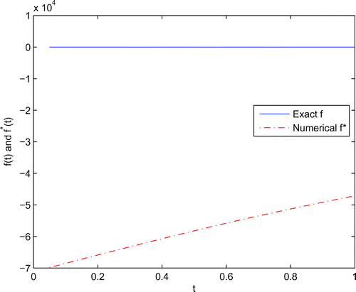
Figure 2. The GCV function obtained for various levels of noise added into the measured data, namely $\mathit{\delta }=1\%(....)$, $\mathit{\delta }=3\%(--)$ and $\mathit{\delta }=5\%(-)$, with $n=m=s=20$, $T=2.5$, $X=-1$ for Example 1.

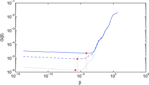
Figure 3. The analytical f(t) and its approximation $f^{\ast }(t)$ with $n=m=s=20$, $T=2.5$, $X=-1$, and various levels of noise added into the measured data, namely $\mathit{\delta }=1\%$, $\mathit{\delta }=3\%$ and $\mathit{\delta }=5\%$ for Example 1.

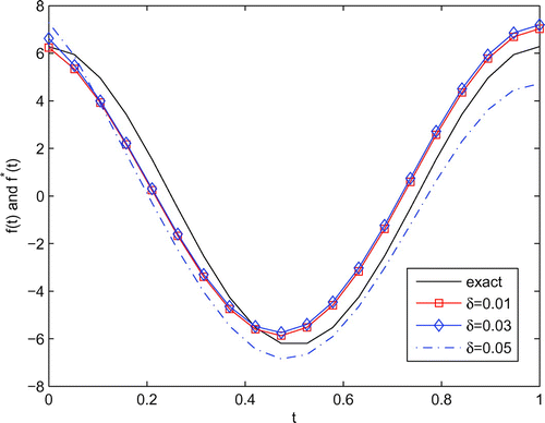
Figure 4. The analytical f(t) and its approximation $f^{\ast }(t)$ with $n=m=s=20$, $T=2.5$, $X=-1$ for fractional MFS ($\mathit{\alpha }=2$) and $n=m=s=20$, $T=2.5$ for classical MFS when level of noise added into the measured data $\mathit{\delta }=1\%$ for Example 1.

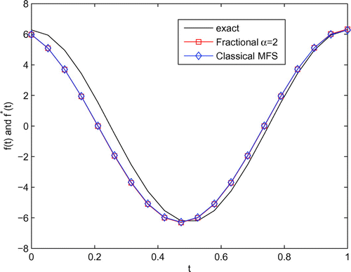
Figure 5. (a) The RMSE(f) and RRMSE(f) of the numerical solutions for Example 1 with $n=m=s=20$, $\mathit{\delta }=1\%$, $T=2.5$, $X=-1$ and $x_0=0.5$ with respect to the fractional order $\mathit{\alpha }$; (b) The RMSE(u) and RRMSE(u) of the numerical solutions for Example 1 with $n=m=s=20$, $\mathit{\delta }=1\%$, $T=2.5$, $X=-1$ and $x_0=0.5$ with respect to the fractional order $\mathit{\alpha }$; (c) The condition number cond(A) of A with $n=m=s=20$, $T=2.5$, $X=-1$ and $x_0=0.5$ with respect to the fractional order $\mathit{\alpha }$.

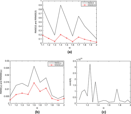
Figure 6. (a) The RMSE(u) and RRMSE(u) of the numerical solutions for Example 1 with $\mathit{\delta }=1\%$, $x_0=0.2$, $X=-1$ with respect to the parameter T; (b) The RMSE(u) and RRMSE(u) of the numerical solutions for Example 1 with $\mathit{\delta }=1\%$, $x_0=0.5$, $T=2.5$ with respect to the parameter X.

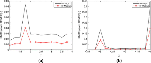
Figure 7. (a) The RMSE(f) and RRMSE(f) of the numerical solutions for Example 1 with $\mathit{\delta }=1\%$, $x_0=0.5$, $X=-1$ with respect to the parameter T; (b) The RMSE(f) and RRMSE(f) of the numerical solutions for Example 1 with $\mathit{\delta }=1\%$, $x_0=0.5$, $T=2.5$ with respect to the parameter X.

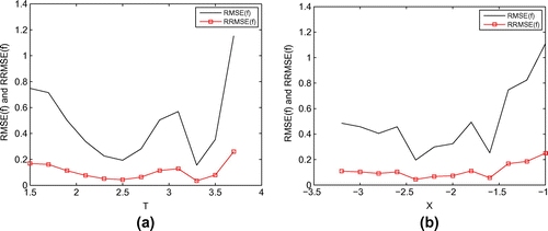
Figure 8. (a) The analytical f(t) and its approximation $f^{\ast }(t)$ with $n=m=s=25$, $T=1.5$, $X=-1$, and various levels of noise added into the measured data, namely $\mathit{\delta }=1\%$, $\mathit{\delta }=3\%$ and $\mathit{\delta }=5\%$  for  Example 2; (b) The analytical f(t) and its approximation $f^{\ast }(t)$ with $n=m=s=30$, $T=2$, $X=-1$, and various levels of noise added into the measured data,namely $\mathit{\delta }=1\%$, $\mathit{\delta }=3\%$ and $\mathit{\delta }=5\%$ for Example 2.

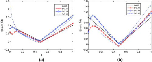
Figure 9. The GCV function obtained for various levels of noise added into the measured data, namely $\mathit{\delta }=1\%(....)$, $\mathit{\delta }=3\%(--)$ and $\mathit{\delta }=5\%(-)$, with $n=m=s=25$, $T=2.5$, $X=-1$ for Example 2.

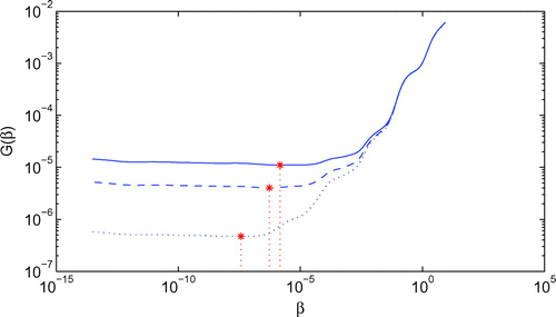
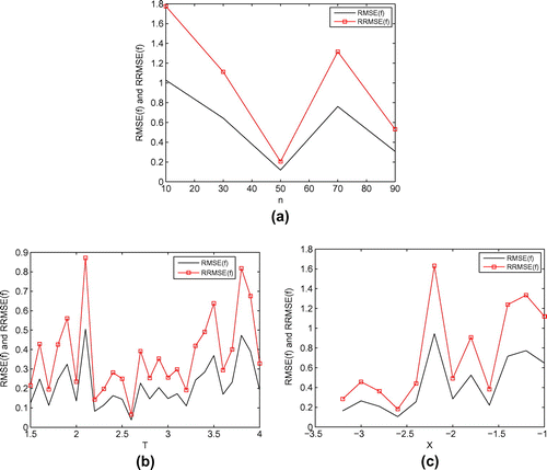
Figure 10. (a) The accuracy of the numerical solutions for Example 2 with $\mathit{\delta }=1\%,x_0=0.9,X=-1$ and $T=2.5$ with respect to the parameter n; (b) The accuracy of the numerical solutions for Example 2 with $\mathit{\delta }=1\%$, $x_0=0.9$, $X=-1$ with respect to the parameter T; (c) The accuracy of the numerical solutions for Example 2 with $\mathit{\delta }=1\%$, $x_0=0.9$, $T=1.5$ with respect to the parameter X.

From Tables 1 and 2, it can be easily observed that the Tikhonov regularization method works well. From Table 3, we will see that the closer the distance from the point $x_0$ to the regional centres is, the better the accuracy in the numerical solution is. Furthermore, the values of RMSE(f) increase as the level of noise $\mathit{\delta }$ added into the input temperature data increases. The comparison between the exact solution f(t) and the approximation $f^{\ast }(t)$ are illustrated in Figure 3, when we take $n=m=s=20$, $T=2.5$, $X=-1$ and various amounts of noise added into the data. Figure 4 displays the comparison between the analytical f(t) and its approximation $f^{\ast }(t)$ with $n=m=s=20$, $T=2.5$, $X=-1$ for fractional MFS ($\mathit{\alpha }=2$) and $n=m=s=20$, $T=2.5$ for classical MFS when level of noise added into the measured data $\mathit{\delta }=1\%$. It can be observed from this figure that the fractional MFS and the classical MFS are nearly the same, i.e. our method coincides with the classical one. Figure 5(a)–(c) display, respectively, the relationship between the accuracy of f, the accuracy of u, cond(A) and the fractional order $\mathit{\alpha }$. It is indicated that the proposed method is useful for different order $\mathit{\alpha }$, even though the condition number of $\mathbf{A}$ becomes larger and larger. Figures 6 and 7 illustrate the relationship between the accuracy of numerical solutions and the parameters T and X. It is indicated that the numerical results are not only stable with respect to parameter T and X, respectively, but also almost they maintain at the same level of accuracy over a wide range of values T and X, respectively. Thus, for the proposed method, the accuracy of numerical solutions is relatively independent of the parameter T and X, respectively. Similar conclusions can be drawn from the results for Example 2 which are shown in Figure 10.

Table 1. The values of cond(A), RMSE(u), RRMSE(u), RMSE(f), RRMSE(f) for various values of X in Example 1, $\mathit{\delta }=1\%$, $T=2.5$.

X	RMSE(u)	RRMSE(u)	RMSE(f)	RRMSE(f)	cond(A)
$X=-1$	0.5008	0.1127	0.0170	0.0083	5.9324e+18
$X=-1.3$	0.2198	0.0495	0.0091	0.0044	2.9995e+18
$X=-1.6$	0.5007	0.1127	0.0159	0.0077	2.3000e+18
$X=-2$	0.4007	0.0902	0.0102	0.0050	4.3280e+18
$X=-2.3$	0.5693	0.1281	0.0136	0.0066	2.5548e+19
$X=-2.5$	0.5898	0.1327	0.0091	0.0044	7.6651e+19

Table 2. The values of cond(A), RMSE(u), RRMSE(u), RMSE(f), RRMSE(f) for various values of T in Example 1, $\mathit{\delta }=1\%$, $X=-1$.

T	RMSE(u)	RRMSE(u)	RMSE(f)	RRMSE(f)	cond(A)
$T=1.5$	0.9622	0.2166	0.0373	0.0182	3.2758e+22
$T=1.8$	0.6423	0.1446	0.0118	0.0057	6.2945e+19
$T=2.0$	0.4672	0.1052	0.0124	0.0060	2.2338e+18
$T=2.3$	0.6369	0.1434	0.0157	0.0076	1.7224e+18
$T=2.5$	0.1999	0.0450	0.0137	0.0066	5.9324e+18
$T=2.8$	0.1358	0.0306	0.0079	0.0038	2.9637e+18

Table 3. The values of RRMSE(f) for various values of $\mathit{\delta }$ and $x_0$ in Example 1, $T=2.5$, $X=-1$.

$x_0$	$\mathit{\delta }=1\%$	$\mathit{\delta }=3\%$	$\mathit{\delta }=5\%$
$x_0=0.1$	0.2020	0.2127	0.2749
$x_0=0.2$	0.1228	0.1437	0.1687
$x_0=0.3$	0.0566	0.0859	0.1405
$x_0=0.4$	0.0480	0.0676	0.1178
$x_0=0.5$	0.0379	0.0546	0.0697
$x_0=0.6$	0.0807	0.1244	0.1481
$x_0=0.7$	0.1251	0.1435	0.1558
$x_0=0.8$	0.1405	0.1847	0.2610
$x_0=0.9$	0.1429	0.2581	0.3010

Example 2:

Consider the exact solution for problem (4(4) $$\begin{array}{c}\hfill u_t{=}_x{D}_{\mathit{\theta }}^{\mathit{\alpha }}u+f(t),0<x<1,0<t\le t_{max},\end{array}$$(4) )–(8(8) $$\begin{array}{c}\hfill u(x_0,t)=h(t),0\le t\le t_{max},\end{array}$$(8) )(49) $$\begin{array}{c}\hfill u(x,t)=\left\{\begin{array}{ccc}\hfill \frac{3}{\mathrm{\Gamma }(\mathit{\alpha }+1)}{x}^{\mathit{\alpha }}+4t-t^2,& & 0\le x\le 0.5,\hfill \\ \hfill \frac{3}{\mathrm{\Gamma }(\mathit{\alpha }+1)}{x}^{\mathit{\alpha }}+2t+t^2,& & 0.5\le x\le 1,\hfill \end{array}\right.\end{array}$$(49)

with the nonsmooth source function(50) $$\begin{array}{c}\hfill f(t)=\left\{\begin{array}{ccc}\hfill 1-2t,& & 0\le x\le 0.5,\hfill \\ \hfill 2t-1,& & 0.5\le x\le 1.\hfill \end{array}\right.\end{array}$$(50)

Throughout this example, we choose the fractional order $\mathit{\alpha }=1.9$. There are two cases in this example. In Case 1, we take $n=m=s=25$, $T=1.5$, $X=-1$ and $x_0=0.9$. The analytical function f(t) and the approximation $f^{\ast }(t)$ are displayed in Figure 8(a). In Case 2, we take $n=m=s=30$, $T=2$, $X=-1$ and $x_0=0.9$. Similar results f(t) and $f^{\ast }(t)$ are presented in Figure 8(b). From the Figure 8(a) and (b), we can observe that the numerical approximation is not so good as in the first example, but it is in reasonable agreement with (50(50) $$\begin{array}{c}\hfill f(t)=\left\{\begin{array}{ccc}\hfill 1-2t,& & 0\le x\le 0.5,\hfill \\ \hfill 2t-1,& & 0.5\le x\le 1.\hfill \end{array}\right.\end{array}$$(50) ). Figure 9 displays the regularization parameters chosen by GCV method for the results illustrated in Figure 8(a), and we can obtain the regularization parameter $\mathit{\beta }$ at ${\mathit{\beta }}^{\ast }=3.7359\text{e}-008$, ${\mathit{\beta }}^{\ast }=5.4220\text{e}-007$ and ${\mathit{\beta }}^{\ast }=1.4785\text{e}-006$ for $\mathit{\delta }=1\%$, $\mathit{\delta }=3\%$ and $\mathit{\delta }=5\%$, respectively. Similar results can be obtained for Figure 8(b), and for the sake of simplicity, they are not mentioned here. Figure 10(a) illustrates the relationship between the accuracy of f and the parameter n with the noise level $\mathit{\delta }=1\%$, $x_0=0.9$, $X=-1$ and $T=2.5$; Figure 10(b) displays the relationship between the accuracy of f and the parameter T with the noise level $\mathit{\delta }=1\%$, $x_0=0.9$, $X=-1$, where the number of collocation points is $n=m=s=25$; the relationship between the accuracy of f and the parameter X is shown in Figure 10(c) when we choose $\mathit{\delta }=1\%$, $x_0=0.9$, $T=1.5$ and $n=m=s=25$. It can be observed that our method is stable with respect to the parameters n, T and X. We can also see that the proposed method works well even if we deal with the nonsmooth numerical example.

6. Conclusions

In this article, we develop a fundamental solution method for space-fractional diffusion problem to solve an inverse time-dependent source problem of space-fractional diffusion. We adapt the Tikhonov regularization method with the GCV criterion to solve matrix Equation (35(35) $$\begin{array}{c}\hfill \mathbf{A}\mathit{\lambda }=\mathbf{b},\end{array}$$(35) ). The Green function of the space-fractional diffusion equation based on corresponding Riesz-Feller derivatives is used in our computation. The numerical results indicate that MFS technique performs well and then the accuracy of numerical solutions is relatively independent of the paraments T and X, respectively. Our technique can be extended to solve an inverse space-dependent source problem of time-fractional diffusion and this will be examined in future works. For the engineering applications, the non-trivial boundary conditions maybe have more merit. But it maybe have some difficulty to find the exact solution for such kind of problems. So, this can also be considered in the future works.

Acknowledgements

The authors gratefully thank the referees for their valuable constructive comments which improve greatly the quality of the paper.

Additional information

Funding

The work described in this article was supported by the National Natural Science Foundation of China [grant number 11326234]; Natural Science Foundation of Gansu Province [grant number 145RJZA099]; and Scientific research project of Higher School in Gansu Province [grant number 2014A-012].

Notes

No potential conflict of interest was reported by the authors.

References

- Metzler R, Klafter J. The random walk’s guide to anomalous diffusion: a fractional dynamics approach. Phys Rep. 2000;339(1):1–77. doi:10.1016/S0370-1573(00)00070-3.
- Podlubny I. Fractional differential equations: an introduction to fractional derivatives, fractional differential equations, to methods of their solution and some of their applications. San Diego (CA): Academic Press Inc.; 1999 (Mathematics in science and engineering; vol. 198).
- Scalas E, Gorenflo R, Mainardi F. Fractional calculus and continuous-time finance. Phys A. 2000;284(1–4):376–384. doi:10.1016/S0378-4371(00)00255-7.
- Chi G, Li G, Jia X. Numerical inversions of a source term in the FADE with a Dirichlet boundary condition using final observations. Comput Math Appl. 2011;62(4):1619–1626. doi:10.1016/j.camwa.2011.02.029.
- Zhang D, Li G, Chi G, et al. Numerical identification of multiparameters in the space fractional advection dispersion equation by final observations. J Appl Math. 2012;2012. 14 p. Art. ID 0740385.
- Benson DA, Wheatcraft SW, Meerschaert MM. The fractional-order governing equation of Lévy motion. Water Resour Res. 2000;36:1413–1423.
- Mera NS. The method of fundamental solutions for the backward heat conduction problem. Inverse Probl Sci Eng. 2005;13(1):65–78.
- Marin L, Lesnic D. The method of fundamental solutions for the cauchy problem in two-dimensional linear elasticity. Int J Solids Struct. 2004;41:3425–3438.
- Marin L, Lesnic D. The method of fundamental solutions for the Cauchy problem associated with two-dimensional Helmholtz-type equations. Comput Struct. 2005;83(4–5):267–278.
- Jin B, Zheng Y. A meshless method for some inverse problems associated with the Helmholtz equation. Comput Methods Appl Mech Eng. 2006;195(19–22):2270–2288.
- Hon YC, Wei T. A fundamental solution method for inverse heat conduction problem. Eng Anal Boundary Elem. 2004;28:489–495.
- Hon YC, Wei T. The method of fundamental solution for solving multidimensional inverse heat conduction problems. CMES Comput Model Eng Sci. 2005;7(2):119–132.
- Wei T, Yamamoto M. Reconstruction of a moving boundary from cauchy data in one-dimensional heat equation. Inverse Probl Sci Eng. 2009;17(4):551–567.
- Karageorghis A, Lesnic D, Marin L. A survey of applications of the MFS to inverse problems. Inverse Probl Sci Eng. 2011;19(3):309–336. doi:10.1080/17415977.2011.551830.
- Hon YC, Li M. A discrepancy principle for the source points location in using the MFS for solving the BHCP. Int J Comput Methods. 2009;6(2):181–197. doi:10.1142/S0219876209001759.
- Liu CS. The method of fundamental solutions for solving the backward heat conduction problem with conditioning by a new post-conditioner. Numer Heat Transfer Part B: Fundam. 2011;60(1):57–72.
- Wei T, Wang JC. Simultaneous determination for a space-dependent heat source and the initial data by the MFS. Eng Anal Boundary Elem. 2012;36(12):1848–1855. doi:10.1016/j.enganabound.2012.07.006.
- Chen W, Wang F. Singular boundary method using time-dependent fundamental solution for transient diffusion problems. Eng Anal Bound Elem. 2016;68:115–123. doi:10.1016/j.enganabound.2016.04.004.
- Kosec G, Šarler B. Solution of phase change problems by collocation with local pressure correction. CMES Comput Model Eng Sci. 2009;47(2):191–216.
- Šarler B, Vertnik R. Meshfree explicit local radial basis function collocation method for diffusion problems. Comput Math Appl. 2006;51(8):1269–1282. doi:10.1016/j.camwa.2006.04.013.
- Tsai CH, Young DL, Kolibal J. An analysis of backward heat conduction problems using the time evolution method of fundamental solutions. CMES Comput Model Eng Sci. 2010;66(1):53–72.
- Tsai CH, Young DL, Kolibal J. Numerical solution of three-dimensional backward heat conduction problems by the time evolution method of fundamental solutions. Int J Heat Mass Transfer. 2011;54(11):2446–2458.
- Dou FF, Hon YC. Kernel-based approximation for Cauchy problem of the time-fractional diffusion equation. Eng Anal Bound Elem. 2012;36(9):1344–1352. doi:10.1016/j.enganabound.2012.03.003.
- Dou FF, Hon YC. Numerical computation for backward time-fractional diffusion equation. Eng Anal Bound Elem. 2014;40:138–146. doi:10.1016/j.enganabound.2013.12.001.
- Dou FF, Hon YC. Fundamental kernel-based method for backward space-time fractional diffusion problem. Comput Math Appl. 2016;71(1):356–367. doi:10.1016/j.camwa.2015.11.023.
- Mainardi F, Luchko Y, Pagnini G. The fundamental solution of the space-time fractional diffusion equation. Fract Calc Appl Anal. 2001;4(2):153–192.
- Gorenflo R, Mainardi F. Some recent advances in theory and simulation of fractional diffusion processes. J Comput Appl Math. 2009;229(2):400–415. doi:10.1016/j.cam.2008.04.005.
- Gorenflo R, Mainardi F, Moretti D, et al. Fractional diffusion: probability distributions and random walk models. Phys A: Stat Mech Appl. 2002;305(1):106–112.
- Cannon JR. Determination of an unknown heat source from overspecified boundary data. SIAM J Numer Anal. 1968;5:275–286. doi:10.1137/0705024.
- Cannon JR, DuChateau P. Structural identification of an unknown source term in a heat equation. Inverse Probl. 1998;14(3):535–551. doi:10.1088/0266-5611/14/3/010.
- Savateev EG. On problems of determining the source function in a parabolic equation. J Inverse Ill-Posed Probl. 1995;3(1):83–102. doi:10.1515/jiip.1995.3.1.83.
- Farcas A, Lesnic D. The boundary-element method for the determination of a heat source dependent on one variable. J Eng Math. 2006;54(4):375–388. doi:10.1007/s10665-005-9023-0.
- Yan L, Fu CL, Yang FL. A fundamental solution method for inverse heat conduction problem. Eng Anal Boundary Elem. 2008;28:489–495.
- Wen J. A meshless method for reconstructing the heat source and partial initial temperature in heat conduction. Inverse Probl Sci Eng. 2011;19(7):1007–1022. doi:10.1080/17415977.2011.569711.
- Wen J, Yamamoto M, Wei T. Simultaneous determination of a time-dependent heat source and the initial temperature in an inverse heat conduction problem. Inverse Probl Sci Eng. 2013;21(3):485–499. doi:10.1080/17415977.2012.701626.
- Saichev AI, Zaslavsky GM. Fractional kinetic equations: solutions and applications. Chaos. 1997;7(4):753–764. doi:10.1063/1.166272.
- Hansen PC. Analysis of discrete ill-posed problems by means of the L-curve. SIAM Rev. 1992;34(4):561–580.
- Hansen PC. Numerical tools for analysis and solution of fredholm integral equations of the first kind. Inverse Probl. 1992;8(6):849–872.
- Tikhonov AN, Arsenin VY. Solutions of ill-posed problems. Washington (DC), New York (NY): V. H. Winston & Sons, Wiley; 1977. Translated from the Russian, Preface by translation editor Fritz John, Scripta Series in Mathematics.
- Hansen PC. Rank-deficient and discrete ill-posed problems. In: Flaherty JE, editor. Numerical aspects of linear inversion. SIAM monographs on mathematical modeling and computation. Philadelphia (PA): Society for Industrial and Applied Mathematics; 1998.
- Hansen PC. Regularization tools: a Matlab package for analysis and solution of discrete ill-posed problems. Numer Algorithms. 1994;6(1–2):1–35.