Numerical inversions for diffusion coefficients in two-dimensional space fractional diffusion equation

Abstract

This article deals with an inverse problem of determining the diffusion coefficients in 2D fractional diffusion equation with a Dirichlet boundary condition by the final observations at the final time. The forward problem is solved by the alternating direction implicit finite-difference scheme with the discrete of fractional derivative by shift Grünwald formula and a numerical text which is to prove its numerically stability and convergence is given. Furthermore, the homotopy regularization algorithm with the regularization parameter chosen by a Sigmoid-type function is introduced to solve the inversion problem numerically. Numerical inversions both with accurate data and noisy data are carried out for the unknown diffusion coefficients of constant and variable with polynomials, trigonometric and index functions. The reconstruction results show that the inversion algorithm is efficient for the inverse problem of determining diffusion coefficients in 2D space fractional diffusion equation, and the algorithm is also numerically stable for additional date having random noises.

Keywords:

• 2D space fractional diffusion equation
• inverse problem
• diffusion coefficient
• homotopy regularization algorithm
• numerical inversion

AMS Subject Classification:

• 65M32

View correction statement:

Erratum

1. Introduction

In recent two decades, the increasing diffusion processes were found not to obey the Fickian diffusion which could be modelled by the classical diffusion equation with second order, but fractional diffusion equation can model the phenomena preferably and provide an adequate description for these anomalous diffusion, see e.g. [1–6].

In this paper, we will deal with an inversion problem for diffusion coefficients in a homogeneous unit section $\mathrm{\Omega }=(0,1)\times (0,1)$ with final observations. The 2D fractional diffusion equation considered here is given as(1) $$\begin{array}{c}\hfill \frac{\mathit{\partial }u(x,y,t)}{\mathit{\partial }t}=D_L(x)\frac{{\mathit{\partial }}^{\mathit{\alpha }}u(x,y,t)}{\mathit{\partial }{x}^{\mathit{\alpha }}}+D_T(y)\frac{{\mathit{\partial }}^{\mathit{\beta }}u(x,y,t)}{\mathit{\partial }{y}^{\mathit{\beta }}}+f(x,y,t)\end{array}$$(1)

for $(x,y)\in \mathrm{\Omega }$ and $0<t\le T$, where $(\mathit{\alpha },\mathit{\beta })\in (1,2)$ are called space fractional orders and useful similar in application [3]. It is also the physically meaningful case, as explained in [7] and u(x, y, t) denotes the state variable at space point (x, y) and time t; $D_L(x)$ is the longitudinal diffusion coefficient, and $D_T(y)$ is the transverse diffusion coefficient; f(x, y, t) is the source/sink term. The space fractional derivative defined by Riemann-Liouville is given as follows:(2) $$\begin{array}{cc}\hfill \frac{{\mathit{\partial }}^{\mathit{\alpha }}u(x,y,t)}{\mathit{\partial }{x}^{\mathit{\alpha }}}& =\frac{1}{\mathrm{\Gamma }(2-\mathit{\alpha })}\frac{{\mathit{\partial }}^2}{\mathit{\partial }{x}^2}{\int }_0^x\frac{u(\mathit{\xi },y,t)}{{(x-\mathit{\xi })}^{(\mathit{\alpha }-1)}}\mathrm{d}\mathit{\xi }\hfill \end{array}$$(2) (3) $$\begin{array}{cc}\hfill \frac{{\mathit{\partial }}^{\mathit{\beta }}u(x,y,t)}{\mathit{\partial }{y}^{\mathit{\beta }}}& =\frac{1}{\mathrm{\Gamma }(2-\mathit{\beta })}\frac{{\mathit{\partial }}^2}{\mathit{\partial }{y}^2}{\int }_0^y\frac{u(x,\mathit{\eta },t)}{{(y-\mathit{\eta })}^{(\mathit{\beta }-1)}}\mathrm{d}\mathit{\eta }\hfill \end{array}$$(3)

Here $\mathrm{\Gamma }$ is the gamma function. See e.g. [8,9] for the definitions and properties of fractional derivatives. There are accurate methods and numerical methods for solving the fractional diffusion equation, such as collocation method [10,11], tau method [12,13], operational formulation of spectral techniques [13,14], element free Galerkin method [15], mesh-free methods [16–18], finite-differential scheme [19–21], finite element and singular boundary method [22,23].

Quite a few of researches have been carried out on the development of numerical methods for 2D fractional diffusion equations with the application of fractional calculus and derivatives in science and engineering. Meerschaert et al. [24] firstly studied the numerically method for two-dimensional space fractional dispersion equation and gave a finite-difference method with the classical alternating-direction method and proved the unconditionally stability of the method. Chen et al. [25] gave an implicit numerical method for the two-dimensional fractional percolation equation without the assumption of continued and rigid body motion and proved its consistency, stability and convergence and gave some numerical examples to demonstrate the effectiveness of the theoretical analysis. Wang and Wang [26] presented an alternating-direction finite-difference method for two-dimensional fractional diffusion equation with Toeplitz matrices and fast Fourier transform and gave demonstration for its method which is supported by numerical examples. Li et al. [27] presented an alternating direction implicit-Eluer method for the two-dimensional fractional evolution.

In recent years, spectral techniques become a popular method in dealing with fractional diffusion equation. Bhrawy [10] adapted an operational matrix formulation of the collocation method for the one and two-dimensional non-linear fractional sub diffusion equations (FSDEs). Bhrawy and Baleanu [28] applied an efficient Legendre–Gauss–Lobatto collocation (L-GL-C) method which reduced the problem to the solution of a system of ordinary differential equations in time to solve the space fractional advection diffusion equation with nonhomogeneous initial-boundary conditions. Doha [29] proposed an accurate and efficient spectral tau technique for solving the fractional diffusion equations numerically. Huang and Zheng [30] presented a numerical scheme for space fractional diffusion equations (SFDEs) based on pseudo-spectral method which is reduced to a system of ordinary differential equations for time variable t. Li and Xu [31] constructed an efficient spectral method for numerical approximations of the weak solution for the space-time fractional diffusion equation based on the proposed weak formulation. Li and Xu [32] proposed a spectral method in both temporal and spatial discretizations for the time-fractional diffusion equation and gave numerical texts. Bueno et al. [33] introduced Fourier spectral methods as an attractive and easy-to-code alternative for the integration of fractional-in-space reaction-diffusion equations described by the fractional Laplacian in bounded rectangular domains of $R^n$.

As we know, some important parameters such as the diffusion coefficients in Equation (1(1) $$\begin{array}{c}\hfill \frac{\mathit{\partial }u(x,y,t)}{\mathit{\partial }t}=D_L(x)\frac{{\mathit{\partial }}^{\mathit{\alpha }}u(x,y,t)}{\mathit{\partial }{x}^{\mathit{\alpha }}}+D_T(y)\frac{{\mathit{\partial }}^{\mathit{\beta }}u(x,y,t)}{\mathit{\partial }{y}^{\mathit{\beta }}}+f(x,y,t)\end{array}$$(1) ) in real problem are always unknown and cannot be measured directly but can be determined from some additional information indirectly which always lead to the inverse problem. To our knowledge, the research on inverse problems in the fractional diffusion equation has not been paid much attention. In [34–36], conditional stability for Cauchy problems in some time-fractional diffusion equations was analysed, and in [37–41], inverse problems of identifying source terms or source coefficients in the time/space fractional diffusion equations were studied by regularization methodology, and in [42,43], numerical inversions for determining source terms in the space fractional diffusion equation were performed using the optimal perturbation algorithm. For the diffusion coefficients inversion problem in 2D diffusion equation, Zhang et al. [44] studied an inverse problem of simultaneously determining the dispersion coefficient and the space-dependent source magnitude in 2D advection dispersion equation and presented some effective numerical inversion by the optimal perturbation algorithm with the regularization parameter chosen by a sigmoid function.

For the inverse problem of determining diffusion coefficients in 1D fractional diffusion equation, Cheng et al. [45] studied an inverse problem of determining the space-dependent diffusion coefficient and fractional order with in formal initial condition, and proved the uniqueness of the inverse problem with Gel’fand-Levitan theory and eigenfunction expansion. Similar to [45], Li and Yamamoto et al. [46] considered an inverse problem of identifying the space-depended diffusion coefficient and fractional order with continuous initial condition and proved the uniqueness of the inverse problem and given effective numerical inversion examples. Li et al. [47] also studied the inverse problem of determining the space-dependent diffusion coefficient and the source magnitude in 1D time-fractional diffusion, and presented some numerical inversions by optimal perturbation algorithm. In addition, there are some literatures which deal with the inverse problem of diffusion equation like, spectral collocation algorithm [48], homotopy perturbation method [49], tau method [50].

For Equation (1(1) $$\begin{array}{c}\hfill \frac{\mathit{\partial }u(x,y,t)}{\mathit{\partial }t}=D_L(x)\frac{{\mathit{\partial }}^{\mathit{\alpha }}u(x,y,t)}{\mathit{\partial }{x}^{\mathit{\alpha }}}+D_T(y)\frac{{\mathit{\partial }}^{\mathit{\beta }}u(x,y,t)}{\mathit{\partial }{y}^{\mathit{\beta }}}+f(x,y,t)\end{array}$$(1) ), what we want to do is to determine the diffusion coefficients using the inversion algorithm. For the forward problem, we still utilize the classical alternating-direction method and give some numerical examples to test the stability of the differential scheme. The inversion problem here for simultaneously identifying the longitudinal diffusion coefficient and transverse diffusion coefficient becomes severely ill-posed in 2D fractional diffusion equation. The ordinary optimal perturbation algorithm used in [42,51] and regularization algorithm [52,53] cannot be modified for the inversion problem. We employ the homotopy regularization algorithm as studied in [44] and [54,55]. Furthermore, some numerical examples are presented and several important factors in the inversion algorithm are discussed, such as numerical differential step, additional data and fractional order, etc. The numerical inversion with random noisy data is also discussed and the inversion solution gives good approximation to the exact solution as the noise level becomes small.

The rest of the paper is arranged as follows.

In Section 2, an alternative-direction difference scheme for solving the forward problem is deduced, and its stability is given, and two numerical examples are presented to support the difference method. In Section 3, an inverse problem of determining the diffusion coefficients in Equation (1(1) $$\begin{array}{c}\hfill \frac{\mathit{\partial }u(x,y,t)}{\mathit{\partial }t}=D_L(x)\frac{{\mathit{\partial }}^{\mathit{\alpha }}u(x,y,t)}{\mathit{\partial }{x}^{\mathit{\alpha }}}+D_T(y)\frac{{\mathit{\partial }}^{\mathit{\beta }}u(x,y,t)}{\mathit{\partial }{y}^{\mathit{\beta }}}+f(x,y,t)\end{array}$$(1) ) is formulated, and the homotopy regularization algorithm with sigmoid-type regularization parameter is given. In Sections 4 and 5, numerical inversions with accurate data and noisy data are carried out, and the factors having important influences on the inversion algorithm are discussed. Finally, several concluding remarks are given in Section 6.

2. The forward problem and ADI scheme

2.1. The forward problem

Considering the numerical solution for Equation (1(1) $$\begin{array}{c}\hfill \frac{\mathit{\partial }u(x,y,t)}{\mathit{\partial }t}=D_L(x)\frac{{\mathit{\partial }}^{\mathit{\alpha }}u(x,y,t)}{\mathit{\partial }{x}^{\mathit{\alpha }}}+D_T(y)\frac{{\mathit{\partial }}^{\mathit{\beta }}u(x,y,t)}{\mathit{\partial }{y}^{\mathit{\beta }}}+f(x,y,t)\end{array}$$(1) ) with the initial condition(4) $$\begin{array}{c}\hfill u(x,y,0)=u_0(x,y)\end{array}$$(4)

and the boundary conditions(5) $$\begin{array}{c}\hfill u(0,y,t)=0,u(1,y,t)=0,u(x,0,t)=0,u(x,1,t)=0\end{array}$$(5)

Suppose that there is a classical solution $u=u(x,y,t)$ defined in the domain $\overline{{\mathrm{\Omega }}_T}=\mathrm{\Omega }\times [0,T]$ which satisfies the Equation (1(1) $$\begin{array}{c}\hfill \frac{\mathit{\partial }u(x,y,t)}{\mathit{\partial }t}=D_L(x)\frac{{\mathit{\partial }}^{\mathit{\alpha }}u(x,y,t)}{\mathit{\partial }{x}^{\mathit{\alpha }}}+D_T(y)\frac{{\mathit{\partial }}^{\mathit{\beta }}u(x,y,t)}{\mathit{\partial }{y}^{\mathit{\beta }}}+f(x,y,t)\end{array}$$(1) ) and the initial boundary conditions and belongs to the space $C(\overline{{\mathrm{\Omega }}_T})\cap W^1[0,T]\cap C(\mathrm{\Omega })$. Where $W^1[0,T]$ is the space of the function $h(t)\in C^1[0,T]$ and $h^{{}^{\prime }}(t)\in L[0,T]$. Furthermore, the longitudinal diffusion coefficients $D_L(x)$, the transverse diffusion coefficient $D_T(y)$, the source term f(x, y, t), and the initial condition $u_0(x,y)$ have to belong to the spaces C[0, 1], C[0, 1], $C(\overline{{\mathrm{\Omega }}_T})$ and $C(\mathrm{\Omega })$, respectively. If all the above parameters are known, the problem (1(1) $$\begin{array}{c}\hfill \frac{\mathit{\partial }u(x,y,t)}{\mathit{\partial }t}=D_L(x)\frac{{\mathit{\partial }}^{\mathit{\alpha }}u(x,y,t)}{\mathit{\partial }{x}^{\mathit{\alpha }}}+D_T(y)\frac{{\mathit{\partial }}^{\mathit{\beta }}u(x,y,t)}{\mathit{\partial }{y}^{\mathit{\beta }}}+f(x,y,t)\end{array}$$(1) ), (4(4) $$\begin{array}{c}\hfill u(x,y,0)=u_0(x,y)\end{array}$$(4) )–(5(5) $$\begin{array}{c}\hfill u(0,y,t)=0,u(1,y,t)=0,u(x,0,t)=0,u(x,1,t)=0\end{array}$$(5) ) is called the forward problem. We give the numerical method of the forward problem by utilizing shift Grünwald formula and alternating direction implicit (ADI) finite-difference scheme.

Denote the grid points in the space domain $\mathrm{\Omega }$ as $x_i=i{h}_x,(i=0,1,2,\dots ,N_x),y_j=j{h}_y,(j=0,1,2,\dots ,N_y)$ with the space step size $h_x=1/N_x$ and $h_y=1/N_y$, and the grid points in time interval [0, T] are labeled as $t_n=n\mathit{\tau },(n=0,1,\dots ,N)$ with $N_x,N_y$ and N be positive integers. The value of function u(x, y, t) at the grid points are denote as $u_{i,j}^n=u(x_i,y_j,t_n)$.

Based on the shift Grünwald formula the space fractional derivative $\frac{{\mathit{\partial }}^{\mathit{\alpha }}u(x,y,t)}{\mathit{\partial }{x}^{\mathit{\alpha }}}$ and $\frac{{\mathit{\partial }}^{\mathit{\beta }}u(x,y,t)}{\mathit{\partial }{y}^{\mathit{\beta }}}$ can be defined as follows (see e.g.[9])(6) $$\begin{array}{cc}\hfill \frac{{\mathit{\partial }}^{\mathit{\alpha }}u(x,y,t)}{\mathit{\partial }{x}^{\mathit{\alpha }}}{|}_{i,j}^{n+1}& =\frac{1}{h_x^{\mathit{\alpha }}}\sum _{k=0}^{i+1}{g}_k^{(\mathit{\alpha })}{u}_{i-k+1,j}^{n+1}+O(h_x)\hfill \end{array}$$(6) (7) $$\begin{array}{cc}\hfill \frac{{\mathit{\partial }}^{\mathit{\beta }}u(x,y,t)}{\mathit{\partial }{y}^{\mathit{\beta }}}{|}_{i,j}^{n+1}& =\frac{1}{h_y^{\mathit{\beta }}}\sum _{k=0}^{j+1}{g}_k^{(\mathit{\beta })}{u}_{i,j-k+1}^{n+1}+O(h_y),\hfill \end{array}$$(7)

where $g_k^{(\mathit{\lambda })}=\frac{\mathrm{\Gamma }(k-\mathit{\lambda })}{\mathrm{\Gamma }(-\mathit{\lambda })\mathrm{\Gamma }(k+1)}$ is the fractional expansion coefficient and is satisfied the following properties [9,24,56](8) $$\begin{array}{c}\hfill g_0^{(\mathit{\lambda })}=1,g_1^{(\mathit{\lambda })}=-\mathit{\lambda },1\ge g_2^{(\mathit{\lambda })}\ge g_3^{(\mathit{\lambda })}\ge \cdots \ge 0,\sum _{k=0}^{\infty }{g}_k^{(\mathit{\lambda })}=0,\sum _{k=0}^m{g}_k^{(\mathit{\lambda })}\le 0(m\ge 1)\end{array}$$(8)

If considering classical difference method and the time derivative can be instead of one order difference, the scheme is(9) $$\begin{array}{c}\hfill \frac{u_{i,j}^{n+1}-u_{i,j}^n}{\mathit{\tau }}=\frac{D_L(x_i)}{h_x^{\mathit{\alpha }}}\sum _{k=0}^{i+1}{g}_k^{(\mathit{\alpha })}{u}_{i-k+1,j}^{n+1}+\frac{D_T(y_j)}{h_y^{\mathit{\beta }}}\sum _{k=0}^{j+1}{g}_k^{(\mathit{\beta })}{u}_{i,j-k+1}^{n+1}+f_{i,j}^{n+1}\end{array}$$(9)

It can be rewritten to the implicit difference scheme as(10) $$\begin{array}{c}\hfill u_{i,j}^{n+1}-\frac{\mathit{\tau }{D}_L(x_i)}{h_x^{\mathit{\alpha }}}\sum _{k=0}^{i+1}{g}_k^{(\mathit{\alpha })}{u}_{i-k+1,j}^{n+1}-\frac{\mathit{\tau }{D}_T(y_j)}{h_y^{\mathit{\beta }}}\sum _{k=0}^{j+1}{g}_k^{(\mathit{\beta })}{u}_{i,j-k+1}^{n+1}=u_{i,j}^n+\mathit{\tau }{f}_{i,j}^{n+1}\end{array}$$(10)

Because of its high computational complexity, it is difficult to compute by above scheme (10(10) $$\begin{array}{c}\hfill u_{i,j}^{n+1}-\frac{\mathit{\tau }{D}_L(x_i)}{h_x^{\mathit{\alpha }}}\sum _{k=0}^{i+1}{g}_k^{(\mathit{\alpha })}{u}_{i-k+1,j}^{n+1}-\frac{\mathit{\tau }{D}_T(y_j)}{h_y^{\mathit{\beta }}}\sum _{k=0}^{j+1}{g}_k^{(\mathit{\beta })}{u}_{i,j-k+1}^{n+1}=u_{i,j}^n+\mathit{\tau }{f}_{i,j}^{n+1}\end{array}$$(10) ). Then, we will modify the scheme (10(10) $$\begin{array}{c}\hfill u_{i,j}^{n+1}-\frac{\mathit{\tau }{D}_L(x_i)}{h_x^{\mathit{\alpha }}}\sum _{k=0}^{i+1}{g}_k^{(\mathit{\alpha })}{u}_{i-k+1,j}^{n+1}-\frac{\mathit{\tau }{D}_T(y_j)}{h_y^{\mathit{\beta }}}\sum _{k=0}^{j+1}{g}_k^{(\mathit{\beta })}{u}_{i,j-k+1}^{n+1}=u_{i,j}^n+\mathit{\tau }{f}_{i,j}^{n+1}\end{array}$$(10) ) and give the ADI difference scheme as follows.

2.2. The ADI scheme

The idea of the ADI method is to split the scheme (10(10) $$\begin{array}{c}\hfill u_{i,j}^{n+1}-\frac{\mathit{\tau }{D}_L(x_i)}{h_x^{\mathit{\alpha }}}\sum _{k=0}^{i+1}{g}_k^{(\mathit{\alpha })}{u}_{i-k+1,j}^{n+1}-\frac{\mathit{\tau }{D}_T(y_j)}{h_y^{\mathit{\beta }}}\sum _{k=0}^{j+1}{g}_k^{(\mathit{\beta })}{u}_{i,j-k+1}^{n+1}=u_{i,j}^n+\mathit{\tau }{f}_{i,j}^{n+1}\end{array}$$(10) ) into two parts, one with the x-derivative taken implicitly and the other with the y-derivative taken implicitly by drawing into the intermediate layer $t_{n+1/2}$ between $t_n$ and $t_{n+1}$, and the scheme (10(10) $$\begin{array}{c}\hfill u_{i,j}^{n+1}-\frac{\mathit{\tau }{D}_L(x_i)}{h_x^{\mathit{\alpha }}}\sum _{k=0}^{i+1}{g}_k^{(\mathit{\alpha })}{u}_{i-k+1,j}^{n+1}-\frac{\mathit{\tau }{D}_T(y_j)}{h_y^{\mathit{\beta }}}\sum _{k=0}^{j+1}{g}_k^{(\mathit{\beta })}{u}_{i,j-k+1}^{n+1}=u_{i,j}^n+\mathit{\tau }{f}_{i,j}^{n+1}\end{array}$$(10) ) can be improved from $t_n$ to $t_{n+1/2}$, there is(11) $$\begin{array}{c}\hfill u_{i,j}^{n+1/2}-\frac{\mathit{\tau }{D}_L(x_i)}{h_x^{\mathit{\alpha }}}\sum _{k=0}^{i+1}{g}_k^{(\mathit{\alpha })}{u}_{i-k+1,j}^{n+1/2}=u_{i,j}^n+\mathit{\tau }{f}_{i,j}^{n+1}\end{array}$$(11)

and from $t_{n+1/2}$ to $t_{n+1}$, we have(12) $$\begin{array}{c}\hfill u_{i,j}^{n+1}-\frac{\mathit{\tau }{D}_T(y_j)}{h_y^{\mathit{\beta }}}\sum _{k=0}^{j+1}{g}_k^{(\mathit{\beta })}{u}_{i,j-k+1}^{n+1}=u_{i,j}^{n+1/2}\end{array}$$(12)

Denote $U^n={[u_{1,1}^n,u_{2,1}^n,\dots ,u_{N_x-1,1}^n,\dots ,u_{1,2}^n,u_{2,2}^n,\dots ,u_{N_x-1,2}^n,\dots ,u_{1,N_y-1}^n,\dots ,u_{N_x-1,N_y-1}^n]}^T,p_i=\frac{\mathit{\tau }{D}_L(x_i)}{h_x^{\mathit{\alpha }}},q_j=\frac{\mathit{\tau }{D}_T(y_j)}{h_y^{\mathit{\beta }}}$, the scheme (11(11) $$\begin{array}{c}\hfill u_{i,j}^{n+1/2}-\frac{\mathit{\tau }{D}_L(x_i)}{h_x^{\mathit{\alpha }}}\sum _{k=0}^{i+1}{g}_k^{(\mathit{\alpha })}{u}_{i-k+1,j}^{n+1/2}=u_{i,j}^n+\mathit{\tau }{f}_{i,j}^{n+1}\end{array}$$(11) ) and (12(12) $$\begin{array}{c}\hfill u_{i,j}^{n+1}-\frac{\mathit{\tau }{D}_T(y_j)}{h_y^{\mathit{\beta }}}\sum _{k=0}^{j+1}{g}_k^{(\mathit{\beta })}{u}_{i,j-k+1}^{n+1}=u_{i,j}^{n+1/2}\end{array}$$(12) ) can be rewritten as matrix form(13) $$\begin{array}{cc}\hfill A{U}_{i,j}^{n+1/2}& =U_{i,j}^n+\mathit{\tau }{f}_{i,j}^{n+1}\hfill \end{array}$$(13) (14) $$\begin{array}{cc}\hfill B{U}_{i,j}^{n+1}& =U_{i,j}^{n+1/2}\hfill \end{array}$$(14)

where $A={(a_{i,j})}_{(N_x-1)\times (N_x-1)}$ and $B={(b_{i,j})}_{(N_y-1)\times (N_y-1)}$(15) $$\begin{array}{cc}\hfill a_{\mathit{ij}}& =\left\{\begin{array}{c}-p_i{g}_{i-j+1}^{(\mathit{\alpha })},\\ 1-p_i{g}_1^{(\mathit{\alpha })},\\ -p_i,\\ 0,\end{array}\right.\begin{array}{c}\text{if}\\ \text{if}\\ \text{if}\\ \text{if}\end{array}\begin{array}{c}j\le i-1,\\ j=i,\\ j=i+1,\\ j>i+1,\end{array}\hfill \end{array}$$(15) (16) $$\begin{array}{cc}\hfill b_{\mathit{ij}}& =\left\{\begin{array}{c}-q_j{g}_{j-i+1}^{(\mathit{\beta })},\\ 1-q_j{g}_1^{(\mathit{\beta })},\\ -q_j,\\ 0,\end{array}\right.\begin{array}{c}\text{if}\\ \text{if}\\ \text{if}\\ \text{if}\end{array}\begin{array}{c}i\le j-1,\\ i=j,\\ i=j+1,\\ i>j+1,\end{array}\hfill \end{array}$$(16)

Therefore, we can solve the scheme (13(13) $$\begin{array}{cc}\hfill A{U}_{i,j}^{n+1/2}& =U_{i,j}^n+\mathit{\tau }{f}_{i,j}^{n+1}\hfill \end{array}$$(13) ) and (14(14) $$\begin{array}{cc}\hfill B{U}_{i,j}^{n+1}& =U_{i,j}^{n+1/2}\hfill \end{array}$$(14) ) instead of Equation (1(1) $$\begin{array}{c}\hfill \frac{\mathit{\partial }u(x,y,t)}{\mathit{\partial }t}=D_L(x)\frac{{\mathit{\partial }}^{\mathit{\alpha }}u(x,y,t)}{\mathit{\partial }{x}^{\mathit{\alpha }}}+D_T(y)\frac{{\mathit{\partial }}^{\mathit{\beta }}u(x,y,t)}{\mathit{\partial }{y}^{\mathit{\beta }}}+f(x,y,t)\end{array}$$(1) ). For the above difference scheme, similarly as done in [24,56], it is not difficult to get its convergence and stability by spectrum analysis to the coefficient matrix.

Lemma 2.1:

[see [24]] The implicit difference scheme defined by (13(13) $$\begin{array}{cc}\hfill A{U}_{i,j}^{n+1/2}& =U_{i,j}^n+\mathit{\tau }{f}_{i,j}^{n+1}\hfill \end{array}$$(13) ) and (14(14) $$\begin{array}{cc}\hfill B{U}_{i,j}^{n+1}& =U_{i,j}^{n+1/2}\hfill \end{array}$$(14) ) to the forward problem with $1<\mathit{\alpha },\mathit{\beta }<2$ is unconditionally stable and the difference solution is convergent to the exact solution of the forward problem with the rate $O(h_x,h_y,\mathit{\tau })$.

2.3. Numerical testification

In this subsection, two examples with constant and variable diffusion coefficients are presented to show effectiveness of the finite-difference scheme for solving the forward problem numerically.

If the diffusion coefficient is constant, set $D_L(x)=1$, $D_T(y)=1$, $f(x,y,t)=[-x(1-x)y(1-y)-y(1-y)(\frac{1-\mathit{\alpha }}{\mathrm{\Gamma }(2-\mathit{\alpha })}-\frac{2x^{2-\mathit{\alpha }}}{\mathrm{\Gamma }(3-\mathit{\alpha })})-x(1-x)(\frac{1-\mathit{\beta }}{\mathrm{\Gamma }(2-\mathit{\beta })}-\frac{2y^{2-\mathit{\beta }}}{\mathrm{\Gamma }(3-\mathit{\beta })})]e^{-t}$, the exact solution of the forward problem can be obtained which is given as $u(x,y,t)=x(1-x)y(1-y)e^{-t}$. Denote numerical solution being $u^{\ast }(x,y,t)$, the solution error can be defined by $Err=\frac{\Vert u-u^{\ast }{\Vert }_2}{\Vert u{\Vert }_2}$, CPU(s) is the computational time in calculating one time for the computer. We use the computer of Lenovo G480A-ISE which CPU type is Intel core i7 with 2.9 GH and memory size is 4 GB. 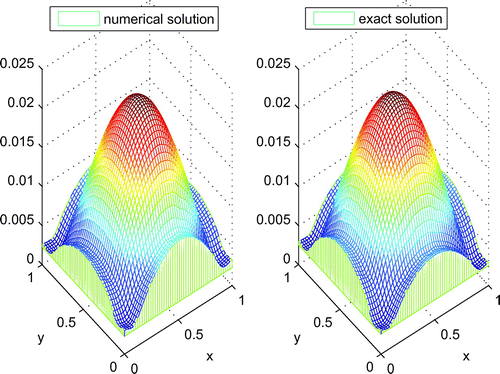Taking $\mathit{\alpha }=1.9,\mathit{\beta }=1.9,T=1$, numerical results with mesh step are listed in Tables 1–3 and Figure 1, respectively, where $N_x$, $N_y$, N denotes the number of space and time grids, respectively. Taking $N=320$, the impacts of fractional order for the direction solution is listed in Table 4.

Table 1. Impacts of mesh steps for direct solution.

$N_x=N_y=N$	10	20	40	80	160
Err	0.3047	0.1782	0.1011	0.0647	0.0434
CPU(s)	0.09	0.59	8.85	162.21	3388.48

Table 2. Impacts of space mesh steps for direct solution.

$N_x=N_y(N=80)$	10	20	40	80
Err	0.0684	0.0664	0.0652	0.0647
CPU(s)	0.34	2.32	18.13	162.21

Table 3. Impacts of time mesh steps for direct solution.

$N(N_x=N_y=10)$	10	20	40	80	160	320
Err	0.3047	0.1816	0.1062	0.0684	0.0426	0.0378
CPU(s)	0.09	0.13	0.20	0.32	0.68	1.2

Table 4. Impacts of fractional order for direct solution.

$\mathit{\alpha }(\mathit{\beta }=1.9)$	Err	$\mathit{\beta }(\mathit{\alpha }=1.9)$	Err
1.1	0.0868	1.1	0.0901
1.2	0.0811	1.2	0.0834
1.3	0.0740	1.3	0.0763
1.4	0.0659	1.4	0.0671
1.5	0.0579	1.5	0.0581
1.6	0.0509	1.6	0.0512
1.7	0.0464	1.7	0.0467
1.8	0.0458	1.8	0.0450
1.9	0.0378	1.9	0.0378

Figure 1. The comparison of the numerical solution and exact solution in case of $N_x=N_y=10,N=320$.

From Tables 1–3, we can see that the solution is convergence numerically with the mesh step to 0 and the major factor for the error is the time mesh step. From Table 4, we can see that with the space fractional order tending to 2, the solution error become small and the fractional derivative have little influence on the directed solution. From Figure 1, we find that the numerical solution is good agreement with the exact solution if $\mathit{\alpha }=\mathit{\beta }=1.9$ and $N_x=N_y=10,N=320$.

If the diffusion coefficients is variable, set $D_L(x)=x^{\mathit{\alpha }}$, $D_T(y)=y^{\mathit{\beta }}$, $f(x,y,t)=[(-x(1-x)-(\frac{\mathit{\alpha }}{\mathrm{\Gamma }(2-\mathit{\alpha })}-\frac{2\mathit{\alpha }x}{\mathrm{\Gamma }(3-\mathit{\alpha })})-(\frac{1}{\mathrm{\Gamma }(1-\mathit{\alpha })}-\frac{2x}{\mathrm{\Gamma }(2-\mathit{\alpha })})]y(1-y)e^{-t}-[(\frac{\mathit{\beta }}{\mathrm{\Gamma }(2-\mathit{\beta })}-\frac{2\mathit{\beta }y}{\mathrm{\Gamma }(3-\mathit{\alpha })})-(\frac{1}{\mathrm{\Gamma }(1-\mathit{\beta })}-\frac{2y}{\mathrm{\Gamma }(2-\mathit{\beta })})]x(1-x)e^{-t}$, the exact solution of the forward problem can be obtained which is given as $u(x,y,t)=x(1-x)y(1-y)e^{-t}$. Taking $\mathit{\alpha }=1.9$, $\mathit{\beta }=1.9$, $T=1$, the numerical results are listed in Table 5.

Table 5. Impacts of mesh steps for direct solution.

$N=320(N_x=N_y=10)$	10	20	40	80	160
Err	0.2847	0.1542	0.0868	0.0641	0.0343

From Table 5, we can see that the numerical solution is good agreement with the exact solution for variable diffusion coefficients. We can derive that the ADI difference scheme given by (13(13) $$\begin{array}{cc}\hfill A{U}_{i,j}^{n+1/2}& =U_{i,j}^n+\mathit{\tau }{f}_{i,j}^{n+1}\hfill \end{array}$$(13) ) and (14(14) $$\begin{array}{cc}\hfill B{U}_{i,j}^{n+1}& =U_{i,j}^{n+1/2}\hfill \end{array}$$(14) ) is of numerically convergence. In follows, numerical inversions for diffusion coefficients can be performed based on the above numerical method.

3. The inverse problem and inversion algorithm

3.1. The inverse problem

As we know, some parameters are often unknown and cannot be measured easily in many real problem with the anomalous diffusion model given by Equation (1(1) $$\begin{array}{c}\hfill \frac{\mathit{\partial }u(x,y,t)}{\mathit{\partial }t}=D_L(x)\frac{{\mathit{\partial }}^{\mathit{\alpha }}u(x,y,t)}{\mathit{\partial }{x}^{\mathit{\alpha }}}+D_T(y)\frac{{\mathit{\partial }}^{\mathit{\beta }}u(x,y,t)}{\mathit{\partial }{y}^{\mathit{\beta }}}+f(x,y,t)\end{array}$$(1) ), such as the fractional order, the diffusion coefficients and so on. However, the parameters like diffusion coefficients can be identified from some additional dada which can be observed by the forward problem. The problem of obtaining the unknown parameters can be regarded as an inverse problem. Suppose that the fractional order $\mathit{\alpha }$ and $\mathit{\beta }$, the diffusion coefficients $D_L(x)$ and $D_T(y)$, the source term f(x, y, t) in Equation (1(1) $$\begin{array}{c}\hfill \frac{\mathit{\partial }u(x,y,t)}{\mathit{\partial }t}=D_L(x)\frac{{\mathit{\partial }}^{\mathit{\alpha }}u(x,y,t)}{\mathit{\partial }{x}^{\mathit{\alpha }}}+D_T(y)\frac{{\mathit{\partial }}^{\mathit{\beta }}u(x,y,t)}{\mathit{\partial }{y}^{\mathit{\beta }}}+f(x,y,t)\end{array}$$(1) ) are all known, we can obtain the final observation at final time T as the additional data given as(17) $$\begin{array}{c}\hfill u(x,y,T)={\mathit{\theta }}_T(x,y),(x,y)\in \mathrm{\Omega }\end{array}$$(17)

Then, an inverse problem of determining these two parameters $D_L(x)$ and $D_T(y)$ is formulated by (1(1) $$\begin{array}{c}\hfill \frac{\mathit{\partial }u(x,y,t)}{\mathit{\partial }t}=D_L(x)\frac{{\mathit{\partial }}^{\mathit{\alpha }}u(x,y,t)}{\mathit{\partial }{x}^{\mathit{\alpha }}}+D_T(y)\frac{{\mathit{\partial }}^{\mathit{\beta }}u(x,y,t)}{\mathit{\partial }{y}^{\mathit{\beta }}}+f(x,y,t)\end{array}$$(1) ), (4(4) $$\begin{array}{c}\hfill u(x,y,0)=u_0(x,y)\end{array}$$(4) ), (5(5) $$\begin{array}{c}\hfill u(0,y,t)=0,u(1,y,t)=0,u(x,0,t)=0,u(x,1,t)=0\end{array}$$(5) ) and (17(17) $$\begin{array}{c}\hfill u(x,y,T)={\mathit{\theta }}_T(x,y),(x,y)\in \mathrm{\Omega }\end{array}$$(17) ). Actually for real problems, we could obtain a finite number of the measured data as the additional information, given at $(x_l,y_m)$ for $l=1,2,\dots ,L$ and $m=1,2,\dots ,M$, Thus the real additional data for solving the inverse problem are given as(18) $$\begin{array}{c}\hfill u(x_l,y_m,T)={\mathit{\theta }}_T(x_l,y_m),(x,y)\in \mathrm{\Omega },l=1,2,\dots ,L,m=1,2,\dots ,M\end{array}$$(18)

What we want to do follows is to solve the diffusion coefficient inversion problem of the real additional data (18(18) $$\begin{array}{c}\hfill u(x_l,y_m,T)={\mathit{\theta }}_T(x_l,y_m),(x,y)\in \mathrm{\Omega },l=1,2,\dots ,L,m=1,2,\dots ,M\end{array}$$(18) ) and the model (1(1) $$\begin{array}{c}\hfill \frac{\mathit{\partial }u(x,y,t)}{\mathit{\partial }t}=D_L(x)\frac{{\mathit{\partial }}^{\mathit{\alpha }}u(x,y,t)}{\mathit{\partial }{x}^{\mathit{\alpha }}}+D_T(y)\frac{{\mathit{\partial }}^{\mathit{\beta }}u(x,y,t)}{\mathit{\partial }{y}^{\mathit{\beta }}}+f(x,y,t)\end{array}$$(1) ) and (4(4) $$\begin{array}{c}\hfill u(x,y,0)=u_0(x,y)\end{array}$$(4) )–(5(5) $$\begin{array}{c}\hfill u(0,y,t)=0,u(1,y,t)=0,u(x,0,t)=0,u(x,1,t)=0\end{array}$$(5) ) from the view point of numerical identification by the forward problem.

3.2. The inversion algorithm

Suppose that both ${\mathrm{\Phi }}_1\subset C[0,1]$ and ${\mathrm{\Phi }}_2\subset C[0,1]$ are the admissible sets for the longitudinal diffusion coefficients $D_L(x)$ and the transverse diffusion coefficient $D_T(y)$. A solution to the inverse problem can be represented by $<D_L(x),D_T(y)>\in {\mathrm{\Phi }}_1\times {\mathrm{\Phi }}_2$. For any prescribed $D_L(x)\in {\mathrm{\Phi }}_1,D_T(y)\in {\mathrm{\Phi }}_2$, the solution of the corresponding forward problem which is denoted by $u(x,y,T;D_L(x),D_T(y))$ can be solved by the ADI difference scheme (13(13) $$\begin{array}{cc}\hfill A{U}_{i,j}^{n+1/2}& =U_{i,j}^n+\mathit{\tau }{f}_{i,j}^{n+1}\hfill \end{array}$$(13) )–(14(14) $$\begin{array}{cc}\hfill B{U}_{i,j}^{n+1}& =U_{i,j}^{n+1/2}\hfill \end{array}$$(14) ). We can get the computational data $u(x_l,y_m,T;D_L(x),D_T(y))$ for $l=1,2,\dots ,L$ and $m=1,2,\dots ,M$ which can be as the additional data. So an optimal method for solving the inverse problem is to minimize an error of the unknown function between the output data and the additional data.

To overcome ill-posedness of the problem, the optimal method for inverse problem are mostly based on regularization strategies and different problem need different approximate method on the basis of conditional well-posedness analysis(see e.g.[23-27]). The optimal perturbation algorithm has been successfully applying to identifying unknown model parameters for the ordinary integer order diffusion equations(see e.g. [44,51,57,59]) and fractional diffusion equations(see e.g. [42,46,47]). However for the diffusion coefficients inversion here the ordinary optimal perturbation algorithm cannot be modified. Thus, we employ the homotopy regularization algorithm for the inverse problem.

Suppose ${\left\{{\mathit{\varphi }}_s(x)\right\}}_{s=1}^{\infty }$ and ${\left\{{\mathit{\psi }}_z(y)\right\}}_{z=1}^{\infty }$ are groups of basis functions for the space of ${\mathrm{\Phi }}_1$ and ${\mathrm{\Phi }}_2$, respectively. There are two approximate expansion given as(19) $$\begin{array}{cc}\hfill D_L(x)& \approx D_L^S(x)=\sum _{s=1}^S{w}_s{\mathit{\varphi }}_s(x)\hfill \end{array}$$(19) (20) $$\begin{array}{cc}\hfill D_T(y)& \approx D_T^Z(y)=\sum _{z=1}^Z{v}_z{\mathit{\psi }}_z(y)\hfill \end{array}$$(20)

Where $D_L^S(x)$ is the K-dimensional approximate solution to $D_L(x)$ and $D_T^Z(y)$ is the Z-dimensional approximate solution to $D_T(y)$, $w_s(s=1,2,\dots ,S)$ and $v_z(z=1,2,\dots ,Z)$ are expansion coefficients, $S\ge 1$ and $Z\ge 1$ are the truncated level of $D_L(x)$ and $D_T(y)$, respectively. We set $R=(w_1,w_2,\dots w_S,v_1,v_2,\dots v_Z)\in R^S\times R^Z$ as an approximate solution to the inverse problem and an unique solution of the forward problem denoted by $u(x,y,T;R)=u(x,y,T;D_L(x),D_T(y))$ can be solved by the ADI difference scheme for any prescribed $D_L(x)\in C[0,1]$ and $D_T(y)\in C[0,1]$ if there is no specification. Taking values at the measured points $(x_l,y_m)$, we get the computational data, denoted as a $L\times M$-dimensional vector $U_{\mathit{comp}}^{\mathit{LM}}={(u(x_l,y_m,T;R))}_{l=1,2,\dots ,L}^{m=1,2,\dots ,M}$ and denoting the observed data with a $L\times M$-dimensional vector given as $U_{\mathit{obs}}^{\mathit{LM}}={(u_{l,m})}_{l=1,2,\dots ,L}^{m=1,2,\dots ,M}$.

Based on the above discussions, a feasible way to solve the inverse problem of determining the diffusion coefficients is to solve the following minimization problem(21) $$\begin{array}{c}\hfill \underset{R\in R^S\times R^Z}{min}\left\{(1-\mathit{\lambda }){∥U_{\mathit{comp}}^{\mathit{LM}}-U_{\mathit{obs}}^{\mathit{LM}}∥}_2^2+\mathit{\lambda }{∥R∥}_2^2\right\}\end{array}$$(21)

Where ${\Vert ·\Vert }_2$ is the Euclid norm, $\mathit{\lambda }\in (0,1)$ is the homotopy parameter that plays the same part as regularization parameter in our inversion algorithm and is given by a Sigmoid-type function which depend on the number of iterations as:(22) $$\begin{array}{c}\hfill \mathit{\lambda }=\mathit{\lambda }(j)=\frac{1}{1+exp({\mathit{\beta }}^{\ast }(j-j_0))}\end{array}$$(22)

here ${\mathit{\beta }}^{\ast }$ is the adjust parameter, j is the number of iterations, and $j_0$ is the preestimate number of iterations.

For any R, set(23) $$\begin{array}{c}\hfill R^{j+1}=R^j+\mathit{\delta }{R}^j,j=0,1,\dots \end{array}$$(23)

where $\mathit{\delta }{R}^j$ denotes a perturbation of $R^j$ for each j. If we compute the optimal perturbation $\mathit{\delta }{R}^j$ successfully, we can get $R^{j+1}$ from given $R^j$ easily. For convenience of writing in the follows, $R^j$ and $\mathit{\delta }{R}^j$ are abbreviated as R and $\mathit{\delta }R$ respectively. Thanks to (19(19) $$\begin{array}{cc}\hfill D_L(x)& \approx D_L^S(x)=\sum _{s=1}^S{w}_s{\mathit{\varphi }}_s(x)\hfill \end{array}$$(19) ) and (20(20) $$\begin{array}{cc}\hfill D_T(y)& \approx D_T^Z(y)=\sum _{z=1}^Z{v}_z{\mathit{\psi }}_z(y)\hfill \end{array}$$(20) ), it is convenient to set(24) $$\begin{array}{c}\hfill \mathit{\delta }{D}_L(x)\approx \sum _{s=1}^S\mathit{\delta }{w}_s{\mathit{\varphi }}_s(x),\mathit{\delta }{D}_T(y)\approx \sum _{z=1}^Z\mathit{\delta }{v}_z{\mathit{\psi }}_z(y)\end{array}$$(24)

Then we only need to determine the perturbation vector(25) $$\begin{array}{c}\hfill \mathit{\delta }R={(\mathit{\delta }{w}_1,\mathit{\delta }{w}_2,\dots ,\mathit{\delta }{w}_S,\mathit{\delta }{v}_1,\mathit{\delta }{v}_2,\dots ,\mathit{\delta }{v}_Z)}^T\end{array}$$(25)

Taking Taylor’s expansion for $u(x_l,y_m,T;R+\mathit{\delta }R)$ at R, and ignoring the high order terms, we get(26) $$\begin{array}{c}\hfill u(x_l,y_m,T;R+\mathit{\delta }R)\approx u(x_l,y_m,T;R)+{\mathrm{\nabla }}_R^{T}u(x_l,y_m,T;R)·\mathit{\delta }R\end{array}$$(26)

With the help of (26), define an error functional for the perturbation as follows(27) $$\begin{array}{c}\hfill F(\mathit{\delta }R)=(1-\mathit{\lambda }){∥{\mathrm{\nabla }}_R^T{U}_{\mathit{comp}}^{\mathit{LM}}-[U_{\mathit{obs}}^{\mathit{LM}}-U_{\mathit{comp}}^{\mathit{LM}}]∥}_2^2+\mathit{\lambda }{∥\mathit{\delta }R∥}_2^2\end{array}$$(27)

Now, discretizing the space domain $[0,1]\times [0,1]$ with $0=x_1<x_2<\cdots <x_L=1$ and $0=y_1<y_2<\cdots <y_M=1$, where L and M denote the number of grids, and ${∥·∥}_2$ denotes the discrete Euclid norm. Using the forward difference to approximate each term of the gradient vector ${\mathrm{\nabla }}_R^T{U}_{\mathit{comp}}^{\mathit{LM}}$, then we have(28) $$\begin{array}{c}\hfill F(\mathit{\delta }R)=(1-\mathit{\lambda }){∥B\mathit{\delta }R-(U_{\mathit{obs}}^{\mathit{LM}}-U_{\mathit{comp}}^{\mathit{LM}})∥}_2^2+\mathit{\lambda }{∥\mathit{\delta }R∥}_2^2\end{array}$$(28)

where(29) $$\begin{array}{c}\hfill B={(b_{lm,\mathit{\zeta }})}_{\mathit{LM}\times R^{S+Z}},b_{lm,\mathit{\zeta }}=\frac{u(x_l,y_m,T;R+c{e}_{\mathit{\zeta }})-u(x_l,y_m,T;R)}{c}\end{array}$$(29)

for $l=1,2,\dots ,L$, $m=1,2,\dots ,M$, and $\mathit{\zeta }=1,2,\dots ,S+Z$, $c>0$ is the numerical differential step, $e_{\mathit{\zeta }}$ is basis vector of $R^{S+Z}$.

It is easy to get that minimizing (21) can be reduced to solve the following normal equation(30) $$\begin{array}{c}\hfill ((1-\mathit{\lambda })B^{T}B+\mathit{\lambda }I)\mathit{\delta }R=B^T(U_{\mathit{obs}}^{\mathit{LM}}-U_{\mathit{comp}}^{\mathit{LM}})\end{array}$$(30)

By the above discussions, we know that the best perturbation $\mathit{\delta }R$ can be solved by the normal equation via(31) $$\begin{array}{c}\hfill \mathit{\delta }R={((1-\mathit{\lambda })B^{T}B+\mathit{\lambda }I)}^{-1}{B}^T(U_{\mathit{obs}}^{\mathit{LM}}-U_{\mathit{comp}}^{\mathit{LM}})\end{array}$$(31)

and then an optimal coefficient vector can be approximated by the iteration procedure (23) as long as the perturbation satisfying the prescribed convergent precision given as(32) $$\begin{array}{c}\hfill \Vert \mathit{\delta }R\Vert \le eps\end{array}$$(32)

This is the procedure and principal idea of the homopoty algorithm. The key points of realizing the above inversion algorithm lie in suitable choice of basis function series $\left\{{\mathit{\varphi }}_s(x)\right\}$ and $\left\{{\mathit{\psi }}_z(y)\right\}$, the homotopy parameter, the differential step, the initial iteration, and the convergent precision, etc. In the following numerical inversions, we will choose polynomials space as the approximate space for the diffusion coefficients, and give several numerical simulations to illustrate the above inversion algorithm for the inverse problem.

4. Numerical inversions

In this section, we will give two types of diffusion coefficients inversion problem with constant and variable diffusion coefficients by final observation at final time T.

Table 6. Influence of fractional order on the inversion in Example 4.1.

$\mathit{\alpha }=\mathit{\beta }$	$R^{\mathit{inv}}$	Err1	Err2	j
1.9	(1.000, 1.000)	7.2564e–10	3.2006e–11	33
1.8	(1.000, 1.000)	9.8292e–10	6.2452e–11	33
1.7	(1.000, 1.000)	7.1134e–10	2.3939e–11	32
1.6	(1.000, 1.000)	7.9375e–10	8.4452e–11	32
1.5	(1.000, 1.000)	9.5216e–10	2.5231e–11	33
1.4	(1.000, 1.000)	1.2323e–9	7.9673e–10	33
1.3	(1.000, 1.000)	1.9442e–9	9.2417e–10	32
1.2	(1.000, 1.000)	6.7990e–9	8.2934e–10	32
1.1	(1.000, 1.000)	5.6060e–9	1.5038e–10	32

Table 7. Influence of homotopy parameter on the algorithm in Example 4.1.

${\mathit{\beta }}^{\ast }$	$R^{\mathit{inv}}$	Err1	Err2	j
0.9	(1.000, 1.000)	7.2564e–10	3.2006e–11	33
0.7	(1.000, 1.000)	2.5236e–9	1.6731e–10	37
0.5	(1.000, 1.000)	2.9402e–10	1.7251e–11	47
0.3	(1.000, 1.000)	4.6924e–9	8.6849e–11	70
0.1	(1.000, 1.000)	1.8948e–7	3.2931e–9	178

 

Table 8. Influence of differential step on the algorithm in Example 4.1.

c	$R^{\mathit{inv}}$	Err1	Err2	j
1	divergent
0.1	(0.211, 0.200)	0.7947	0.0136	31
0.03	( 0.253, 0.287)	0.7299	0.0127	65
0.02	(1.000, 1.000)	1.2280e–9	4.8861e–11	37
0.01	(1.000, 1.000)	7.2564e–10	3.2006e–11	33
0.001	(1.000, 1.000)	3.7119e–13	1.1067e–14	32
0.0001	(1.000, 1.000)	1.3528e–12	2.4897e–14	32

Table 9. Influence of initial iteration on the algorithm in Example 4.1.

$R^0$	$R^{\mathit{inv}}$	Err1	Err2	j
(0,0)	(1.000, 1.000)	7.2564e–10	3.2006e–11	33
(0.1,0)	(1.000, 1.000)	1.2130e–9	5.2880e–11	33
(0.2,0)	(1.000, 1.000)	1.1418e–9	4.9858e–11	33
(0.3,0)	(1.000, 1.000)	2.4722e–10	1.1063e–11	33
(0.5,0)	(1.000, 1.000)	7.2903e–10	7.8884e–11	30
(0.7,0)	(1.000, 1.000)	2.0000e–10	2.1572e–11	30
(0.9,0)	(1.000, 1.000)	1.2141e–10	1.3089e–11	30
(0,0.1)	(1.000, 1.000)	4.6546e–10	2.0675e–11	33
(0,0.5)	(1.000, 1.000)	3.5129e–10	3.7936e–11	30

4.1. The inversion of constant diffusion coefficients

If the diffusion coefficients are constant, the exact solution of the inverse problem could be denotes as $R=(D_L,D_T)$. In addition, Taking $\mathit{\alpha }=1.9$, $\mathit{\beta }=1.9$, $N_x=N_y=10$, $N=80$, $c=0.01$, ${\mathit{\beta }}^{\ast }=0.9$, $j_0=5$, the initial iteration $R^0=(0,0)$, the convergent precision $eps=1e-6$, the final time is taken as $T=1$, the $Err1=\Vert R-R^{\mathit{inv}}{\Vert }_2/{\Vert R\Vert }_2$ denotes the relative error in the solutions of inverse problem, the $Err2=\Vert U_{\mathit{obs}}^{\mathit{LM}}-U_{\mathit{comp}}^{\mathit{LM}}{\Vert }_2/\Vert U_{\mathit{obs}}^{\mathit{LM}}{\Vert }_2$ denotes the relative error in the solutions of the forward problem computed by the inversion data $u(x,y,T;R^{\mathit{inv}})$, $R^{\mathit{inv}}$ denotes the numerical inversion solution and j is the iteration number.

Example 4.1:

In the example, we take $D_L(x)=D_T(y)=1$, then the exact inversion solution is $R=(1,1)$. Furthermore, the observational data is $U_{\mathit{obs}}^{\mathit{LM}}=u(1/5,y_m)$. Let us investigate the factors having some influence on the inversion algorithm with the other parameters invariable, the numerical results are listed in Tables 6–10, respectively.

From Tables 6–9, we can see that the numerical inversion solution are good agreement with exact solution and the space fractional order, initial iteration and homotopy parameter have little influence for the inversion solution. However, if the numerical differential step $c\ge 0.03$, the numerical inversion could not be successful for the constant diffusion inversion. Furthermore, with the homotopy parameter ${\mathit{\beta }}^{\ast }$ decreasing from 0.9 to 0.1, the iteration times j becomes large which is consistent with the property of ${\mathit{\beta }}^{\ast }$. Therefore, the homotopy regularization algorithm is appropriate for the constant diffusion coefficient inversion problem.

4.2. The inversion of variable diffusion coefficients

Firstly, choosing polynomial function as the basic function of the space ${\mathrm{\Phi }}_1$ and ${\mathrm{\Phi }}_2$ and set ${\mathit{\varphi }}_i(x)=x^{i-1}$, $i=\overline{1,S}$, ${\mathit{\psi }}_j(y)=y^{j-1}$, $j=\overline{1,Z}$, and diffusion coefficients have the expansion of$$\begin{array}{cc}\hfill D_L(x)& \approx w_1+w_{2}x+w_3{x}^2+\cdots +w_S{x}^{S-1}=:(w_1,w_2,w_3,\dots ,w_S)\hfill \\ \hfill D_T(y)& \approx v_1+v_{2}y+v_3{y}^2+\cdots +v_Z{y}^{Z-1}=:(v_1,v_2,v_3,\dots ,v_Z)\hfill \end{array}$$

the approximate solution of the inverse problem could be $R=(w_1,w_2,\dots ,w_S,v_1,v_2,\dots ,v_Z)$. The solution errors are expressed by the following terms:$$\begin{array}{cc}\hfill Er{r}_1& =\frac{\Vert D_L(x)-D_L^{\ast }{(x)\Vert }_2+{\Vert D_T(y)-D_T^{\ast }(y)\Vert }_2}{\Vert D_L{(x)\Vert }_2+{\Vert D_T(y)\Vert }_2}\hfill \\ \hfill Er{r}_2& =\frac{\Vert U_{\mathit{obs}}^{\mathit{LM}}-u^{\ast }(x,y,T;D_L^{\ast }(x),D_T^{\ast }(y)){\Vert }_2}{\Vert U_{\mathit{obs}}^{\mathit{LM}}{\Vert }_2}\hfill \end{array}$$

where $D_L^{\ast }(x),D_T^{\ast }(y)$ denote the computational reconstruction solution, $u^{\ast }(x,y,T;D_L^{\ast }(x),D_T^{\ast }(y))$ denotes the solution corresponding to the inversion diffusion coefficient $D_L^{\ast }(x)$ and $D_T^{\ast }(y)$.

Example 4.2:

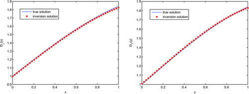
Inversion for $D_L(x)=1+x$ and $D_T(y)=1+y$

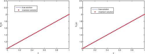
Considering $D_L(x)$ and $D_T(y)$ are both polynomial function, we choose $S=3$ and $Z=3$ for the truncation level and the exact solution of the inverse problem in this example is $R^{\mathit{true}}=(1,1,0,1,1,0)$. On the concrete computations in this example, we will chose the initial iteration as zero, i.e. $R^0=(0,0,0,0,0,0)$, CPU(s) denote the computational time for the numerical inversion and the other parameters are the same as Example 1.

According to the analysis of Example 1, here we will investigate two factors having influence on the inversion algorithm, which are the additional data and the numerical differential step, respectively. Choosing some points on four lines $(x_l,y)$ for $x_l=l/5(l=1,2,3,4)$ as the measured points, and noting $N_y=10$ in the computing of the forward problem, so the real measured points are chosen as $x_l,y_m$ for $x_l=l/5(l=1,2,3,4)$ and $y_m=m/10,m=0,1,\dots ,10$. For convenience of writing in the following statement, we denote $[u(x_l,y_m)]$ where $l=1,2,3,4$ and $m=0,1,2,\dots ,10$ as $4\times 11$ -dimensional vector of the additional data along with the four lines, where $u(1/5,y_m)$ is a 11-dimensional vector of the additional data along the measured line of $x=1/5$, etc. The $u(x_l,y_m,1)$ denotes the additional information given at the final time $T=1$ and the inversion results with additional data and initial iteration are listed in Tables 10, 11, and the comparison of reconstruction solution and true solution of $D_L(x)$ and $D_T(y)$ with $c=0.01$ is listed in Figure 2.

Table 10. Influence of additional data on the algorithm in Example 4.2.

$u(x_l,y_m,1)$	Err1	Err2	j / CPU(s)
$[u(1/5,y_m)]$	0.0462	7.5510e–19	86/180.90
$[u(3/5,y_m)]$	0.0398	1.2613e–18	84/177.58
$[u(1/5,y_k),u(2/5,y_m)]$	0.0453	6.8727e–19	84/178.37
$[u(1/5,y_m),u(4/5,y_m)]$	0.0420	4.6115e–18	84/175.35
$[u(1/5,y_m),u(2/5,y_m),u(3/5,y_m)]$	4.6743e–4	1.0757e–17	84/168.83
$[u(2/5,y_m),u(3/5,y_m),u(4/5,y_m)]$	4.9915e–4	5.8536e–18	84/173.84
$[u(1/5,y_m),u(3/5,y_m),u(4/5,y_m)]$	5.4438e–4	1.3041e–17	83/166.25
$[u(1/5,y_m),u(2/5,y_m),u(3/5,y_m),u(4/5,y_m)]$	2.8769e–4	1.5900e–18	83/166.24

Table 11. Influence of differential step on the algorithm with $l=2,3,4$ in Example 4.1.

c	$R^{\mathit{inv}}$	Err1	Err2	j / CPU(s)
0.2	divergent
0.15	divergent
0.1	(1.00, 1.00, 0.00, 1.00, 1.00, 0.00)	4.9483e–6	3.9509e–15	100/203.61
0.05	(1.00, 1.00, 0.00, 1.00, 1.00, 0.00)	1.0159e–4	1.0667e–16	87/175.80
0.01	(1.00, 1.00, 0.00, 1.00, 1.00, 0.00)	4.9915e–4	5.8536e–18	84/173.84
0.001	(1.00, 1.00, 0.00, 1.00, 1.00, 0.00)	4.0846e–4	3.4381e–20	84/174.26
0.0001	(1.00, 1.00, 0.00, 1.00, 1.00, 0.00)	3.2985e–4	2.6798e–20	84/173.43
0.00001	(1.00, 1.00, 0.00, 1.00, 1.00, 0.00)	3.2051e–4	3.5247e–21	84/171.36

Figure 2. Reconstruction solution and true solution of $D_L(x)$ and $D_T(y)$ with $l=2,3,4$.

From Tables 10, 11 and Figure 2, it can be seen that the inversion solution perfectly concide with the exact solutions, however, the choice of the additional data are important to the realization of the inversion algorithm. If choosing the additional data along one and two lines, the inversion solution error could be relative a little larger than choosing more than two measured lines, and the more of the additional data, the less of the time cost and iteration numbers. Furthermore, the numerical differential step also has important impact on the inversion algorithm. If choosing the numerical differential step $c\ge 0.15$, the inversion could be failure and the solution error could be taken minimum with $\mathit{\tau }=0.1$, but not be suitable for any case. For example, Taking one or two measured data as the additional data, the inversion could be divergent if $\mathit{\tau }=0.1$ by our calculated.

Example 4.3:

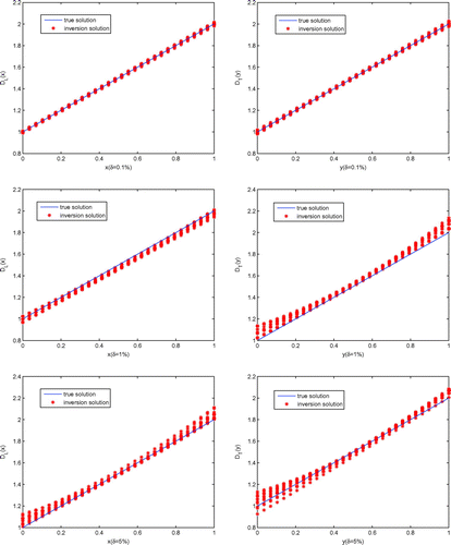
Inversion for $D_L(x)=exp(-x)$ and $D_T(y)=1+y$

We take $D_L(x)=e^{-x}$ and $D_T(y)=1+y$ in this example and $e^{-x}$ has the expansion$$e^{-x}=1-x+\frac{1}{2!}{x}^2-\frac{1}{3!}{x}^3+\cdots$$

Considering the truncation error for the expansion of $D_L(x)=e^{-x}$ by polynomial function, we choose $S=3,4,5$, $Z=3$ and $N=10$ and the parameters here are the same as the Examples 4.1 and 4.2 without regard to the cases of variable parameters. 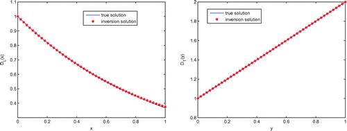Combing the analysis of Examples 4.1 and 4.2, the numerical inversion with respect to additional data, numerical differential step and the space dimension of ${\mathrm{\Phi }}_1$ which have influence on the inversion algorithm is given and the numerical results are listed in Tables 12–14, respectively. If taking the dimension of ${\mathrm{\Phi }}_1$ with $S=5$, the numerical differential step $c=0.01$ and the additional data $[u(1/5,y_m),u(2/5,y_m);u(3/5,y_m)]$, the comparison of exact solution and inversion solution is listed in Figure 3.

Table 12. Influence of additional data on the algorithm if $S=4$ in Example 4.3.

$u(x_l,y_m,1)$	Err1	Err2	j
$[u(1/5,y_m)]$	0.0310	2.2330e–15	73
$[u(3/5,y_m)]$	0.0260	4.4293e–15	71
$[u(1/5,y_k),u(2/5,y_m)]$	0.0278	4.8456e–15	71
$[u(3/5,y_m),u(4/5,y_m)]$	0.0279	3.6465e–15	71
$[u(1/5,y_m),u(2/5,y_m),u(3/5,y_m)]$	0.0063	8.3948e–15	70
$[u(2/5,y_m),u(3/5,y_m),u(4/5,y_m)]$	0.0063	4.8384e–15	70
$[u(1/5,y_m),u(3/5,y_m),u(4/5,y_m)]$	0.0063	8.4821e–15	70
$[u(1/5,y_m),u(2/5,y_m),u(3/5,y_m),u(4/5,y_m)]$	0.0063	1.3457e–14	69

Table 13. Influence of differential step on the algorithm with $l=1,2,3$ in Example 4.3.

c	$R^{\mathit{inv}}$	Err1	Err2	j
0.06	divergent
0.05	(1.00, –1.00, 0.50, 1.67, 1.00, 1.00, 0.00)	0.0063	9.1415e–14	157
0.01	(1.00, –1.00, 0.50, 1.67, 1.00, 1.00, 0.00)	0.0063	8.3948e–15	70
0.001	(1.00, –1.00, 0.50, 1.67, 1.00, 1.00, 0.00)	0.0063	9.9096e–18	69
0.0001	(1.00, –1.00, 0.50, 1.67, 1.00, 1.00, 0.00)	0.0063	9.0896e–18	69
0.00001	(1.00, –1.00, 0.50, 1.67, 1.00, 1.00, 0.00)	0.0063	1.1129e–18	69

Table 14. Influence of space dimension on the inversion with $l=1,2,3$ in Example 4.3.

S	$R^{\mathit{inv}}$	Err1	Err2	j
3	(0.98, –0.98, 0.49, 1.01, 1.01, 0.00)	0.0308	1.4091e–12	60
4	(1.00, –1.00, 0.50, 1.67, 1.00, 1.00, 0.00)	0.0063	8.3948e–15	70
5	( 1.00, –1.00, 0.50, –0.17, 0.04, 1.00, 1.00, 0.00)	0.0012	3.1386e–15	71

Figure 3. Reconstruction solution and true solution of $D_L(x)$ and $D_T(y)$ in Example 4.3.

From Tables 12–14 and Figure 3, we can see that the inversion solution perfectly consistent with the exact solutions as the same with Example 4.2. The additional data have important influence to the numerical inversion and the more the additional data, the small the inversion solution error. In addition, the numerical differential step seems have little impact on inversion algorithm in this example.

Example 4.4:

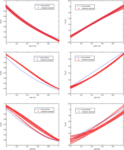
Inversion for $D_L(x)=exp(-x)$ and $D_T(y)=exp(-y)$

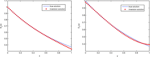
Similar to Example 4.3, we will give the numerical inversion with respect to additional data, numerical differential step and the space dimension of ${\mathrm{\Phi }}_1$ and ${\mathrm{\Phi }}_2$ which have influence on the inversion algorithm, the numerical results are listed in Tables 15–17, respectively. If taking the dimension $S=Z=5$, the numerical differential step $c=0.01$ and the additional data $[u(1/5,y_m),u(2/5,y_m);u(3/5,y_m)]$, the comparison of exact solution and inversion solution is listed in Figure 4.

Table 15. Influence of additional data on the algorithm if $S=Z=4$ in Example 4.4.

$u(x_l,y_m,1)$	Err1	Err2	j
$[u(1/5,y_m)]$	0.2467	1.8356e–13	63
$[u(4/5,y_m)]$	0.2752	3.6412e–14	59
$[u(1/5,y_k),u(2/5,y_m)]$	0.0857	1.6430e–14	62
$[u(3/5,y_m),u(4/5,y_m)]$	0.1187	6.6038e–14	61
$[u(1/5,y_m),u(2/5,y_m),u(3/5,y_m)]$	0.0194	8.2816e–14	59
$[u(2/5,y_m),u(3/5,y_m),u(4/5,y_m)]$	0.0334	4.8473e–14	60
$[u(1/5,y_m),u(2/5,y_m),u(3/5,y_m),u(4/5,y_m)]$	0.0207	4.2021e–14	59

Table 16. Influence of differential step on the algorithm with $l=1,2,3$ in Example 4.4.

c	$R^{\mathit{inv}}$	Err1	Err2	j
0.06	divergent
0.05	(1.00, –1.00, 0.50, –0.17, 0.96, –0.3507, –0.18, 0.29)	0.0212	6.5478e–13	230
0.01	( 1.00, –1.00, 0.50, –0.17, 0.96, –0.70, –0.18, 0.29)	0.0194	8.2816e–14	59
0.00001	(1.00, –1.00, 0.50, –0.17, 0.96, –0.70, –0.17, 0.29)	0.0212	1.8796e–17	69

Table 17. Influence of space dimension on the inversion with $l=1,2,3$ in Example 4.4.

S	$R^{\mathit{inv}}$	Err1	Err2	j
3	(0.75, –0.75, 0.37, 1.28, –1.28, 0.64)	0.2890	4.4896e–11	90
4	( 1.00, –1.00, 0.50, –0.17, 0.98, –0.79, –0.10, 0.30)	0.0194	8.2816e–14	59
5	(1.0, –1.0, 0.5, –0.17, 0.01, 0.98, –0.77, –0.18, 0.18, 0.18)	0.0120	2.3626e–14	62

Figure 4. Reconstruction solution and true solution of $D_L(x)$ and $D_T(y)$ in Example 4.4.

It could be seen from Tables 15–17 that the inversion solution error becomes small with the additional data increasing. However, the inversion solution error with three lines additional data $[u(1/5,y_m),u(2/5,y_m);u(3/5,y_m)]$ in Table 15 seems smaller than four lines, the numerical inversion result $R^{\mathit{inv}}=(1.0,-1.0,0.5,-0.16667,1.0,-1.0,0.5,-0.16667)$ with four lines is close to the expansion coefficient $R^{\mathit{true}}=(1,-1,1/2,-1/6,1,-1,1/2,-1/6)$. The space dimension has more important influence in this example, the inversion solution error will become large if taking lower space dimension and not hard to find that there is always some deviation with exact expansion coefficient for the inversion $D_T(y)$. In addition, the numerical differential step also have little impact on inversion algorithm here. From Figure 3, we can see that the inversion solution is well consistent with the exact solutions.

Example 4.5:

Inversion for $D_L(x)=1+\text{sin}(x)$ and $D_T(y)=1+\text{sin}(y)$

In this example, we will consider the diffusion coefficient with trigonometric function $D_L(x)=1+\text{sin}(x)$ and $D_T(y)=1+\text{sin}(y)$, where $1+\text{sin}(t)$ has the expansion$$1+\text{sin}(t)=1+t-\frac{1}{3!}{t}^3+\frac{1}{5!}{t}^5+\cdots$$

The numerical results with the impacts of the inversion solution with respect to the additional data and the space dimension are listed in Tables 18 and 19.

Table 18. Influence of additional data on the algorithm if $S=Z=4$ in Example 4.5.

$u(x_l,y_m,1)$	Err1	Err2	j
$[u(1/5,y_m)]$	0.0834	1.2024e–21	90
$[u(4/5,y_m)]$	0.0832	5.4857e–19	90
$[u(1/5,y_k),u(2/5,y_m)]$	0.0766	1.4325e–21	88
$[u(3/5,y_m),u(4/5,y_m)]$	0.0552	2.6386e–20	87
$[u(1/5,y_m),u(2/5,y_m),u(3/5,y_m)]$	0.0055	2.6687e–20	87
$[u(2/5,y_m),u(3/5,y_m),u(4/5,y_m)]$	0.0080	7.2819e–21	87
$[u(1/5,y_m),u(2/5,y_m),u(3/5,y_m),u(4/5,y_m)]$	0.0021	1.3921e–20	87

Table 19. Influence of space dimension on the inversion with $l=1,2,3$ in Example 4.5.

S	$R^{\mathit{inv}}$	Err1	Err2	j
3	(1.00, 1.00, 0.00, 1.00, 1.00, 0.00)	0.0463	5.5228e–20	87
4	(1.00, 1.00, 0.00, –0.17, 1.01, 0.97, 0.10, –0.25)	0.0055	2.6687e–20	87
5	( 0.97, 0.97, 0.01, –0.17, 0.01, 1.05, 0.88, 0.12, 0.68, –1.06)	0.0383	1.1189e–14	87

Figure 5. Reconstruction solution and true solution of $D_L(x)$ and $D_T(y)$ in Example 4.5.

Figure 6. The exact and ten-time inversion diffusion coefficients in Example 4.2.

Figure 7. The exact and ten-time inversion diffusion coefficients in Example 4.3.

From Tables 18, 19 and Figure 5, we can see that the inversion solution perfectly consistent with the exact solutions and the more the additional data, the small the inversion solution and iteration times. However, if taking space dimension $S=Z=5$, its inversion solution error is large than $S=Z=4$ which is different from the above examples and the deviation with exact expansion coefficient for the inversion $D_T(y)$ is still exist.

5. Numerical inversion with noisy data

In this section, we will perform the variable diffusion coefficients inversion in the case of noisy data to testify the numerical stability of the algorithm and the observation data with the noisy has the form as follows$$U_{\mathit{obs}}^{\mathit{noisy}}(\mathit{\delta })=(1+\mathit{\delta }\mathit{\xi })U_{\mathit{obs}}^{\mathit{LM}}$$

where $\mathit{\delta }>0$ is a noise level and $\mathit{\xi }$ is a random noise uniformly distributed in $[-1,1]$. According the discussion in Subsection 4.2, Three measured lines will be as the additional data and the other parameters here are the same as the above section except $c=0.01$, but we will perform the algorithm with continuous 10-times, where $\overline{R^{\mathit{inv}}}$ is the inversion solution of the ten-time inversions, $\overline{Err1}$ is the average relative inversion solution error and $\overline{j}$ is the average number of the iterations. The computational reconstruction solution with noisy data are listed in Tables 20, 21 and Figures 6, 7, respectively.

Table 20. The average inversion result with noisy data in Example 4.2.

$\mathit{\delta }$	$\overline{R^{\mathit{inv}}}$	$\overline{Err1}$	$\overline{j}$
0	(1.00, 1.00, 0.00, 1.00, 1.00, 0.00)	4.9915e–4	84
0.1%	(0.99, 1.00, –0.01, 1.01, 1.00, –0.01)	4.9603e–3	85
1%	(0.99, 0.94, 0.05, 1.03, 0.91, 0.10)	0.0246	78
5%	(1.07, 0.64, 0.34, 1.06, 0.72, 0.29)	0.0972	78.1

Table 21. The average inversion result with noisy data in Example 4.3.

$\mathit{\delta }$	$\overline{R^{\mathit{inv}}}$	$\overline{Err1}$	$\overline{j}$
0	(1.00, –1.00, 0.50, 1.67, 1.00, 1.00, 0.00)	0.0063	70
0.1%	(0.96, –0.98, 0.52, –0.1837, 1.01, 1.09, –0.08)	0.0215	58
1%	(1.05, –0.67, –0.26, 0.27, 0.99, 0.60, 0.36)	0.0643	52
5%	(1.09, –0.53, –0.41, 0.36, 1.05, 0.62, 0.41)	0.1217	52

From Tables 20, 21, and Figures 6, 7, we can see that the inversion algorithm is numerically stability when the additional data having the noisy data, and we also find that the iteration number will decrease with the noisy increasing and numerical inversion for $D_T(y)$ with noisy is also relatively not as good as $D_L(x)$.

6. Conclusions

We give three concluding remarks in this section.

(1)	The homotopy regularization algorithm is applied to solve the inverse problem of determining the space-dependent diffusion coefficients in the 2D space fractional diffusion equations. Such inversion algorithm is efficient for the inversion problem here, and it can be generalized to other simultaneous inversion problems in the multidimensional fractional diffusion equations. From the viewpoint of numerical inversion, the problem left is to deal with inverse problems of determining the discontinuous diffusion coefficients or some continuous diffusion coefficients but with high oscillations.
(2)	As we know it is still a difficult problem for solving the forward problem of multidimensional space fractional diffusion equations. The mesh steps not only have important influences on the accuracy of the numerical solutions, but also have great impacts on the computation time. In our numerical inversions, the computational time with $N_x=N_y$ and $N=80$ in Example 4.2 is about 170 s for one calculation, and similarly it becomes ten in Example 5.1, and it could become more than 1700 s. Thus, if we calculate twenty and more than twenty times or the mesh step becomes much smaller, the computational time increases much more. So the fast ADI differential scheme which keeps the accuracy and decreases computational complexity for the forward problem is very relevant.
(3)	The choice of additional data is of great importance to realization of the inversion algorithm especially for inverse problems in multidimensional cases. There are plenty of lines which can be chosen as the measured lines to get the additional data. The number of the additional data cannot be too few, otherwise the inversion could be failure. We will focus our attention on construction of effective schemes for the forward problem in high-dimensional case and utilization of suitable basis functions for the unknown in the sequent work.

Additional information

Funding

This work is supported by the National Natural Science Foundation of China [grant number 11371231].

Notes

No potential conflict of interest was reported by the authors.

This article was originally published with errors. This version has been corrected. Please see Erratum (https://doi.org/10.1080/17415977.2017.1414352). .

References

- Scher H, Montroll EW. Anomalous transit-time dispersion in amorphous solids. Phys Rev B. 1975;12:2455–2477.
- Benson DA. 1998. The fractional advection-dispersion equation: development and application. Dissertation of doctorial degree, University of Nevada, Reno, USA.
- Benson DA, Wheatcraft SW, Meerschaert MM. The fractional-order governing equation of levy motion. Water Resour Res. 2000;36:1413–1423.
- Dentz M, Cortis A, Scher H, Berkowitz H. Time behavior of solute transport in heterogeneous media: transition from anomalous to normal transport. Adv Water Res. 2004;27:55–173.
- Mainardi F. Fractional calculus and waves in linear viscoelasticity: an introduction to mathematical models. London: Imperial College Press; 2010.
- Zhou L, Selim HM. Application of the fractional advection-dispersion equations in porous media. Soil Sci Soc Am J. 2003;67:1079–1084.
- Schumer R, Benson DA, Meerschaert MM, et al. Euler derivation of the fractional advection dispersion equation. J Contam Hydrol. 2001;38:69–88.
- Kilbas AA, Srivastava HM, Trujillo JJ. Theory and applications of fractional differential equations. Amsterdam: Elsevier; 2006.
- Podlubny I. Fractional differential equations. San Diego: Academic; 1999.
- Bhrawy AH. A Jacobi spectral collocation method for solving multi-dimensional nonlinear fractional sub-diffusion equations. Numer Algorithms. 2016;73:91–113. DOI:10.1007/s11075-015-0087-2
- Bhrawy AH. A highly accurate collocation algorithm for 1+1 and 2+1 fractional percolation equations. J Vibr Cont. 2016;22:2288–2310.
- Bhrawy AH, Alofi AS. The operational matrix of fractional integration for shifted Chebyshev polynomials. Appl Math Lett. 2013;26:25–31.
- Saadatmandi A, Dehghan M. A new operational matrix for solving fractional-order differential equations. Comput Math Appl. 2010;59:1326–1336.
- Bhrawy AH, Taha TM, Machado JAT. A review of operational matrices and spectral techniques for fractional calculus. Nonlinear Dyn. 2015;81:1023–1052.
- Dehghan M, Abbaszadeh M. Analysis of the element free Galerkin (EFG) method for solving fractional cable equation with Dirichlet boundary condition. Appl Numer Math. 2016;109:208–234.
- Pang G, Chen W, Fu Z. Space-fractional advection-dispersion equations by the Kansa method. J Comput Phys. 2015;293:280–296.
- Fu ZJ, Chen W, Yang HT. Boundary particle method for Laplace transformed time fractional diffusion equations. J Comput Phys. 2013;235:52–66.
- Chen W, Pang G. A new definition of fractional Laplacian with application to modeling three-dimensional nonlocal heat conduction. J Comput Phys. 2016;309:350–367.
- Chen S, Liu F, Anh V. A novel implicit finite difference method for the one-dimensional fractional percolation. Numer Algorithms. 2011;56:517–535.
- Liu F, Zhuang P, Anh A, et al. Stability and convergence of the difference methods for the space-time fractional advection-diffusion equation. Appl Math Comput. 2007;191:12–20.
- Meerschaert MM, Tadjeran C. Finite difference approximations for fractional advection-dispersion flow equations. J Comput Appl Math. 2004;172:65–77.
- Gu Y, Gao H, Chen W, et al. Fast-multipole accelerated singular boundary method for large-scale three-dimensional potential problems. Int J Heat Mass Trans. 2015;90:291–301.
- Chen W, Gu Y. An improved formulation of singular boundary method. Adv Appl Math Mech. 2012;4:543–558.
- Meerschaert MM, Scheffler HP, Tadjeran C. Finite difference methods for two-dimensional fractional dispersion equation. J Comput Phys. 2006;211:249–261.
- Chen S, Liu F, Turner I, et al. An implicit numerical method for the two-dimensional fractional percolation equation. J Appl Math Comput. 2013;219:4322–4331.
- Wang H, Wang K. An O(NLog2N) alternating-direction finite difference method for two-dimensional fractional diffusion equation. Comput Phys. 2011;21:7830–7839.
- Li LM, Xu D. Alternating-direction implicit-eluer method for the two-dimensional fractional evolution equation. J Comput Phys. 2013;236:157–168.
- Bhrawy AH, Baleanu D. A spectral Legendre-Gauss-Lobatto collocation method for a space-fractional advection diffusion equations with variable coefficients. Rep Math Phys. 2013;72(2):219–233.
- Doha EH, Bhrawy AH, Ezz-Eldien SS. Numerical approximations for fractional diffusion equations via a Chebyshev spectral-tau method. Centr Europ J Phys. 2013;11(10):1494–1503.
- Huang Y, Zheng M. Pseudo-spectral method for space fractional diffusion equation. Appl Math. 2013;04(11):1495–1502.
- Li XJ, Xu CJ. Existence and uniqueness of the weak solution of the space-time fractional diffusion equation and a spectral method approximation. Commun Comput Phys. 2010;8(5):1016–1051.
- Li XJ, Xu CJ. A space-time spectral method for the time fractional diffusion equation. J Numer Anal. 2009;47(3):2108–2131.
- Bueno-Orovio A, Kay D, Burrage K. Fourier spectral methods for fractional-in-space reaction-diffusion equations. Bit Numer Math. 2014;54(4):937–954.
- Xu X, Cheng J, Yamamoto M. Carleman estimate for a fractional diffusion equation with half order and application. Appl Anal. 2011;90:1355–1371.
- Sakamoto K, Yamamoto M. Initial value/boundary value problems for fractional diffusion-wave equations and applications to some inverse problems. J Math Anal Appl. 2011;382:426–447.
- Yamamoto M, Zhang Y. Conditional stability in determining a zeroth-order coefficient in a half-order fractional diffusion equation by a Carleman estimate. Inverse Probl. 2012;28:105010.
- Jin BT, Rundell W. An inverse problem for a one-dimensional time-fractional diffusion problem. Inverse Probl. 2012;28:075010
- Tian WY, Li C, Deng WH, et al. Regularization methods for unknown source in space fractional diffusion equation. Math Comput Sim. 2012;85:45–56.
- Tuan VK. Inverse problem for fractional diffusion equation. Fract Calc Appl Anal. 2011;14:31–55.
- Xiong XT, Zhou Q, Hon YC. An inverse problem for fractional diffusion equation in 2-dimensional case: stability analysis and regularization. J Math Anal Appl. 2012;393:185–199.
- Zheng GH, Wei T. Two regularization methods for solving a Riesz-Feller space-fractional backward diffusion equation. Inverse Probl. 2010;26:115017.
- Chi GS, Li GS, Jia XZ. Numerical inversions of a source term in the FADE with Dirichlet boundary condition using final ovservations. Comput Math Appl. 2011;62:1619–1626.
- Wei H, Chen W, Sun HG, et al. A coupled method for inverse source problem of spatial fractional anomalous diffusion equations. Inverse Probl Sci Eng. 2010;18:945–956.
- Zhang DL, Lou HZ, Li GS, et al. Simultaneous inversion for dispersion coefficients and space-dependent source magnitude in 2D Transportation. J Math Res. 2013;5:65–78.
- Cheng J, Nakagawa J, Yamamoto M, et al. Uniqueness in an inverse problem for a one-dimensional fractional diffusion equation. Inverse Probl. 2009;25:115002.
- Li GS, Zhang DL, Jia XZ, et al. Simultaneous inversion for the space-dependent diffusion coefficient and the fractional order in the time-factional diffusion equation. Inverse Probl. 2013;29:065014.
- Li GS, Gu WJ, Jia XZ. Numerical inversions for space-dependent diffusion coefficient in the time fractional diffusion equation. J Inverse Ill Posed P. 2012;20:339–366.
- Bhrawy Ah, Abdelkawy MA. Efficient spectral collocation algorithm for solving parabolic inverse problems. Int J Comput Meth. 2016;13:1650036. DOI:10.1142/S02198762
- Shakeri F, Dehghan M. Inverse problem of diffusion equation by He’s homotopy perturbation method. Phys Scr. 2007;75:551–556.
- Dehghan M, Saadatmandi A. A tau method for the one-dimensional parabolic inverse problem subject to temperature overspecification. Comput Math Appl. 2006;52:933–940.
- Chi GS, Li GS. Numerical inversions for a nonlinear source term in the heat equation by optimal perturbation algorithm. Comput Math Appl. 2010;216:2408–2416.
- Gu Y, Chen W, Fu ZJ. Singular boundary method for inverse heat conduction problems in general anisotropic media. Inverse Probl Sci Eng. 2013;22:889–909.
- Gu Y, Chen W, Zhang C, et al. A meshless singular boundary method for three-dimensional inverse heat conduction problems in general anisotropic media. Int J Heat Mass Trans. 2015;84:91–102.
- Han B, Li L. Solving methods and applications for nonlinear improper problems. Beijing: Science Press; 2011.
- Ruan ZS, Xu DH, Wang ZW. Convergence on modified regularization method for a backwardin-time problem (in Chinese). Numer Math: A J Chinese U. 2011;33:156–168.
- Meerschaert MM, Tadjeran C. Finite difference approximations for fractional advection-dispersion flow equation. J Comput Appl Math. 2004;172:65–77.
- Li GS, Cheng J, Yao D, et al. One-dimensional equilibrium model and source parameter determination for soil-column experiment. Appl Math Comput. 2007;190:1365–1374.
- Li GS, Tan YJ, Yao D, et al. A nonlinear mathematical model for an undisturbed soil-column experiment and source parameter identification. Inverse Probl Sci Eng. 2008;16:885–901.
- Su CW. Numerical method and application of inverse problems in PDE. Xi’an: Northwestern Ploytechnical University Press; (in chinese).