Landweber iteration regularization method for identifying unknown source on a columnar symmetric domain

Abstract

In this paper, an inverse source problem for the Helium Production–Diffusion Equation on a columnar symmetric domain is investigated. Based on an a priori assumption, the optimal error bound analysis and a conditional stability result are given. This problem is ill-posed and Landweber iteration regularization method is used to deal with this problem. Convergence estimates are presented under the priori and the posteriori regularization choice rules. For the a priori and the a posteriori regularization parameters choice rules, the convergence error estimates are all order optimal. Numerical examples are given to show that the regularization method is effective and stable for dealing with this ill-posed problem.

Keywords:

• Inverse problem
• identifying the unknown source
• ill-posed problem
• regularization method
• columnar symmetric domain

AMS Subject Classifications:

• 35R25
• 47A52
• 35R30

1. Introduction

Source identification problem is the most commonly encountered inverse problems in heat conduction. These problems have been studied over several decades due to their significance in a variety of scientific and engineering applications such as in groundwater migration, pollution source identification and control, environmental protection [1].

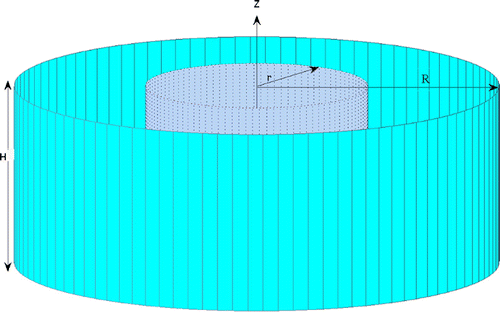
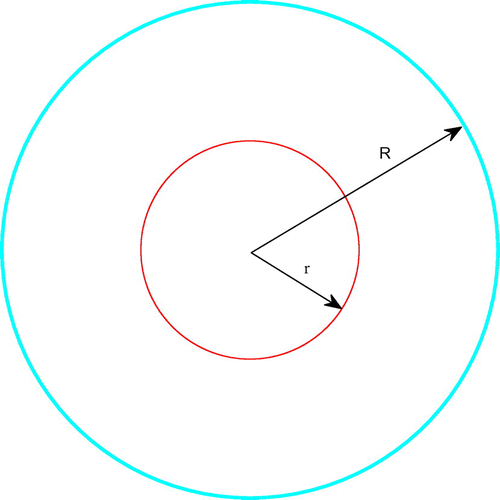
In this paper, we study the following source identification problem for the Helium production–diffusion equation [2] which considers the local helium concentration gradients resulting from ejection of high energy alpha particles from grain surfaces. It is assumed that the grain is of a columnar diffusion geometry as illustrated in Figures 1 and 2, which is actually consistent with laboratory measurements of helium diffusion

Figure 1. The 3-D model for the columnar symmetric domain.

Figure 2. The 2-D model for the columnar symmetric domain.

from apatite. As a consequence of radiogenic production and diffusive loss u(r, t) which only depends on the columnar symmetric domain radius r denotes the concentration of helium. We consider the following problem:(1.1) $$\begin{array}{c}\hfill \left\{\begin{array}{cc}{u}_t-\frac{1}{r}{u}_r-u_{rr}=f(r),\hfill & 0<t<T,0<r<r_0,\hfill \\ u(r,0)=0,\hfill & 0\le r\le r_0,\hfill \\ u(r_0,t)=0,\hfill & 0\le t\le T,\hfill \\ \underset{r\to 0}{lim}u(r,t)\text{is bounded}\hfill & 0<t<T,0<r<r_0.\hfill \end{array}\right.\end{array}$$(1.1)

The data are given as the final observation of the helium concentration:(1.2) $$\begin{array}{c}\hfill u(r,T)=g(r),0\le r\le r_0.\end{array}$$(1.2)

Given the data function g(r), the inverse radiogenic source problem is to reconstruct the source term f(r), which accounts for the ejection of high energy alpha particles. This problem is closely connected to the $(U-Th)/He$ isotopes dating, one method of low temperature thermochronometry. Since the $(U-Th)/He$ isotopes dating achieves a relative low temperature condition that cannot be reached by other isotopes systems, as well as the fact that high-precision, high-sensitivity Helium analysis are comparatively easy, it has been widely used in the study of mountain uplift and the geomorphic evolution, and the dating of terrestrial and extraterrestrial materials. For more physical context and applications, we refer to the papers [2–4] and the references cited therein. Since the data g(r) are based on (physical) observation, there must be measurement error, and we assume the measured data function $g^{\mathit{\delta }}(r)$ satisfies(1.3) $$\begin{array}{c}\hfill \Vert g^{\mathit{\delta }}(·)-g(·)\Vert \le \mathit{\delta }.\end{array}$$(1.3)

Besides the motivation of the radiogenic source identification for the helium diffusion, heat source identification problem is an important branch in inverse problem research. About source identification problem, due to their significance in a variety of scientific and engineering application, it has been studied over several decades. Now about various types of heat sources in one dimensional, there are much research results, such as [5–32]. Compared with one-dimensional diffusion equation, about the high-dimensional case, there is relative little research result. In [33], the authors took the Landweber iteration as a numerical method to identify unknown source in columnar domain. In [34], the authors also took the Landweber iteration as a numerical method to identify spatial source in a bound domain. But in [33,34], the authors cannot give the error estimate between the exact solution and the regularization solution. In [35], the authors used the spectral method to identify the heat source in a spherically symmetric parabolic equation. In [36], the authors used the spectral method to identify the heat source in columnar symmetric domain and proved the uniqueness of a solution. But in [35,36], the regularization parameters are selected by the a priori rule. There is a defect for any a priori method, i.e. the a priori choice of the regularization parameter depends seriously on the a priori bound E of the unknown solution. However, the a priori bound E cannot be known exactly in practice, and working with a wrong constant E may lead to the bad regularized solution. Moreover the error estimates in [35,36] are only logarithm type.

In this study, one of our purposes is that Landweber iteration as a regularization method is firstly used to deal with this problem. Secondly, we prove an optimal error bound of this problem is Hölder type under a special ‘source condition’. The third purpose is that we give the a priori and a posteriori choice of the regularization parameters for Landweber iteration regularization method. For a priori and a posteriori choices of the regularization parameter, we all obtain the Hölder type stability estimates which are all order optimal. Finally, we give some different examples to show the comparison of numerical effect between a priori and a posteriori regularization choice rules.

Throughout this paper, $L^2[0,r_0;r]$ denotes the Hilbert space of Lebesgue measurable functions f with weight r on $[0,r_0]$. $(·,·)$ and $\Vert ·\Vert$ denote the inner and norm on $L^2[0,r_0;r]$, respectively, with the norm(1.4) $$\begin{array}{c}\hfill \Vert f(·)\Vert ={\left({\int }_0^{r_0}r{|f(r)|}^2\mathrm{d}r\right)}^{\frac{1}{2}}.\end{array}$$(1.4)

Using the method of separation of variable, we get the solution of problem (1.1(1.1) $$\begin{array}{c}\hfill \left\{\begin{array}{cc}{u}_t-\frac{1}{r}{u}_r-u_{rr}=f(r),\hfill & 0<t<T,0<r<r_0,\hfill \\ u(r,0)=0,\hfill & 0\le r\le r_0,\hfill \\ u(r_0,t)=0,\hfill & 0\le t\le T,\hfill \\ \underset{r\to 0}{lim}u(r,t)\text{is bounded}\hfill & 0<t<T,0<r<r_0.\hfill \end{array}\right.\end{array}$$(1.1) )(see [36]):(1.5) $$\begin{array}{c}\hfill u(r,t)=\sum _{n=1}^{\infty }\left(f(·),X_n(·)\right)k_n(t)X_n(r),\end{array}$$(1.5)

where(1.6) $$\begin{array}{c}\hfill k_n(t)={\left(\frac{r_0}{u_n}\right)}^2\left(1-e^{-{\left(\frac{u_n}{r_0}\right)}^{2}t}\right),X_n(r)=\frac{\sqrt{2}}{r_0{J}_1(u_n)}{J}_0\left(\frac{u_{n}r}{r_0}\right),n=1,2,3,\dots ,\end{array}$$(1.6)

and $\{X_n(r)\}$ is an orthonormal basis of $L^2[0,r_0;r]$, $J_0(.)$ and $J_1(.)$ is Zero-order Bessel function and First-order Bessel function, respectively. $u_n$ is the infinite number real roots of the equation(1.7) $$\begin{array}{c}\hfill J_0(r)=0,\end{array}$$(1.7)

and satisfies(1.8) $$\begin{array}{c}\hfill 0<u_1<u_2<u_3<···<u_n<···,\underset{n\to \infty }{lim}{u}_n=\infty .\end{array}$$(1.8)

Denote(1.9) $$\begin{array}{c}\hfill f_n=(f(·),X_n(·))={\int }_0^{r_0}rf(r)X_n(r)\mathrm{d}r,g_n=(g(·),X_n(·))={\int }_0^{r_0}rg(r)X_n(r)\mathrm{d}r.\end{array}$$(1.9)

Throughout this paper, all scalar product is computed by (1.9(1.9) $$\begin{array}{c}\hfill f_n=(f(·),X_n(·))={\int }_0^{r_0}rf(r)X_n(r)\mathrm{d}r,g_n=(g(·),X_n(·))={\int }_0^{r_0}rg(r)X_n(r)\mathrm{d}r.\end{array}$$(1.9) ). Using $u(r,T)=g(r)$, we obtain(1.10) $$\begin{array}{c}\hfill g(r)=\sum _{n=1}^{\infty }{f}_n{k}_n{X}_n(r)\end{array}$$(1.10)

and(1.11) $$\begin{array}{c}\hfill f(r)=\sum _{n=1}^{\infty }\frac{g_n}{k_n}{X}_n(r),\end{array}$$(1.11)

where(1.12) $$\begin{array}{c}\hfill k_n=T{e}^{-{\left(\frac{u_n}{r_0}\right)}^2(T-t_n)}.\end{array}$$(1.12)

From Equation (1.11(1.11) $$\begin{array}{c}\hfill f(r)=\sum _{n=1}^{\infty }\frac{g_n}{k_n}{X}_n(r),\end{array}$$(1.11) ), we can see that $k_n^{-1}\to \infty$ as $n\to \infty$. So the exact data function g(r) must satisfy the property that $(g,X_n(·))$ decays rapidly. But in applications, the input data g(r) can only be measured and never be exact. As for the measured data function $g^{\mathit{\delta }}(r)$ only belongs to $L^2[0,r_0;r]$, we cannot expect it has the same decay rate in $L^2[0,r_0;r]$. Thus the problem (1.1(1.1) $$\begin{array}{c}\hfill \left\{\begin{array}{cc}{u}_t-\frac{1}{r}{u}_r-u_{rr}=f(r),\hfill & 0<t<T,0<r<r_0,\hfill \\ u(r,0)=0,\hfill & 0\le r\le r_0,\hfill \\ u(r_0,t)=0,\hfill & 0\le t\le T,\hfill \\ \underset{r\to 0}{lim}u(r,t)\text{is bounded}\hfill & 0<t<T,0<r<r_0.\hfill \end{array}\right.\end{array}$$(1.1) ) is ill-posed. So we must use regularization method to deal with problem (1.1(1.1) $$\begin{array}{c}\hfill \left\{\begin{array}{cc}{u}_t-\frac{1}{r}{u}_r-u_{rr}=f(r),\hfill & 0<t<T,0<r<r_0,\hfill \\ u(r,0)=0,\hfill & 0\le r\le r_0,\hfill \\ u(r_0,t)=0,\hfill & 0\le t\le T,\hfill \\ \underset{r\to 0}{lim}u(r,t)\text{is bounded}\hfill & 0<t<T,0<r<r_0.\hfill \end{array}\right.\end{array}$$(1.1) ). Before this, we still give an a priori bound on the unknown heat source.

Denote$$\begin{array}{c}\hfill Q_p=\left\{\mathit{\psi }\in L^2[0,r_0;r];\sum _{n=1}^{\infty }{\left(\frac{u_n}{r_0}\right)}^p{|(\mathit{\psi }(·),X_n(·))|}^2<\infty \right\},\end{array}$$

where $(·,·)$ is product of $L^2[0,r_0;r]$, $p>0$ is a constant, then $Q_p$ is a Hilbert space which norm is denoted by(1.13) $$\begin{array}{c}\hfill {\Vert \mathit{\psi }\Vert }_{Q_p}:={\left(\sum _{n=1}^{\infty }{\left(\frac{u_n}{r_0}\right)}^p{|(\mathit{\psi },X_n(·))|}^2\right)}^{\frac{1}{2}}.\end{array}$$(1.13)

So we suppose(1.14) $$\begin{array}{c}\hfill {\Vert f(·)\Vert }_{Q_p}\le E,\end{array}$$(1.14)

where $E>0$ is a constant.

This paper is organized as follows. Section 2 gives the optimal error bound for problem (1.1(1.1) $$\begin{array}{c}\hfill \left\{\begin{array}{cc}{u}_t-\frac{1}{r}{u}_r-u_{rr}=f(r),\hfill & 0<t<T,0<r<r_0,\hfill \\ u(r,0)=0,\hfill & 0\le r\le r_0,\hfill \\ u(r_0,t)=0,\hfill & 0\le t\le T,\hfill \\ \underset{r\to 0}{lim}u(r,t)\text{is bounded}\hfill & 0<t<T,0<r<r_0.\hfill \end{array}\right.\end{array}$$(1.1) ). Section 3 gives the conditional stability estimate for problem (1.1(1.1) $$\begin{array}{c}\hfill \left\{\begin{array}{cc}{u}_t-\frac{1}{r}{u}_r-u_{rr}=f(r),\hfill & 0<t<T,0<r<r_0,\hfill \\ u(r,0)=0,\hfill & 0\le r\le r_0,\hfill \\ u(r_0,t)=0,\hfill & 0\le t\le T,\hfill \\ \underset{r\to 0}{lim}u(r,t)\text{is bounded}\hfill & 0<t<T,0<r<r_0.\hfill \end{array}\right.\end{array}$$(1.1) ). Section 4 obtains the order-optimal error estimates under the a priori and the a posteriori parameter choice rules. Section 5 gives some numerical examples to show the effectiveness of this method. Section 6 puts an end to this paper with a brief conclusion.

2. Preliminary result and optimal error bound for problem (1.1(1.1) $$\begin{array}{c}\hfill \left\{\begin{array}{cc}{u}_t-\frac{1}{r}{u}_r-u_{rr}=f(r),\hfill & 0<t<T,0<r<r_0,\hfill \\ u(r,0)=0,\hfill & 0\le r\le r_0,\hfill \\ u(r_0,t)=0,\hfill & 0\le t\le T,\hfill \\ \underset{r\to 0}{lim}u(r,t)\text{is bounded}\hfill & 0<t<T,0<r<r_0.\hfill \end{array}\right.\end{array}$$(1.1) )

2.1. Preliminary result

To find f(r), we define a linear operator $K:L^2[0,r_0;r]\to L^2[0,r_0;r]$, and only need to solve the following integral equation:(2.1) $$\begin{array}{c}\hfill Kf(r)={\int }_0^{r_0}k(r,\mathit{\xi })f(\mathit{\xi })\mathrm{d}\mathit{\xi }=g(r),\end{array}$$(2.1)

where(2.2) $$\begin{array}{c}\hfill k(r,\mathit{\xi })=\sum _{n=1}^{\infty }{k}_n{X}_n(r)X_n(\mathit{\xi }).\end{array}$$(2.2)

From (2.2(2.2) $$\begin{array}{c}\hfill k(r,\mathit{\xi })=\sum _{n=1}^{\infty }{k}_n{X}_n(r)X_n(\mathit{\xi }).\end{array}$$(2.2) ), we know $k(r,\mathit{\xi })=k(\mathit{\xi },r)$, so K is a self-adjoint and compact operator. Now we give a important Lemma as follows:

Lemma 2.1:

[see in [37,38]] Let ${\{k_n\}}_{n=1}^{\infty }$ mention (1.12(1.12) $$\begin{array}{c}\hfill k_n=T{e}^{-{\left(\frac{u_n}{r_0}\right)}^2(T-t_n)}.\end{array}$$(1.12) ). Let $u_n$ be the infinite number real roots of the equation $J_0(r)=0$, so there exist two positive constants $C_1$ and $C_2$ such that(2.3) $$\begin{array}{c}\hfill \frac{C_1}{u_n}\le k_n\le \frac{C_2}{u_n}.\end{array}$$(2.3)

Consider an arbitrary ill-posed operator equation [40–44]:(2.4) $$\begin{array}{c}\hfill Ax=y,\end{array}$$(2.4)

where $A:L^2[0,r_0;r]\to L^2[0,r_0;r]$ is a linear bounded between infinite dimensional Hilbert spaces X and Y with non-closed range R(A) of A. Assume that $y^{\mathit{\delta }}\in Y$ are available noisy data with $\Vert y-y^{\mathit{\delta }}\Vert \le \mathit{\delta }$. Any operator $R:Y\to X$ can be considered as a special method for approximately solving (2.4(2.4) $$\begin{array}{c}\hfill Ax=y,\end{array}$$(2.4) ), and the approximate solution of (2.4(2.4) $$\begin{array}{c}\hfill Ax=y,\end{array}$$(2.4) ) is given by $R{y}^{\mathit{\delta }}$.

Let $M\subset X$ be a bounded set. Let us introduce the worst case error $▵(\mathit{\delta },R)$ for identifying x from $y^{\mathit{\delta }}$ as [39–43]:(2.5) $$\begin{array}{c}\hfill ▵(\mathit{\delta },R):=sup\left\{\Vert R{y}^{\mathit{\delta }}-x\Vert |x\in M,y^{\mathit{\delta }}\in Y,\Vert Ax-y^{\mathit{\delta }}\Vert \le \mathit{\delta }\right\}.\end{array}$$(2.5)

The best possible error bound (or optimal error bound) is defined as the infimum over all mappings $R:Y\to X$:(2.6) $$\begin{array}{c}\hfill \mathit{\omega }(\mathit{\delta }):=\underset{R}{inf}▵(\mathit{\delta },R).\end{array}$$(2.6)

Now let us review some optimality results if the set $M=M_{\mathit{\phi },E}$ is given by(2.7) $$\begin{array}{c}\hfill M_{\mathit{\phi },E}=\left\{x\in X|x={[\mathit{\phi }(A^{\ast }A)]}^{-\frac{1}{2}}v,\Vert v\Vert \le E\right\},\end{array}$$(2.7)

where the operator function $\mathit{\phi }(A^{\ast }A)$ is well defined via spectral representation [30,42,45](2.8) $$\begin{array}{c}\hfill \mathit{\phi }(A^{\ast }A)={\int }_0^a\mathit{\phi }(\mathit{\lambda })\mathrm{d}{E}_{\mathit{\lambda }},\end{array}$$(2.8)

where $A^{\ast }A={\int }_0^a\mathit{\lambda }d{E}_{\mathit{\lambda }}$ is the spectral decomposition of $A^{\ast }A$, $E_{\mathit{\lambda }}$ denotes the spectral family of the operator $A^{\ast }A$. a is a constant which satisfies $\Vert A^{\ast }A\Vert \le a$. In the case when A is a multiplication operator, $Ax(s)=\mathit{\gamma }(s)x(s)$, the operator function $\mathit{\phi }(A^{\ast }A)$ has the form(2.9) $$\begin{array}{c}\hfill \mathit{\phi }\left(A^{\ast }{A)x(s)=\mathit{\phi }(|\mathit{\gamma }(s)|}^2\right)x(s).\end{array}$$(2.9)

Then a method $R_0$ is called [43]

(i)	optimal on the set $M_{\mathit{\phi },E}$ if $▵(\mathit{\delta },R_0)=\mathit{\omega }(\mathit{\delta },E)$ holds;
(ii)	order optimal on the set $M_{\mathit{\phi },E}$ if $▵(\mathit{\delta },R_0)\le C\mathit{\omega }(\mathit{\delta },E)$ with $C\ge 1$ holds.

In order to derive an explicit (best possible) optimal error bound for the worst case error $▵(\mathit{\delta },R)$ defined in (2.5(2.5) $$\begin{array}{c}\hfill ▵(\mathit{\delta },R):=sup\left\{\Vert R{y}^{\mathit{\delta }}-x\Vert |x\in M,y^{\mathit{\delta }}\in Y,\Vert Ax-y^{\mathit{\delta }}\Vert \le \mathit{\delta }\right\}.\end{array}$$(2.5) ), we assume that the function $\mathit{\phi }$ in (2.8(2.8) $$\begin{array}{c}\hfill \mathit{\phi }(A^{\ast }A)={\int }_0^a\mathit{\phi }(\mathit{\lambda })\mathrm{d}{E}_{\mathit{\lambda }},\end{array}$$(2.8) 2.9(2.9) $$\begin{array}{c}\hfill \mathit{\phi }\left(A^{\ast }{A)x(s)=\mathit{\phi }(|\mathit{\gamma }(s)|}^2\right)x(s).\end{array}$$(2.9) ) satisfies the following assumption:

Assumption 2.1.1:

[42,43,45]] The function $\mathit{\phi }(\mathit{\lambda }):(0,a]\to (0,\infty )$ in (2.8(2.8) $$\begin{array}{c}\hfill \mathit{\phi }(A^{\ast }A)={\int }_0^a\mathit{\phi }(\mathit{\lambda })\mathrm{d}{E}_{\mathit{\lambda }},\end{array}$$(2.8) ), where a is a constant such that $\Vert A^{\ast }A\Vert \le a$, is continuous and has the following properties:

(i)	${lim}_{\mathit{\lambda }\to 0}\mathit{\phi }(\mathit{\lambda })=0$;
(ii)	$\mathit{\phi }$ is strictly monotonically increasing on (0, a];
(iii)	$\mathit{\rho }(\mathit{\lambda })=\mathit{\lambda }{\mathit{\phi }}^{-1}(\mathit{\lambda }):(0,\mathit{\phi }(a)]\to (0,a\mathit{\phi }(a)]$ is convex.

Now we will formulate our main result of this section concerning the best possible worst case error $\mathit{\omega }(\mathit{\delta },E)$ defined in (2.6(2.6) $$\begin{array}{c}\hfill \mathit{\omega }(\mathit{\delta }):=\underset{R}{inf}▵(\mathit{\delta },R).\end{array}$$(2.6) ) for identifying the solution f of problem (1.1(1.1) $$\begin{array}{c}\hfill \left\{\begin{array}{cc}{u}_t-\frac{1}{r}{u}_r-u_{rr}=f(r),\hfill & 0<t<T,0<r<r_0,\hfill \\ u(r,0)=0,\hfill & 0\le r\le r_0,\hfill \\ u(r_0,t)=0,\hfill & 0\le t\le T,\hfill \\ \underset{r\to 0}{lim}u(r,t)\text{is bounded}\hfill & 0<t<T,0<r<r_0.\hfill \end{array}\right.\end{array}$$(1.1) ) from noisy data $g^{\mathit{\delta }}$ under condition (1.3(1.3) $$\begin{array}{c}\hfill \Vert g^{\mathit{\delta }}(·)-g(·)\Vert \le \mathit{\delta }.\end{array}$$(1.3) ) and $f\in M_{\mathit{\phi },E}$, where the set $M_{\mathit{\phi },E}$ is given by (2.7(2.7) $$\begin{array}{c}\hfill M_{\mathit{\phi },E}=\left\{x\in X|x={[\mathit{\phi }(A^{\ast }A)]}^{-\frac{1}{2}}v,\Vert v\Vert \le E\right\},\end{array}$$(2.7) ). We introduce the optimal error bound by(2.10) $$\begin{array}{c}\hfill \mathit{\omega }(\mathit{\delta },E):=\underset{R}{inf}sup\{\Vert R{g}^{\mathit{\delta }}-f\Vert |f\in M_{\mathit{\phi },E},g^{\mathit{\delta }}\in L^2[0,r_0;r],\Vert g-g^{\mathit{\delta }}\Vert \le \mathit{\delta }\},\end{array}$$(2.10)

where R is an arbitrary method for approximation solving problem (1.1(1.1) $$\begin{array}{c}\hfill \left\{\begin{array}{cc}{u}_t-\frac{1}{r}{u}_r-u_{rr}=f(r),\hfill & 0<t<T,0<r<r_0,\hfill \\ u(r,0)=0,\hfill & 0\le r\le r_0,\hfill \\ u(r_0,t)=0,\hfill & 0\le t\le T,\hfill \\ \underset{r\to 0}{lim}u(r,t)\text{is bounded}\hfill & 0<t<T,0<r<r_0.\hfill \end{array}\right.\end{array}$$(1.1) ), $sup\{\Vert R{g}^{\mathit{\delta }}-f\Vert \}$ means the maximum error(the worst case error) between the $R{g}^{\mathit{\delta }}$ and f as $f\in M_{\mathit{\phi },E},g^{\mathit{\delta }}\in L^2[0,r_0;r],\Vert g-g^{\mathit{\delta }}\Vert \le \mathit{\delta }$, ${inf}_{R}sup\{\Vert R{g}^{\mathit{\delta }}-f\Vert \}$ means the smallest case error between the $R{g}^{\mathit{\delta }}$ and f for all mapping $R:Y\to M_{\mathit{\phi },E}$, which is called the optimal error bound.

Under Assumption 2.1.1, the next theorem gives us a general formula for the optimal error bound.

Theorem 2.1:

[42,43,45]] Let $M_{\mathit{\phi },E}$ be given by (2.7(2.7) $$\begin{array}{c}\hfill M_{\mathit{\phi },E}=\left\{x\in X|x={[\mathit{\phi }(A^{\ast }A)]}^{-\frac{1}{2}}v,\Vert v\Vert \le E\right\},\end{array}$$(2.7) ), let Assumption 2.1.1 be satisfied, and let $\frac{{\mathit{\delta }}^2}{E^2}\in \mathit{\sigma }(A^{\ast }A\mathit{\phi }(A^{\ast }A))$, where $\mathit{\sigma }(A^{\ast }A)$ denotes the spectrum of operator $A^{\ast }A$, then(2.11) $$\begin{array}{c}\hfill \mathit{\omega }(\mathit{\delta },E)=E\sqrt{{\mathit{\rho }}^{-1}\left(\frac{{\mathit{\delta }}^2}{E^2}\right)}.\end{array}$$(2.11)

2.2. Optimal error bound for problem (1.1(1.1) $$\begin{array}{c}\hfill \left\{\begin{array}{cc}{u}_t-\frac{1}{r}{u}_r-u_{rr}=f(r),\hfill & 0<t<T,0<r<r_0,\hfill \\ u(r,0)=0,\hfill & 0\le r\le r_0,\hfill \\ u(r_0,t)=0,\hfill & 0\le t\le T,\hfill \\ \underset{r\to 0}{lim}u(r,t)\text{is bounded}\hfill & 0<t<T,0<r<r_0.\hfill \end{array}\right.\end{array}$$(1.1) )

In this section, we consider the best possible worst case error (2.6(2.6) $$\begin{array}{c}\hfill \mathit{\omega }(\mathit{\delta }):=\underset{R}{inf}▵(\mathit{\delta },R).\end{array}$$(2.6) ) for identifying f(r) from noisy data $g^{\mathit{\delta }}(r)$ provided (1.3(1.3) $$\begin{array}{c}\hfill \Vert g^{\mathit{\delta }}(·)-g(·)\Vert \le \mathit{\delta }.\end{array}$$(1.3) ) and $f\in M_{p,E}$ hold, where $M_{p,E}$ is given by(2.12) $$\begin{array}{c}\hfill f\in M_{p,E}=\left\{f\in L^2[0,r_0;r]{|\Vert f\Vert }_{Q_p}\le E,p>0\right\},\end{array}$$(2.12)

where ${\Vert ·\Vert }_{Q_p}$ denotes the norm in Sobolev space $Q_p$ with(2.13) $$\begin{array}{c}\hfill {\Vert f(·)\Vert }_{Q_p}:={\left(\sum _{n=1}^{\infty }{\left(\frac{u_n}{r_0}\right)}^p{|(f(·),X_n(·))|}^2\right)}^{\frac{1}{2}}.\end{array}$$(2.13)

Let us formulate problem (1.1(1.1) $$\begin{array}{c}\hfill \left\{\begin{array}{cc}{u}_t-\frac{1}{r}{u}_r-u_{rr}=f(r),\hfill & 0<t<T,0<r<r_0,\hfill \\ u(r,0)=0,\hfill & 0\le r\le r_0,\hfill \\ u(r_0,t)=0,\hfill & 0\le t\le T,\hfill \\ \underset{r\to 0}{lim}u(r,t)\text{is bounded}\hfill & 0<t<T,0<r<r_0.\hfill \end{array}\right.\end{array}$$(1.1) ) as an operator equation(2.14) $$\begin{array}{c}\hfill Af=g\end{array}$$(2.14)

with linear operator $A\in \mathcal{L}(L^2[0,r_0;r],L^2[0,r_0;r])$. From (1.10(1.10) $$\begin{array}{c}\hfill g(r)=\sum _{n=1}^{\infty }{f}_n{k}_n{X}_n(r)\end{array}$$(1.10) ), we obtain(2.15) $$\begin{array}{c}\hfill \sum _{n=1}^{\infty }{\left(\frac{r_0}{u_n}\right)}^2\left(1-e^{-{\left(\frac{u_n}{r_0}\right)}^{2}T}\right)(f(·),X_n(·))X_n(r)=g(r).\end{array}$$(2.15)

So the singular values of operator A are(2.16) $$\begin{array}{c}\hfill {\mathit{\sigma }}_n={\left(\frac{r_0}{u_n}\right)}^2\left(1-e^{-{\left(\frac{u_n}{r_0}\right)}^{2}T}\right).\end{array}$$(2.16)

Proposition 2.2.1:

Consider the operator Equation (2.14(2.14) $$\begin{array}{c}\hfill Af=g\end{array}$$(2.14) ), the set $M_{p,E}$ is given in (2.12(2.12) $$\begin{array}{c}\hfill f\in M_{p,E}=\left\{f\in L^2[0,r_0;r]{|\Vert f\Vert }_{Q_p}\le E,p>0\right\},\end{array}$$(2.12) ). So $\mathit{\phi }=\mathit{\phi }(\mathit{\lambda })$ is given (in parameter representation) by(2.17) $$\begin{array}{c}\hfill \left\{\begin{array}{c}\mathit{\lambda }(l)={\left(\frac{1-e^{-l^{2}T}}{l^2}\right)}^2,\hfill \\ \mathit{\phi }(l)=l^{-p},\hfill \end{array}\right.0\le l<\infty .\end{array}$$(2.17)

Proof Comparing (2.13(2.13) $$\begin{array}{c}\hfill {\Vert f(·)\Vert }_{Q_p}:={\left(\sum _{n=1}^{\infty }{\left(\frac{u_n}{r_0}\right)}^p{|(f(·),X_n(·))|}^2\right)}^{\frac{1}{2}}.\end{array}$$(2.13) ) with (2.7(2.7) $$\begin{array}{c}\hfill M_{\mathit{\phi },E}=\left\{x\in X|x={[\mathit{\phi }(A^{\ast }A)]}^{-\frac{1}{2}}v,\Vert v\Vert \le E\right\},\end{array}$$(2.7) ), we obtain(2.18) $$\begin{array}{c}\hfill \mathit{\phi }(A^{\ast }A)={\left(\frac{u_n^2}{r_0^2}\right)}^{-p}.\end{array}$$(2.18)

Due to (1.11(1.11) $$\begin{array}{c}\hfill f(r)=\sum _{n=1}^{\infty }\frac{g_n}{k_n}{X}_n(r),\end{array}$$(1.11) ), we obtain that $\mathit{\phi }$ is given (in parameter representation) by $\mathit{\lambda }(u_n)={\left(\frac{r_0^2\left(1-e^{-{\left(\frac{u_n}{r_0}\right)}^{2}T}\right)}{u_n^2}\right)}^2$, $\mathit{\phi }(u_n)={\left(\frac{u_n^2}{r_0^2}\right)}^{-p}$. We substitute $\frac{u_n^2}{r_0^2}=l$ and obtain (2.17(2.17) $$\begin{array}{c}\hfill \left\{\begin{array}{c}\mathit{\lambda }(l)={\left(\frac{1-e^{-l^{2}T}}{l^2}\right)}^2,\hfill \\ \mathit{\phi }(l)=l^{-p},\hfill \end{array}\right.0\le l<\infty .\end{array}$$(2.17) )).

We will discuss properties of the function $\mathit{\phi }=\mathit{\phi }(\mathit{\lambda })(\mathit{\lambda }\in (0,\infty ))$ which is given (in parameter representation) by (2.17(2.17) $$\begin{array}{c}\hfill \left\{\begin{array}{c}\mathit{\lambda }(l)={\left(\frac{1-e^{-l^{2}T}}{l^2}\right)}^2,\hfill \\ \mathit{\phi }(l)=l^{-p},\hfill \end{array}\right.0\le l<\infty .\end{array}$$(2.17) ) in the following.

Proposition 2.2.2:

The function $\mathit{\phi }(\mathit{\lambda })$ defined by (2.17(2.17) $$\begin{array}{c}\hfill \left\{\begin{array}{c}\mathit{\lambda }(l)={\left(\frac{1-e^{-l^{2}T}}{l^2}\right)}^2,\hfill \\ \mathit{\phi }(l)=l^{-p},\hfill \end{array}\right.0\le l<\infty .\end{array}$$(2.17) ) is continuous and has the following properties:

(i)	${lim}_{\mathit{\lambda }\to 0}\mathit{\phi }(\mathit{\lambda })=0$.
(ii)	$\mathit{\phi }$ is strictly monotonically increasing.
(iii)	$\mathit{\rho }(\mathit{\lambda })=\mathit{\lambda }{\mathit{\phi }}^{-1}(\mathit{\lambda })$ is strictly monotonically increasing and possesses the following parameter representation: (2.19) $$\begin{array}{c}\hfill \left\{\begin{array}{c}\mathit{\lambda }(l)=l^{-p},\hfill \\ \mathit{\rho }(l)=l^{-p}{\left(\frac{1-e^{-l^{2}T}}{l^2}\right)}^2,\hfill \end{array}\right.0\le l<\infty .\end{array}$$(2.19)
(iv)	${\mathit{\rho }}^{-1}(\mathit{\lambda })$ is strictly monotonically increasing and possesses the following parameter representation: (2.20) $$\begin{array}{c}\hfill \left\{\begin{array}{c}\mathit{\lambda }(l)=l^{-p}{\left(\frac{1-e^{-l^{2}T}}{l^2}\right)}^2,\hfill \\ {\mathit{\rho }}^{-1}(l)=l^{-p},\hfill \end{array}\right.0\le l<\infty .\end{array}$$(2.20)
(v)	For the inverse function ${\mathit{\rho }}^{-1}(\mathit{\lambda })$, there holds (2.21) $$\begin{array}{c}\hfill {\mathit{\rho }}^{-1}(\mathit{\lambda })={\mathit{\lambda }}^{\frac{p}{p+2}}(1+o(1)),for\mathit{\lambda }\to 0.\end{array}$$(2.21)

Proof The proof of (i)–(iv) are obvious. We only give the proof of (v). Let $F(\mathit{\lambda })={\mathit{\rho }}^{-1}(\mathit{\lambda }){\mathit{\lambda }}^{-\frac{p}{p+2}}$, we obtain$$\begin{array}{cc}\hfill {\displaystyle \underset{\mathit{\lambda }\to 0}{lim}F(\mathit{\lambda })}& ={\text{lim}}_{l\to \infty }{l}^{-p}{l}^{\frac{p^2}{p+2}}{\left(\frac{1}{l^2}\left(1-e^{-l^{2}T}\right)\right)}^{-\frac{p}{p+2}}=\underset{l\to \infty }{lim}{l}^0=1.\hfill \end{array}$$

The proof of (2.21(2.21) $$\begin{array}{c}\hfill {\mathit{\rho }}^{-1}(\mathit{\lambda })={\mathit{\lambda }}^{\frac{p}{p+2}}(1+o(1)),for\mathit{\lambda }\to 0.\end{array}$$(2.21) ) is completed.

Proposition 2.2.3:

The function $\mathit{\rho }(\mathit{\lambda })$ defined by (2.18(2.18) $$\begin{array}{c}\hfill \mathit{\phi }(A^{\ast }A)={\left(\frac{u_n^2}{r_0^2}\right)}^{-p}.\end{array}$$(2.18) 2.19(2.19) $$\begin{array}{c}\hfill \left\{\begin{array}{c}\mathit{\lambda }(l)=l^{-p},\hfill \\ \mathit{\rho }(l)=l^{-p}{\left(\frac{1-e^{-l^{2}T}}{l^2}\right)}^2,\hfill \end{array}\right.0\le l<\infty .\end{array}$$(2.19) ) is strictly convex.

Proof The proof is similar to [42,43,45], and we omit it.

Now we will formulate our main result of this section concerning the best possible worst case error $\mathit{\omega }(\mathit{\delta },E)$ defined in (2.6(2.6) $$\begin{array}{c}\hfill \mathit{\omega }(\mathit{\delta }):=\underset{R}{inf}▵(\mathit{\delta },R).\end{array}$$(2.6) ) for identifying the solution f(r) of problem (1.1(1.1) $$\begin{array}{c}\hfill \left\{\begin{array}{cc}{u}_t-\frac{1}{r}{u}_r-u_{rr}=f(r),\hfill & 0<t<T,0<r<r_0,\hfill \\ u(r,0)=0,\hfill & 0\le r\le r_0,\hfill \\ u(r_0,t)=0,\hfill & 0\le t\le T,\hfill \\ \underset{r\to 0}{lim}u(r,t)\text{is bounded}\hfill & 0<t<T,0<r<r_0.\hfill \end{array}\right.\end{array}$$(1.1) ) from noisy data $g^{\mathit{\delta }}(r)$.

Theorem 2.2:

Let conditions (1.3(1.3) $$\begin{array}{c}\hfill \Vert g^{\mathit{\delta }}(·)-g(·)\Vert \le \mathit{\delta }.\end{array}$$(1.3) ) and (2.12(2.12) $$\begin{array}{c}\hfill f\in M_{p,E}=\left\{f\in L^2[0,r_0;r]{|\Vert f\Vert }_{Q_p}\le E,p>0\right\},\end{array}$$(2.12) ) hold. Then the optimal error bound for solving problem (1.1(1.1) $$\begin{array}{c}\hfill \left\{\begin{array}{cc}{u}_t-\frac{1}{r}{u}_r-u_{rr}=f(r),\hfill & 0<t<T,0<r<r_0,\hfill \\ u(r,0)=0,\hfill & 0\le r\le r_0,\hfill \\ u(r_0,t)=0,\hfill & 0\le t\le T,\hfill \\ \underset{r\to 0}{lim}u(r,t)\text{is bounded}\hfill & 0<t<T,0<r<r_0.\hfill \end{array}\right.\end{array}$$(1.1) ) is(2.22) $$\begin{array}{c}\hfill \mathit{\omega }(\mathit{\delta },E)={\mathit{\delta }}^{\frac{p}{p+2}}{E}^{\frac{2}{p+2}}(1+o(1)),for\mathit{\delta }\to 0.\end{array}$$(2.22)

Proof Combining (2.11(2.11) $$\begin{array}{c}\hfill \mathit{\omega }(\mathit{\delta },E)=E\sqrt{{\mathit{\rho }}^{-1}\left(\frac{{\mathit{\delta }}^2}{E^2}\right)}.\end{array}$$(2.11) ) with (2.21(2.21) $$\begin{array}{c}\hfill {\mathit{\rho }}^{-1}(\mathit{\lambda })={\mathit{\lambda }}^{\frac{p}{p+2}}(1+o(1)),for\mathit{\lambda }\to 0.\end{array}$$(2.21) ), we obtain$$\begin{array}{cc}\hfill \mathit{\omega }(\mathit{\delta },E)& =E\sqrt{{\mathit{\rho }}^{-1}\left(\frac{{\mathit{\delta }}^2}{E^2}\right)}=E\sqrt{{\left(\frac{{\mathit{\delta }}^2}{E^2}\right)}^{\frac{p}{p+2}}}(1+o(1))\hfill \\ \hfill & ={\mathit{\delta }}^{\frac{p}{p+2}}{E}^{\frac{2}{p+2}}(1+o(1)),for\mathit{\delta }\to 0.\hfill \end{array}$$

3. Some auxiliary results and a conditional stability result

In this section, we first give some important Lemmas, which are very useful for main conclusions of this paper.

Lemma 3.1:

As constants $a>0,$$p>0,$$m>0,$$s\ge u_1>0,$ and $0<a\frac{C_1^2}{s^2}<1$, we have(3.1) $$\begin{array}{c}\hfill F(s)={\left(1-a\frac{C_1^2}{s^2}\right)}^m{s}^{-\frac{p}{2}}\le C_3{(m+1)}^{-\frac{p}{4}},\end{array}$$(3.1)

where $C_3:={\left(\frac{p}{a{C}_1^2}\right)}^{\frac{p}{4}}.$

Proof It is easily known that $F(s)>0$ and ${lim}_{s\to 0}F(s)=0$. Equation $F^{\prime }(s)=0$ exists unique solution $s_0$, then(3.2) $$\begin{array}{c}\hfill F(s)\le \underset{s\in [u_1,+\infty )}{sup}F(s)\le F(s_0),\end{array}$$(3.2)

where $s_0={\left(\frac{a{C}_1^2(4m+p)}{p}\right)}^{\frac{1}{2}}>0$, thus$$F(s)\le {\left(1-\frac{p}{4m+p}\right)}^m{\left(\frac{a{C}_1^2(4m+p)}{p}\right)}^{-\frac{p}{4}}\le C_3{(m+1)}^{-\frac{p}{4}}.$$

Lemma 3.2:

As constants $a>0,$$p>0,$$m>0,$$s\ge u_1>0,$ and $0<a\frac{C_1^2}{s^2}<1$, there has(3.3) $$\begin{array}{c}\hfill G(s)={\left(1-a\frac{C_1^2}{s^2}\right)}^{m-1}{s}^{-\frac{p}{2}-1}\le C_4{m}^{-\frac{p+2}{4}},\end{array}$$(3.3)

where $C_4:={\left(\frac{p+2}{2a{C}_1^2}\right)}^{\frac{p+2}{4}}.$

Proof The proof is similar to proof of Lemma 3.1, we omit it.

Theorem 3.1:

Let f(r) be the solution of problem (1.1(1.1) $$\begin{array}{c}\hfill \left\{\begin{array}{cc}{u}_t-\frac{1}{r}{u}_r-u_{rr}=f(r),\hfill & 0<t<T,0<r<r_0,\hfill \\ u(r,0)=0,\hfill & 0\le r\le r_0,\hfill \\ u(r_0,t)=0,\hfill & 0\le t\le T,\hfill \\ \underset{r\to 0}{lim}u(r,t)\text{is bounded}\hfill & 0<t<T,0<r<r_0.\hfill \end{array}\right.\end{array}$$(1.1) ) with the exact data g(r). For ${\Vert f(·)\Vert }_{Q_p}\le E$, we have(3.4) $$\begin{array}{c}\hfill \Vert f(·)\Vert \le C_5{E}^{\frac{2}{p+2}}{\Vert g(·)\Vert }^{\frac{p}{p+2}},\end{array}$$(3.4)

where $C_5:={\left(\frac{r_0}{C_1}\right)}^{\frac{p}{p+2}}.$

Proof Due to (2.3(2.3) $$\begin{array}{c}\hfill \frac{C_1}{u_n}\le k_n\le \frac{C_2}{u_n}.\end{array}$$(2.3) ) and (1.14(1.14) $$\begin{array}{c}\hfill {\Vert f(·)\Vert }_{Q_p}\le E,\end{array}$$(1.14) ), use Hölder inequality, we obtain$$\begin{array}{cc}\hfill {\Vert f(·)\Vert }^2& ={∥\sum _{n=1}^{\infty }{k}_n^{-1}(g(·),X_n(·))X_n(·)∥}^2=\sum _{n=1}^{\infty }{k}_n^{-2}{|g_n|}^2\hfill \\ \hfill & =\sum _{n=1}^{\infty }{k}_n^{-2}|g_n{|}^{\frac{4}{p+2}}|g_n{|}^{\frac{2p}{p+2}}=\sum _{n=1}^{\infty }{\left(k_n^{-(p+2)}{|g_n|}^2\right)}^{\frac{2}{p+2}}(|g_n{{|}^2)}^{\frac{p}{p+2}}\hfill \\ \hfill & \le {\left(\sum _{n=1}^{\infty }\left(k_n^{-(p+2)}{|g_n|}^2\right)\right)}^{\frac{2}{p+2}}{\left(\sum _{n=1}^{\infty }{|g_n|}^2\right)}^{\frac{p}{p+2}}\hfill \\ \hfill & \le {\left(\sum _{n=1}^{\infty }{C}_1^{-p}{r}_0^p\frac{u_n^p}{r_0^p}{k}_n^{-2}{|g_n|}^2\right)}^{\frac{2}{p+2}}{\left(\sum _{n=1}^{\infty }{|g_n|}^2\right)}^{\frac{p}{p+2}}\hfill \\ \hfill & \le {\left(\frac{r_0}{C_1}\right)}^{\frac{2p}{p+2}}{E}^{\frac{4}{p+2}}{\Vert g(·)\Vert }^{\frac{2p}{p+2}}.\hfill \end{array}$$

So(3.5) $$\begin{array}{c}\hfill \Vert f(·)\Vert \le C_5{E}^{\frac{2}{p+2}}{\Vert g(·)\Vert }^{\frac{p}{p+2}},\end{array}$$(3.5)

where $C_5:={\left(\frac{r_0}{C_1}\right)}^{\frac{p}{p+2}}$. This completes the proof of Theorem 3.1.

4. Regularization method and convergence estimate

In this section, we apply the Landweber iterative method to obtain the regularization solution for problem (1.1(1.1) $$\begin{array}{c}\hfill \left\{\begin{array}{cc}{u}_t-\frac{1}{r}{u}_r-u_{rr}=f(r),\hfill & 0<t<T,0<r<r_0,\hfill \\ u(r,0)=0,\hfill & 0\le r\le r_0,\hfill \\ u(r_0,t)=0,\hfill & 0\le t\le T,\hfill \\ \underset{r\to 0}{lim}u(r,t)\text{is bounded}\hfill & 0<t<T,0<r<r_0.\hfill \end{array}\right.\end{array}$$(1.1) ). Let $f^{m,\mathit{\delta }}(r)$ satisfy:$$f^0(r):=0,f^{m,\mathit{\delta }}(r)=(I-a{K}^{\ast }K)f^{m-1,\mathit{\delta }}(r)+a{K}^{\ast }{g}^{\mathit{\delta }}(r),m=1,2,3,\dots ,$$

where m is not only iterative step number, but also is regularization parameter. a is the relaxation factor which satisfies $0<a<\frac{1}{{\Vert K\Vert }^2}.$ Due to K is self adjoint operator, we use singular value ${\mathit{\sigma }}_n$ of compact operator K to obtain the expression of regularization solution of problem (1.1(1.1) $$\begin{array}{c}\hfill \left\{\begin{array}{cc}{u}_t-\frac{1}{r}{u}_r-u_{rr}=f(r),\hfill & 0<t<T,0<r<r_0,\hfill \\ u(r,0)=0,\hfill & 0\le r\le r_0,\hfill \\ u(r_0,t)=0,\hfill & 0\le t\le T,\hfill \\ \underset{r\to 0}{lim}u(r,t)\text{is bounded}\hfill & 0<t<T,0<r<r_0.\hfill \end{array}\right.\end{array}$$(1.1) ) as follows:(4.1) $$\begin{array}{c}\hfill f^{m,\mathit{\delta }}(r)=R_m{g}^{\mathit{\delta }}(r)=\sum _{n=1}^{\infty }\frac{1-{(1-a{k}_n^2)}^m}{k_n}{g}_n^{\mathit{\delta }}{X}_n(r),\end{array}$$(4.1)

where the operator $R_m:=L^2[0,r_0;r]\to L^2[0,r_0;r]$ is defined by(4.2) $$\begin{array}{c}\hfill R_m:=a\sum _{k=0}^{m-1}{(I-a{K}^2)}^{k}K.\end{array}$$(4.2)

4.1. A priori parameter choice rules

In this subsection, we will give an error estimate for under the a priori choice rule.

Theorem 4.1:

Let f(r) given by (1.11(1.11) $$\begin{array}{c}\hfill f(r)=\sum _{n=1}^{\infty }\frac{g_n}{k_n}{X}_n(r),\end{array}$$(1.11) ) be the exact solution of problem (1.1(1.1) $$\begin{array}{c}\hfill \left\{\begin{array}{cc}{u}_t-\frac{1}{r}{u}_r-u_{rr}=f(r),\hfill & 0<t<T,0<r<r_0,\hfill \\ u(r,0)=0,\hfill & 0\le r\le r_0,\hfill \\ u(r_0,t)=0,\hfill & 0\le t\le T,\hfill \\ \underset{r\to 0}{lim}u(r,t)\text{is bounded}\hfill & 0<t<T,0<r<r_0.\hfill \end{array}\right.\end{array}$$(1.1) ). Let $f^{m,\mathit{\delta }}(r)$ given by (4.1(4.1) $$\begin{array}{c}\hfill f^{m,\mathit{\delta }}(r)=R_m{g}^{\mathit{\delta }}(r)=\sum _{n=1}^{\infty }\frac{1-{(1-a{k}_n^2)}^m}{k_n}{g}_n^{\mathit{\delta }}{X}_n(r),\end{array}$$(4.1) ) be the regularization solution. The conditions (1.3(1.3) $$\begin{array}{c}\hfill \Vert g^{\mathit{\delta }}(·)-g(·)\Vert \le \mathit{\delta }.\end{array}$$(1.3) ) and (1.14(1.14) $$\begin{array}{c}\hfill {\Vert f(·)\Vert }_{Q_p}\le E,\end{array}$$(1.14) ) hold. If we choose regularization parameter $m=[b]$, where(4.3) $$\begin{array}{c}\hfill b={\left(\frac{E}{\mathit{\delta }}\right)}^{\frac{4}{p+2}},\end{array}$$(4.3)

then we have the following error estimate:(4.4) $$\begin{array}{c}\hfill \Vert f^{m,\mathit{\delta }}(·)-f(·)\Vert \le C_6{E}^{\frac{2}{p+2}}{\mathit{\delta }}^{\frac{p}{p+2}},\end{array}$$(4.4)

where [b] denotes the largest integer less than or equal to b, and $C_6(a,p):=\sqrt{a}+r_0^{\frac{p}{2}}{\left(\frac{p}{a{C}_1^2}\right)}^{\frac{p}{4}}$.

Proof Using triangle inequality, we get(4.5) $$\begin{array}{c}\hfill \Vert f^{m,\mathit{\delta }}(·)-f(·)∥\le \Vert f^{m,\mathit{\delta }}(·)-f^m(·)∥+\Vert f^m(·)-f(·)\Vert .\end{array}$$(4.5)

Using (1.3(1.3) $$\begin{array}{c}\hfill \Vert g^{\mathit{\delta }}(·)-g(·)\Vert \le \mathit{\delta }.\end{array}$$(1.3) ) and (4.1(4.1) $$\begin{array}{c}\hfill f^{m,\mathit{\delta }}(r)=R_m{g}^{\mathit{\delta }}(r)=\sum _{n=1}^{\infty }\frac{1-{(1-a{k}_n^2)}^m}{k_n}{g}_n^{\mathit{\delta }}{X}_n(r),\end{array}$$(4.1) ), we get(4.6) $$\begin{array}{cc}\hfill \Vert f^{m,\mathit{\delta }}(·)-f^m{(·)\Vert }^2=& {∥\sum _{n=1}^{\infty }\frac{1-{\left(1-a{k}_n^2\right)}^m}{k_n}\left(g_n^{\mathit{\delta }}-g_n\right)X_n(·)∥}^2\hfill \end{array}$$(4.6) (4.7) $$\begin{array}{cc}\hfill {\displaystyle \le }& \underset{n\ge 1}{sup}(A_n^2){∥\sum _{n=1}^{\infty }\left(g_n^{\mathit{\delta }}-g_n\right)X_n(·)∥}^2\le \underset{n\ge 1}{sup}(A_n^2){\mathit{\delta }}^2,\hfill \end{array}$$(4.7)

where $A_n:=\frac{1-{(1-a{k}_n^2)}^m}{k_n}$.

Due to $0<a{k}_n^2<1$, use Bernoulli’s inequality, we obtain(4.8) $$\begin{array}{c}\hfill 1-{\left(1-a{k}_n^2\right)}^m\le am{k}_n^2\le \sqrt{am}{k}_n.\end{array}$$(4.8)

So(4.9) $$\begin{array}{c}\hfill A_n\le \sqrt{am}.\end{array}$$(4.9)

Thus(4.10) $$\begin{array}{c}\hfill \Vert f^{m,\mathit{\delta }}(·)-f^m(·)\Vert \le \sqrt{am}\mathit{\delta }.\end{array}$$(4.10)

In addition, using (1.14(1.14) $$\begin{array}{c}\hfill {\Vert f(·)\Vert }_{Q_p}\le E,\end{array}$$(1.14) ), we get$$\begin{array}{cc}\hfill \Vert f^m{(·)-f(·)\Vert }^2=& {∥\sum _{n=1}^{\infty }\frac{1-{(1-a{k}_n^2)}^m}{k_n}{g}_n{X}_n(·)-\sum _{n=1}^{\infty }\frac{1}{k_n}{g}_n{X}_n(·)∥}^2\hfill \\ \hfill {\displaystyle }& ={∥\sum _{n=1}^{\infty }\frac{{(1-a{k}_n^2)}^m}{k_n}{g}_n{X}_n(·)∥}^2\hfill \\ \hfill {\displaystyle }& ={∥\sum _{n=1}^{\infty }{r}_0^{\frac{p}{2}}{\left(1-a{k}_n^2\right)}^m{u}_n^{-\frac{p}{2}}{\left(\frac{u_n}{r_0}\right)}^{\frac{p}{2}}{f}_n{X}_n(·)∥}^2\hfill \\ \hfill {\displaystyle }& \le r_0^p\underset{n\ge 1}{sup}\left({\left(1-a{k}_n^2\right)}^{2m}{u}_n^{-p}\right){\Vert \sum _{n=1}^{\infty }{\left(\frac{u_n}{r_0}\right)}^{\frac{p}{2}}{f}_n{X}_n(·)\Vert }^2\hfill \\ \hfill {\displaystyle }& \le r_0^p\underset{n\ge 1}{sup}{B}_n^2{E}^2,\hfill \end{array}$$ where $B_n:={\left(1-a{k}_n^2\right)}^m{u}_n^{-\frac{p}{2}}$. Using Lemmas 2.1 and 3.1, we have(4.11) $$\begin{array}{cc}\hfill B_n& \le {\left(1-a\frac{C_1^2}{u_n^2}\right)}^m{u}_n^{-\frac{p}{2}}\le C_3{(m+1)}^{-\frac{p}{4}}.\hfill \end{array}$$(4.11)

Thus(4.12) $$\begin{array}{c}\hfill \Vert f^m(·)-f(·)\Vert \le r_0^{\frac{p}{2}}{C}_3{(m+1)}^{-\frac{p}{4}}E.\end{array}$$(4.12)

For iterative step m is a integer, if we choose $m=[b]<m+1$, we obtain$$\begin{array}{cc}\hfill \Vert f^{m,\mathit{\delta }}(·)-f(·)\Vert & \le \Vert f^{m,\mathit{\delta }}(·)-f^m(·)\Vert +\Vert f^m(·)-f(·)\Vert \hfill \\ \hfill {\displaystyle }& \le \sqrt{am}\mathit{\delta }+r_0^{\frac{p}{2}}{C}_3{(m+1)}^{-\frac{p}{4}}E\hfill \\ \hfill {\displaystyle }& <\sqrt{am}\mathit{\delta }+r_0^{\frac{p}{2}}{C}_3{(m)}^{-\frac{p}{4}}E\hfill \\ \hfill {\displaystyle }& \le \sqrt{a}{E}^{\frac{2}{p+2}}{\mathit{\delta }}^{\frac{p}{p+2}}+r_0^{\frac{p}{2}}{C}_3{E}^{\frac{2}{p+2}}{\mathit{\delta }}^{\frac{p}{p+2}}\hfill \\ \hfill {\displaystyle }& =\left(\sqrt{a}+r_0^{\frac{p}{2}}{\left(\frac{p}{a{C}_1^2}\right)}^{\frac{p}{4}}\right)E^{\frac{2}{p+2}}{\mathit{\delta }}^{\frac{p}{p+2}}\hfill \\ \hfill {\displaystyle }& =C_6{E}^{\frac{2}{p+2}}{\mathit{\delta }}^{\frac{p}{p+2}},\hfill \end{array}$$

where $C_6=\left(\sqrt{a}+r_0^{\frac{p}{2}}{\left(\frac{p}{a{C}_1^2}e\right)}^{\frac{p}{4}}\right)$. The proof of theorem is completed.

4.2. An a-posteriori selection rule

In this subsection, we give the a posteriori regularization choice rule. Assume $\mathit{\tau }>1$, and which is a fixed constant. Stop the algorithm at the first occurrence of $m=m(\mathit{\delta })\in {\mathbb{N}}_0$ with(4.13) $$\begin{array}{c}\hfill \Vert K{f}^{m,\mathit{\delta }}(·)-g^{\mathit{\delta }}(·)\Vert \le \mathit{\tau }\mathit{\delta }\le \Vert K{f}^{m-1,\mathit{\delta }}(·)-g^{\mathit{\delta }}(·)\Vert ,\end{array}$$(4.13)

where $\Vert g^{\mathit{\delta }}\Vert \ge \mathit{\tau }\mathit{\delta }.$

Lemma 4.1:

Let $\mathit{\varrho }(m)=\Vert K{f}^{m,\mathit{\delta }}(·)-g^{\mathit{\delta }}(·)\Vert ,$ then we have the following conclusions:

(a)	$\mathit{\varrho }(m)$ is a continuous function;
(b)	${lim}_{m\to 0}\mathit{\varrho }(m)=\Vert g^{\mathit{\delta }}\Vert ;$
(c)	${lim}_{m\to +\infty }\mathit{\varrho }(m)=0;$
(d)	$\mathit{\varrho }(m)$ is a strictly decreasing function for any $m\in (0,+\infty ).$

The proof of Lemma 4.1 is omitted.

Remark 4.1:

Lemma 4.1 shows that there exists an unique solution to inequality (4.13(4.13) $$\begin{array}{c}\hfill \Vert K{f}^{m,\mathit{\delta }}(·)-g^{\mathit{\delta }}(·)\Vert \le \mathit{\tau }\mathit{\delta }\le \Vert K{f}^{m-1,\mathit{\delta }}(·)-g^{\mathit{\delta }}(·)\Vert ,\end{array}$$(4.13) ).

Lemma 4.2:

Suppose $\mathit{\tau }>1$, let $m=m(\mathit{\delta },g^{\mathit{\delta }})\in {\mathbb{N}}_0$ choose from (4.13(4.13) $$\begin{array}{c}\hfill \Vert K{f}^{m,\mathit{\delta }}(·)-g^{\mathit{\delta }}(·)\Vert \le \mathit{\tau }\mathit{\delta }\le \Vert K{f}^{m-1,\mathit{\delta }}(·)-g^{\mathit{\delta }}(·)\Vert ,\end{array}$$(4.13) ), then we obtain the regularization parameter m satisfies:(4.14) $$\begin{array}{c}\hfill m\le r_0^{\frac{2p}{p+2}}\left(\frac{p+2}{2a{C}_1^2}\right){\left(\frac{C_2}{\mathit{\tau }-1}\right)}^{\frac{4}{p+2}}{\left(\frac{E}{\mathit{\delta }}\right)}^{\frac{4}{p+2}}.\end{array}$$(4.14)

Proof From operator expression (4.2(4.2) $$\begin{array}{c}\hfill R_m:=a\sum _{k=0}^{m-1}{(I-a{K}^2)}^{k}K.\end{array}$$(4.2) ) and (1.10(1.10) $$\begin{array}{c}\hfill g(r)=\sum _{n=1}^{\infty }{f}_n{k}_n{X}_n(r)\end{array}$$(1.10) ), we obtain(4.15) $$\begin{array}{c}\hfill R_{m}g=\sum _{n=1}^{\infty }\frac{1-{\left(1-a{k}_n^2\right)}^m}{k_n}{g}_n{X}_n(r)\end{array}$$(4.15)

and thus(4.16) $$\begin{array}{c}\hfill \Vert K{R}_m{g-g\Vert }^2=\sum _{n=1}^{\infty }{\left(1-a{k}_n^2\right)}^{2m}{|(g(·),X_n(·))|}^2.\end{array}$$(4.16)

So $\Vert K{R}_{m-1}-I\Vert \le 1$. From (4.13(4.13) $$\begin{array}{c}\hfill \Vert K{f}^{m,\mathit{\delta }}(·)-g^{\mathit{\delta }}(·)\Vert \le \mathit{\tau }\mathit{\delta }\le \Vert K{f}^{m-1,\mathit{\delta }}(·)-g^{\mathit{\delta }}(·)\Vert ,\end{array}$$(4.13) ), we know$$\begin{array}{cc}\hfill {\displaystyle \Vert K{R}_{m-1}g-g\Vert }& \ge \Vert K{R}_{m-1}{g}^{\mathit{\delta }}-g^{\mathit{\delta }}\Vert -\Vert (K{R}_{m-1}-I)\left(g-g^{\mathit{\delta }}\right)\Vert \hfill \\ \hfill {\displaystyle }& \ge \mathit{\tau }\mathit{\delta }-\Vert K{R}_{m-1}-I\Vert \mathit{\delta }\hfill \\ \hfill {\displaystyle }& \ge (\mathit{\tau }-1)\mathit{\delta }.\hfill \end{array}$$

On the other hand, using (1.14(1.14) $$\begin{array}{c}\hfill {\Vert f(·)\Vert }_{Q_p}\le E,\end{array}$$(1.14) ) and Lemma 2.1, we have$$\begin{array}{cc}\hfill {\displaystyle \Vert K{f}^{m-1}(·)-g(·)\Vert }& =∥\sum _{n=1}^{\infty }\left(1-{\left(1-a{k}_n^2\right)}^{m-1}\right)g_n{X}_n(·)-\sum _{n=1}^{\infty }{g}_n{X}_n(·)∥\hfill \\ \hfill {\displaystyle }& =∥\sum _{n=1}^{\infty }{(1-a{k}_n^2)}^{m-1}(g,X_n)X_n(·)∥\hfill \\ \hfill {\displaystyle }& \le ∥\sum _{n=1}^{\infty }{r}_0^{\frac{p}{2}}{C}_2{\left(1-a{k}_n^2\right)}^{m-1}{f}_n{\left(\frac{u_n}{r_0}\right)}^{\frac{p}{2}}{u}_n^{-1-\frac{p}{2}}{X}_n(·)∥\hfill \\ \hfill {\displaystyle }& \le r_0^{\frac{p}{2}}{C}_2\underset{n\ge 1}{sup}\left({\left(1-a{k}_n^2\right)}^{m-1}{u}_n^{-1-\frac{p}{2}}\right)∥\sum _{n=1}^{\infty }{f}_n{\left(\frac{u_n}{r_0}\right)}^{\frac{p}{2}}{X}_n(·)∥\hfill \\ \hfill {\displaystyle }& \le r_0^{\frac{p}{2}}{C}_2\underset{n\ge 1}{sup}C(n)E,\hfill \end{array}$$

where $C(n):={(1-a{k}_n^2)}^{m-1}{u}_n^{-1-\frac{p}{2}}$.

Using Lemmas 2.1 and 3.2, we obtain(4.17) $$\begin{array}{c}\hfill C(n)\le C_4{m}^{-\frac{p+2}{4}}.\end{array}$$(4.17)

So(4.18) $$\begin{array}{c}\hfill (\mathit{\tau }-1)\mathit{\delta }\le r_0^{\frac{p}{2}}{C}_2{C}_4{m}^{-\frac{p+2}{4}}E.\end{array}$$(4.18)

Thus$$\begin{array}{cc}\hfill {\displaystyle m}& \le r_0^{\frac{2p}{p+2}}{\left(\frac{C_2{C}_4}{\mathit{\tau }-1}\right)}^{\frac{4}{p+2}}{\left(\frac{E}{\mathit{\delta }}\right)}^{\frac{4}{p+2}}\hfill \\ \hfill {\displaystyle }& =r_0^{\frac{2p}{p+2}}\left(\frac{p+2}{2a{C}_1^2}\right){\left(\frac{C_2}{\mathit{\tau }-1}\right)}^{\frac{4}{p+2}}{\left(\frac{E}{\mathit{\delta }}\right)}^{\frac{4}{p+2}}.\hfill \end{array}$$

Now we give the important result of this section.

Theorem 4.2:

Let f(r) given by (1.11(1.11) $$\begin{array}{c}\hfill f(r)=\sum _{n=1}^{\infty }\frac{g_n}{k_n}{X}_n(r),\end{array}$$(1.11) ) be the exact solution of problem (1.1(1.1) $$\begin{array}{c}\hfill \left\{\begin{array}{cc}{u}_t-\frac{1}{r}{u}_r-u_{rr}=f(r),\hfill & 0<t<T,0<r<r_0,\hfill \\ u(r,0)=0,\hfill & 0\le r\le r_0,\hfill \\ u(r_0,t)=0,\hfill & 0\le t\le T,\hfill \\ \underset{r\to 0}{lim}u(r,t)\text{is bounded}\hfill & 0<t<T,0<r<r_0.\hfill \end{array}\right.\end{array}$$(1.1) ). Let $f^{m,\mathit{\delta }}(r)$ be the regularization solution. The conditions (1.3(1.3) $$\begin{array}{c}\hfill \Vert g^{\mathit{\delta }}(·)-g(·)\Vert \le \mathit{\delta }.\end{array}$$(1.3) ) and (1.14(1.14) $$\begin{array}{c}\hfill {\Vert f(·)\Vert }_{Q_p}\le E,\end{array}$$(1.14) ) hold, and the regularization parameter is given by (4.13(4.13) $$\begin{array}{c}\hfill \Vert K{f}^{m,\mathit{\delta }}(·)-g^{\mathit{\delta }}(·)\Vert \le \mathit{\tau }\mathit{\delta }\le \Vert K{f}^{m-1,\mathit{\delta }}(·)-g^{\mathit{\delta }}(·)\Vert ,\end{array}$$(4.13) ), then we have the following error estimate:(4.19) $$\begin{array}{c}\hfill \Vert f^{m,\mathit{\delta }}(·)-f(·)\Vert \le (C_5{(\mathit{\tau }+1)}^{\frac{p}{p+2}}+C_7)E^{\frac{2}{p+2}}{\mathit{\delta }}^{\frac{p}{p+2}},\end{array}$$(4.19)

where $C_7:=r_0^{\frac{p}{p+2}}{\left(\frac{p+2}{2C_1^2}\right)}^{\frac{1}{2}}{\left(\frac{C_2}{r-1}\right)}^{\frac{2}{p+2}}$ is a constant.

Proof Using triangle inequality, we obtain(4.20) $$\begin{array}{c}\hfill \Vert f^{m,\mathit{\delta }}(·)-f(·)\Vert \le \Vert f^{m,\mathit{\delta }}(·)-f^m(·)\Vert +\Vert f^m(·)-f(·)\Vert .\end{array}$$(4.20)

Combining Lemma 4.2 and (4.10(4.10) $$\begin{array}{c}\hfill \Vert f^{m,\mathit{\delta }}(·)-f^m(·)\Vert \le \sqrt{am}\mathit{\delta }.\end{array}$$(4.10) ), we get(4.21) $$\begin{array}{c}\hfill \begin{array}{cc}\hfill \Vert f^{m,\mathit{\delta }}(·)-f^m(·)\Vert \le \sqrt{am}\mathit{\delta }& \le r_0^{\frac{p}{p+2}}{\left(\frac{p+2}{2C_1^2}\right)}^{\frac{1}{2}}{\left(\frac{C_2}{\mathit{\tau }-1}\right)}^{\frac{2}{p+2}}{E}^{\frac{2}{p+2}}{\mathit{\delta }}^{\frac{p}{p+2}}\hfill \\ \hfill & =:C_7{E}^{\frac{2}{p+2}}{\mathit{\delta }}^{\frac{p}{p+2}}.\hfill \end{array}\end{array}$$(4.21)

For the second part of the right side of (4.20(4.20) $$\begin{array}{c}\hfill \Vert f^{m,\mathit{\delta }}(·)-f(·)\Vert \le \Vert f^{m,\mathit{\delta }}(·)-f^m(·)\Vert +\Vert f^m(·)-f(·)\Vert .\end{array}$$(4.20) ), using (1.3(1.3) $$\begin{array}{c}\hfill \Vert g^{\mathit{\delta }}(·)-g(·)\Vert \le \mathit{\delta }.\end{array}$$(1.3) ) and (4.13(4.13) $$\begin{array}{c}\hfill \Vert K{f}^{m,\mathit{\delta }}(·)-g^{\mathit{\delta }}(·)\Vert \le \mathit{\tau }\mathit{\delta }\le \Vert K{f}^{m-1,\mathit{\delta }}(·)-g^{\mathit{\delta }}(·)\Vert ,\end{array}$$(4.13) ), we have$$\begin{array}{cc}\hfill {\displaystyle \Vert K(f^m(·)-f(·))\Vert }& =∥\sum _{n=1}^{\infty }{\left(1-a{k}_n^2\right)}^m{g}_n{X}_n(·)∥\hfill \\ \hfill {\displaystyle }& =∥\sum _{n=1}^{\infty }{\left(1-a{k}_n^2\right)}^m\left(g_n-g_n^{\mathit{\delta }}\right)X_n(·)∥\hfill \\ \hfill {\displaystyle }& +∥\sum _{n=1}^{\infty }{\left(1-a{k}_n^2\right)}^m{g}_n^{\mathit{\delta }}{X}_n(·)∥\hfill \\ \hfill {\displaystyle }& \le (\mathit{\tau }+1)\mathit{\delta }.\hfill \end{array}$$

Due to$$\begin{array}{cc}\hfill {\displaystyle \Vert f^m{(·)-f(·)\Vert }_{Q_p}}& ={\left(\sum _{n=1}^{\infty }{\left(\frac{u_n}{r_0}\right)}^p\frac{{\left(1-a{k}_n^2\right)}^{2m}}{k_n^2}{g}_n^2\right)}^{\frac{1}{2}}\hfill \\ \hfill {\displaystyle }& ={\left(\sum _{n=1}^{\infty }{\left(1-a{k}_n^2\right)}^{2m}{f}_n^2{\left(\frac{u_n}{r_0}\right)}^p\right)}^{\frac{1}{2}}\hfill \\ \hfill {\displaystyle }& \le E.\hfill \end{array}$$

Using Theorem 3.1, we have(4.22) $$\begin{array}{c}\hfill \Vert f^m(·)-f(·)\Vert \le C_5{(\mathit{\tau }+1)}^{\frac{p}{p+2}}{E}^{\frac{2}{p+2}}{\mathit{\delta }}^{\frac{p}{p+2}}.\end{array}$$(4.22)

Therefore(4.23) $$\begin{array}{c}\hfill \Vert f^{m,\mathit{\delta }}(·)-f(·)\Vert \le \left(C_5{(\mathit{\tau }+1)}^{\frac{p}{p+2}}+C_7\right)E^{\frac{2}{p+2}}{\mathit{\delta }}^{\frac{p}{p+2}}.\end{array}$$(4.23)

5. Numerical implementation and numerical examples

In this section, we use three examples to illustrate the effectiveness of Landweber iteration method under two regularization parameter choice rules. Moreover, the comparisons of numerical effectiveness between the a posteriori parameter choice and the a priori parameter choice rule are shown. For noisy data $g^{\mathit{\delta }}(r)$, we give as follows:(5.1) $$\begin{array}{c}\hfill g^{\mathit{\delta }}(r)=g+\mathit{\epsilon }·randn(size(g)),\end{array}$$(5.1)

where(5.2) $$\begin{array}{c}\hfill g={(g(r_1),\dots ,g(r_n))}^T,r_i=(i-1)\mathrm{\Delta }r,\mathrm{\Delta }r=\frac{r_0}{n-1},i=1,2,\dots ,n.\end{array}$$(5.2)

The total noise level $\mathit{\delta }$ can be measured in the sense of Root-Mean-Square Error(RMSE) according to(5.3) $$\begin{array}{c}\hfill \mathit{\delta }=\Vert g^{\mathit{\delta }}{-g\Vert }_{l^2}={\left(\frac{1}{n}\sum _{i=1}^n{\left(g_i-g_i^{\mathit{\delta }}\right)}^2\right)}^{\frac{1}{2}}.\end{array}$$(5.3)

The relative error between exact solution and regularization solution is computed by(5.4) $$\begin{array}{c}\hfill e_r={\left(\frac{1}{n}\sum _{i=1}^n{\left(f_i-f_i^{m,\mathit{\delta }}\right)}^2\right)}^{\frac{1}{2}}.\end{array}$$(5.4)

Choose $\mathit{\tau }=1.1$, in order to obtain the posteriori regularization parameter, we use the bisection method to solve the Equation (4.13(4.13) $$\begin{array}{c}\hfill \Vert K{f}^{m,\mathit{\delta }}(·)-g^{\mathit{\delta }}(·)\Vert \le \mathit{\tau }\mathit{\delta }\le \Vert K{f}^{m-1,\mathit{\delta }}(·)-g^{\mathit{\delta }}(·)\Vert ,\end{array}$$(4.13) ).

First we give that (u(r, t), f(r)) is the analytical solution of problem (1.1(1.1) $$\begin{array}{c}\hfill \left\{\begin{array}{cc}{u}_t-\frac{1}{r}{u}_r-u_{rr}=f(r),\hfill & 0<t<T,0<r<r_0,\hfill \\ u(r,0)=0,\hfill & 0\le r\le r_0,\hfill \\ u(r_0,t)=0,\hfill & 0\le t\le T,\hfill \\ \underset{r\to 0}{lim}u(r,t)\text{is bounded}\hfill & 0<t<T,0<r<r_0.\hfill \end{array}\right.\end{array}$$(1.1) ).

Figure 3. Example 1. $p=1,E=1.1$ (a) $\mathit{\epsilon }=0.05$; (b) $\mathit{\epsilon }=0.01$; (c) $\mathit{\epsilon }=0.001$.

Figure 4. Example 2. $p=1,E=1.1$ (a) $\mathit{\epsilon }=0.05$; (b) $\mathit{\epsilon }=0.01$; (c) $\mathit{\epsilon }=0.001$.

Figure 5. Example 3. $p=1,E=1.1$ (a) $\mathit{\epsilon }=0.05$; (b) $\mathit{\epsilon }=0.01$; (c) $\mathit{\epsilon }=0.001$.

Example 1:

It is easy to verify that the function $u(r,t)=J_0(r)(1-e^{-t}),(r,t)\in [0,2.4]\times [0,1]$ is the exact solution of problem (1.1(1.1) $$\begin{array}{c}\hfill \left\{\begin{array}{cc}{u}_t-\frac{1}{r}{u}_r-u_{rr}=f(r),\hfill & 0<t<T,0<r<r_0,\hfill \\ u(r,0)=0,\hfill & 0\le r\le r_0,\hfill \\ u(r_0,t)=0,\hfill & 0\le t\le T,\hfill \\ \underset{r\to 0}{lim}u(r,t)\text{is bounded}\hfill & 0<t<T,0<r<r_0.\hfill \end{array}\right.\end{array}$$(1.1) ) with source $f(r)=-\frac{J_0^{{}^{\prime }}(r)}{r}-J^{{}^{″}}(r)$. The exact data function $g(r)=J_0(r)(1-e^{-1})$.

Now we use Example 1 to compute the relative errors for different priori bound E with $p=2$, and different p with priori bound $E=1.1$, respectively. We also use Example 1 to compare with the numerical results between the Tikhonov regularization and the landweber iteration method under two different regularization parameter choice rules. The Tikhonov regularization solution is given as follows [46]:(5.5) $$\begin{array}{c}\hfill f_{\mathit{\alpha }}^{\mathit{\delta }}(r)=\sum _{n=1}^{\infty }\frac{k_n^{-1}}{1+{\mathit{\alpha }}^2{k}_n^{-2}}{g}_n{X}_n(r).\end{array}$$(5.5)

About more details about the Tikhonov regularization solution, one can see the Lemma 3.1 of reference [46]. In our numerical experiments, we use finite term to compute (4.1(4.1) $$\begin{array}{c}\hfill f^{m,\mathit{\delta }}(r)=R_m{g}^{\mathit{\delta }}(r)=\sum _{n=1}^{\infty }\frac{1-{(1-a{k}_n^2)}^m}{k_n}{g}_n^{\mathit{\delta }}{X}_n(r),\end{array}$$(4.1) ) and (5.3(5.3) $$\begin{array}{c}\hfill \mathit{\delta }=\Vert g^{\mathit{\delta }}{-g\Vert }_{l^2}={\left(\frac{1}{n}\sum _{i=1}^n{\left(g_i-g_i^{\mathit{\delta }}\right)}^2\right)}^{\frac{1}{2}}.\end{array}$$(5.3) 5.5(5.5) $$\begin{array}{c}\hfill f_{\mathit{\alpha }}^{\mathit{\delta }}(r)=\sum _{n=1}^{\infty }\frac{k_n^{-1}}{1+{\mathit{\alpha }}^2{k}_n^{-2}}{g}_n{X}_n(r).\end{array}$$(5.5) ), i.e. $f^{m,\mathit{\delta }}(r)=R_m{g}^{\mathit{\delta }}(r)={\sum }_{n=1}^{100}\frac{1-{(1-a{k}_n^2)}^m}{k_n}{g}_n^{\mathit{\delta }}{X}_n(r),f_{\mathit{\alpha }}^{\mathit{\delta }}(r)={\sum }_{n=1}^{100}\frac{k_n^{-1}}{1+{\mathit{\alpha }}^2{k}_n^{-2}}{g}_n{X}_n(r).$

Table 1 gives the relative error of Example 1 for different priori bound E with $p=2$. From Table 1 we can see that different priori bound E leads to different numerical results. Table 2 shows the relative errors of Example 1 for different p with $E=1.1$. From Table 2 we find as p increases, the relative error decreases. But as p increases some value, the relative error also increases. This means we cannot reduce the relative error through improving the smoothness of the solution.

Tables 3 and 4 show the relative errors for different $\mathit{\epsilon }$ under two choice rule for two regularization methods about Example 1 with $p=2$. We can see that effectiveness of Landweber iterative method is better than Tikhonov method.

Table 1. Relative errors of Example 1 for different priori bound E with $p=2$.

E	0.1	1.1	5	10	15	20	25	30
$e_r(\mathit{\epsilon }=0.01)$	0.0083	0.0135	0.0236	0.0282	0.0296	0.0384	0.0458	0.0536
$e_r(\mathit{\epsilon }=0.001)$	0.0041	0.0094	0.0159	0.0205	0.0231	0.0273	0.0297	0.0319

Table 2. Relative errors of Example 1 for different p with priori bound $E=1.1$.

p	1	2	4	5	6	8	10	12
$e_r(\mathit{\epsilon }=0.01)$	0.0208	0.0121	0.0077	0.0045	0.0238	0.1089	0.2211	0.2771
$e_r(\mathit{\epsilon }=0.001)$	0.0207	0.0088	0.0034	0.0027	0.0021	0.0064	0.0460	0.1146

Table 3. Relative errors for different $\mathit{\epsilon }$ under the a priori choice rule for two regularization methods about Example 1 ($p=2$).

$\mathit{\epsilon }$	0.1	0.05	0.01	0.005	0.001
Tikhonov method	0.2959	0.2173	0.1269	0.1001	0.0465
Landweber method	0.0629	0.0424	0.0142	0.0088	0.0092

Table 4. Relative errors for different $\mathit{\epsilon }$ under the a posteriori choice rule for two regularization methods about Example 1 ($p=2$).

$\mathit{\epsilon }$	0.1	0.05	0.01	0.005	0.001
Tikhonov method	0.4734	0.2779	0.0892	0.0527	0.0102
Landweber method	0.0863	0.0561	0.0111	0.0040	0.0014

Example 2:

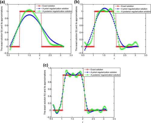
Consider a piecewise smooth source:(5.6) $$\begin{array}{c}\hfill f(r)=\left\{\begin{array}{cc}0,\hfill & 0\le r\le \frac{\mathit{\pi }}{4},\hfill \\ \frac{4}{\mathit{\pi }}(r-\frac{\mathit{\pi }}{4}),\hfill & \frac{\mathit{\pi }}{4}<r\le \frac{\mathit{\pi }}{2},\hfill \\ -\frac{4}{\mathit{\pi }}(r-\frac{3\mathit{\pi }}{4}),\hfill & \frac{\mathit{\pi }}{2}<r\le \frac{3\mathit{\pi }}{4},\hfill \\ 0,\hfill & \frac{3\mathit{\pi }}{4}<r\le \mathit{\pi }.\hfill \end{array}\right.\end{array}$$(5.6)

Example 3:

Consider the following discontinuous function:(5.7) $$\begin{array}{c}\hfill f(r)=\left\{\begin{array}{cc}0,\hfill & 0\le r\le \frac{\mathit{\pi }}{3},\hfill \\ 1,\hfill & \frac{\mathit{\pi }}{3}<r\le \frac{2\mathit{\pi }}{3},\hfill \\ 0,\hfill & \frac{2\mathit{\pi }}{3}<r\le \mathit{\pi }.\hfill \end{array}\right.\end{array}$$(5.7)

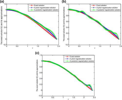
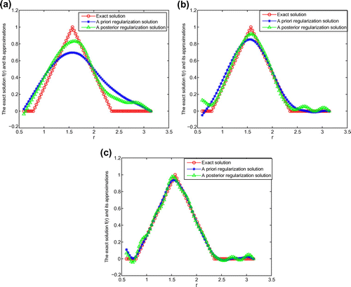
From Figures 3–5, we can see that the smaller $\mathit{\epsilon }$, the better the computed approximation is. Moreover, we can see that the a posteriori parameter choice also works well. In Examples 2–3, since the direct problem with the source f(r) does not have an explicit solution, the data g(r) are obtained by solving the direct problem. Figure 4 shows the comparisons between the exact solution and its computed approximation with different noise levels for Example 2. Figure 5 indicates the comparisons between the exact solution and its computed approximation with different noise levels for Example 3. From Figures 4–5, it can be seen that the numerical solution is less ideal than that of Example 1. Because in examples 2, 3, the exact solutions are non-smooth and discontinuities functions, the recover data near the non-smooth and discontinuities points are not accurate. This is the well-known Gibbs phenomenon. But considered the ill-posed problem, the results presented in Figures 4 and 5 are reasonable.

6. Conclusion

In this paper, we propose an efficient regularization method for identifying a space-dependent source. Under the a priori condition, we give the optimal error bound for this problem. Moreover, we obtain the stability estimate using the conditional stability. Thirdly, under a priori and a posteriori parameter choice rules, we all obtain the order-optimal error estimates. Finally, the numerical experiments show this proposed method works effectively.

Additional information

Funding

The project is supported by the National Natural Science Foundation of China [grant number 11561045], [grant number 11501272]; the Doctor Fund of Lan Zhou University of Technology.

Notes

No potential conflict of interest was reported by the authors.

References

- Li GS, Tan YJ, Cheng J, et al. Determining magnitude of groundwater pollution sources by data compatibility analysis. Inverse Probl Sci Eng. 2006;14:287–300.
- Bao G, Ehlers TA, Li PJ. Radiogenic source identification for the helium production-diffusion equation. Commun Comput Phys. 2013;14:1–20.
- Bao G, Dou Y, Ehlers TA, et al. Quantifying tectonic and geomorphic interpretations of thermochronometer data with inverse problem theory. Commun Comput Phys. 2011;9:129–146.
- Wolf RA, Farley KA, Kass DM. Modeling of the temperature sensitivity of the apatite (U – Th)/He thermochronometer. Chem Geol. 1998;148:105–114.
- Ma YJ, Fu CL, Zhang YX. Identification of an unknown source depending on both time and space variables by a variational method. Appl Math Model. 2012;36:5080–5090.
- Liu CS. A two-stage LGSM to identify time-dependent heat source through an internal measurement of temperature. Int. J Heat Mass Transfer. 2009;52:1635–1642.
- Yamamoto M. Conditional stability in determination of densities of heat sources in a bounded domain. Int Ser Numer Math. 1994;18:359–370.
- Hasanov A. Identification of spacewise and time dependent source terms in 1D heat conduction equation from temperature measurement at a final time. Int J Heat Mass Transfer. 2012;55:2069–2080.
- Trong DD, Long NT, Alain PND. Nonhomogeneous heat equation: identification and regularization for the inhomogeneous term. J Math Anal Appl. 2005;312:93–104.
- Yi Z, Murio DA. Identification of source terms in 2-D IHCP. Comput Math Appl. 2004;47:1517–1533.
- El Badia A, Ha-Duong T, Hamdi A. Identification of a point source in a linear advection-dispersion-reaction equation: application to a pollution source problem. Inverse Probl. 2005;21:1121–1136.
- Ismailov MI, Kanca F, Lesnic D. Determination of a time-dependent heat source under nonlocal boundary and integral overdetermination conductions. Appl Math Comput. 2011;218:4138–4146.
- Farcas A, Lesnic D. The boundary-element method for the determination of a heat source dependent on one variable. J Eng Math. 2006;54:375–388.
- Johansson T, Lesnic D. Determination of a spacewise dependent heat source. J Comput Appl Math. 2007;209:66–80.
- Nili Ahmadabadi M, Arab M, Maalek Ghaini FM. The method of fundamental solutions for the inverse space-dependent heat source problem. Eng Anal Bound Elem. 2009;33:1231–1235.
- Yang L, Deng ZC, Yu JN, et al. Optimization method for the inverse problem of reconstructing the source term in a parabolic equation. Math Comput Simul. 2009;80:314–326.
- Yang L, Dehghan M, Yu JN, et al. Inverse problem of time-dependent heat sources numerical reconstruction. Math Comput Simul. 2011;81:1656–1672.
- Yan L, Fu CL, Yang FL. The method of fundamental solutions for the inverse heat source problem. Eng Anal Bound Elem. 2008;32:216–222.
- Liu CH. A two-stage LGSM to identify time-dependent heat source through an internal measurement of temperature. Int J Heat Mass Transfer. 2009;52:1635–1642.
- Wei T, Wang JC. Simultaneous determination for a space-dependent heat source and the initial data by the MFS. Eng Anal Bound Elem. 2012;36:1848–1855.
- Liu FB. A modified genetic algorithm for solving the inverse heat transfer problem of estimating plan heat source. Int J Heat Mass Transfer. 2008;51:3745–3752.
- Yan L, Fu CL, Dou FF. A computational method for identifying a spacewise-dependent heat source. Commun Numer Meth Eng. 2010;26:597–608.
- Yan L, Yang FL, Fu CL. A meshless method for solving an inverse spacewise-dependent heat source problem. J Comput Phys. 2009;228:123–136.
- Zhao ZY, Xie O, You L, et al. A truncation method based on hermite expansion for unknown source in space fractional diffusion equation. Math Model Anal. 2014;19(3):430–442.
- Dou FF, Fu CL. Determining an unknown source in the heat equation by a wavelet dual least squares method. Appl Math Lett. 2009;22:661–667.
- Dou FF, Fu CL, Yang FL. Optimal error bound and Fourier regularization for identifying an unknown source in the heat equation. J Comput Appl Math. 2009;230:728–737.
- Yang F, Fu CL. A simplified Tikhonov regularization method for determining the heat source. Appl Math Model. 2010;34:3286–3299.
- Yang F, Fu CL. The method of simplified Tikhonov regularization for dealing with the inverse time-dependent heat source problem. Comput Math Appl. 2010;60:1228–1236.
- Yang F, Fu CL. Two regularization methods for identification of the heat source depending only on spatial variable for the heat equation. J Inv Ill-Posed Probl. 2009;17:815–830.
- Li XX, Yang F. The truncation method for identifying the heat source dependent on a spatial variable. Comput Math Appl. 2011;62:2497–2505.
- Yang F, Fu CL. Two regularization methods to identify time-dependent heat source through an internal measurement of temperature. Math Comput Model. 2011;53:793–804.
- Dou FF, Fu CL, Yang F. Identifying an unknown source term in a heat equation. Inverse Probl Sci Eng. 2009;17:901–913.
- Yang L, Yu JN, Luo GW, et al. Numerical identification of source terms for a two dimensional heat conduction problem in polar coordinate system. Appl Math Model. 2013;37:939–957.
- D’haeyer S, Johansson BT, Slodicka M. Reconstruction of a spacewise-dependent heat source in a time-dependent heat diffusion process. IMA J Appl Math. 2014;79(1):33–53.
- Cheng W, Fu CL. Identifying an unknown source term in a spherically symmetric parabolic equation. Appl Math Lett. 2013;26:387–391.
- Cheng W, Ma YJ, Fu CL. Identifying an unknown source term in radial heat conduction. Inverse Probl Sci Eng. 2012;20:335–349.
- Liu JJ, Yamamoto M. A backward problem for the time-fractional diffusion equation. Appl Anal. 2010;89(11):1769–1788.
- Wang JG, Wei T, Zhou YB. Tikhonov regularization method for a backward problem for the time-fractional diffusion equation. Appl Math Model. 2013;37:8518–8532.
- Kirsch A. An introduction to the mathematical theory of inverse problems. New York (NY): Springer-Verlag; 1996.
- Ivanchov MI. The inverse problem of determining the heat source power for a parabolic equation under arbitrary boundary conditions. J Math Sci. 1998;88:432–436.
- Schröer T, Tautenhahn U. On the ‘optimal’ regularization methods for solving linear ill-posed problems. Z Anal Anwend. 1994;13:697–710.
- Tautenhahn U. Optimal stable approximations for the sideways heat equation. J Inverse Ill-Posed Probl. 1997;5:287–307.
- Tautenhahn U. Optimality for ill-posed problems under general source conditions. Numer Funct Anal Optim. 1998;19:377–398.
- Vainikko G. On the optimality of methods for ill-posed problems. Z Anal Anwend. 1987;64:351–362.
- Tautenhahn U, Gorenflo R. On optimal regularization methods for fractional differentiation. J Anal Appl. 1999;18:449–467.
- Cheng W, Zhao LL, Fu CL. Source term identification for an axisymmetric inverse heat conduction. Comput Math Appl. 2010;59:142–148.