Simultaneous reconstruction of the time-dependent Robin coefficient and heat flux in heat conduction problems

Abstract

This paper aims to solve an inverse heat conduction problem in two-dimensional space under transient regime, which consists of the estimation of multiple time-dependent heat sources placed at the boundaries. Robin boundary condition (third type boundary condition) is considered at the working domain boundary. The simultaneous identification problem is formulated as a constrained minimization problem using the output least squares method with Tikhonov regularization. The properties of the continuous and discrete optimization problem are studied. Differentiability results and the adjoint problems are established. The numerical estimation is investigated using a modified conjugate gradient method. Furthermore, to verify the performance of the proposed algorithm, obtained results are compared with results obtained from the well-known finite-element software COMSOL Multiphysics under the same conditions. The numerical results show that the proposed algorithm is accurate, robust and capable of simultaneously representing the time effects on reconstructing the time-dependent Robin coefficient and heat flux.

Keywords:

• Inverse heat conduction problem
• numerical reconstruction
• modified conjugate gradient method
• Tikhonov’s regularization

AMS Subject Classifications:

• 34K28
• 34K29
• 65L20

1. Introduction

In general, heat transfer problems are classified as direct or inverse. In direct problems, prediction of temperature field within a predefined physical domain requires full information about the material thermo-physical properties, domain geometry, internal heat sources, initial conditions and boundary conditions. The inverse problems, generally, arise when at least one of the above-mentioned inputs is not known a priori and is to be determined using measured temperature data-sets at a single or several locations of the physical domain. Háo et al. [1] investigated the inverse problem for determining the heat transfer coefficient considering the third-kind Robin boundary condition in transient heat conduction for both space or time-dependencies using least-squares penalized variational formulations. Furthermore, [2] considered determination of both space or time-dependent ambient temperature of the third-kind Robin boundary condition in transient heat conduction based on surface temperature measurements. Martin and Dulikravich [3] studied an experimental set-up for determining the heat transfer coefficient and investigated its sensitivity with respect to experimental uncertainties using the boundary element method. Háo et al. [4] investigated the problem of identifying non-linear heat transfer laws at the boundary of the temperature-dependent heat transfer coefficient in a parabolic equation from boundary observations. That model applies to the heat transfer coefficient that describes the intensity of heat exchange between a hot wire and the cooling water. Inverse heat conduction problems (IHCP) are mathematically considered as ill-posed problems as they are very sensitive to temperature measurement errors [5]. IHCP represent the reconstruction of the heat flux and Robin coefficient of a heat conducting body. Transient temperature measurements inside the body are utilized in the calculational procedure. The presence of errors in the measurements as well as the ill-posed nature of the problem lead to "reconstruction" rather than the "true" heat flux, Robin coefficient and/or temperature [6]. A lot of classical methods have been developed to solve this IHCP such as maximum entropy principle [7], conjugate gradient method (CGM) [8], Tikhonov regularization and truncated singular value decomposition [9]. Levenberg–Marquardt method has been widely used to find a solution of a constrained system of non-linear equations (see, e.g. [10,11]). Most of the studies based on the above-mentioned methods are focused on steady-state problems with constant intensity heat source [12].

Why the parameters (heat transfer coefficient and heat flux) to be reconstructed are dependent on time t? Briefly, the total heat transfer from a certain domain to its surroundings depends on many factors two of which are easily known: temperature difference and area. While the area is constant, the ambient temperature may be considered as time dependent [13–15]. Moreover, the heat transfer coefficient depends on many factors such as velocity of the fluid [16], fluid properties (viscosity, density, and thermal conductivity), and orientation of the flow. All these factors may vary with time in many real-life applications [17] and hence the convective heat transfer coefficient changes with time. The heat flux depends on time in several applications such as metal machining with variable cutting parameters [18] and identification of a high-magnitude boundary heat flux on a plate [19].

COMSOL Multiphysics is (in general) a finite-element analysis solver and simulation software used for various physics and engineering applications [20]. It was used for solving many inverse problems in literature. Cardiffa and Kitanidis [21] presented a framework for the solution of underdetermined inverse problems using COMSOL Multiphysics that is applicable to a broad range of physical systems governed by PDEs. Brito et al. [22] proposed the use of a non-linear inverse problem technique in connection with COMSOL to estimate the heat flux and the temperature field on turning cutting tool in transient regime. Sousa et al. [23] performed temperature measurements using infrared thermography on 3D surfaces in combination with an inverse heat conduction method, which was solved using CGM, coupled with COMSOL. Li et al. [24] constructed a parameter inverse analysis model for the diffusion analysis experiments of multi-ion transport model using COMSOL Multiphysics linked to Matlab.

Onyango et al. [25] studied the one-dimensional transient inverse heat conduction problem for reconstructing the heat transfer coefficient for both space or time dependencies from surface temperature or average temperature measurements. The numerical boundary element method produced convergent and stable numerical results. Furthermore, a restoration of boundary conditions in one-dimensional transient inverse heat-conduction problems is investigated in [26]. The boundary conditions are represented by linear relations between the temperature and the heat flux, together with an initial condition as a function of space. Jin and Lu [27] studied the numerical reconstruction of the Robin coefficient in the parabolic problems and investigated the convergence analysis and stability of the approximations. Levenberg–Marquardt algorithm was modified in [28] to simultaneously estimate multi-parameters of boundary heat flux by solving transient non-linear IHCP. Our previous work [29] focused on the numerical reconstruction of the spatially-dependent Robin coefficient and heat flux simultaneously using Levenberg–Marquardt and surrogate functional method. Recently, Abdelhamid Talaat [30] studied the simultaneously identification of the spatio-temporal dependent heat transfer coefficient $\mathit{\gamma }(\mathbf{x},t)$ and the spatially dependent heat flux q(x) in a parabolic system. Abdelhamid et al. [31] introduced a regularization approach for simultaneously reconstructing the space-time dependent Robin coefficient $\mathit{\gamma }(\mathbf{x},t)$ and space-time dependent heat flux $q(\mathbf{x},t)$. The present study is based on simultaneously reconstructing the time-dependent Robin coefficient and the time-dependent heat flux using a modified CGM. The obtained results are then compared with those obtained by COMSOL software.

The rest of the paper is organized as follows. In Section 2, the mathematical and variational formulation of the parabolic inverse problem are introduced. In Section 3 the Tikhonov regularization method is adopted to cope with the uncontrollable effect of noise. Section 4 investigates the differentiability results to obtain the gradient of the Robin coefficient and heat flux and derives the adjoint problems to find simple explicit relations that simplify computing the step lengths. Section 5 discusses the numerical algorithm using the modified CGM. Section 6 presents the numerical results of the proposed method compared to the results obtained from the well-known finite-element software COMSOL Multiphysics under the same conditions to show the efficiency and the accuracy of the proposed algorithm.

2. Mathematical formulation

Let $\mathrm{\Omega }\subset R^{♭}$ $(♭\ge 2)$ be an open, bounded and connected domain with sufficiently smooth boundary $\mathit{\partial }\mathrm{\Omega }$. Consider the following parabolic system:(2.1) $$\begin{array}{c}\hfill \left\{\begin{array}{cc}\frac{\mathit{\partial }T}{\mathit{\partial }t}-\mathcal{D}{\mathrm{\nabla }}^{2}T=f(\mathbf{x},t)\hfill & \text{in}\mathrm{\Omega }\times (0,\tilde{t}),\hfill \\ \hfill \\ \mathit{\alpha }\frac{\mathit{\partial }T}{\mathit{\partial }n}+\mathit{\gamma }(t)T(\mathbf{x},t)=g(\mathbf{x},t)\hfill & \text{on}{\mathrm{\Gamma }}_i\times (0,\tilde{t}),\hfill \\ \hfill \\ \mathit{\alpha }\frac{\mathit{\partial }T}{\mathit{\partial }n}=Q(t)h(\mathbf{x},t)\hfill & \text{on}{\mathrm{\Gamma }}_c\times (0,\tilde{t}),\hfill \\ \hfill \\ T(\mathbf{x},0)=T_0(\mathbf{x})\hfill & \text{in}\overline{\mathrm{\Omega }}.\hfill \end{array}\right.\end{array}$$(2.1)

We assume that the whole boundary $\mathit{\partial }\mathrm{\Omega }$ consists of two parts ${\mathrm{\Gamma }}_i$ and ${\mathrm{\Gamma }}_c$. Here $\mathit{\rho }$, c, and $\mathit{\alpha }$ are the specific heat, density and thermal diffusivity, respectively, and $\mathcal{D}=\mathit{\alpha }/\mathit{\rho }c$ is assumed to be given positive constants. Also, the Robin coefficient $\mathit{\gamma }(t)$ and heat flux Q(t) are included in the following constrained sets$$\begin{array}{cc}\hfill K_1& =\{\mathit{\gamma }(t)\in L^2(0,\tilde{t}):0<{\mathit{\gamma }}_1\le \mathit{\gamma }(t)\le {\mathit{\gamma }}_2<\infty \text{a.e. on}(0,\tilde{t})\},\hfill \\ \hfill K_2& =\{Q(t)\in L^2(0,\tilde{t}):0<r_1\le Q(t)\le r_2<\infty \text{a.e. on}(0,\tilde{t})\},\hfill \end{array}$$

where the constrains ${\mathit{\gamma }}_1,{\mathit{\gamma }}_2,r_1$, and $r_2$ are known positive constants. We assume that the heat flux is constrained by $r_1$ and $r_2$ which are positive lower and upper bounds, respectively, to guarantee the boundedness of the solution. In addition, we can assume that the heat flux moves from higher temperature regions (ambient temperature) to lower temperature regions (domain temperature) in the positive direction of x-axis. Let $T(\mathbf{x},t)$ solve system (2.1(2.1) $$\begin{array}{c}\hfill \left\{\begin{array}{cc}\frac{\mathit{\partial }T}{\mathit{\partial }t}-\mathcal{D}{\mathrm{\nabla }}^{2}T=f(\mathbf{x},t)\hfill & \text{in}\mathrm{\Omega }\times (0,\tilde{t}),\hfill \\ \hfill \\ \mathit{\alpha }\frac{\mathit{\partial }T}{\mathit{\partial }n}+\mathit{\gamma }(t)T(\mathbf{x},t)=g(\mathbf{x},t)\hfill & \text{on}{\mathrm{\Gamma }}_i\times (0,\tilde{t}),\hfill \\ \hfill \\ \mathit{\alpha }\frac{\mathit{\partial }T}{\mathit{\partial }n}=Q(t)h(\mathbf{x},t)\hfill & \text{on}{\mathrm{\Gamma }}_c\times (0,\tilde{t}),\hfill \\ \hfill \\ T(\mathbf{x},0)=T_0(\mathbf{x})\hfill & \text{in}\overline{\mathrm{\Omega }}.\hfill \end{array}\right.\end{array}$$(2.1) ), $z^{\mathit{\varrho }}\in L^2(0,\tilde{t};L^2({\mathrm{\Gamma }}_c))$ is the measured data taken on the accessible boundary ${\mathrm{\Gamma }}_c$ over $t\in (0,\tilde{t})$, and $T_0$ is given function. The parameter $\mathit{\varrho }$ is used to denote noise in the measured data.

Lemma 2.1:

[27]] The norm ${\Vert ·\Vert }_{1,{\mathrm{\Gamma }}_i}$ defined by$$\begin{array}{c}\hfill {\Vert T\Vert }_{1,{\mathrm{\Gamma }}_i}^2={\Vert \mathrm{\nabla }T\Vert }_{L^2(\mathrm{\Omega })}^2+{\Vert T\Vert }_{L^2({\mathrm{\Gamma }}_i)}^2,\end{array}$$

is equivalent to the standard norm ${\Vert T\Vert }_{H^1(\mathrm{\Omega })}^2$.

The following assumption is set to state the well-posedness of the forward solution $T(\mathbf{x},t)$ of system (2.1(2.1) $$\begin{array}{c}\hfill \left\{\begin{array}{cc}\frac{\mathit{\partial }T}{\mathit{\partial }t}-\mathcal{D}{\mathrm{\nabla }}^{2}T=f(\mathbf{x},t)\hfill & \text{in}\mathrm{\Omega }\times (0,\tilde{t}),\hfill \\ \hfill \\ \mathit{\alpha }\frac{\mathit{\partial }T}{\mathit{\partial }n}+\mathit{\gamma }(t)T(\mathbf{x},t)=g(\mathbf{x},t)\hfill & \text{on}{\mathrm{\Gamma }}_i\times (0,\tilde{t}),\hfill \\ \hfill \\ \mathit{\alpha }\frac{\mathit{\partial }T}{\mathit{\partial }n}=Q(t)h(\mathbf{x},t)\hfill & \text{on}{\mathrm{\Gamma }}_c\times (0,\tilde{t}),\hfill \\ \hfill \\ T(\mathbf{x},0)=T_0(\mathbf{x})\hfill & \text{in}\overline{\mathrm{\Omega }}.\hfill \end{array}\right.\end{array}$$(2.1) ) (see, Theorem 2.4 [32]).

Assumption 2.1:

Suppose that $f(\mathbf{x},t)\in L^2(0,\tilde{t};L^2(\mathrm{\Omega }))$, $g(\mathbf{x},t)\in L^2(0,\tilde{t};L^2({\mathrm{\Gamma }}_i))$ and $h(\mathbf{x},t)\in L^2(0,\tilde{t};L^2({\mathrm{\Gamma }}_c))$.

Lemma 2.2:

Let Assumption 2.1 hold. For any $(\mathit{\gamma },Q)\in K_1\times K_2$, there exists a unique solution $T(\mathit{\gamma },Q)(\mathbf{x},t)\equiv T(\mathit{\gamma },Q)\in L^2(0,\tilde{t};H^1(\mathrm{\Omega }))$ to system (2.1(2.1) $$\begin{array}{c}\hfill \left\{\begin{array}{cc}\frac{\mathit{\partial }T}{\mathit{\partial }t}-\mathcal{D}{\mathrm{\nabla }}^{2}T=f(\mathbf{x},t)\hfill & \text{in}\mathrm{\Omega }\times (0,\tilde{t}),\hfill \\ \hfill \\ \mathit{\alpha }\frac{\mathit{\partial }T}{\mathit{\partial }n}+\mathit{\gamma }(t)T(\mathbf{x},t)=g(\mathbf{x},t)\hfill & \text{on}{\mathrm{\Gamma }}_i\times (0,\tilde{t}),\hfill \\ \hfill \\ \mathit{\alpha }\frac{\mathit{\partial }T}{\mathit{\partial }n}=Q(t)h(\mathbf{x},t)\hfill & \text{on}{\mathrm{\Gamma }}_c\times (0,\tilde{t}),\hfill \\ \hfill \\ T(\mathbf{x},0)=T_0(\mathbf{x})\hfill & \text{in}\overline{\mathrm{\Omega }}.\hfill \end{array}\right.\end{array}$$(2.1) ). Moreover, it satisfies the following estimate:$$\begin{array}{c}\hfill {\Vert T(\mathit{\gamma },Q)\Vert }_{L^2(0,\tilde{t};H^1(\mathrm{\Omega }))}\le C\left({\Vert f\Vert }_{L^2(0,\tilde{t};L^2(\mathrm{\Omega }))}+{\Vert g\Vert }_{L^2(0,\tilde{t};L^2({\mathrm{\Gamma }}_i))}+{\Vert h\Vert }_{L^2(0,\tilde{t};L^2({\mathrm{\Gamma }}_c))}\right).\end{array}$$

Then, from Lemmas 2.1 and 2.2 we deduce that the solution $T(\mathit{\gamma },Q)$ of system (2.1(2.1) $$\begin{array}{c}\hfill \left\{\begin{array}{cc}\frac{\mathit{\partial }T}{\mathit{\partial }t}-\mathcal{D}{\mathrm{\nabla }}^{2}T=f(\mathbf{x},t)\hfill & \text{in}\mathrm{\Omega }\times (0,\tilde{t}),\hfill \\ \hfill \\ \mathit{\alpha }\frac{\mathit{\partial }T}{\mathit{\partial }n}+\mathit{\gamma }(t)T(\mathbf{x},t)=g(\mathbf{x},t)\hfill & \text{on}{\mathrm{\Gamma }}_i\times (0,\tilde{t}),\hfill \\ \hfill \\ \mathit{\alpha }\frac{\mathit{\partial }T}{\mathit{\partial }n}=Q(t)h(\mathbf{x},t)\hfill & \text{on}{\mathrm{\Gamma }}_c\times (0,\tilde{t}),\hfill \\ \hfill \\ T(\mathbf{x},0)=T_0(\mathbf{x})\hfill & \text{in}\overline{\mathrm{\Omega }}.\hfill \end{array}\right.\end{array}$$(2.1) ) is well-defined to $L^2(0,\tilde{t};H^1(\mathrm{\Omega }))$. The purpose of this study is to identify the time-dependent functions $\mathit{\gamma }(t)\in K_1$ and $Q(t)\in K_2$ and the temperature $T(\mathit{\gamma },Q)$ satisfying (2.1(2.1) $$\begin{array}{c}\hfill \left\{\begin{array}{cc}\frac{\mathit{\partial }T}{\mathit{\partial }t}-\mathcal{D}{\mathrm{\nabla }}^{2}T=f(\mathbf{x},t)\hfill & \text{in}\mathrm{\Omega }\times (0,\tilde{t}),\hfill \\ \hfill \\ \mathit{\alpha }\frac{\mathit{\partial }T}{\mathit{\partial }n}+\mathit{\gamma }(t)T(\mathbf{x},t)=g(\mathbf{x},t)\hfill & \text{on}{\mathrm{\Gamma }}_i\times (0,\tilde{t}),\hfill \\ \hfill \\ \mathit{\alpha }\frac{\mathit{\partial }T}{\mathit{\partial }n}=Q(t)h(\mathbf{x},t)\hfill & \text{on}{\mathrm{\Gamma }}_c\times (0,\tilde{t}),\hfill \\ \hfill \\ T(\mathbf{x},0)=T_0(\mathbf{x})\hfill & \text{in}\overline{\mathrm{\Omega }}.\hfill \end{array}\right.\end{array}$$(2.1) ) and(2.2) $$\begin{array}{c}\hfill T(\mathbf{x},t)=z^{\mathit{\varrho }}(\mathbf{x},t)\text{on}{\mathrm{\Gamma }}_c\times (0,\tilde{t}).\end{array}$$(2.2)

The uniqueness of solution and stability to this inverse problem remain open issues.

3. Tikhonov’s regularization

Tikhonov’s regularization for the proposed inverse problem requires minimizing(3.1) $$\begin{array}{c}\hfill \underset{(\mathit{\gamma },Q)\in K_1\times K_2}{min}J(\mathit{\gamma },Q)=\underset{(\mathit{\gamma },Q)}{min}\left[\frac{1}{2}{\int }_0^{\tilde{t}}\Vert T(\mathit{\gamma },Q)-z^{\mathit{\varrho }}{\Vert }_{L^2({\mathrm{\Gamma }}_c)}^2\mathrm{d}t+\frac{\mathit{\beta }}{2}{\Vert \mathit{\gamma }\Vert }_{L^2(0,\tilde{t})}^2+\frac{\mathit{\eta }}{2}{\Vert Q\Vert }_{L^2(0,\tilde{t})}^2\right],\end{array}$$(3.1)

where $T\equiv T(\mathit{\gamma },Q)(\mathbf{x},t)\in L^2(0,\tilde{t};H^1(\mathrm{\Omega }))$ satisfies(3.2) $$\begin{array}{c}\hfill T(\mathbf{x},0)=T_0(\mathbf{x})\text{in}\mathrm{\Omega },\end{array}$$(3.2)

and(3.3) $$\begin{array}{c}\hfill {\int }_0^{\tilde{t}}{\int }_{\mathrm{\Omega }}{\mathit{\partial }}_{t}Tv\mathrm{d}x\mathrm{d}t+{\int }_0^{\tilde{t}}{\int }_{\mathrm{\Omega }}\mathrm{\nabla }T·\mathrm{\nabla }v\mathrm{d}x\mathrm{d}t+{\int }_0^{\tilde{t}}{\int }_{{\mathrm{\Gamma }}_i}\mathit{\gamma }Tv\mathrm{d}s\mathrm{d}t={\int }_0^{\tilde{t}}{\int }_{\mathrm{\Omega }}fv\mathrm{d}x\mathrm{d}t\\ \hfill +{\int }_0^{\tilde{t}}{\int }_{{\mathrm{\Gamma }}_i}gv\mathrm{d}s\mathrm{d}t+{\int }_0^{\tilde{t}}{\int }_{{\mathrm{\Gamma }}_c}Qhv\mathrm{d}s\mathrm{d}t,\forall v\in L^2(0,\tilde{t};H^1(\mathrm{\Omega })).\end{array}$$(3.3)

Also, $\mathit{\beta }$ and $\mathit{\eta }>0$ are regularization parameters to be prescribed. In this paper, we assume that the specific heat, density and thermal conductivity are given constants set to equal one. The objective functional (3.1(3.1) $$\begin{array}{c}\hfill \underset{(\mathit{\gamma },Q)\in K_1\times K_2}{min}J(\mathit{\gamma },Q)=\underset{(\mathit{\gamma },Q)}{min}\left[\frac{1}{2}{\int }_0^{\tilde{t}}\Vert T(\mathit{\gamma },Q)-z^{\mathit{\varrho }}{\Vert }_{L^2({\mathrm{\Gamma }}_c)}^2\mathrm{d}t+\frac{\mathit{\beta }}{2}{\Vert \mathit{\gamma }\Vert }_{L^2(0,\tilde{t})}^2+\frac{\mathit{\eta }}{2}{\Vert Q\Vert }_{L^2(0,\tilde{t})}^2\right],\end{array}$$(3.1) ) consists of two parts, the first is the error term to approach the true solution while the second represents two terms for regularizing the parameters to stabilize the resolution process of the output least squares formulation.

The following theorem gives the existence of a minimizer to the problem (3.1(3.1) $$\begin{array}{c}\hfill \underset{(\mathit{\gamma },Q)\in K_1\times K_2}{min}J(\mathit{\gamma },Q)=\underset{(\mathit{\gamma },Q)}{min}\left[\frac{1}{2}{\int }_0^{\tilde{t}}\Vert T(\mathit{\gamma },Q)-z^{\mathit{\varrho }}{\Vert }_{L^2({\mathrm{\Gamma }}_c)}^2\mathrm{d}t+\frac{\mathit{\beta }}{2}{\Vert \mathit{\gamma }\Vert }_{L^2(0,\tilde{t})}^2+\frac{\mathit{\eta }}{2}{\Vert Q\Vert }_{L^2(0,\tilde{t})}^2\right],\end{array}$$(3.1) )–(3.3(3.3) $$\begin{array}{c}\hfill {\int }_0^{\tilde{t}}{\int }_{\mathrm{\Omega }}{\mathit{\partial }}_{t}Tv\mathrm{d}x\mathrm{d}t+{\int }_0^{\tilde{t}}{\int }_{\mathrm{\Omega }}\mathrm{\nabla }T·\mathrm{\nabla }v\mathrm{d}x\mathrm{d}t+{\int }_0^{\tilde{t}}{\int }_{{\mathrm{\Gamma }}_i}\mathit{\gamma }Tv\mathrm{d}s\mathrm{d}t={\int }_0^{\tilde{t}}{\int }_{\mathrm{\Omega }}fv\mathrm{d}x\mathrm{d}t\\ \hfill +{\int }_0^{\tilde{t}}{\int }_{{\mathrm{\Gamma }}_i}gv\mathrm{d}s\mathrm{d}t+{\int }_0^{\tilde{t}}{\int }_{{\mathrm{\Gamma }}_c}Qhv\mathrm{d}s\mathrm{d}t,\forall v\in L^2(0,\tilde{t};H^1(\mathrm{\Omega })).\end{array}$$(3.3) ).

Theorem 3.1:

[29]]There exists at least a minimizer to the optimization problem (3.1(3.1) $$\begin{array}{c}\hfill \underset{(\mathit{\gamma },Q)\in K_1\times K_2}{min}J(\mathit{\gamma },Q)=\underset{(\mathit{\gamma },Q)}{min}\left[\frac{1}{2}{\int }_0^{\tilde{t}}\Vert T(\mathit{\gamma },Q)-z^{\mathit{\varrho }}{\Vert }_{L^2({\mathrm{\Gamma }}_c)}^2\mathrm{d}t+\frac{\mathit{\beta }}{2}{\Vert \mathit{\gamma }\Vert }_{L^2(0,\tilde{t})}^2+\frac{\mathit{\eta }}{2}{\Vert Q\Vert }_{L^2(0,\tilde{t})}^2\right],\end{array}$$(3.1) )–(3.3(3.3) $$\begin{array}{c}\hfill {\int }_0^{\tilde{t}}{\int }_{\mathrm{\Omega }}{\mathit{\partial }}_{t}Tv\mathrm{d}x\mathrm{d}t+{\int }_0^{\tilde{t}}{\int }_{\mathrm{\Omega }}\mathrm{\nabla }T·\mathrm{\nabla }v\mathrm{d}x\mathrm{d}t+{\int }_0^{\tilde{t}}{\int }_{{\mathrm{\Gamma }}_i}\mathit{\gamma }Tv\mathrm{d}s\mathrm{d}t={\int }_0^{\tilde{t}}{\int }_{\mathrm{\Omega }}fv\mathrm{d}x\mathrm{d}t\\ \hfill +{\int }_0^{\tilde{t}}{\int }_{{\mathrm{\Gamma }}_i}gv\mathrm{d}s\mathrm{d}t+{\int }_0^{\tilde{t}}{\int }_{{\mathrm{\Gamma }}_c}Qhv\mathrm{d}s\mathrm{d}t,\forall v\in L^2(0,\tilde{t};H^1(\mathrm{\Omega })).\end{array}$$(3.3) ).

4. Differentiability results and adjoint problem

In this section, we employ the partial Fréchet derivatives of the forward solution $T(\mathit{\gamma },Q)$ and their adjoint equations. We denote the first sensitivity equation by $T_{\mathit{\gamma }}^1\equiv T_{\mathit{\gamma }}^{{}^{\prime }}(\mathit{\gamma },Q)d$ which is the partial Fréchet derivative of the forward solution with respect to $\mathit{\gamma }(t)$ in any direction $d\in L^2(0,\tilde{t})$, which satisfies(4.1) $$\begin{array}{c}\hfill \left\{\begin{array}{cc}\frac{\mathit{\partial }{T}_{\mathit{\gamma }}^1}{\mathit{\partial }t}-\mathrm{\Delta }{T}_{\mathit{\gamma }}^1=0\hfill & \text{in}\mathrm{\Omega }\times (0,\tilde{t}),\hfill \\ \hfill \\ \frac{\mathit{\partial }{T}_{\mathit{\gamma }}^1}{\mathit{\partial }n}+\mathit{\gamma }{T}_{\mathit{\gamma }}^1=-dT(\mathit{\gamma },Q)\hfill & \text{on}{\mathrm{\Gamma }}_i\times (0,\tilde{t}),\hfill \\ \hfill \\ \frac{\mathit{\partial }{T}_{\mathit{\gamma }}^1}{\mathit{\partial }n}=0\hfill & \text{on}{\mathrm{\Gamma }}_c\times (0,\tilde{t}),\hfill \\ \hfill \\ T_{\mathit{\gamma }}^1(\mathbf{x},0)=0\hfill & \text{in}\mathrm{\Omega }.\hfill \end{array}\right.\end{array}$$(4.1)

While the second sensitivity equation denoted by $T_Q^1\equiv T_Q^{{}^{\prime }}(\mathit{\gamma },Q)p$ is the partial Fréchet derivative of the forward solution with respect to Q(t) in any direction $p\in L^2(0,\tilde{t})$, which satisfies(4.2) $$\begin{array}{c}\hfill \left\{\begin{array}{cc}\frac{\mathit{\partial }{T}_Q^1}{\mathit{\partial }t}-\mathrm{\Delta }{T}_Q^1=0\hfill & \text{in}\mathrm{\Omega }\times (0,\tilde{t}),\hfill \\ \hfill \\ \frac{\mathit{\partial }{T}_Q^1}{\mathit{\partial }n}+\mathit{\gamma }{T}_Q^1=0\hfill & \text{on}{\mathrm{\Gamma }}_i\times (0,\tilde{t}),\hfill \\ \hfill \\ \frac{\mathit{\partial }{T}_Q^1}{\mathit{\partial }n}=ph\hfill & \text{on}{\mathrm{\Gamma }}_c\times (0,\tilde{t}),\hfill \\ \hfill \\ T_Q^1(\mathbf{x},0)=0\hfill & \text{in}\mathrm{\Omega },\hfill \end{array}\right.\end{array}$$(4.2)

Here, (4.1(4.1) $$\begin{array}{c}\hfill \left\{\begin{array}{cc}\frac{\mathit{\partial }{T}_{\mathit{\gamma }}^1}{\mathit{\partial }t}-\mathrm{\Delta }{T}_{\mathit{\gamma }}^1=0\hfill & \text{in}\mathrm{\Omega }\times (0,\tilde{t}),\hfill \\ \hfill \\ \frac{\mathit{\partial }{T}_{\mathit{\gamma }}^1}{\mathit{\partial }n}+\mathit{\gamma }{T}_{\mathit{\gamma }}^1=-dT(\mathit{\gamma },Q)\hfill & \text{on}{\mathrm{\Gamma }}_i\times (0,\tilde{t}),\hfill \\ \hfill \\ \frac{\mathit{\partial }{T}_{\mathit{\gamma }}^1}{\mathit{\partial }n}=0\hfill & \text{on}{\mathrm{\Gamma }}_c\times (0,\tilde{t}),\hfill \\ \hfill \\ T_{\mathit{\gamma }}^1(\mathbf{x},0)=0\hfill & \text{in}\mathrm{\Omega }.\hfill \end{array}\right.\end{array}$$(4.1) ) and (4.2(4.2) $$\begin{array}{c}\hfill \left\{\begin{array}{cc}\frac{\mathit{\partial }{T}_Q^1}{\mathit{\partial }t}-\mathrm{\Delta }{T}_Q^1=0\hfill & \text{in}\mathrm{\Omega }\times (0,\tilde{t}),\hfill \\ \hfill \\ \frac{\mathit{\partial }{T}_Q^1}{\mathit{\partial }n}+\mathit{\gamma }{T}_Q^1=0\hfill & \text{on}{\mathrm{\Gamma }}_i\times (0,\tilde{t}),\hfill \\ \hfill \\ \frac{\mathit{\partial }{T}_Q^1}{\mathit{\partial }n}=ph\hfill & \text{on}{\mathrm{\Gamma }}_c\times (0,\tilde{t}),\hfill \\ \hfill \\ T_Q^1(\mathbf{x},0)=0\hfill & \text{in}\mathrm{\Omega },\hfill \end{array}\right.\end{array}$$(4.2) ) are linear with respect to d and p, respectively.

Theorem 4.1:

For any $\mathit{\gamma },\mathit{\gamma }+d\in K_1$ and $Q,Q+p\in K_2$, the mapping $(\mathit{\gamma },Q)⟼T(\mathit{\gamma },Q)$ from $K_1\times K_2\to L^2(0,\tilde{t};H^1(\mathrm{\Omega }))$ is Lipschitz continuity and Fréchet differentiable such that(4.3) $$\begin{array}{c}\hfill \underset{{\Vert d\Vert }_{L^{\infty }(0,\tilde{t})}\to 0}{lim}\frac{\Vert T(\mathit{\gamma }+d,Q)-T(\mathit{\gamma },Q)-T_{\mathit{\gamma }}^1{\Vert }_{L^2(0,\tilde{t};H^1(\mathrm{\Omega }))}}{{\Vert d\Vert }_{L^{\infty }(0,\tilde{t})}}=0,\end{array}$$(4.3)

and(4.4) $$\begin{array}{c}\hfill \underset{{\Vert p\Vert }_{L^{\infty }(0,\tilde{t})}\to 0}{lim}\frac{\Vert T(\mathit{\gamma },Q+p)-T(\mathit{\gamma },Q)-T_Q^1{\Vert }_{L^2(0,\tilde{t};H^1(\mathrm{\Omega }))}}{{\Vert p\Vert }_{L^{\infty }(0,\tilde{t})}}=0.\end{array}$$(4.4)

Proof Let $w_{\mathit{\gamma }}\equiv T(\mathit{\gamma }+d,Q)-T(\mathit{\gamma },Q)-T_{\mathit{\gamma }}^1$ and $\mathit{\delta }{T}_{\mathit{\gamma }}\equiv T(\mathit{\gamma }+d,Q)-T(\mathit{\gamma },Q)$ which satisfy(4.5) $$\begin{array}{c}\hfill \left\{\begin{array}{cc}\frac{\mathit{\partial }{w}_{\mathit{\gamma }}}{\mathit{\partial }t}-\mathrm{\Delta }{w}_{\mathit{\gamma }}=0\hfill & \text{in}\mathrm{\Omega }\times (0,\tilde{t}),\hfill \\ \hfill \\ \frac{\mathit{\partial }{w}_{\mathit{\gamma }}}{\mathit{\partial }n}+\mathit{\gamma }{w}_{\mathit{\gamma }}=-\mathrm{d}\mathit{\delta }{T}_{\mathit{\gamma }}\hfill & \text{on}{\mathrm{\Gamma }}_i\times (0,\tilde{t}),\hfill \\ \hfill \\ \frac{\mathit{\partial }{w}_{\mathit{\gamma }}}{\mathit{\partial }n}=0\hfill & \text{on}{\mathrm{\Gamma }}_c\times (0,\tilde{t}),\hfill \\ \hfill \\ w_{\mathit{\gamma }}(·,0)=0\hfill & \text{in}\mathrm{\Omega }.\hfill \end{array}\right.\end{array}$$(4.5)

Multiplying the first equation by $w_{\mathit{\gamma }}$ and integrating over $\mathrm{\Omega }$ gives(4.6) $$\begin{array}{c}\hfill \frac{1}{2}\frac{\mathrm{d}}{\mathrm{d}t}\Vert w_{\mathit{\gamma }}{(·,t)\Vert }_{L^2(\mathrm{\Omega })}^2+{\int }_{\mathrm{\Omega }}|\mathrm{\nabla }{w}_{\mathit{\gamma }}{|}^2\mathrm{d}x+{\int }_{{\mathrm{\Gamma }}_i}\mathit{\gamma }{|w_{\mathit{\gamma }}|}^2\mathrm{d}s=-{\int }_{{\mathrm{\Gamma }}_i}\mathrm{d}\mathit{\delta }{T}_{\mathit{\gamma }}{w}_{\mathit{\gamma }}\mathrm{d}s.\end{array}$$(4.6)

Using the generalized Hölder’s inequality and integrating with respect to $\tilde{t}$, we obtain(4.7) $$\begin{array}{cc}& \frac{1}{2}\Vert w_{\mathit{\gamma }}(·,\tilde{t}){\Vert }_{L^2(\mathrm{\Omega })}^2+\Vert \mathrm{\nabla }{w}_{\mathit{\gamma }}{\Vert }_{L^2(0,\tilde{t};H^1(\mathrm{\Omega }))}^2+{\mathit{\gamma }}_1{\Vert w_{\mathit{\gamma }}\Vert }_{L^2(0,\tilde{t};L^2({\mathrm{\Gamma }}_i))}^2\hfill \\ \hfill & \le {C\Vert d\Vert }_{L^{\infty }(0,\tilde{t})}\Vert \mathit{\delta }{T}_{\mathit{\gamma }}{\Vert }_{L^2(0,\tilde{t};L^2({\mathrm{\Gamma }}_i))}{\Vert w_{\mathit{\gamma }}\Vert }_{L^2(0,\tilde{t};L^2({\mathrm{\Gamma }}_i))}\hfill \\ \hfill & \le {C\Vert d\Vert }_{L^{\infty }(0,\tilde{t})}\Vert \mathit{\delta }{T}_{\mathit{\gamma }}{\Vert }_{L^2(0,\tilde{t};H^1(\mathrm{\Omega }))}{\Vert w_{\mathit{\gamma }}\Vert }_{L^2(0,\tilde{t};H^1(\mathrm{\Omega }))}.\hfill \end{array}$$(4.7)

From Lemma 2.2 we deduce(4.8) $$\begin{array}{c}\hfill \Vert w_{\mathit{\gamma }}{\Vert }_{L^2(0,\tilde{t};H^1(\mathrm{\Omega }))}^2\le {C\Vert d\Vert }_{L^{\infty }(0,\tilde{t})}\Vert \mathit{\delta }{T}_{\mathit{\gamma }}{\Vert }_{L^2(0,\tilde{t};H^1(\mathrm{\Omega }))}{\Vert w_{\mathit{\gamma }}\Vert }_{L^2(0,\tilde{t};H^1(\mathrm{\Omega }))}.\end{array}$$(4.8)

Then, we obtain(4.9) $$\begin{array}{c}\hfill \Vert w_{\mathit{\gamma }}{\Vert }_{L^2(0,\tilde{t};H^1(\mathrm{\Omega }))}\le {C\Vert d\Vert }_{L^{\infty }(0,\tilde{t})}{\Vert \mathit{\delta }{T}_{\mathit{\gamma }}\Vert }_{L^2(0,\tilde{t};H^1(\mathrm{\Omega }))}.\end{array}$$(4.9)

Replacing $T(\mathit{\gamma },Q)$ with $T(\mathit{\gamma }+d,Q)$ into the forward problem (2.1(2.1) $$\begin{array}{c}\hfill \left\{\begin{array}{cc}\frac{\mathit{\partial }T}{\mathit{\partial }t}-\mathcal{D}{\mathrm{\nabla }}^{2}T=f(\mathbf{x},t)\hfill & \text{in}\mathrm{\Omega }\times (0,\tilde{t}),\hfill \\ \hfill \\ \mathit{\alpha }\frac{\mathit{\partial }T}{\mathit{\partial }n}+\mathit{\gamma }(t)T(\mathbf{x},t)=g(\mathbf{x},t)\hfill & \text{on}{\mathrm{\Gamma }}_i\times (0,\tilde{t}),\hfill \\ \hfill \\ \mathit{\alpha }\frac{\mathit{\partial }T}{\mathit{\partial }n}=Q(t)h(\mathbf{x},t)\hfill & \text{on}{\mathrm{\Gamma }}_c\times (0,\tilde{t}),\hfill \\ \hfill \\ T(\mathbf{x},0)=T_0(\mathbf{x})\hfill & \text{in}\overline{\mathrm{\Omega }}.\hfill \end{array}\right.\end{array}$$(2.1) ) and subtracting from (2.1(2.1) $$\begin{array}{c}\hfill \left\{\begin{array}{cc}\frac{\mathit{\partial }T}{\mathit{\partial }t}-\mathcal{D}{\mathrm{\nabla }}^{2}T=f(\mathbf{x},t)\hfill & \text{in}\mathrm{\Omega }\times (0,\tilde{t}),\hfill \\ \hfill \\ \mathit{\alpha }\frac{\mathit{\partial }T}{\mathit{\partial }n}+\mathit{\gamma }(t)T(\mathbf{x},t)=g(\mathbf{x},t)\hfill & \text{on}{\mathrm{\Gamma }}_i\times (0,\tilde{t}),\hfill \\ \hfill \\ \mathit{\alpha }\frac{\mathit{\partial }T}{\mathit{\partial }n}=Q(t)h(\mathbf{x},t)\hfill & \text{on}{\mathrm{\Gamma }}_c\times (0,\tilde{t}),\hfill \\ \hfill \\ T(\mathbf{x},0)=T_0(\mathbf{x})\hfill & \text{in}\overline{\mathrm{\Omega }}.\hfill \end{array}\right.\end{array}$$(2.1) )(4.10) $$\begin{array}{c}\hfill \frac{1}{2}\Vert \mathit{\delta }{T}_{\mathit{\gamma }}(·,\tilde{t}){\Vert }_{L^2(\mathrm{\Omega })}^2+{\int }_0^{\tilde{t}}{\int }_{\mathrm{\Omega }}|\mathrm{\nabla }\mathit{\delta }{T}_{\mathit{\gamma }}{|}^2\mathrm{d}x\mathrm{d}t+{\mathit{\gamma }}_1{\int }_0^{\tilde{t}}{\int }_{{\mathrm{\Gamma }}_i}{|\mathit{\delta }{T}_{\mathit{\gamma }}|}^2\mathrm{d}s\mathrm{d}t\\ \hfill =-{\int }_0^{\tilde{t}}{\int }_{{\mathrm{\Gamma }}_i}dT(\mathit{\gamma },Q)\mathit{\delta }{T}_{\mathit{\gamma }}\mathrm{d}s\mathrm{d}t.\end{array}$$(4.10)

Using Hölder inequality, Sobolev trace theorem, and Lemma 2.2 we deduce(4.11) $$\begin{array}{c}\hfill \Vert \mathit{\delta }{T}_{\mathit{\gamma }}{\Vert }_{L^2(0,\tilde{t};H^1(\mathrm{\Omega }))}\le {C\Vert d\Vert }_{L^{\infty }(0,\tilde{t})}{\Vert T(\mathit{\gamma },Q)\Vert }_{L^2(0,\tilde{t};H^1(\mathrm{\Omega }))}.\end{array}$$(4.11)

Next, we estimate the time derivative ${\mathit{\partial }}_t{T}_{\mathit{\gamma }}(·,t)$ using the generalized Hölder inequality to show that, it is bounded and independent on $\mathit{\gamma }$ as follows(4.12) $$\begin{array}{cc}\hfill \Vert {\mathit{\partial }}_t(\mathit{\delta }{T}_{\mathit{\gamma }}){\Vert }_{L^2(0,\tilde{t};H^1(\mathrm{\Omega }))}^2& =\underset{{\Vert \mathit{\phi }\Vert }_{L^2(0,\tilde{t};H^1(\mathrm{\Omega }))}=1}{sup}{⟨{\mathit{\partial }}_t\mathit{\delta }{T}_{\mathit{\gamma }},\mathit{\phi }⟩}_{L^2(0,\tilde{t};H^1(\mathrm{\Omega }))}\hfill \\ \hfill & =\underset{{\Vert \mathit{\phi }\Vert }_{L^2(0,\tilde{t};H^1(\mathrm{\Omega }))}=1}{sup}\left\{-{\int }_0^{\tilde{t}}{\int }_{\mathrm{\Omega }}\mathrm{\nabla }\mathit{\delta }{T}_{\mathit{\gamma }}\mathrm{\nabla }\mathit{\phi }\mathrm{d}x\mathrm{d}t\right.\hfill \\ \hfill & \left.-{\int }_0^{\tilde{t}}{\int }_{{\mathrm{\Gamma }}_i}dT\mathit{\phi }\mathrm{d}s\mathrm{d}t-{\int }_0^{\tilde{t}}{\int }_{{\mathrm{\Gamma }}_i}(\mathit{\gamma }+d)\mathit{\delta }{T}_{\mathit{\gamma }}\mathit{\phi }\mathrm{d}s\mathrm{d}t\right\}\hfill \\ \hfill & \le \underset{{\Vert \mathit{\phi }\Vert }_{L^2(0,\tilde{t};H^1(\mathrm{\Omega }))}=1}{sup}\left\{\Vert \mathrm{\nabla }\mathit{\delta }{T}_{\mathit{\gamma }}{\Vert }_{L^2(0,\tilde{t};H^1(\mathrm{\Omega }))}{\Vert \mathrm{\nabla }\mathit{\phi }\Vert }_{L^2(0,\tilde{t};H^1(\mathrm{\Omega }))}\right.\hfill \\ \hfill & +{\Vert d\Vert }_{L^{\infty }(0,\tilde{t})}{\Vert T\Vert }_{L^2(0,\tilde{t};L^2({\mathrm{\Gamma }}_i))}{\Vert \mathit{\phi }\Vert }_{L^2(0,\tilde{t};L^2({\mathrm{\Gamma }}_i))}\hfill \\ \hfill & \left.+c\Vert \mathit{\delta }{T}_{\mathit{\gamma }}{\Vert }_{L^2(0,\tilde{t};L^2({\mathrm{\Gamma }}_i))}{\Vert \mathit{\phi }\Vert }_{L^2(0,\tilde{t};L^2({\mathrm{\Gamma }}_i))}\right\}\hfill \\ \hfill & \le C\left[\Vert \mathit{\delta }{T}_{\mathit{\gamma }}{\Vert }_{L^2(0,\tilde{t};H^1(\mathrm{\Omega }))}+{\Vert d\Vert }_{L^{\infty }(0,\tilde{t})}{\Vert T\Vert }_{L^2(0,\tilde{t};L^2({\mathrm{\Gamma }}_i))}\right]\hfill \\ \hfill & \le {C\Vert d\Vert }_{L^{\infty }(0,\tilde{t})}{\Vert T\Vert }_{L^2(0,\tilde{t};H^1(\mathrm{\Omega }))}.\hfill \end{array}$$(4.12)

Since ${\Vert T(\mathit{\gamma },Q)\Vert }_{L^2(0,\tilde{t};H^1(\mathrm{\Omega }))}$ can be bounded independent of $\mathit{\gamma }\in L^2(0,\tilde{t})$ (see Lemma 2.2), then $\Vert \mathit{\delta }{T}_{\mathit{\gamma }}{\Vert }_{L^2(0,\tilde{t};H^1(\mathrm{\Omega }))}\le C{\Vert d\Vert }_{L^{\infty }(0,\tilde{t})}$. By combining the above estimates (4.9(4.9) $$\begin{array}{c}\hfill \Vert w_{\mathit{\gamma }}{\Vert }_{L^2(0,\tilde{t};H^1(\mathrm{\Omega }))}\le {C\Vert d\Vert }_{L^{\infty }(0,\tilde{t})}{\Vert \mathit{\delta }{T}_{\mathit{\gamma }}\Vert }_{L^2(0,\tilde{t};H^1(\mathrm{\Omega }))}.\end{array}$$(4.9) ), (4.11(4.11) $$\begin{array}{c}\hfill \Vert \mathit{\delta }{T}_{\mathit{\gamma }}{\Vert }_{L^2(0,\tilde{t};H^1(\mathrm{\Omega }))}\le {C\Vert d\Vert }_{L^{\infty }(0,\tilde{t})}{\Vert T(\mathit{\gamma },Q)\Vert }_{L^2(0,\tilde{t};H^1(\mathrm{\Omega }))}.\end{array}$$(4.11) ), and (4.12(4.12) $$\begin{array}{cc}\hfill \Vert {\mathit{\partial }}_t(\mathit{\delta }{T}_{\mathit{\gamma }}){\Vert }_{L^2(0,\tilde{t};H^1(\mathrm{\Omega }))}^2& =\underset{{\Vert \mathit{\phi }\Vert }_{L^2(0,\tilde{t};H^1(\mathrm{\Omega }))}=1}{sup}{⟨{\mathit{\partial }}_t\mathit{\delta }{T}_{\mathit{\gamma }},\mathit{\phi }⟩}_{L^2(0,\tilde{t};H^1(\mathrm{\Omega }))}\hfill \\ \hfill & =\underset{{\Vert \mathit{\phi }\Vert }_{L^2(0,\tilde{t};H^1(\mathrm{\Omega }))}=1}{sup}\left\{-{\int }_0^{\tilde{t}}{\int }_{\mathrm{\Omega }}\mathrm{\nabla }\mathit{\delta }{T}_{\mathit{\gamma }}\mathrm{\nabla }\mathit{\phi }\mathrm{d}x\mathrm{d}t\right.\hfill \\ \hfill & \left.-{\int }_0^{\tilde{t}}{\int }_{{\mathrm{\Gamma }}_i}dT\mathit{\phi }\mathrm{d}s\mathrm{d}t-{\int }_0^{\tilde{t}}{\int }_{{\mathrm{\Gamma }}_i}(\mathit{\gamma }+d)\mathit{\delta }{T}_{\mathit{\gamma }}\mathit{\phi }\mathrm{d}s\mathrm{d}t\right\}\hfill \\ \hfill & \le \underset{{\Vert \mathit{\phi }\Vert }_{L^2(0,\tilde{t};H^1(\mathrm{\Omega }))}=1}{sup}\left\{\Vert \mathrm{\nabla }\mathit{\delta }{T}_{\mathit{\gamma }}{\Vert }_{L^2(0,\tilde{t};H^1(\mathrm{\Omega }))}{\Vert \mathrm{\nabla }\mathit{\phi }\Vert }_{L^2(0,\tilde{t};H^1(\mathrm{\Omega }))}\right.\hfill \\ \hfill & +{\Vert d\Vert }_{L^{\infty }(0,\tilde{t})}{\Vert T\Vert }_{L^2(0,\tilde{t};L^2({\mathrm{\Gamma }}_i))}{\Vert \mathit{\phi }\Vert }_{L^2(0,\tilde{t};L^2({\mathrm{\Gamma }}_i))}\hfill \\ \hfill & \left.+c\Vert \mathit{\delta }{T}_{\mathit{\gamma }}{\Vert }_{L^2(0,\tilde{t};L^2({\mathrm{\Gamma }}_i))}{\Vert \mathit{\phi }\Vert }_{L^2(0,\tilde{t};L^2({\mathrm{\Gamma }}_i))}\right\}\hfill \\ \hfill & \le C\left[\Vert \mathit{\delta }{T}_{\mathit{\gamma }}{\Vert }_{L^2(0,\tilde{t};H^1(\mathrm{\Omega }))}+{\Vert d\Vert }_{L^{\infty }(0,\tilde{t})}{\Vert T\Vert }_{L^2(0,\tilde{t};L^2({\mathrm{\Gamma }}_i))}\right]\hfill \\ \hfill & \le {C\Vert d\Vert }_{L^{\infty }(0,\tilde{t})}{\Vert T\Vert }_{L^2(0,\tilde{t};H^1(\mathrm{\Omega }))}.\hfill \end{array}$$(4.12) ) it follows that (4.3(4.3) $$\begin{array}{c}\hfill \underset{{\Vert d\Vert }_{L^{\infty }(0,\tilde{t})}\to 0}{lim}\frac{\Vert T(\mathit{\gamma }+d,Q)-T(\mathit{\gamma },Q)-T_{\mathit{\gamma }}^1{\Vert }_{L^2(0,\tilde{t};H^1(\mathrm{\Omega }))}}{{\Vert d\Vert }_{L^{\infty }(0,\tilde{t})}}=0,\end{array}$$(4.3) ) is verified. For any Q and $Q+p\in K_2$, we can similarly prove that$$\begin{array}{c}\hfill \Vert \mathit{\delta }{T}_Q{\Vert }_{L^2(0,\tilde{t};H^1(\mathrm{\Omega }))}\le {C\Vert p\Vert }_{L^{\infty }(0,\tilde{t})}{\Vert T(\mathit{\gamma },Q)\Vert }_{L^2(0,\tilde{t};H^1(\mathrm{\Omega }))}.\end{array}$$

Then,$$\begin{array}{c}\hfill \Vert \mathit{\delta }{T}_Q{\Vert }_{L^2(0,\tilde{t};H^1(\mathrm{\Omega }))}\le C{\Vert p\Vert }_{L^{\infty }(0,\tilde{t})}\end{array}$$

and$$\begin{array}{c}\hfill \Vert w_Q{\Vert }_{L^2(0,\tilde{t};H^1(\mathrm{\Omega }))}\le {C\Vert p\Vert }_{L^{\infty }(0,\tilde{t})}{\Vert \mathit{\delta }{T}_Q\Vert }_{L^2(0,\tilde{t};H^1(\mathrm{\Omega }))}.\end{array}$$

The differentiability follows from the Lipschitz continuity of the map $Q\mapsto T(\mathit{\gamma },Q)$; this concludes the proof.

Next, we derive the gradient formula of the functional $J(\mathit{\gamma },Q)$. From Theorem 4.1, we have the following expansions$$\begin{array}{cc}\hfill T(\mathit{\gamma }+d,Q)& =T(\mathit{\gamma },Q)+T_{\mathit{\gamma }}^{{}^{\prime }}(\mathit{\gamma },Q)d+{\mathcal{O}(\Vert d\Vert }_{L^{\infty }(0,\tilde{t})}^2),\hfill \\ \hfill T(\mathit{\gamma },Q+p)& =T(\mathit{\gamma },Q)+T_Q^{{}^{\prime }}(\mathit{\gamma },Q)p+{\mathcal{O}(\Vert p\Vert }_{L^{\infty }(0,\tilde{t})}^2).\hfill \end{array}$$

Now, we define the adjoint equations for the partial Gâteaux derivatives ${\mathit{\omega }}_{\mathit{\gamma }}^{\ast }\equiv T_{\mathit{\gamma }}^{{}^{\prime }}{(\mathit{\gamma },Q)}^{\ast }\mathit{\nu }$ and ${\mathit{\omega }}_Q^{\ast }\equiv T_Q^{{}^{\prime }}{(\mathit{\gamma },Q)}^{\ast }\mathit{\zeta }$ in directions $\mathit{\nu }$ and $\mathit{\zeta }$, respectively. These satisfy the following systems:(4.13) $$\begin{array}{c}\hfill \left\{\begin{array}{cc}\frac{\mathit{\partial }{\mathit{\omega }}_{\mathit{\gamma }}^{\ast }}{\mathit{\partial }t}+\mathrm{\Delta }{\mathit{\omega }}_{\mathit{\gamma }}^{\ast }=0\hfill & \text{in}\mathrm{\Omega }\times (0,\tilde{t}),\hfill \\ \hfill \\ \frac{\mathit{\partial }{\mathit{\omega }}_{\mathit{\gamma }}^{\ast }}{\mathit{\partial }n}+\mathit{\gamma }{\mathit{\omega }}_{\mathit{\gamma }}^{\ast }=0\hfill & \text{on}{\mathrm{\Gamma }}_i\times (0,\tilde{t}),\hfill \\ \hfill \\ \frac{\mathit{\partial }{\mathit{\omega }}_{\mathit{\gamma }}^{\ast }}{\mathit{\partial }n}=-\mathit{\nu }\hfill & \text{on}{\mathrm{\Gamma }}_c\times (0,\tilde{t}),\hfill \\ \hfill \\ {\mathit{\omega }}_{\mathit{\gamma }}^{\ast }(\mathbf{x},\tilde{t})=0\hfill & \text{in}\mathrm{\Omega },\hfill \end{array}\right.\end{array}$$(4.13)

and(4.14) $$\begin{array}{c}\hfill \left\{\begin{array}{cc}\frac{\mathit{\partial }{\mathit{\omega }}_Q^{\ast }}{\mathit{\partial }t}+\mathrm{\Delta }{\mathit{\omega }}_Q^{\ast }=0\hfill & \text{in}\mathrm{\Omega }\times (0,\tilde{t}),\hfill \\ \hfill \\ \frac{\mathit{\partial }{\mathit{\omega }}_Q^{\ast }}{\mathit{\partial }n}+\mathit{\gamma }{\mathit{\omega }}_Q^{\ast }=0\hfill & \text{on}{\mathrm{\Gamma }}_i\times (0,\tilde{t}),\hfill \\ \hfill \\ \frac{\mathit{\partial }{\mathit{\omega }}_Q^{\ast }}{\mathit{\partial }n}=\mathit{\zeta }\hfill & \text{on}{\mathrm{\Gamma }}_c\times (0,\tilde{t}),\hfill \\ \hfill \\ {\mathit{\omega }}_Q^{\ast }(\mathbf{x},\tilde{t})=0\hfill & \text{in}\mathrm{\Omega }.\hfill \end{array}\right.\end{array}$$(4.14)

Hence, $\mathit{\nu }=T(\mathit{\gamma },Q)-z^{\mathit{\delta }}$ and $\mathit{\zeta }=T(\mathit{\gamma },Q)-z^{\mathit{\delta }}$ on ${\mathrm{\Gamma }}_c\times (0,\tilde{t})$. The next results show the differentiability of the functional $J(\mathit{\gamma },Q)$ with respect to $\mathit{\gamma }(t)$ and Q(t). Computing the gradient using the adjoint method which is popular in numerical algorithms [33,34], we obtain the following theorem.

Theorem 4.2:

The minimization functional $J(\mathit{\gamma },Q)$ is Fréchet differentiable and its Fréchet derivative $J_{\mathit{\gamma }}^{{}^{\prime }}(\mathit{\gamma },Q)$ where $\mathit{\gamma }\in K_1$ in direction d and Fréchet derivative $J_Q^{{}^{\prime }}(\mathit{\gamma },Q)$ where $Q\in K_2$ in direction p are given by(4.15) $$\begin{array}{c}\hfill J_{\mathit{\gamma }}^{{}^{\prime }}[d]={\int }_0^{\tilde{t}}d\left[-{\int }_{{\mathrm{\Gamma }}_i}T(\mathit{\gamma },Q){\mathit{\omega }}_{\mathit{\gamma }}^{\ast }\mathrm{d}s+\mathit{\beta }\mathit{\gamma }\right]\mathrm{d}t\end{array}$$(4.15)

and(4.16) $$\begin{array}{c}\hfill J_Q^{{}^{\prime }}[p]={\int }_0^{\tilde{t}}p\left[{\int }_{{\mathrm{\Gamma }}_c}h{\mathit{\omega }}_Q^{\ast }\mathrm{d}s+\mathit{\eta }Q\right]\mathrm{d}t.\end{array}$$(4.16)

Proof From Theorem 4.1 and noting that$$\begin{array}{c}\hfill \Vert T_{\mathit{\gamma }}^1{\Vert }_{L^2(0,\tilde{t};L^2({\mathrm{\Gamma }}_i))}\le {C\Vert d\Vert }_{L^{\infty }(0,\tilde{t})}\text{and}\Vert T_Q^1{\Vert }_{L^2(0,\tilde{t};L^2({\mathrm{\Gamma }}_c))}\le C{\Vert p\Vert }_{L^{\infty }(0,\tilde{t})},\end{array}$$

we have(4.17) $$\begin{array}{c}\hfill \underset{(\mathit{\gamma },Q)\in K_1\times K_2}{min}{J}_0(\mathit{\gamma },Q)={\int }_0^{\tilde{t}}{\int }_{{\mathrm{\Gamma }}_c}{(T(\mathit{\gamma },Q)-z^{\mathit{\varrho }})}^2\mathrm{d}s\mathrm{d}t.\end{array}$$(4.17)

Then,$$\begin{array}{ccc}\hfill {\mathcal{Q}}_{\mathit{\gamma }}& \equiv \hfill & \hfill J_0(\mathit{\gamma }+d,Q)-J_0(\mathit{\gamma },Q),\\ \hfill & ={\int }_0^{\tilde{t}}{\int }_{{\mathrm{\Gamma }}_c}\left[{(T(\mathit{\gamma }+d,Q)-z^{\mathit{\varrho }})}^2-{(T(\mathit{\gamma },Q)-z^{\mathit{\varrho }})}^2\right]\mathrm{d}s\mathrm{d}t,\hfill \\ \hfill \\ \hfill & ={\int }_0^{\tilde{t}}{\int }_{{\mathrm{\Gamma }}_c}\left[{(T+T_{\mathit{\gamma }}^1+w_{\mathit{\gamma }}-z^{\mathit{\varrho }})}^2-{(T-z^{\mathit{\varrho }})}^2\right]\mathrm{d}s\mathrm{d}t,\hfill \\ \hfill & ={\int }_0^{\tilde{t}}{\int }_{{\mathrm{\Gamma }}_c}\left[2(T-z^{\mathit{\varrho }})(T_{\mathit{\gamma }}^1+w_{\mathit{\gamma }})+{(T_{\mathit{\gamma }}^1+w_{\mathit{\gamma }})}^2\right]\mathrm{d}s\mathrm{d}t,\hfill \\ \hfill & ={\int }_0^{\tilde{t}}{\int }_{{\mathrm{\Gamma }}_c}2(T-z^{\mathit{\varrho }})T_{\mathit{\gamma }}^1\mathrm{d}s\mathrm{d}t+{\int }_0^{\tilde{t}}{\int }_{{\mathrm{\Gamma }}_c}\left[2(T-z^{\mathit{\varrho }})w_{\mathit{\gamma }}+{(T_{\mathit{\gamma }}^1+w_{\mathit{\gamma }})}^2\right]\mathrm{d}s\mathrm{d}t.\hfill \end{array}$$

The last term can be neglected. Then, we obtain(4.18) $$\begin{array}{c}\hfill J_{\mathit{\gamma },0}^{{}^{\prime }}[d]={\int }_0^{\tilde{t}}{\int }_{{\mathrm{\Gamma }}_c}(T(\mathit{\gamma },Q)-z^{\mathit{\varrho }})T_{\mathit{\gamma }}^1\mathrm{d}s\mathrm{d}t.\end{array}$$(4.18)

Similarly, the Fréchet derivative $J_{Q,0}^{{}^{\prime }}$ in the direction p (4.19) $$\begin{array}{c}\hfill J_{Q,0}^{{}^{\prime }}[p]={\int }_0^{\tilde{t}}{\int }_{{\mathrm{\Gamma }}_c}(T(\mathit{\gamma },Q)-z^{\mathit{\varrho }})T_Q^1\mathrm{d}s\mathrm{d}t.\end{array}$$(4.19)

By taking $\mathit{\phi }=T_{\mathit{\gamma }}^1$, $\mathit{\psi }={\mathit{\omega }}_{\mathit{\gamma }}^{\ast }$, multiplying $\mathit{\psi }$ into (4.1(4.1) $$\begin{array}{c}\hfill \left\{\begin{array}{cc}\frac{\mathit{\partial }{T}_{\mathit{\gamma }}^1}{\mathit{\partial }t}-\mathrm{\Delta }{T}_{\mathit{\gamma }}^1=0\hfill & \text{in}\mathrm{\Omega }\times (0,\tilde{t}),\hfill \\ \hfill \\ \frac{\mathit{\partial }{T}_{\mathit{\gamma }}^1}{\mathit{\partial }n}+\mathit{\gamma }{T}_{\mathit{\gamma }}^1=-dT(\mathit{\gamma },Q)\hfill & \text{on}{\mathrm{\Gamma }}_i\times (0,\tilde{t}),\hfill \\ \hfill \\ \frac{\mathit{\partial }{T}_{\mathit{\gamma }}^1}{\mathit{\partial }n}=0\hfill & \text{on}{\mathrm{\Gamma }}_c\times (0,\tilde{t}),\hfill \\ \hfill \\ T_{\mathit{\gamma }}^1(\mathbf{x},0)=0\hfill & \text{in}\mathrm{\Omega }.\hfill \end{array}\right.\end{array}$$(4.1) ), and multiplying $\mathit{\phi }$ into (4.13(4.13) $$\begin{array}{c}\hfill \left\{\begin{array}{cc}\frac{\mathit{\partial }{\mathit{\omega }}_{\mathit{\gamma }}^{\ast }}{\mathit{\partial }t}+\mathrm{\Delta }{\mathit{\omega }}_{\mathit{\gamma }}^{\ast }=0\hfill & \text{in}\mathrm{\Omega }\times (0,\tilde{t}),\hfill \\ \hfill \\ \frac{\mathit{\partial }{\mathit{\omega }}_{\mathit{\gamma }}^{\ast }}{\mathit{\partial }n}+\mathit{\gamma }{\mathit{\omega }}_{\mathit{\gamma }}^{\ast }=0\hfill & \text{on}{\mathrm{\Gamma }}_i\times (0,\tilde{t}),\hfill \\ \hfill \\ \frac{\mathit{\partial }{\mathit{\omega }}_{\mathit{\gamma }}^{\ast }}{\mathit{\partial }n}=-\mathit{\nu }\hfill & \text{on}{\mathrm{\Gamma }}_c\times (0,\tilde{t}),\hfill \\ \hfill \\ {\mathit{\omega }}_{\mathit{\gamma }}^{\ast }(\mathbf{x},\tilde{t})=0\hfill & \text{in}\mathrm{\Omega },\hfill \end{array}\right.\end{array}$$(4.13) ). Then, applying Green’s second identity by subtracting the two equations(4.20) $$\begin{array}{c}\hfill {\int }_0^{\tilde{t}}{\int }_{\mathrm{\Omega }}\left\{\mathit{\psi }\mathrm{\nabla }·\mathrm{\nabla }\mathit{\phi }-\mathit{\phi }\mathrm{\nabla }·\mathrm{\nabla }\mathit{\psi }\right\}\mathrm{d}x\mathrm{d}t={\int }_0^{\tilde{t}}{\int }_{\mathit{\partial }\mathrm{\Omega }}\left(\frac{\mathit{\partial }\mathit{\phi }}{\mathit{\partial }n}\mathit{\psi }-\frac{\mathit{\partial }\mathit{\psi }}{\mathit{\partial }n}\mathit{\phi }\right)\mathrm{d}s\mathrm{d}t=0.\end{array}$$(4.20)

By substituting the boundary conditions for $\mathit{\phi }$ and $\mathit{\psi }$, we obtain(4.21) $$\begin{array}{c}\hfill -{\int }_0^{\tilde{t}}{\int }_{{\mathrm{\Gamma }}_i}dT(\mathit{\gamma },Q)\mathit{\psi }\mathrm{d}s\mathrm{d}t={\int }_0^{\tilde{t}}{\int }_{{\mathrm{\Gamma }}_c}\mathit{\nu }\mathit{\phi }\mathrm{d}s\mathrm{d}t.\end{array}$$(4.21)

Let $\tilde{\mathit{\phi }}=T_Q^1$, $\tilde{\mathit{\psi }}={\mathit{\omega }}_Q^{\ast }$, multiply $\tilde{\mathit{\psi }}$ into (4.2(4.2) $$\begin{array}{c}\hfill \left\{\begin{array}{cc}\frac{\mathit{\partial }{T}_Q^1}{\mathit{\partial }t}-\mathrm{\Delta }{T}_Q^1=0\hfill & \text{in}\mathrm{\Omega }\times (0,\tilde{t}),\hfill \\ \hfill \\ \frac{\mathit{\partial }{T}_Q^1}{\mathit{\partial }n}+\mathit{\gamma }{T}_Q^1=0\hfill & \text{on}{\mathrm{\Gamma }}_i\times (0,\tilde{t}),\hfill \\ \hfill \\ \frac{\mathit{\partial }{T}_Q^1}{\mathit{\partial }n}=ph\hfill & \text{on}{\mathrm{\Gamma }}_c\times (0,\tilde{t}),\hfill \\ \hfill \\ T_Q^1(\mathbf{x},0)=0\hfill & \text{in}\mathrm{\Omega },\hfill \end{array}\right.\end{array}$$(4.2) ), and multiply $\tilde{\mathit{\phi }}$ into (4.14(4.14) $$\begin{array}{c}\hfill \left\{\begin{array}{cc}\frac{\mathit{\partial }{\mathit{\omega }}_Q^{\ast }}{\mathit{\partial }t}+\mathrm{\Delta }{\mathit{\omega }}_Q^{\ast }=0\hfill & \text{in}\mathrm{\Omega }\times (0,\tilde{t}),\hfill \\ \hfill \\ \frac{\mathit{\partial }{\mathit{\omega }}_Q^{\ast }}{\mathit{\partial }n}+\mathit{\gamma }{\mathit{\omega }}_Q^{\ast }=0\hfill & \text{on}{\mathrm{\Gamma }}_i\times (0,\tilde{t}),\hfill \\ \hfill \\ \frac{\mathit{\partial }{\mathit{\omega }}_Q^{\ast }}{\mathit{\partial }n}=\mathit{\zeta }\hfill & \text{on}{\mathrm{\Gamma }}_c\times (0,\tilde{t}),\hfill \\ \hfill \\ {\mathit{\omega }}_Q^{\ast }(\mathbf{x},\tilde{t})=0\hfill & \text{in}\mathrm{\Omega }.\hfill \end{array}\right.\end{array}$$(4.14) ). Then, apply Green’s second identity(4.22) $$\begin{array}{c}\hfill {\int }_0^{\tilde{t}}{\int }_{\mathrm{\Omega }}\left\{\tilde{\mathit{\psi }}\mathrm{\nabla }·\mathrm{\nabla }\tilde{\mathit{\phi }}-\tilde{\mathit{\phi }}\mathrm{\nabla }·\mathrm{\nabla }\tilde{\mathit{\psi }}\right\}\mathrm{d}x\mathrm{d}t={\int }_0^{\tilde{t}}{\int }_{\mathit{\partial }\mathrm{\Omega }}\left(\frac{\mathit{\partial }\tilde{\mathit{\phi }}}{\mathit{\partial }n}\tilde{\mathit{\psi }}-\frac{\mathit{\partial }\tilde{\mathit{\psi }}}{\mathit{\partial }n}\tilde{\mathit{\phi }}\right)\mathrm{d}s\mathrm{d}t=0.\end{array}$$(4.22)

By substituting the boundary conditions for $\tilde{\mathit{\phi }}$ and $\tilde{\mathit{\psi }}$, we obtain(4.23) $$\begin{array}{c}\hfill {\int }_0^{\tilde{t}}{\int }_{{\mathrm{\Gamma }}_c}ph\tilde{\mathit{\psi }}\mathrm{d}s\mathrm{d}t={\int }_0^{\tilde{t}}{\int }_{{\mathrm{\Gamma }}_c}\mathit{\zeta }\tilde{\mathit{\phi }}\mathrm{d}s\mathrm{d}t.\end{array}$$(4.23)

By substituting from (4.21(4.21) $$\begin{array}{c}\hfill -{\int }_0^{\tilde{t}}{\int }_{{\mathrm{\Gamma }}_i}dT(\mathit{\gamma },Q)\mathit{\psi }\mathrm{d}s\mathrm{d}t={\int }_0^{\tilde{t}}{\int }_{{\mathrm{\Gamma }}_c}\mathit{\nu }\mathit{\phi }\mathrm{d}s\mathrm{d}t.\end{array}$$(4.21) ) into (4.18(4.18) $$\begin{array}{c}\hfill J_{\mathit{\gamma },0}^{{}^{\prime }}[d]={\int }_0^{\tilde{t}}{\int }_{{\mathrm{\Gamma }}_c}(T(\mathit{\gamma },Q)-z^{\mathit{\varrho }})T_{\mathit{\gamma }}^1\mathrm{d}s\mathrm{d}t.\end{array}$$(4.18) ), we deduce (4.15(4.15) $$\begin{array}{c}\hfill J_{\mathit{\gamma }}^{{}^{\prime }}[d]={\int }_0^{\tilde{t}}d\left[-{\int }_{{\mathrm{\Gamma }}_i}T(\mathit{\gamma },Q){\mathit{\omega }}_{\mathit{\gamma }}^{\ast }\mathrm{d}s+\mathit{\beta }\mathit{\gamma }\right]\mathrm{d}t\end{array}$$(4.15) ) and similarly (4.16(4.16) $$\begin{array}{c}\hfill J_Q^{{}^{\prime }}[p]={\int }_0^{\tilde{t}}p\left[{\int }_{{\mathrm{\Gamma }}_c}h{\mathit{\omega }}_Q^{\ast }\mathrm{d}s+\mathit{\eta }Q\right]\mathrm{d}t.\end{array}$$(4.16) ).

5. Numerical algorithm

This section describes the modified CGM for the numerical solution of the optimization problem (3.1(3.1) $$\begin{array}{c}\hfill \underset{(\mathit{\gamma },Q)\in K_1\times K_2}{min}J(\mathit{\gamma },Q)=\underset{(\mathit{\gamma },Q)}{min}\left[\frac{1}{2}{\int }_0^{\tilde{t}}\Vert T(\mathit{\gamma },Q)-z^{\mathit{\varrho }}{\Vert }_{L^2({\mathrm{\Gamma }}_c)}^2\mathrm{d}t+\frac{\mathit{\beta }}{2}{\Vert \mathit{\gamma }\Vert }_{L^2(0,\tilde{t})}^2+\frac{\mathit{\eta }}{2}{\Vert Q\Vert }_{L^2(0,\tilde{t})}^2\right],\end{array}$$(3.1) )–(3.3(3.3) $$\begin{array}{c}\hfill {\int }_0^{\tilde{t}}{\int }_{\mathrm{\Omega }}{\mathit{\partial }}_{t}Tv\mathrm{d}x\mathrm{d}t+{\int }_0^{\tilde{t}}{\int }_{\mathrm{\Omega }}\mathrm{\nabla }T·\mathrm{\nabla }v\mathrm{d}x\mathrm{d}t+{\int }_0^{\tilde{t}}{\int }_{{\mathrm{\Gamma }}_i}\mathit{\gamma }Tv\mathrm{d}s\mathrm{d}t={\int }_0^{\tilde{t}}{\int }_{\mathrm{\Omega }}fv\mathrm{d}x\mathrm{d}t\\ \hfill +{\int }_0^{\tilde{t}}{\int }_{{\mathrm{\Gamma }}_i}gv\mathrm{d}s\mathrm{d}t+{\int }_0^{\tilde{t}}{\int }_{{\mathrm{\Gamma }}_c}Qhv\mathrm{d}s\mathrm{d}t,\forall v\in L^2(0,\tilde{t};H^1(\mathrm{\Omega })).\end{array}$$(3.3) ). Every iteration of the algorithm requires solving two auxiliary problems i.e. the adjoint problem and the sensitivity problem which are needed for computing the gradient and step lengths ${\mathit{\alpha }}_Q^k$ and ${\mathit{\alpha }}_{\mathit{\gamma }}^k$, respectively. We modify the CGM by simultaneously reconstructing the heat flux and the Robin coefficient. The idea of the simultaneous reconstruction is based on reconstructing $Q^{k+1}$ using $({\mathit{\gamma }}^k,Q^k)$ then ${\mathit{\gamma }}^{k+1}$ is reconstructed depending on $({\mathit{\gamma }}^k,Q^{k+1})$ for each iteration. The detailed steps of the modified CGM algorithm are given below.

The numerical results in this work and previous works show that the discrepancy principle works well for terminating the iteration process (see [8,35]). Furthermore, the importance of the regularization parameters has a significant influence on the number of iterations. Furthermore, the regularization terms deal with the instability of the minimization functional (3.1(3.1) $$\begin{array}{c}\hfill \underset{(\mathit{\gamma },Q)\in K_1\times K_2}{min}J(\mathit{\gamma },Q)=\underset{(\mathit{\gamma },Q)}{min}\left[\frac{1}{2}{\int }_0^{\tilde{t}}\Vert T(\mathit{\gamma },Q)-z^{\mathit{\varrho }}{\Vert }_{L^2({\mathrm{\Gamma }}_c)}^2\mathrm{d}t+\frac{\mathit{\beta }}{2}{\Vert \mathit{\gamma }\Vert }_{L^2(0,\tilde{t})}^2+\frac{\mathit{\eta }}{2}{\Vert Q\Vert }_{L^2(0,\tilde{t})}^2\right],\end{array}$$(3.1) ). Many approaches have been presented in the literature such as the L-curve [36], Morozov’s discrepancy principle and generalized cross-validation (GCV) for finding an optimal value for these regularization parameters. To find the optimal values of $\mathit{\beta }$ and $\mathit{\eta }$, a set of values were examined by trial and error method. As a result, in all the experiments reported here, the values of $\mathit{\beta }={10}^{-6}$ and $\mathit{\eta }={10}^{-6}$ were thus chosen.

6. Numerical experiments and discussions

In this section, we implement the proposed algorithm 5.1(2.1) $$\begin{array}{c}\hfill \left\{\begin{array}{cc}\frac{\mathit{\partial }T}{\mathit{\partial }t}-\mathcal{D}{\mathrm{\nabla }}^{2}T=f(\mathbf{x},t)\hfill & \text{in}\mathrm{\Omega }\times (0,\tilde{t}),\hfill \\ \hfill \\ \mathit{\alpha }\frac{\mathit{\partial }T}{\mathit{\partial }n}+\mathit{\gamma }(t)T(\mathbf{x},t)=g(\mathbf{x},t)\hfill & \text{on}{\mathrm{\Gamma }}_i\times (0,\tilde{t}),\hfill \\ \hfill \\ \mathit{\alpha }\frac{\mathit{\partial }T}{\mathit{\partial }n}=Q(t)h(\mathbf{x},t)\hfill & \text{on}{\mathrm{\Gamma }}_c\times (0,\tilde{t}),\hfill \\ \hfill \\ T(\mathbf{x},0)=T_0(\mathbf{x})\hfill & \text{in}\overline{\mathrm{\Omega }}.\hfill \end{array}\right.\end{array}$$(2.1) for reconstructing the parameters of the optimization problem (3.1(3.1) $$\begin{array}{c}\hfill \underset{(\mathit{\gamma },Q)\in K_1\times K_2}{min}J(\mathit{\gamma },Q)=\underset{(\mathit{\gamma },Q)}{min}\left[\frac{1}{2}{\int }_0^{\tilde{t}}\Vert T(\mathit{\gamma },Q)-z^{\mathit{\varrho }}{\Vert }_{L^2({\mathrm{\Gamma }}_c)}^2\mathrm{d}t+\frac{\mathit{\beta }}{2}{\Vert \mathit{\gamma }\Vert }_{L^2(0,\tilde{t})}^2+\frac{\mathit{\eta }}{2}{\Vert Q\Vert }_{L^2(0,\tilde{t})}^2\right],\end{array}$$(3.1) )–(3.3(3.3) $$\begin{array}{c}\hfill {\int }_0^{\tilde{t}}{\int }_{\mathrm{\Omega }}{\mathit{\partial }}_{t}Tv\mathrm{d}x\mathrm{d}t+{\int }_0^{\tilde{t}}{\int }_{\mathrm{\Omega }}\mathrm{\nabla }T·\mathrm{\nabla }v\mathrm{d}x\mathrm{d}t+{\int }_0^{\tilde{t}}{\int }_{{\mathrm{\Gamma }}_i}\mathit{\gamma }Tv\mathrm{d}s\mathrm{d}t={\int }_0^{\tilde{t}}{\int }_{\mathrm{\Omega }}fv\mathrm{d}x\mathrm{d}t\\ \hfill +{\int }_0^{\tilde{t}}{\int }_{{\mathrm{\Gamma }}_i}gv\mathrm{d}s\mathrm{d}t+{\int }_0^{\tilde{t}}{\int }_{{\mathrm{\Gamma }}_c}Qhv\mathrm{d}s\mathrm{d}t,\forall v\in L^2(0,\tilde{t};H^1(\mathrm{\Omega })).\end{array}$$(3.3) ). The considered solution domain is $\mathrm{\Omega }=(0,1)\times (0,1)$ which is discretized using triangular mesh. The domain boundary consists of ${\mathrm{\Gamma }}_i=\{(x,y):x=1,0\le y\le 1\}$ and ${\mathrm{\Gamma }}_c=\mathit{\partial }\mathrm{\Omega }\backslash {\mathrm{\Gamma }}_i$. We solve the forward problem using the continuous linear FEM using the backward difference scheme in the time discretization. The obtained numerical solution in this study represents the exact data. In our test cases, the simulated noisy data $z^{\mathit{\delta }}$ are generated by adding some uniformly distributed random variable $\mathcal{R}$ varying in $[-1,1]$ using the MATLAB function $rand(·)$ (i.e. standard normal random variable). We introduce some multiplicative noise to the data as follows(6.1) $$\begin{array}{c}\hfill z^{\mathit{\delta }}=T+\mathit{\delta }\mathcal{R}T\text{on}{\mathrm{\Gamma }}_c\times (0,\tilde{t}),\end{array}$$(6.1)

where z is the measured data without noise. For our computations, we assume a uniform partition of step size $\mathrm{\Delta }t$: $0=t_0<t_1<\cdots <t_N<t_{N+1}=\tilde{t}$, and $\mathrm{\Delta }t=\tilde{t}/N$, $t^n=n\mathrm{\Delta }t$, and $\frac{\mathit{\partial }{T}^n}{\mathit{\partial }t}=\frac{T^n-T^{n-1}}{\mathrm{\Delta }t}$. For any $t\in (t^{n-1},t^n)$ we approximate$$\begin{array}{c}\hfill T(\mathbf{x},t)\equiv T_h^n\in L^2(0,\tilde{t};L^2(\mathrm{\Omega }))\text{and}{T}^n=\frac{1}{\mathrm{\Delta }t}{\int }_{t^{n-1}}^{t^n}T(t)\mathrm{d}t,\end{array}$$

and$$\begin{array}{c}\hfill \Vert T_h^n{\Vert }_{L^2(0,\tilde{t};L^2(\mathrm{\Omega }))}^2=\mathrm{\Delta }t\sum _{n=1}^N{\Vert T_h^n\Vert }_{L^2(\mathrm{\Omega })}^2.\end{array}$$

We assume a uniform partition of step size $\mathrm{\Delta }x$: $0=x_0<x_1<\cdots <x_M<x_{M+1}=1$, $\mathrm{\Delta }x=1/M$, and $\mathrm{\Delta }y$: $0=y_0<y_1<\cdots <y_L<y_{L+1}=1$, and $\mathrm{\Delta }y=1/L$. Furthermore, we need to estimate for any integral ${\int }_{{\mathrm{\Gamma }}_i}\mathrm{\Psi }(x,·)\mathrm{d}x=\frac{1}{2}{\sum }_{j=1}^M[\frac{\mathrm{\Psi }(j,·)+\mathrm{\Psi }(j+1,·)}{M}],$ using the trapezoidal rule.

To verify the high accuracy of the proposed method, we compare our results with the ones obtained from the COMSOL multiphysics which has been recently used for solving inverse problems [21,22]. A non-linear optimization technique is used to minimize a predefined objective function, which acts as a map between the measured temperature data and the calculated temperature data from the direct problem.

One of the most popular classical methods used to execute this optimization is the weighted least-squares method [37,38], based on minimizing(6.2) $$\begin{array}{c}\hfill {\mathcal{F}}_{\mathit{\gamma },Q}=\sum _{j=1}^J{w}_j\sum _{i=1}^I{\{(Y_i^j-T_i^j)\}}^2,\end{array}$$(6.2)

where $Y_i^j$ is the measured temperature at point (probe) i and time j. $T_i^j$ is the numerical temperature at point i and time j, while I and J are the total number of probes and time steps, respectively. The weights corresponding to objective functions are scalers satisfy the following conditions:$$\begin{array}{c}\hfill w_j\ge 0;\sum _{i=1}^k{w}_j=1.\end{array}$$

Herein, COMSOL multiphysics, as one of the best commercial finite-element software, is used as a subroutine program to solve the direct problem. COMSOL has the ability to be linked with Matlab which makes it a powerful software in various engineering applications. First, the temperature at a certain point (probes points located on the boundaries) are calculated using the finite-element software according to the predefined initial conditions, boundary conditions, domain geometry and the material thermo-physical properties while the heat fluxes in this step are assumed to take any arbitrary values. Then, the objective function is evaluated. Once the stopping criteria are achieved, the program will terminate and the assumed heat fluxes are the solution; otherwise the program will continue running using another updated heat fluxes.

The used optimization technique is the Bound Optimization BY Quadratic Approximation (BOBYQA) [39], which is a built-in code in COMSOL. A predefined optimally tolerance of 0.001 is assigned with a maximum number of objective evaluations equal to 500. However, the actual number of iterations at which the optimization is accomplished is ranged from 40 to 50 iterations.

Below, we present three numerical experiments for simultaneously reconstructing the heat transfer coefficient and heat flux for system (2.1(2.1) $$\begin{array}{c}\hfill \left\{\begin{array}{cc}\frac{\mathit{\partial }T}{\mathit{\partial }t}-\mathcal{D}{\mathrm{\nabla }}^{2}T=f(\mathbf{x},t)\hfill & \text{in}\mathrm{\Omega }\times (0,\tilde{t}),\hfill \\ \hfill \\ \mathit{\alpha }\frac{\mathit{\partial }T}{\mathit{\partial }n}+\mathit{\gamma }(t)T(\mathbf{x},t)=g(\mathbf{x},t)\hfill & \text{on}{\mathrm{\Gamma }}_i\times (0,\tilde{t}),\hfill \\ \hfill \\ \mathit{\alpha }\frac{\mathit{\partial }T}{\mathit{\partial }n}=Q(t)h(\mathbf{x},t)\hfill & \text{on}{\mathrm{\Gamma }}_c\times (0,\tilde{t}),\hfill \\ \hfill \\ T(\mathbf{x},0)=T_0(\mathbf{x})\hfill & \text{in}\overline{\mathrm{\Omega }}.\hfill \end{array}\right.\end{array}$$(2.1) ). We take the exact temperature T(x, y, t) for the three numerical examples to be reconstructed as following: $T(\mathbf{x},t)=xtcos(2\mathit{\pi }y)+ytcos(2\mathit{\pi }x)$.

Example 6.1:

Consider the exact Robin coefficient given by $\mathit{\gamma }(t)=0.5sin(\mathit{\pi }t)+3$ on ${\mathrm{\Gamma }}_i$ and the exact heat flux given by $Q(t)=\frac{1}{4}{t}^{+}1$ on ${\mathrm{\Gamma }}_c$. We consider the source function is given by $f(\mathbf{x},t)=xcos(2\mathit{\pi }y)+ycos(2\mathit{\pi }x)+4{\mathit{\pi }}^{2}t(ycos(2\mathit{\pi }x)+xcos(2\mathit{\pi }y))$. We also take $g(\mathbf{x},t)=tcos(2\mathit{\pi }y)+\mathit{\gamma }(t)t(xcos(2\mathit{\pi }y)+ycos(2\mathit{\pi }x))$ on ${\mathrm{\Gamma }}_i$ and $h(\mathbf{x},t)=1$ on ${\mathrm{\Gamma }}_c$.

Example 6.2:

The exact Robin coefficient given by $\mathit{\gamma }(t)=e^{{(t-1)}^2}sin(\mathit{\pi }t)+3$ on ${\mathrm{\Gamma }}_i$ and the exact heat flux given by $Q(t)=\frac{1}{4}{t}^2+3$ on ${\mathrm{\Gamma }}_c$. We consider the source function given by $f(\mathbf{x},t)=xcos(2\mathit{\pi }y)+ycos(2\mathit{\pi }x)+4{\mathit{\pi }}^{2}t(ycos(2\mathit{\pi }x)+xcos(2\mathit{\pi }y))$. We also take $g(\mathbf{x},t)=tcos(2\mathit{\pi }y)+\mathit{\gamma }(t)t(xcos(2\mathit{\pi }y)+ycos(2\mathit{\pi }x))$ on ${\mathrm{\Gamma }}_i$ and $h(\mathbf{x},t)=1$ on ${\mathrm{\Gamma }}_c$.

Example 6.3:

The exact Robin coefficient given by $\mathit{\gamma }(t)=0.5sin(\mathit{\pi }t)+3$ on ${\mathrm{\Gamma }}_i$ and the exact heat flux given by $Q(t)=\frac{1}{4}cos(\mathit{\pi }t)+3$ on ${\mathrm{\Gamma }}_c$. Source function given by $f(\mathbf{x},t)=xcos(2\mathit{\pi }y)+ycos(2\mathit{\pi }x)+4{\mathit{\pi }}^{2}t(ycos(2\mathit{\pi }x)+xcos(2\mathit{\pi }y))$. We also take $g(\mathbf{x},t)=tcos(2\mathit{\pi }y)+\mathit{\gamma }(t)t(xcos(2\mathit{\pi }y)+ycos(2\mathit{\pi }x))$ on ${\mathrm{\Gamma }}_i$ and $h(\mathbf{x},t)=2\mathit{\pi }xtsin(2\mathit{\pi }y)-tcos(2\mathit{\pi }x)$ on ${\mathrm{\Gamma }}_{c_1}$, $h(\mathbf{x},t)=2\mathit{\pi }ytsin(2\mathit{\pi }x)-tcos(2\mathit{\pi }y)$ on ${\mathrm{\Gamma }}_{c_2}$, and $h(\mathbf{x},t)=-2\mathit{\pi }xtsin(2\mathit{\pi }y)+tcos(2\mathit{\pi }x)$ on ${\mathrm{\Gamma }}_{c_3}$.

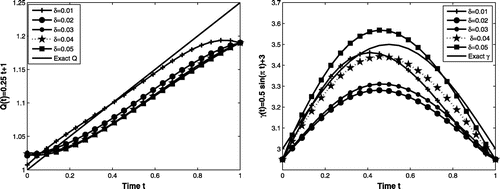
Figure 1. Exact and reconstruction $\mathit{\gamma }(t)$ (left) and Q(t) (right) using CGM and COMSOL for Example 6.1 for $\mathit{\varrho }=1\%$ noise in the data.

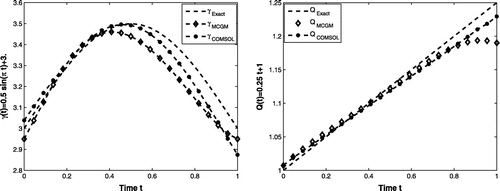
Figure 2. Exact and reconstructed $\mathit{\gamma }(t)$ (left) and Q(t) (right) using the modified CGM and COMSOL for Example 6.2 for $\mathit{\varrho }=1\%$ noise in the data.

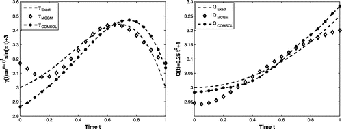
Figure 3. Exact and reconstructed $\mathit{\gamma }(t)$ (left) and Q(t) (right) using the modified CGM and COMSOL for Example 6.3 for $\mathit{\varrho }=1\%$ noise in the data.

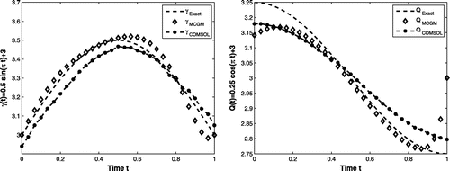
Figure 4. Convergence of the relative error of the reconstruction $\mathit{\gamma }$ and Q (left) and the residual accuracy error of $\mathit{\gamma }$ and Q (right) by Algorithm 5.1 for Example 6.3 with the number of iterations k.

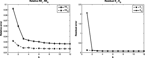
Figure 5. Exact and numerical reconstruction of heat flux (left) and Robin coefficient (right) by Algorithm 5.1 for Example 6.1 for various levels of noise $\mathit{\varrho }$ in the data.

Remark 6.1:

The relative error of the Robin coefficient is given by $\mathcal{R}{E}_{\mathit{\gamma }}=\frac{\Vert {\mathit{\gamma }}^k{-\mathit{\gamma }\Vert }_{L^2(0,\tilde{t})}}{{\Vert \mathit{\gamma }\Vert }_{L^2(0,\tilde{t})}}$ and the residual error with respect to $\mathit{\gamma }$ is given by $E_{\mathit{\gamma }}={\Vert T({\mathit{\gamma }}^k,Q^{k+1})-z^{\mathit{\delta }}\Vert }_{L^2(0,\tilde{t};L^2({\mathrm{\Gamma }}_c))}^2$. The relative error of the heat flux is given by $\mathcal{R}{E}_Q=\frac{\Vert Q^k{-Q\Vert }_{L^2(0,\tilde{t})}}{{\Vert Q\Vert }_{L^2(0,\tilde{t})}}$ and the residual error with respect to Q is given by $E_Q={\Vert T({\mathit{\gamma }}^k,Q^k)-z^{\mathit{\delta }}\Vert }_{L^2(0,\tilde{t};L^2({\mathrm{\Gamma }}_c))}^2$.

 

Table 1. The numerical results with respect to $\mathit{\gamma }$ and Q for $\mathit{\varrho }=1\%$ noise in the data using the modified CGM.

Example	$\mathrm{\Delta }t$	k	$\mathcal{R}{E}_{\mathit{\gamma }}$	$\mathcal{R}{E}_Q$	$({\mathit{\gamma }}^0,Q^0)$	Elapsed time in seconds
6.1	1/22	11	0.0264	0.0171	(3, 1.2)	9.36
6.2	1/20	11	0.0201	0.0102	(3.2, 3.2)	19.27
6.3	1/30	10	0.0112	0.0211	(3, 3)	22.30

Table 2. The numerical results with respect to $\mathit{\gamma }$ and Q for $\mathit{\varrho }=1\%$ noise in the data using COMSOL.

Example	$\mathrm{\Delta }t$	k	$\mathcal{R}{E}_{\mathit{\gamma }}$	$\mathcal{R}{E}_Q$	$({\mathit{\gamma }}^0,Q^0)$	Elapsed time in seconds
6.1	1/22	59	0.0184	0.0097	(3, 1.2)	64.33
6.2	1/20	51	0.0280	0.0063	(3.2, 3.2)	52.32
6.3	1/30	73	0.0153	0.0158	(3, 3)	75.35

Table 3. The numerical results (accuracy error) for Example 6.1 for various levels of noise $\mathit{\varrho }$.

$\mathcal{R}{E}_{\mathit{\gamma }}$	$\mathcal{R}{E}_Q$	$\mathit{\varrho }$	k	$J(\mathit{\gamma },Q)$
0.0401	0.0240	0	10	0.0088
0.0264	0.0171	$1\%$	11	0.0386
0.0508	0.0269	$2\%$	7	0.1512
0.0440	0.0318	$3\%$	6	0.3191
0.0180	0.0321	$4\%$	6	0.5389
0.0160	0.0329	$5\%$	6	0.8206

Figures 1–3 show the exact and reconstructed Robin coefficient and heat flux. Tables 1 and 2 show the numerical results for $\mathit{\gamma }(t)$ and Q(t) for $\mathit{\varrho }=1\%$ noise in the data using the modified CGM and COMSOL, respectively. From Tables 1 and 2, we can see that the elapsed time in case of modified CGM is less than the elapsed time of COMSOL under the same conditions. In addition, the mesh size for the three examples are not same.

The convergence of the Algorithm 5.1 proves to be steady for all examples. Figure 4 (left) shows the accuracy errors for the parameters $\mathit{\gamma }(t)$ and Q(t), while Figure 4 (right) shows the residual errors $E_{\mathit{\gamma }}$ and $E_Q$ which appear reasonable with the number of iterations. Also, the relative errors $\mathcal{R}{E}_{\mathit{\gamma }}$ and $\mathcal{R}{E}_Q$ indicate the efficiency and accuracy of the proposed Algorithm 5.1 (Figure 5 and Table 3). The minimum/optimal values are obtained after few iterations, this shows the rapidity of the proposed algorithm which is one of the main advantages of the modified CGM.

7. Summary and conclusions

In this paper, we have considered the problem of simultaneously reconstructing the heat flux and Robin coefficient in the heat conduction system from noisy measurements of the temperature on a single part of the boundary ${\mathrm{\Gamma }}_c$ over $t\in (0,\tilde{t})$. The Tikhonov regularization method was adopted to cope with the uncontrollable effect of the noise in the data. We have investigated the partial Fréchet derivatives of the forward solution to obtain the gradient of the Robin coefficient and heat flux. Furthermore, we have introduced the adjoint equations and obtained explicit expressions for simplifying step lengths calculation. The numerical algorithm was then investigated using the modified CGM. Afterwards, we have verified the robustness of the proposed algorithm against the noise. Furthermore, to verify the efficiency of the proposed algorithm we have compared the numerical results of the proposed method with the results obtained from the well-known finite-element software COMSOL Multiphysics under the same conditions. The proposed method has obtained stable numerical results for reconstructing the heat flux and Robin coefficient for various levels of noise.

Acknowledgements

The authors would like to thank the anonymous referees for their many constructive and insightful comments and suggestions, which have helped us improve the quality of the paper significantly.

Additional information

Funding

The work of Talaat Abdelhamid and Daijun Jiang was supported by National Natural Science Foundation of China [grant number 11401241], [grant number 11571265]; Daijun Jiang was supported by NSFC-RGC [China-Hong Kong number 11661161017].

Notes

No potential conflict of interest was reported by the authors.

References

- Hào DN , Thanh PX , Lesnic D . Determination of the heat transfer coefficients in transient heat conduction. Inverse Probl. 2013;29(9):095020.
- Hào DN , Thanh PX , Lesnic D . Determination of the ambient temperature in transient heat conduction. IMA J Appl Math. 2015;80:24–46.
- Martin T , Dulikravich G . Inverse determination of steady heat convection coefficient distributions. J Heat Transfer. 1998;120(2):328–334.
- Hào DN , Huong BV , Thanh PX , et al . Identification of nonlinear heat transfer laws from boundary observations. Appl Anal. 2015;94:1784–1799.
- Wikström P , Blasiak W , Berntsson F . Estimation of the transient surface temperature and heat flux of a steel slab using an inverse method. Appl Therm Eng. 2007;27(14):2463–2472.
- Beck JV , Blackwell B , Clair Jr. CRS . Inverse heat conduction: ill-posed problems. New York (NY): John Wiley and Sons; 1985.
- Kim SK , Lee WI . A maximum entropy solution for a two-dimensional inverse heat conduction problem. J Heat Transfer. 2003;125(6):1197–1205.
- Alifanov OM . Inverse heat transfer problems. Berlin: Springer-Verlag; 1994.
- Cattani L , Maillet D , Bozzoli F , et al . Estimation of the local convective heat transfer coefficient in pipe flow using a 2D thermal quadrupole model and truncated singular value decomposition. Int J Heat Mass Transfer. 2015;91:1034–1045.
- Kanzow C , Fukushima M , Yamashita N . Levenberg-Marquardt methods for constrained nonlinear equations with strong local convergence properties. Technique Report. Department of Applied Mathematics and Physics, Kyoto University; April, 2002.
- Yamashita N , Fukushima M . On the rate of convergence of the Levenberg-Marquardt method. In: Alefeld G , Chen X , editors. Topics in numerical analysis. Vol. 15, Computing Supplementa. Springer-Verlag; 2001. p. 239–249.
- Jin B , Zou J . Numerical estimation of the Robin coefficient in a stationary diffusion equation. IMA J Numer Anal. 2010;30(3):677–701.
- Cahlon B , Schochetman I , Shillor M . Convective cooling and optimal placement of electronic components with variable ambient temperature I. The linear model. J Comput Appl Math. 1993;47(3):351–367.
- Onyango T , Ingham DB , Lesnic D , et al . Determination of a time-dependent heat transfer coefficient from non-standard boundary measurements. Math Comput Simul. 2009;79(5):1577–1584.
- Slodicka M , Lesnic D , Onyango T . Determination of a time-dependent heat transfer coefficient in a nonlinear inverse heat conduction problem. Inverse Probl Sci Eng. 2010;18(1):65–81.
- Ditchfield C , Tadini CC , Singh R , et al . Velocity and temperature profiles, heat transfer coefficients and residence time distribution of a temperature dependent Herschel-Bulkley fluid in a tubular heat exchanger. J Food Eng. 2006;76(4):632–638.
- Alimoradi A , Veysi F . Prediction of heat transfer coefficients of shell and coiled tube heat exchangers using numerical method and experimental validation. Int J Therm Sci. 2016;107:196–208.
- Muraka P , Barrow G , Hinduja S . Influence of the process variables on the temperature distribution in orthogonal machining using the finite element method. Int J Mech Sci. 1979;21(8):445–456.
- Pacheco CC , Orlande HR , Colaco MJ , et al . Real-time identification of a high-magnitude boundary heat flux on a plate. Inverse Probl Sci Eng. 2016;24(9):1661–1679.
- Manual C . Comsol multiphysics user’s guide. Version 3; 2005. p. 1–622.
- Cardiff M , Kitanidis PK . Efficient solution of nonlinear, underdetermined inverse problems with a generalized PDE model. Comput Geosci. 2008;34(11):1480–1491.
- Brito R , Carvalho S , Silva SLE . Experimental investigation of thermal aspects in a cutting tool using comsol and inverse problem. Appl Therm Eng. 2015;86:60–68.
- Sousa J , Villafane L , Lavagnoli S , Paniagua G . Inverse heat flux evaluation using conjugate gradient methods from infrared imaging. In: 11th International Conference on Quantitative Infrared Thermography. Naples, Italy; 2012.
- Li R , Fang L , Deng Y , et al . Multi-parameter inverse analysis research based on Comsol Multiphysics and Matlab. In: 2010 International Conference on Computer Design and Applications (ICCDA). Vol. 2. IEEE, V2–164; 2010.
- Onyango TT , Ingham DB , Lesnic D . Restoring boundary conditions in heat conduction. J Eng Math. 2008;62(1):85–101.
- Onyango T , Ingham DB , Lesnic D . Reconstruction of heat transfer coefficients using the boundary element method. Comput Math Appl. 2008;56(1):114–126.
- Jin B , Lu X . Numerical identification of a Robin coefficient in parabolic problems. Math Comput. 2012;81(279):1369–1398.
- Cui M , Yang K , Xu X-L , et al . A modified Levenberg-Marquardt algorithm for simultaneous estimation of multi-parameters of boundary heat flux by solving transient nonlinear inverse heat conduction problems. Int J Heat Mass Transfer. 2016;97:908–916.
- Jiang D , Talaat TA . Simultaneous identification of Robin coefficient and heat flux in an elliptic system. Int J Comput Math. 2017;94(1):185–196.
- Abdelhamid T . Simultaneous identification of the spatio-temporal dependent heat transfer coefficient and spatially dependent heat flux using an MCGM in a parabolic system. J Comput Appl Math. 2018;27(328):164–176.
- Abdelhamid T , Deng X , Chen R . A new method for simultaneously reconstructing the space-time dependent Robin coefficient and heat flux in a parabolic system. Int J Numer Anal Model. 2017;14(6):893–915.
- Chrysafinos K , Gunzburger MD , Hou LS . Semidiscrete approximations of optimal Robin boundary control problems constrained by semilinear parabolic PDE. J Math Anal Appl. 2006;323(2):891–912.
- Reuther JJ , Jameson A , Alonso JJ , et al . Constrained multipoint aerodynamic shape optimization using an adjoint formulation and parallel computers, part 1. J Aircraft. 1999;36(1):51–60.
- Plessix R-E . A review of the adjoint-state method for computing the gradient of a functional with geophysical applications. Geophys J Int. 2006;167(2):495–503.
- Alifanov OM . Solution of an inverse problem of heat conduction by iteration methods. J Eng Phys Thermophys. 1974;26(4):471–476.
- Hansen P , O’Leary D . The use of the L-curve in the regularization of discrete ill-posed problems. SIAM J Sci Comput. 1993;14(6):1487–1503.
- Stanimirovic IP , Zlatanovic ML , Petkovic MD . On the linear weighted sum method for multi-objective optimization. Facta Acta Univ. 2011;26(4):49–63.
- Chowdhury S , Dulikravich GS . Improvements to single-objective constrained predator-prey evolutionary optimization algorithm. Struct Multidiscipl Optim. 2010;41(4):541–554.
- Powell MJD . The BOBYQA algorithm for bound constrained optimization without derivatives. Cambridge: University of Cambridge; 2009. p. 1–39. (Cambridge NA Report NA2009/06).