 ?Mathematical formulae have been encoded as MathML and are displayed in this HTML version using MathJax in order to improve their display. Uncheck the box to turn MathJax off. This feature requires Javascript. Click on a formula to zoom.
ABSTRACT
This paper deals with the determination of an initial condition in degenerate hyperbolic equation from final observations. With the aim of reducing the execution time, this inverse problem is solved using an approach based on double regularization: a Tikhonov’s regularization and regularization in equation by viscose-elasticity. So, we obtain a sequence of weak solutions of degenerate linear viscose-elastic problems. Firstly, we prove the existence and uniqueness of each term of this sequence. Secondly, we prove the convergence of this sequence to the weak solution of the initial problem. Also we present some numerical experiments to show the performance of this approach.
1. Introduction and main results
The inverse problems of finding unknown coefficients of a PDE from the partial knowledge of the system in a limited time interval are of interest in many applications: cosmology [Citation1], medicine [Citation2], in data assimilation [Citation3], it is used for the numerical weather forecast, ocean circulation, environmental prediction, geophysics [Citation4], remote sensing [Citation5] and many other areas.
Recently such type of problems received much attention, in particular, in degenerate parabolic and hyperbolic equations. Indeed, many problems coming from physics (models of Kolmogorov type in [Citation6], boundary layer models in [Citation7], . . . ), economics (Black-Merton-Scholes equations in [Citation8]) and biology (Fleming-Viot models in [Citation9] and Wright-Fisher models in [Citation10]) are described by degenerate parabolic or hyperbolic equations [Citation11]. This work is the continuity of [Citation12] and [Citation13], in which we identify the initial condition and we study numerically the null controllability of degenerate/singular parabolic problem. In this paper, we are interested in the estimation of the initial state of the degenerate hyperbolic problem (Equation1.1(1.1)
(1.1) ) below, thanks to a final observations
. The resolution of this inverse problem using only the Tikhonov’s regularization takes a considerable time of execution, to reduce it, we propose a new approach based on double regularization: the Tikhonov’s regularization and regularization in equation by viscose-elasticity.
Consider the degenerate hyperbolic equation(1.1)
(1.1)
where, ,
, and
.
Let a discritization of [0, T] with
,
is the step in time, and
.
We suppose that the observation of
is known in some points in vicinity of T:
such that
is known in
, with
.
The problem can be stated as follows:(1.2)
(1.2)
where the cost function E is defined as follows(1.3)
(1.3)
Subject to being the weak solution of the hyperbolic problem (Equation1.1
(1.1)
(1.1) ), with initial state u. The space
is the set of admissible initial states (will be defined later).
To solve this inverse problem, we propose an approach based on double regularization. The first is a regularization by viscose-elasticity, this gives the following degenerate linear viscose-elastic problem(1.4)
(1.4)
The second, is Tikhonov’s regularization. Since the problem (Equation1.2(1.2)
(1.2) ) is ill-posed in the sense of Hadamard, some regularization technique is needed in order to guarantee numerical stability of the computational procedure even with noisy input data. The problem thus consists in minimizing a functional of the form
(1.5)
(1.5)
subject to is the weak solution of the problem (Equation1.4
(1.4)
(1.4) ) with initial state u.
Here, the last term in (Equation1.5(1.5)
(1.5) ) stands for the so
called Tikhonov-type regularization ([Citation14,Citation15]),
being a small regularizing coefficient that provides extra convexity to the functional J.
an a priori (information) knowledge of the exact initial condition of the problem (Equation1.1
(1.1)
(1.1) ).
Firstly, we present a new theorem which gives the existence and uniqueness of the weak solutions of the problems (Equation1.4(1.4)
(1.4) ), for each
. Secondly, we prove that: when
, the sequence
of weak solutions of the problem (Equation1.4
(1.4)
(1.4) ) converges to the weak solution of the problem (Equation1.1
(1.1)
(1.1) ). Thirdly, with the aim of showing that the minimization problem and the direct problem are well-posed, we prove that the solution’s behaviour changes continuously with the initial conditions, for this we prove the continuity of the function
, where
is the weak solution of (Equation1.4
(1.4)
(1.4) ) with initial state
. Finally, we prove the differentiability of the functional J, which gives the existence of the gradient of J, that is computed using the adjoint state method. Also we present some numerical experiments to show the performance of this approach.
We now specify some notations. Let us introduce the functional spaces (see [Citation16–Citation18])
with the inner product
The weak formulation of the problem (Equation1.4(1.4)
(1.4) ) is:
(1.6)
(1.6)
Let(1.7)
(1.7)
We have the following results
Theorem 1.1:
[Citation19]]For any and
there exists a unique weak solution which solves the problem (Equation1.1
(1.1)
(1.1) ) such that
Moreover, there exists a constant such that for any solution of (Equation1.1
(1.1)
(1.1) )
(1.8)
(1.8)
Theorem 1.2:
Let a bounded regular open of
. We assume that
and
then the problem (Equation1.4
(1.4)
(1.4) ) has a unique weak solution such that
(1.9)
(1.9)
and we have the estimate(1.10)
(1.10)
The constant C depending on , and T.
Theorem 1.3:
When , the sequence of the weak solutions of the problem (Equation1.4
(1.4)
(1.4) ) converges to the weak solution of the problem (Equation1.1
(1.1)
(1.1) ).
Theorem 1.4:
Under the assumptions of Theorem 1.2, the functional J is continuous on .
Theorem 1.5:
Under the assumptions of Theorem 1.2, the functional J is G-derivable on .
2. Proof
Proof of Theorem 1.2:
For any positive integer n, consider the nondegenerate wave equation(2.1)
(2.1)
By the classical theory of wave equations, the system (Equation2.1(2.1)
(2.1) ) admits a unique classical solution
. Multiplying both sides of the first equation of (Equation2.1
(2.1)
(2.1) ) by
and integrating it in
, we have that
(2.2)
(2.2)
is independent of t, and by green’s formula, we arrive at
(2.3)
(2.3)
Integrating between 0 and t, with , gives
(2.4)
(2.4)
We have , and
, then
(2.5)
(2.5)
We pose(2.6)
(2.6)
Therefore(2.7)
(2.7)
We have(2.8)
(2.8)
then(2.9)
(2.9)
By Hölder inequality, we arrive at(2.10)
(2.10)
then(2.11)
(2.11)
In addition we have from where
(2.12)
(2.12)
From (Equation2.9(2.9)
(2.9) ), (Equation2.11
(2.11)
(2.11) ) and (Equation2.12
(2.12)
(2.12) ), we arrive at
(2.13)
(2.13)
Let(2.14)
(2.14)
and(2.15)
(2.15)
From (Equation2.7(2.7)
(2.7) ) and (Equation2.13
(2.13)
(2.13) ), we arrive at
(2.16)
(2.16)
Gronwall’s Lemma gives(2.17)
(2.17)
Let , which gives
(2.18)
(2.18)
Hence,(2.19)
(2.19)
and there exist a subsequence of
and a function
satisfying
, such that as
(2.20)
(2.20)
Since is the solution of system (Equation2.1
(2.1)
(2.1) ), we have that
and
.
Return to Equation (Equation2.3(2.3)
(2.3) ), by integrating between 0 and T, we obtain
(2.21)
(2.21)
From where(2.22)
(2.22)
From (Equation2.18(2.18)
(2.18) ), we obtain
(2.23)
(2.23)
and(2.24)
(2.24)
Then(2.25)
(2.25)
Consequently,(2.26)
(2.26)
The weak formulation of (Equation2.1(2.1)
(2.1) ) is
(2.27)
(2.27)
If we take as
, we obtain
(2.28)
(2.28)
(2.29)
(2.29)
From (Equation2.18(2.18)
(2.18) ) and (Equation2.25
(2.25)
(2.25) ), we obtain
(2.30)
(2.30)
Hence,(2.31)
(2.31)
We conclude that(2.32)
(2.32)
We find upon passing to weak limits that(2.33)
(2.33)
We obtain that is the weak solution of
(2.34)
(2.34)
Next, we prove the existence of weak solutions of (Equation1.4(1.4)
(1.4) ) for any
and
. Let
,
and
be Cauchy sequences of smooth functions, respectively, such that as
,
in
,
in
and
in
.
Denote by the solution of (Equation1.4
(1.4)
(1.4) ) associated to
and
, and
the solution of (Equation1.4
(1.4)
(1.4) ) associated to
and
.
We have the following variational problem(2.35)
(2.35)
Similarly at Equations (Equation2.18(2.18)
(2.18) ) and (Equation2.19
(2.19)
(2.19) ), let
and
We obtain(2.36)
(2.36)
and(2.37)
(2.37)
and(2.38)
(2.38)
Therefore, there exists and
, such that as
(2.39)
(2.39)
Now, we prove that the weak solution of problem (Equation1.4(1.4)
(1.4) ) is unique.
Let and
two weak solutions of the problem (Equation1.4
(1.4)
(1.4) ).
Let , consequently
verifies
(2.40)
(2.40)
By same way to obtain Equation (Equation2.18(2.18)
(2.18) ), we get
(2.41)
(2.41)
From where
Proof of Theorem 1.3:
Let the problem(2.42)
(2.42)
Multiplying both sides of the first equation of (Equation2.42(2.42)
(2.42) ) by
and integrating it in
, we have that
(2.43)
(2.43)
is independent of t, and by green’s formula, we arrive at
(2.44)
(2.44)
Integrating between 0 and t, with , gives
(2.45)
(2.45)
We pose(2.46)
(2.46)
Therefore we have(2.47)
(2.47)
We have(2.48)
(2.48)
By the same way as that used to obtain (Equation2.8(2.8)
(2.8) )–(Equation2.13
(2.13)
(2.13) ), we arrive at
(2.49)
(2.49)
Let , and
(2.50)
(2.50)
From (Equation2.47(2.47)
(2.47) ) and (Equation2.49
(2.49)
(2.49) ), we arrive at
(2.51)
(2.51)
Gronwall’s Lemma gives(2.52)
(2.52)
Let , which gives
(2.53)
(2.53)
Hence,(2.54)
(2.54)
and(2.55)
(2.55)
and(2.56)
(2.56)
Return to Equation (Equation2.44(2.44)
(2.44) ), by integrating between 0 and T we obtain
(2.57)
(2.57)
From where(2.58)
(2.58)
Since then
(2.59)
(2.59)
From where(2.60)
(2.60)
From Equation (Equation2.53(2.53)
(2.53) )
(2.61)
(2.61)
Consequently,(2.62)
(2.62)
The weak formulation of (Equation2.42(2.42)
(2.42) ) is
(2.63)
(2.63)
We take as
, we obtain
(2.64)
(2.64)
Since
, then
(2.65)
(2.65)
From Equations (Equation2.53(2.53)
(2.53) ) and (Equation2.61
(2.61)
(2.61) ), we have
(2.66)
(2.66)
Hence,(2.67)
(2.67)
We find upon passing to weak limits that(2.68)
(2.68)
Hence, is the weak solution of the problem (Equation1.1
(1.1)
(1.1) ).
Proof of Theorem 1.4:
The continuity of the functional J is deduced from the continuity of the function
We have the following lemma
Lemma 2.1:
Let the weak solution of (Equation1.4
(1.4)
(1.4) ) with initial state
. The function
(2.69)
(2.69)
is continuous.
Proof of Lemma 2.1:
Let a small variation such that
Consider , with
is the weak solution of (Equation1.4
(1.4)
(1.4) ) with initial state (
,
) and
is the weak solution of (Equation1.4
(1.4)
(1.4) ) with initial state
Consequently,
is the solution of the following variational problem
(2.70)
(2.70)
Hence, is weak solution of (Equation1.4
(1.4)
(1.4) ) with
. We apply the estimate in Theorem 1.2, we obtain
(2.71)
(2.71)
From where,(2.72)
(2.72)
and(2.73)
(2.73)
Which implies the continuity of the function(2.74)
(2.74)
Hence, the cost function J is continuous on .
Proof of Theorem 1.5:
The differentiability of the functional J is deduced from the differentiability of the function
where is the weak solution of the problem (Equation1.4
(1.4)
(1.4) ) with initial condition
. We have the following result
Lemma 2.2:
Let the weak solution of (Equation1.4
(1.4)
(1.4) ) with initial state
. The function
(2.75)
(2.75)
is G-derivable.
Proof of Lemma 2.2:
Let and
a small variation such that
, we define the function
(2.76)
(2.76)
where is the solution of the following variational problem
(2.77)
(2.77)
We pose(2.78)
(2.78)
We want to show that(2.79)
(2.79)
We easily verify that the function is solution of following variational problem
(2.80)
(2.80)
By the same way as that used in the proof of continuity, we deduce(2.81)
(2.81)
and(2.82)
(2.82)
Hence, The function is G-derivable, and we deduce that J is G-derivable on
.
Now, we compute the gradient of J using the adjoint state method.
3. Adjoint state method
We define the Gâteaux derivative of at
in the direction
, by
(3.1)
(3.1)
is the solution of (Equation1.4
(1.4)
(1.4) ) with initial state
and
is the solution of (Equation1.4
(1.4)
(1.4) ) with initial state k.
We compute the Gâteaux (directional) derivative of (Equation1.4(1.4)
(1.4) ) at k in some direction
and we get the so-called tangent linear model
(3.2)
(3.2)
We introduce the adjoint variable P, and we integrate(3.3)
(3.3)
We have(3.4)
(3.4)
We pose , then we obtain
(3.5)
(3.5)
Since
, then
.
From where(3.6)
(3.6)
Since
, then
and
. In addition, we have
. which gives
(3.7)
(3.7)
Based on the calculations done in the previous paragraph, we have(3.8)
(3.8)
This gives(3.9)
(3.9)
The discretization in time of (Equation3.9(3.9)
(3.9) ), using the Rectangular integration method, gives
(3.10)
(3.10)
We pose , the Gâteaux derivative of the cost function
at in the direction
is given by
After some compute, we arrive at(3.11)
(3.11)
The adjoint problem is(3.12)
(3.12)
The problem (Equation3.12(3.12)
(3.12) ) is retrograde, we make the change of variable
, the gradient of J becomes
(3.13)
(3.13)
To calculate a gradient of J, we solve two problems: direct problem (Equation1.4(1.4)
(1.4) ), and the adjoint problem (Equation3.12
(3.12)
(3.12) ) with the change of variable
.
4. Discretization of problem
Step 1. Full discretization
Discrete approximations of these problems need to be made for numerical implementation. To resolve the direct problem and the adjoint problem, we use the Method -schema in time. This method is unconditionally stable for
Let h the step in space and the step in time.
Let with
with
Let ,
,
and
(4.1)
(4.1)
We have(4.2)
(4.2)
(4.3)
(4.3)
with back affine approximation of in
we get
(4.4)
(4.4)
(4.5)
(4.5)
this gives(4.6)
(4.6)
the same, with back affine approximation of in
we get
(4.7)
(4.7)
From where(4.8)
(4.8)
(4.9)
(4.9)
Let(4.10)
(4.10)
and We have
Hence, is approximated by
(4.11)
(4.11)
where(4.12)
(4.12)
(4.13)
(4.13)
(4.14)
(4.14)
(4.15)
(4.15)
(4.16)
(4.16)
(4.17)
(4.17)
(4.18)
(4.18)
(4.19)
(4.19)
(4.20)
(4.20)
We have(4.21)
(4.21)
with we have
(4.22)
(4.22)
where(4.23)
(4.23)
(4.24)
(4.24)
We have , from where
and
Step 2. Discretization of the functional
(4.25)
(4.25)
We recall that the method of Thomas Simpson to calculate an integral is
with ,
,
,
.
Let the functions(4.26)
(4.26)
(4.27)
(4.27)
and(4.28)
(4.28)
We have
and
Let
This gives
From where
Therefore(4.29)
(4.29)
The main steps for descent method at each iteration are:
Calculate
solution of (Equation1.4
(1.4)
(1.4) ) with initial condition
,
Calculate
solution of adjoint problem,
Calculate the descent direction
,
Find
,
Update the variable
.
The value is chosen by the inaccurate linear search by Rule Armijo-Goldstein as following:
let
and
(for example
and
)
if
and stop
if not,
.
5. Numerical experiments
In this section, we do three tests:
In the first test, we show numerically that : when , the sequence
of weak solutions of the problem (Equation1.4
(1.4)
(1.4) ) converges to the weak solution of the problem (Equation1.1
(1.1)
(1.1) ). And we make a comparison between the proposed method and method based only on regularization Tikhonov.
In the second test, we study the impact of the percent of final knowledge () on the construction of the initial state.
In the third test, we study the noise resistance of the proposed method.
Remark: It is known in the literature that is very difficult to determine([Citation20,Citation21]). In order to choose
, we make each test for different values of
, and we choose the value of
which gives the best result.
We did all the tests on Pc with the following configurations: Intel Core i3 CPU 2.27GHz; We take step in space
and step in time
.
5.1. Convergence of the sequence 
 , when

the true state, and is the state to estimate.
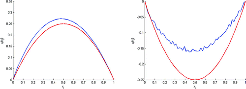
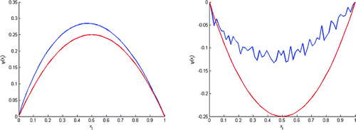
In figures below, the true initial state is drawn red, and rebuilt initial state of the problem (Equation1.4(1.4)
(1.4) ) in blue.
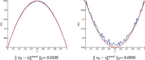
Figure 1. Test with . The value of
is not enough small, this figure shows that we can’t rebuild the solution.
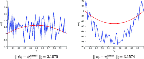
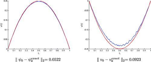
Figure 2. Test with . The value of
is not enough small, we can’t rebuild the true state. But the reconstructed initial condition starts to get near to the true state..
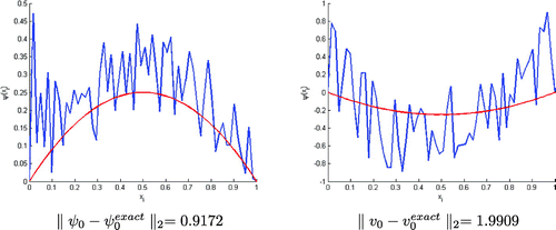
Table 1. Minimum value of J as function of . To get a better value of J, we must choose the value of
small enough.
Table shows the values of J obtained for different lambda value’s. These tests show numerically that when , the sequence
of weak solutions of the problem (Equation1.4
(1.4)
(1.4) ) converges to the weak solution of the problem (Equation1.1
(1.1)
(1.1) ) (Figures ). The rebuilt initial state begins to approach the true initial state as soon as
be lower than
(Figures and ).
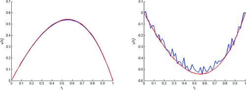
To validate this result, we did another test with , to construct the initial state
with
and
, we obtain the result follows
This test (Figure ) shows that we can rebuild the initial state with
. As the first test, we found that we can rebuild the initial state with
. And when
, the sequence
of weak solutions of the problem (Equation1.4
(1.4)
(1.4) ) converges to the weak solution of the problem (Equation1.1
(1.1)
(1.1) ).
In order to compare the proposed method based in double regularization with the Tikonov’s method, we did another test based only on tikhonov’s regularization, to reconstruct the initial state , with
The algorithm has found the solution with the minimum value of J equal to
in 72 h 54 min. Compared with the results in Table , we have a
of time gain with the double regularization method. This shows the effectiveness of this method to reduce the execution time to find the initial condition of the problem (Equation1.1
(1.1)
(1.1) ).
5.2. The impact of the percent of final knowledge 
 on the construction of the initial state
In these tests, we study the necessary percent of final knowledge of to estimate the initial state. In all tests we take
.
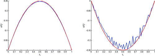
Figure 6. Test with of final knowledge of
. This figure shows that we can rebuild
(left) and
(right).
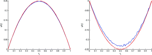
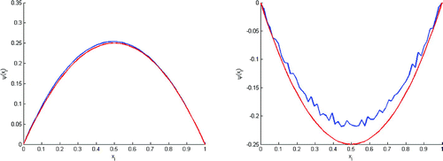
Figure 7. Test with of final knowledge of
. This figure shows that we can rebuild
(left) and
(right).
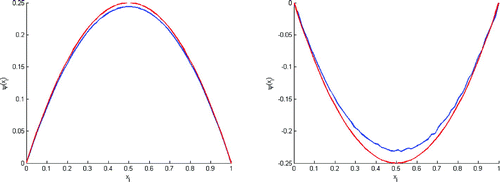
Figure 8. Test with of final knowledge of
. This figure shows that we can rebuild
(left) and
(right).
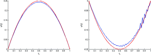
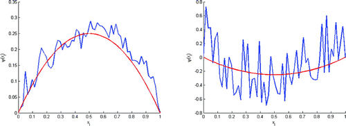
Figure 9. Test with of final knowledge of
. This figure shows that we can rebuild
(left), but we can’t rebuild
(right).
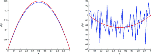
Figure 10. Test with of final knowledge of
. This figure shows that we can rebuild
(left), but we can’t rebuild
(right).
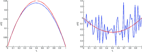
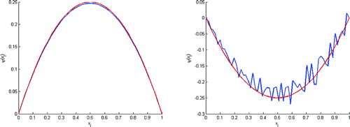
These tests show that we can rebuild with
of final knowledge of
(Figures ), but we lose
as soon as the percent of final knowledge be lower than
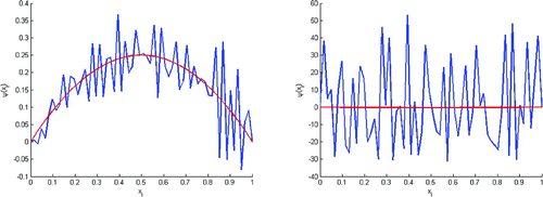
(Figures and ). Remark, The figure shows that we can’t rebuild the initial state in the case where
(Test without double regulation).
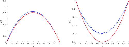
Figure 13. Test with . This figure shows that we can rebuild
(left), and
begins to move away from
,
(right).
5.3. The noise resistance of the proposed method
The data and
are assumed to be corrupted by measurement errors, which we will refer to as noise. In particular, we suppose that
and
. Let
and
. We consider that we have
of knowledge in final observation, we take
. And we did two tests:
In the first, we suppose , and we study the impact of err on the construction of the initial state. In the second test, we suppose
, and we study the impact of
on the construction of the initial state.
5.3.1. Impact of err on the construction of the initial state
These tests (Figures ) show that the proposed algorithm is uniformly stable to noise. And we can conclude that the tolerable percentage of err to rebuild the initial state is .
5.3.2. Impact of 
 on the construction of the initial state
These tests (Figures –) show that the proposed algorithm is uniformly stable to noise. And we can rebuild with
(Figures –), but we lose
as soon as
be superior than
(Figures –).
6. Conclusion
We have presented in this paper a new method based on double regularization applied to the determination of an initial state of hyperbolic degenerated problem from final observations. So, we have obtained a sequence of weak solutions of degenerate linear viscose-elastic problems. Firstly, we have proved the existence and uniqueness of each term of this sequence, and that this sequence converges to the weak solution of the initial problem. Secondly, we have proved that the solution’s behaviour changes continuously with the initial conditions. Also, in the numerical part, we have studied the noise resistance of the proposed method, and we have shown that this method proves effective to reduce the execution time.
Disclosure statement
No potential conflict of interest was reported by the authors.
References
- Frisch U , Matarrese S , Mohayaee R , Sobolevski A . A reconstruction of the initial conditions of the universe by optimal mass transportation. Nature. 2002;417(6886):260–262.
- Kuchment P , Kunyansky L . Mathematics of thermoacoustic tomography. Eur J Appl Math. 2008;19:191–224.
- Kalnay E . Atmospheric modeling, data assimilation and predictability. 2nd ed. New York (NY): Cam-bridge University Press; 2003.
- Gouveia WP , Scales JA . Bayesian seismic waveform inversion: parameter estimation and uncertainty analysis. J Geophys Res. 1998;103:2759–2779.
- Rodgers CD . Inverse methods for atmospheric sounding. London: World Scientific Press; 2000.
- Beauchard K , Zuazua E . Some controllability results for the 2D Kolmogorov equation. Ann Inst H Poincar Anal Non Linaire. 2009;26(5):1793–1815. DOI:10.1016/j.anihpc.2008.12.005. MR2566710 (2011b:93007).
- Buchot J-M , Raymond J-P . A linearized model for boundary layer equations, Optimal control of complex structures (Oberwolfach, 2000). International series of numerical mathematics. vol. 139. Birkhuser: Basel; 2002. p. 31–42. MR1901628 (2003g:35013).
- Emamirad H , Goldstein GR , Goldstein JA . Chaotic solution for the Black-Scholes equation. Proc Am Math Soc. 2012;140(6):2043–2052. DOI:10.1090/S0002-9939-2011-11069-4. MR2888192.
- Fleming WH , Viot M . Some measure-valued Markov processes in population genetics theory. Indiana Univ Math J. 1979;28(5):817–843. DOI:10.1512/iumj.1979.28.28058. MR542340 (81a:60059).
- Shimakura N . Partial differential operators of elliptic type, Translations of mathematical monographs. vol. 99. Providence (RI): American Mathematical Society; 1992. Translated and revised from the 1978 Japanese original by the author. MR1168472 (93h:35002).
- Fragnelli G , Mugnai D . Carleman estimates for singular parabolic equations with interior degeneracy and non smooth coefficients. Adv Nonlinear Anal. 2016. DOI:10.1515/anona-2015-0163.
- Atifi K , Essoufi E-H . Data assimilation and null controllability of degenerate/singular parabolic problems. Electron J Differ Equ. 2017;2017(135):1–17. ISSN: 1072-6691. Available from: http://ejde.math.txstate.edu or http://ejde.math.unt.edu
- Atifi K , Essoufi E-H , Khouiti B , et al . Identifying initial condition in degenerate parabolic equation with singular potential. Int J Differ Equ. 2017;17. DOI:10.1155/2017/1467049. Article ID 1467049.
- Bonnet M . Problmes inverses. Master recherche Ecole Centrale de Paris Mention Matire, Structures, Fluides, Rayonnement Spcialit Dynamique des Structures et Systmes Coupls, octobre 2008.
- Jens F . Generalized Tikhonov regularization. Basic theory and comprehensive results on convergence rates Dissertation, Fakultt fr Mathematik Technische Universitt Chemnitz, Oktober 2011.
- Alabau-Boussouira F , Cannarsa P , Fragnelli G . Carleman estimates for degenerate parabolic operators with applications to null controllability. J Evol Equ. 2006;6:161–204.
- Ait Ben Hassi EM , Ammar-Khodja F , Hajjaj A , et al . Carleman estimates and null controllability of degenerate parabolic systems. J Evol Equ Control Theory. 2013;2:441–459.
- Cannarsa P , Fragnelli G . null controllability of semilinear degenerate parabolic equations in bounded domains. Electron J Differ Equ. 2006;136:1–20.
- Zhang M , Gao H . Null controllability of some degenerate wave equations. Syst Sci Complex. 2016. DOI:10.1007/s11424-016-5281-3.
- Delbos F . Problmes d’optimisation Non Linaire avec Contraintes en Tomographie de Rflexion 3D. Thse. 2004.
- Hansen PC . Analysis of discrete ill-posed problems by mean of the Lcurve. SIAM Rev. 1992;34:561–580.

