Reconstruction for Sturm–Liouville equations with a constant delay with twin-dense nodal subsets

ABSTRACT

Inverse nodal problems for Sturm–Liouville equations with a constant delay are studied. The authors show that the potential up to its mean value on the whole interval can be uniquely determined by two twin-dense nodal subsets and present a constructive procedure for the solution of the above inverse nodal problem. Besides, an example shows that one twin-dense nodal subset can also reconstruct the potential up to its mean value on the whole interval for some cases, and a numerical example is presented.

KEYWORDS:

• Inverse nodal problem
• Sturm–Liouville equation
• a constant delay
• potential
• twin-dense nodal subset

2010 MATHEMATICS SUBJECT CLASSIFICATIONS:

• 34A55
• 34K29
• 45J05

1. Introduction

The following Sturm–Liouville equation with a constant delay is defined as follows: (1) $-u^{″}\left(x\right)+q\left(x\right)u(x-a)=\lambda u\left(x\right),0<x<\pi ,$(1) where $q\left(x\right)$ is a real-valued function and $q\in L^2[0,\pi ]$ and $q\left(x\right)\stackrel{a.e.}{=}0$ on $[0,a],0<a<\pi$. The presence of a delay in the mathematical model causes phenomena that essentially influence the entire process. Technological and constructive improvements for such models require taking into account such phenomena even in the classical areas of engineering (see [1] and references therein). Direct and inverse problems for differential operators with a constant delay were found in [2–6], some results on inverse problems for integro-differential operators (operators with integral delay) can be found in [7].

We shall denote the operator $L_{\xi }(q,a)$ with Equation (1(1) $-u^{″}\left(x\right)+q\left(x\right)u(x-a)=\lambda u\left(x\right),0<x<\pi ,$(1) ) and boundary conditions (2) $u\left(0\right)=0,u^{\left(\xi \right)}\left(\pi \right)=0,\mathrm{for}\xi =0,1.$(2)

The inverse spectral problem consists in recovering the operator from its spectral characteristics. Inverse spectral problems for the Sturm–Liouville operator have been studied fairly completely(see [8–12] and the references therein). Although there seems to be only a little difference between the Sturm–Liouville operator and the operator $L_{\xi }(q,a)$, some of the features are unlike (see [1,2,8]). For instance, the main methods in the inverse problem theory for the Sturm–Liouville operator (transformation operator method, method of spectral mappings, and others) do not give reliable results for differential operators with a constant delay.

The inverse nodal problem is to reconstruct this operator from the given nodal points (zeros) of its eigenfunctions. In 1988, McLaughlin [13] showed that a dense subset of nodal points of its eigenfunctions for the classical Sturm–Liouville operator is sufficient to determine the potential q up to its mean value and coefficients h,H of boundary conditions. After then, a number of researchers studied the inverse nodal problems for differential pencils, discontinuous Sturm–Liouville problems, the p-Laplacian, the transmission eigenvalue problem, Sturm–Liouville equations on graphs and so on (see [7,12,14–29] and references therein). In particular, X.F. Yang [28] showed that an s-dense nodal set on the interval $[0,b_0]$ for the classical Sturm–Liouville operator, $\frac{1}{2}<b_0\le 1$, is sufficient to determine the potential q up to its mean value by applying Gesztesy–Simon theorem [9]. Then, Cheng, Law and Tsay [15] improved the Yang's results by the twin-dense subset on $[0,b_0]$ (see below, Definition 3.2, or [15] and other works) instead of s-dense nodal set. Later, Guo and Wei [17] showed that the potential $q\left(x\right)$ up to its mean value can be uniquely determined by the twin-dense subset on $[a_0,b_0]$ for the case $a_0<\frac{1}{2}<b_0$. A counterexample in [27] illustrates that two Sturm–Liouville operators have the same spectrum and in the subinterval $[0,((1-\alpha )/2\left)\right]\bigcup \left[\right((1+\alpha )/2),1]$ for any $\alpha ,0<\alpha <1$, their nodal points are the same, but $q\left(x\right)\ne \tilde{q}\left(x\right)$ on the interval $\left(\right(1-\alpha )/2,(1+\alpha \left)/2\right)$. Later, Wang and Yurko [26] studied the inverse nodal problem for discontinuous Sturm–Liouville problems by the twin-dense subset on $[a_0,b_0]$. Inverse problems are more difficult for investigation of Equation (1(1) $-u^{″}\left(x\right)+q\left(x\right)u(x-a)=\lambda u\left(x\right),0<x<\pi ,$(1) ) –Equation (2(2) $u\left(0\right)=0,u^{\left(\xi \right)}\left(\pi \right)=0,\mathrm{for}\xi =0,1.$(2) ) with the spectral data, and nowadays in this direction there are only a number of results (see [2–4] and other works) which do not constitute a general picture. The aims of this paper are to study the inverse nodal problems for the Sturm–Liouville operator with a constant delay.

This article is organized as follows. In Section 2, we present preliminaries. The inverse nodal problems for Sturm–Liouville equations with a constant delay are studied in Section 3.

2. Preliminaries

Let $S(x,\rho )$ be the solution of the Equation (1(1) $-u^{″}\left(x\right)+q\left(x\right)u(x-a)=\lambda u\left(x\right),0<x<\pi ,$(1) ) associated with initial conditions $S(0,\rho )=0$ and $S^{\prime }(0,\rho )=1$. Denote $\lambda ={\rho }^2$ and $\tau =|\mathrm{Im}\rho |$. Then $S(x,\rho )$ and $S^{\prime }(x,\rho )$ satisfy (see [3]): (3) $\begin{array}{rl}S(x,\rho )& =\frac{\sin \left(\rho x\right)}{\rho }+{\int }_a^x\frac{\sin \rho (x-t)}{\rho }q\left(t\right)S(t-a,\lambda )\mathrm{d}t\\ & =\frac{\sin \left(\rho x\right)}{\rho }-\frac{\cos \rho (x-a)}{2{\rho }^2}{\int }_a^{x}q\left(t\right)\mathrm{d}t\\ & +\frac{1}{2{\rho }^2}{\int }_a^{x}q\left(t\right)\cos (x-2t+a)\mathrm{d}t+O\left(\frac{{\mathrm{e}}^{\tau x}}{{\rho }^3}\right),\end{array}$(3) (4) $\begin{array}{rl}{S}^{\prime }(x,\rho )& =\cos \left(\rho x\right)+\frac{\sin \left(\rho \right(x-a\left)\right)}{2\rho }{\int }_a^{x}q\left(t\right)\mathrm{d}t\\ & +\frac{1}{2\rho }{\int }_a^{x}q\left(t\right)\sin \left(\rho \right(x-2t+a\left)\right)\mathrm{d}t+O\left(\frac{{\mathrm{e}}^{\tau x}}{{\rho }^2}\right)\end{array}$(4) for sufficiently large λ, uniformly in $x\in [a,\pi ]$. Each eigenvalue of $L_{\xi }$ is real and simple, and the spectral set of $L_{\xi }$ coincides with the set of zero of its characteristic function (5) ${\mathrm{\Delta }}_{\xi }\left(\lambda \right):=S^{\left(\xi \right)}(\pi ,\lambda ).$(5) Denote ${\lambda }_{n,\xi }={\rho }_{n,\xi }^2,n\ge 1$. Then the eigenvalues ${\lambda }_{n,\xi }$ satisfy the following asymptotic formula (see [2,3]): (6) ${\rho }_{n,\xi }=\left(n-\frac{\xi }{2}\right)+\frac{\omega \cos \left(\left(n-\frac{\xi }{2}\right)a\right)}{n\pi }+\frac{{\kappa }_{n,\xi }}{n},$(6) where $\omega =\frac{1}{2}{\int }_a^{\pi }q\left(t\right)\mathrm{d}t$, $\left\{{\kappa }_{n,\xi }\right\}\in l^2$.

3. Inverse nodal problems

From now on, we denote ${\tilde{L}}_{\xi }=L_{\xi }(\tilde{q},a)$ which is of the same form as L but with different coefficients. If a certain symbol γ denotes an object related to $L_{\xi }$, then the corresponding symbol $\tilde{\gamma }$ denotes the analogous object related to ${\tilde{L}}_{\xi }$, and $\hat{\gamma }=\gamma -\tilde{\gamma }$. In this section, we shall show our main results of inverse nodal problems for the Sturm–Liouville equation with a constant delay. Since $q\left(x\right)\stackrel{a.e.}{=}0$ on $[0,a],$ we shall only concern with the nodal subset on $[a,\pi ]$. We have the following nodal formulae in $[a,\pi ]$ for $L_{\xi }(q,a)$.

Lemma 3.1

For $\xi =0,1,$ the zero $x_{n,\xi }^j$ of the eigenfunction $S(x,{\lambda }_{n,\xi })$ of $L_{\xi }(q,a)$ satisfy the following formula: (7) $x_{n,\xi }^j=\frac{j\pi }{n-\frac{\xi }{2}}+\cos \left(\left(n-\frac{\xi }{2}\right)a\right)\left(\frac{{\int }_0^{x_{n,\xi }^j}q\left(t\right)\mathrm{d}t}{2{\left(n-\frac{\xi }{2}\right)}^2}-\frac{j\omega }{{\left(n-\frac{\xi }{2}\right)}^3}\right)+o\left(\frac{1}{n^2}\right).$(7)

Proof.

By virtue of Equation (3(3) $\begin{array}{rl}S(x,\rho )& =\frac{\sin \left(\rho x\right)}{\rho }+{\int }_a^x\frac{\sin \rho (x-t)}{\rho }q\left(t\right)S(t-a,\lambda )\mathrm{d}t\\ & =\frac{\sin \left(\rho x\right)}{\rho }-\frac{\cos \rho (x-a)}{2{\rho }^2}{\int }_a^{x}q\left(t\right)\mathrm{d}t\\ & +\frac{1}{2{\rho }^2}{\int }_a^{x}q\left(t\right)\cos (x-2t+a)\mathrm{d}t+O\left(\frac{{\mathrm{e}}^{\tau x}}{{\rho }^3}\right),\end{array}$(3) ), $S(x,{\lambda }_{n,\xi })=\frac{\sin \left({\rho }_{n,\xi }x\right)}{{\rho }_{n,\xi }}-\frac{\cos \left({\rho }_{n,\xi }(x-a)\right)}{2{\left({\rho }_{n,\xi }\right)}^2}{\int }_a^{x}q\left(t\right)\mathrm{d}t+o\left(\frac{1}{n^2}\right).$ Since $S(x_{n,\xi }^j,{\lambda }_{n,\xi })=0$, we have $\begin{array}{rl}& \sin \left({\rho }_{n,\xi }{x}_{n,\xi }^j\right)-\frac{\cos \left({\rho }_{n,\xi }{x}_{n,\xi }^j\right)\cos \left({\rho }_{n,\xi }a\right)+\sin \left({\rho }_{n,\xi }{x}_{n,\xi }^j\right)\sin \left({\rho }_{n,\xi }a\right)}{2{\rho }_{n,\xi }}\\ & {\int }_a^{x_{n,\xi }^j}q\left(t\right)\mathrm{d}t+o\left(\frac{1}{n}\right)=0.\end{array}$ This implies (8) $\tan \left({\rho }_{n,\xi }{x}_{n,\xi }^j\right)=\frac{\cos \left(\left(n-\frac{\xi }{2}\right)a\right)}{2{\rho }_{n,\xi }}{\int }_a^{x_{n,\xi }^j}q\left(t\right)\mathrm{d}t+o\left(\frac{1}{n}\right).$(8) By using Taylor's expansions, then Equation (8(8) $\tan \left({\rho }_{n,\xi }{x}_{n,\xi }^j\right)=\frac{\cos \left(\left(n-\frac{\xi }{2}\right)a\right)}{2{\rho }_{n,\xi }}{\int }_a^{x_{n,\xi }^j}q\left(t\right)\mathrm{d}t+o\left(\frac{1}{n}\right).$(8) ) shows ${\rho }_{n,\xi }{x}_{n,\xi }^j=j\pi +\frac{\cos \left(\left(n-\frac{\xi }{2}\right)a\right)}{2{\rho }_{n,\xi }}{\int }_0^{x_{n,j}^j}q\left(t\right)\mathrm{d}t+o\left(\frac{1}{n}\right),$ as $n\to \mathrm{\infty }.$ This implies (9) $x_{n,\xi }^j=\frac{j\pi }{{\rho }_{n,\xi }}+\frac{\cos \left(\left(n-\frac{\xi }{2}\right)a\right)}{2{\rho }_{n,\xi }^2}{\int }_0^{x_{n,\xi }^j}q\left(t\right)\mathrm{d}t+o\left(\frac{1}{n^2}\right).$(9) By virtue of Equation (6(6) ${\rho }_{n,\xi }=\left(n-\frac{\xi }{2}\right)+\frac{\omega \cos \left(\left(n-\frac{\xi }{2}\right)a\right)}{n\pi }+\frac{{\kappa }_{n,\xi }}{n},$(6) ), we have the following asymptotic formulae (10) $\begin{array}{rl}\frac{1}{{\rho }_{n,\xi }}=& \frac{1}{\left(n-\frac{\xi }{2}\right)}-\frac{\omega \cos \left(\left(n-\frac{\xi }{2}\right)a\right)}{{\left(n-\frac{\xi }{2}\right)}^3\pi }+o\left(\frac{1}{n^3}\right),\end{array}$(10) (11) $\begin{array}{rl}\frac{1}{{\rho }_{n,\xi }^2}=& \frac{1}{{\left(n-\frac{\xi }{2}\right)}^2}+o\left(\frac{1}{n^2}\right).\end{array}$(11) Substituting Equations (10(10) $\begin{array}{rl}\frac{1}{{\rho }_{n,\xi }}=& \frac{1}{\left(n-\frac{\xi }{2}\right)}-\frac{\omega \cos \left(\left(n-\frac{\xi }{2}\right)a\right)}{{\left(n-\frac{\xi }{2}\right)}^3\pi }+o\left(\frac{1}{n^3}\right),\end{array}$(10) ) and (11(11) $\begin{array}{rl}\frac{1}{{\rho }_{n,\xi }^2}=& \frac{1}{{\left(n-\frac{\xi }{2}\right)}^2}+o\left(\frac{1}{n^2}\right).\end{array}$(11) ) into Equation (9(9) $x_{n,\xi }^j=\frac{j\pi }{{\rho }_{n,\xi }}+\frac{\cos \left(\left(n-\frac{\xi }{2}\right)a\right)}{2{\rho }_{n,\xi }^2}{\int }_0^{x_{n,\xi }^j}q\left(t\right)\mathrm{d}t+o\left(\frac{1}{n^2}\right).$(9) ), we obtain Equation (7(7) $x_{n,\xi }^j=\frac{j\pi }{n-\frac{\xi }{2}}+\cos \left(\left(n-\frac{\xi }{2}\right)a\right)\left(\frac{{\int }_0^{x_{n,\xi }^j}q\left(t\right)\mathrm{d}t}{2{\left(n-\frac{\xi }{2}\right)}^2}-\frac{j\omega }{{\left(n-\frac{\xi }{2}\right)}^3}\right)+o\left(\frac{1}{n^2}\right).$(7) ). Therefore, the proof of Lemma 3.1 is completed.

Denote $l_{n,\xi }^j:=x_{n,\xi }^{j+1}-x_{n,\xi }^j$, one can derive $l_{n,\xi }^j=\frac{\pi }{n-\frac{\xi }{2}}+O\left(\frac{1}{n^2}\right)$ from Lemma 3.1. Let $X_{\xi }:=\{x_{n,\xi }^j{\}}_{n,j\in \mathbb{N}}\cap [a,\pi ]$ be the set of nodal points of $L_{\xi }(q,a).$ Clearly $X_{\xi }$ is the dense set on $[a,\pi ]$. Define the function $j_{n,\xi }\left(x\right)$ on $(a,\pi )$ by $j_{n,\xi }\left(x\right):=max\{j:x_{n,\xi }^j\le x\},\xi =0,1.$ Therefore, for fixed $n,x,$ then there exists a $j_{n,\xi }\left(x\right)=j$ such that $x\in [x_{n,\xi }^j,x_{n,\xi }^{j+1})$.

Definition 3.2

Let $B:=\{n_k|n_k\in \mathbb{N}{\}}_{k=1}^{\mathrm{\infty }}$ be a strictly increasing sequence of natural numbers. For each $\xi =0,1$ We call $W_{B,\xi }\left(\right[a_0,b_0\left]\right)\subseteq [a_0,b_0],a\le a_0<b_0\le \pi$, be a twin-dense nodal subset on $[a_0,b_0]$ of $X_{\xi }$, if

1. $W_{B,\xi }\left(\right[a_0,b_0\left]\right)\subseteq X_{\xi }\bigcap [a_0,b_0]$.

2. For all $n_k\in B$, there exists $j_k$ such that both $x_{n_k,\xi }^{j_k},x_{n_k,\xi }^{j_k+1}\in W_{B,\xi }\left(\right[a_0,b_0\left]\right)$.

3. The set $W_{B,\xi }\left(\right[a_0,b_0\left]\right)$ is dense on $[a_0,b_0]$, i.e. $\overline{W_{B,\xi }\left(\right[a_0,b_0\left]\right)}=[a_0,b_0]$.

In this paper, we say $W_{B,\xi }\left(\right[a_0,b_0\left]\right)={\tilde{W}}_{\tilde{B},\xi }\left(\right[a_0,b_0\left]\right)$ if $x_{n_k,\xi }^{j_k+j}={\tilde{x}}_{{\tilde{n}}_k,\xi }^{{\tilde{j}}_k+j}$ for all $j\in \mathbb{N},$ where $x_{n_k,\xi }^{j_k+j}\in W_{B,\xi }\left(\right[a_0,b_0\left]\right)$ and ${\tilde{x}}_{{\tilde{n}}_k,\xi }^{{\tilde{j}}_k+j}\in {\tilde{W}}_{\tilde{B},\xi }\left(\right[a_0,b_0\left]\right).$ The following inverse nodal problem is what we concern:

Inverse Problem: Given two twin-dense nodal subsets $W_{B,\xi }\left(\right[a_0,b_0\left]\right)$, $\xi =0,1$, on the interval $[a_0,b_0]$, we reconstruct the potential $q\left(x\right)$.

The following results can solve the Inverse Problem completely.

Theorem 3.3

The potential $q\left(x\right)$ on $[a,\pi ]$ up to its mean value can be uniquely determined by the given twin-dense nodal subsets $W_{B,\xi }\left(\right[a,\pi \left]\right)$ for $\xi =0,1.$

Proof.

For each fixed $x\in [a,\pi ]$, we choose $x_{n_k,\xi }^{j_{n_k}}$ and $x_{n_k,\xi }^{j_{n_k}+1}\in W_{B,\xi }\left(\right[a,\pi \left]\right)$ such that $\underset{k\to \mathrm{\infty }}{lim}{x}_{n_k,\xi }^{j_{n_k}}=x$. From Equation (7(7) $x_{n,\xi }^j=\frac{j\pi }{n-\frac{\xi }{2}}+\cos \left(\left(n-\frac{\xi }{2}\right)a\right)\left(\frac{{\int }_0^{x_{n,\xi }^j}q\left(t\right)\mathrm{d}t}{2{\left(n-\frac{\xi }{2}\right)}^2}-\frac{j\omega }{{\left(n-\frac{\xi }{2}\right)}^3}\right)+o\left(\frac{1}{n^2}\right).$(7) ), we have $\underset{k\to \mathrm{\infty }}{lim}\frac{j_{n_k}\pi }{n-\frac{\xi }{2}}=x,\xi =0,1.$ Therefore, (12) $\begin{array}{rl}f\left(x\right)& :=\underset{k\to \mathrm{\infty }}{lim}2\left\{\sin \left(n_{k}a\right)\left[(n_k-\frac{1}{2}{)}^2{x}_{n_k,1}^{j_{n_k}}-(n_k-\frac{1}{2})j_{n_k}\pi \right]\right.\\ & -\left.\sin \left(\right(n_k-\frac{1}{2}\left)a\right)\left[n_k^2{x}_{n_k,0}^{j_{n_k}}-n_k{j}_{n_k}\pi \right]\right\}\\ & =\underset{k\to \mathrm{\infty }}{lim}\left[\sin \frac{a}{2}\left({\int }_a^{x_{n_k,\xi }^{j_{n_k}}}q\left(t\right)\mathrm{d}t-\frac{2j_{n_k}\omega }{n_k}\right)+o\left(1\right)\right]\\ & =\sin \frac{a}{2}\left({\int }_0^{x}q\left(t\right)\mathrm{d}t-\frac{x}{\pi }{\int }_a^{\pi }q\left(t\right)\mathrm{d}t\right),a>0.\end{array}$(12) By taking derivatives for Equation (12(12) $\begin{array}{rl}f\left(x\right)& :=\underset{k\to \mathrm{\infty }}{lim}2\left\{\sin \left(n_{k}a\right)\left[(n_k-\frac{1}{2}{)}^2{x}_{n_k,1}^{j_{n_k}}-(n_k-\frac{1}{2})j_{n_k}\pi \right]\right.\\ & -\left.\sin \left(\right(n_k-\frac{1}{2}\left)a\right)\left[n_k^2{x}_{n_k,0}^{j_{n_k}}-n_k{j}_{n_k}\pi \right]\right\}\\ & =\underset{k\to \mathrm{\infty }}{lim}\left[\sin \frac{a}{2}\left({\int }_a^{x_{n_k,\xi }^{j_{n_k}}}q\left(t\right)\mathrm{d}t-\frac{2j_{n_k}\omega }{n_k}\right)+o\left(1\right)\right]\\ & =\sin \frac{a}{2}\left({\int }_0^{x}q\left(t\right)\mathrm{d}t-\frac{x}{\pi }{\int }_a^{\pi }q\left(t\right)\mathrm{d}t\right),a>0.\end{array}$(12) ), we have (13) $q\left(x\right)-\frac{1}{\pi }{\int }_a^{\pi }q\left(t\right)\mathrm{d}t\stackrel{a.e.}{=}\frac{1}{\sin \frac{a}{2}}{f}^{\prime }\left(x\right),x\in [a,\pi ],a>0.$(13) Thus, the proof of Theorem 3.3 is completed.

The proof of Theorem 3.3 is constructive. Therefore, a constructive procedure for the solution of the Inverse Problem is presented as follows.

Algorithm: Given the twin-dense nodal subsets $W_{B,\xi }\left(\right[a,\pi \left]\right)$, $\xi =0,1$, reconstruct $q\left(x\right)$.

1. For each fixed $x\in [a,\pi ]$, we choose a sequence $\left\{x_{n_k,\xi }^{j_{n_k}}\right\}\subseteq W_{B,\xi }\left(\right[a,\pi \left]\right)$ such that $\underset{k\to \mathrm{\infty }}{lim}{x}_{n_k,\xi }^{j_{n_k}}=x$;

2. We calculate $f\left(x\right)$ by Equation (12(12) $\begin{array}{rl}f\left(x\right)& :=\underset{k\to \mathrm{\infty }}{lim}2\left\{\sin \left(n_{k}a\right)\left[(n_k-\frac{1}{2}{)}^2{x}_{n_k,1}^{j_{n_k}}-(n_k-\frac{1}{2})j_{n_k}\pi \right]\right.\\ & -\left.\sin \left(\right(n_k-\frac{1}{2}\left)a\right)\left[n_k^2{x}_{n_k,0}^{j_{n_k}}-n_k{j}_{n_k}\pi \right]\right\}\\ & =\underset{k\to \mathrm{\infty }}{lim}\left[\sin \frac{a}{2}\left({\int }_a^{x_{n_k,\xi }^{j_{n_k}}}q\left(t\right)\mathrm{d}t-\frac{2j_{n_k}\omega }{n_k}\right)+o\left(1\right)\right]\\ & =\sin \frac{a}{2}\left({\int }_0^{x}q\left(t\right)\mathrm{d}t-\frac{x}{\pi }{\int }_a^{\pi }q\left(t\right)\mathrm{d}t\right),a>0.\end{array}$(12) ).

3. By taking derivatives for Equation (12(12) $\begin{array}{rl}f\left(x\right)& :=\underset{k\to \mathrm{\infty }}{lim}2\left\{\sin \left(n_{k}a\right)\left[(n_k-\frac{1}{2}{)}^2{x}_{n_k,1}^{j_{n_k}}-(n_k-\frac{1}{2})j_{n_k}\pi \right]\right.\\ & -\left.\sin \left(\right(n_k-\frac{1}{2}\left)a\right)\left[n_k^2{x}_{n_k,0}^{j_{n_k}}-n_k{j}_{n_k}\pi \right]\right\}\\ & =\underset{k\to \mathrm{\infty }}{lim}\left[\sin \frac{a}{2}\left({\int }_a^{x_{n_k,\xi }^{j_{n_k}}}q\left(t\right)\mathrm{d}t-\frac{2j_{n_k}\omega }{n_k}\right)+o\left(1\right)\right]\\ & =\sin \frac{a}{2}\left({\int }_0^{x}q\left(t\right)\mathrm{d}t-\frac{x}{\pi }{\int }_a^{\pi }q\left(t\right)\mathrm{d}t\right),a>0.\end{array}$(12) ), we find the potential $q\left(x\right)$ satisfying $q\left(x\right)-\frac{1}{\pi }{\int }_a^{\pi }q\left(t\right)\mathrm{d}t\stackrel{a.e.}{=}\frac{1}{\sin \frac{a}{2}}{f}^{\prime }\left(x\right),x\in [a,\pi ].$

Remark 3.4

1. Since the limit $\underset{k\to \mathrm{\infty }}{lim}\cos \left(\left(n_k-\frac{\xi }{2}\right)a\right),\xi =0,1$ may not exist, or 0, we may not reconstruct the potential $q\left(x\right)$ on $[a,\pi ]$ by only one twin-dense nodal subset. In fact the condition ‘existence of the above limit’, or $\cos \left(\right(n_k-\left(\xi /2\right)\left)a\right)\ne 0$, is so crucial that Theorem 3.3 for one twin-dense nodal subset may be invalid for any a and B. However, only one twin-dense nodal subset can also reconstruct the potential $q\left(x\right)$ on $[a,\pi ]$ for some a and B (see below, Example 3.6).

2. Clearly Equation (13(13) $q\left(x\right)-\frac{1}{\pi }{\int }_a^{\pi }q\left(t\right)\mathrm{d}t\stackrel{a.e.}{=}\frac{1}{\sin \frac{a}{2}}{f}^{\prime }\left(x\right),x\in [a,\pi ],a>0.$(13) ) is violated for a=0. If a=0, then the Equation (1(1) $-u^{″}\left(x\right)+q\left(x\right)u(x-a)=\lambda u\left(x\right),0<x<\pi ,$(1) ) becomes the classical Sturm–Liouville equation. Therefore one can only reconstruct $q\left(x\right)$ from one twin-dense nodal subset (see [13] and other works).

By virtue of the above algorithm, we obtain the uniqueness theorem:

Theorem 3.5

If $W_{B,\xi }\left(\right[a,\pi \left]\right)={\tilde{W}}_{\tilde{B},\xi }\left(\right[a,\pi \left]\right)$ for $\xi =0,1,$ then (14) $q\left(x\right)-\frac{1}{\pi }{\int }_a^{\pi }q\left(t\right)\mathrm{d}t\stackrel{a.e.}{=}\tilde{q}\left(x\right)-\frac{1}{\pi }{\int }_a^{\pi }\tilde{q}\left(t\right)\mathrm{d}t\mathrm{on}[a,\pi ].$(14)

Proof.

For each fixed $x\in [a,\pi ]$, we choose $x_{n_k,\xi }^{j_{n_k}}\mathrm{and}{x}_{n_k,\xi }^{j_{n_k}+1}\in W_{B,\xi }\left(\right[a,\pi \left]\right)$ such that $\underset{k\to \mathrm{\infty }}{lim}{x}_{n_k,\xi }^{j_{n_k}}=x$. By virtue of (13(13) $q\left(x\right)-\frac{1}{\pi }{\int }_a^{\pi }q\left(t\right)\mathrm{d}t\stackrel{a.e.}{=}\frac{1}{\sin \frac{a}{2}}{f}^{\prime }\left(x\right),x\in [a,\pi ],a>0.$(13) ), we reconstruct $q\left(x\right)$ by $q\left(x\right)-\frac{1}{\pi }{\int }_a^{\pi }q\left(t\right)\mathrm{d}t\stackrel{a.e.}{=}\frac{1}{\sin \frac{a}{2}}{f}^{\prime }\left(x\right),x\in [a,\pi ],a>0.$ By virtue of the assumption $W_{B,\xi }\left(\right[a,\pi \left]\right)={\tilde{W}}_{\tilde{B},\xi }\left(\right[a,\pi \left]\right)$ of Theorem 3.5 together with the function $f\left(x\right)$ defined by Equation (12(12) $\begin{array}{rl}f\left(x\right)& :=\underset{k\to \mathrm{\infty }}{lim}2\left\{\sin \left(n_{k}a\right)\left[(n_k-\frac{1}{2}{)}^2{x}_{n_k,1}^{j_{n_k}}-(n_k-\frac{1}{2})j_{n_k}\pi \right]\right.\\ & -\left.\sin \left(\right(n_k-\frac{1}{2}\left)a\right)\left[n_k^2{x}_{n_k,0}^{j_{n_k}}-n_k{j}_{n_k}\pi \right]\right\}\\ & =\underset{k\to \mathrm{\infty }}{lim}\left[\sin \frac{a}{2}\left({\int }_a^{x_{n_k,\xi }^{j_{n_k}}}q\left(t\right)\mathrm{d}t-\frac{2j_{n_k}\omega }{n_k}\right)+o\left(1\right)\right]\\ & =\sin \frac{a}{2}\left({\int }_0^{x}q\left(t\right)\mathrm{d}t-\frac{x}{\pi }{\int }_a^{\pi }q\left(t\right)\mathrm{d}t\right),a>0.\end{array}$(12) ), this yields $f\left(x\right)=\tilde{f}\left(x\right),x\in [a,\pi ],$ hence $f^{\prime }\left(x\right)\stackrel{a.e.}{=}{\tilde{f}}^{\prime }\left(x\right)\mathrm{on}[a,\pi ].$ This yields Equation (14(14) $q\left(x\right)-\frac{1}{\pi }{\int }_a^{\pi }q\left(t\right)\mathrm{d}t\stackrel{a.e.}{=}\tilde{q}\left(x\right)-\frac{1}{\pi }{\int }_a^{\pi }\tilde{q}\left(t\right)\mathrm{d}t\mathrm{on}[a,\pi ].$(14) ), i.e. $q\left(x\right)-\tilde{q}\left(x\right)\stackrel{a.e.}{=}2\hat{\omega }\pi \mathrm{on}[a,\pi ].$ This completes the proof of Theorem 3.5.

In the remaining of this section, we shall present an example for reconstructing the potential q from one twin-dense nodal subset, which shows that only one twin-dense nodal subset on $[a,\pi ]$ can reconstruct the potential $q\left(x\right)$ for $a=\pi /4$ and $B=\{n_k:n=8k+1,k\in \mathbb{N}\}$ and a numerical solution of the inverse nodal problem.

Example 3.6

Let $W_{B,0}\left(\right[\left(\pi /4\right),\pi \left]\right)\subseteq \left\{x_{n,0}^j\right\}\cap \left[\right(\pi /4),\pi ],n\in B,j=\left[n/4\right],\dots ,n$, be the twin-dense nodal subset of the operator $L_{\xi }(q,(\pi /4\left)\right)$, where (15) $x_{n_k,0}^j=\frac{j\pi }{8k+1}-\frac{127j{\pi }^2\sqrt{2}}{1536(8k+1{)}^3}+\frac{(j\pi {)}^3\sqrt{2}}{12(8k+1{)}^5}+o\left(\frac{1}{k^2}\right),\mathrm{\forall }{n}_k\in B,$(15) reconstruct $q\left(x\right)$ on $\left[\right(\pi /4),\pi ]$.

For each fixed $x\in \left(\right(\pi /4),\pi )$, we choose $x_{n_k,0}^{j_{n_k}}\mathrm{and}{x}_{n_k,0}^{j_{n_k}+1}\in W_{B,0}\left(\right[\left(\pi /4\right),\pi \left]\right)$ such that $\underset{k\to \mathrm{\infty }}{lim}{x}_{n_k,0}^{j_{n_k}}=x$, i.e. $\underset{k\to \mathrm{\infty }}{lim}\frac{j\pi }{8k+1}=x\mathrm{and}\cos \left(n_{k}a\right)=\frac{\sqrt{2}}{2}.$ By Equation (7(7) $x_{n,\xi }^j=\frac{j\pi }{n-\frac{\xi }{2}}+\cos \left(\left(n-\frac{\xi }{2}\right)a\right)\left(\frac{{\int }_0^{x_{n,\xi }^j}q\left(t\right)\mathrm{d}t}{2{\left(n-\frac{\xi }{2}\right)}^2}-\frac{j\omega }{{\left(n-\frac{\xi }{2}\right)}^3}\right)+o\left(\frac{1}{n^2}\right).$(7) ) together with Equation (15(15) $x_{n_k,0}^j=\frac{j\pi }{8k+1}-\frac{127j{\pi }^2\sqrt{2}}{1536(8k+1{)}^3}+\frac{(j\pi {)}^3\sqrt{2}}{12(8k+1{)}^5}+o\left(\frac{1}{k^2}\right),\mathrm{\forall }{n}_k\in B,$(15) ), we have (16) $\begin{array}{rl}{f}_0\left(x\right):=& \underset{k\to \mathrm{\infty }}{lim}\left(2n_k^2{x}_{n_k,0}^{j_{n_k}}-2n_k{j}_{n_k}\pi \right)\\ =& \frac{\sqrt{2}}{2}\underset{k\to \mathrm{\infty }}{lim}\left(\frac{(j\pi {)}^3}{3(8k+1{)}^3}-\frac{127j{\pi }^2}{384(8k+1)}+o\left(1\right)\right)\\ =& \frac{\sqrt{2}}{2}\left(\frac{x^3}{3}-\frac{127{\pi }^2}{384}x\right),x\in \left[\frac{\pi }{4},\pi \right].\end{array}$(16) By taking derivatives for Equation (16(16) $\begin{array}{rl}{f}_0\left(x\right):=& \underset{k\to \mathrm{\infty }}{lim}\left(2n_k^2{x}_{n_k,0}^{j_{n_k}}-2n_k{j}_{n_k}\pi \right)\\ =& \frac{\sqrt{2}}{2}\underset{k\to \mathrm{\infty }}{lim}\left(\frac{(j\pi {)}^3}{3(8k+1{)}^3}-\frac{127j{\pi }^2}{384(8k+1)}+o\left(1\right)\right)\\ =& \frac{\sqrt{2}}{2}\left(\frac{x^3}{3}-\frac{127{\pi }^2}{384}x\right),x\in \left[\frac{\pi }{4},\pi \right].\end{array}$(16) ) again, this yields (17) $q\left(x\right)-\frac{1}{\pi }{\int }_a^{\pi }q\left(t\right)\mathrm{d}t\stackrel{a.e.}{=}{x}^2-\frac{127{\pi }^2}{384},x\in \left[\frac{\pi }{4},\pi \right].$(17) If $q\left(\right(\pi /4)+0)={\pi }^2/16$, then (18) $\frac{1}{\pi }{\int }_{\frac{\pi }{4}}^{\pi }q\left(t\right)\mathrm{d}t=\frac{127{\pi }^2}{384}.$(18) Therefore, Equations (17(17) $q\left(x\right)-\frac{1}{\pi }{\int }_a^{\pi }q\left(t\right)\mathrm{d}t\stackrel{a.e.}{=}{x}^2-\frac{127{\pi }^2}{384},x\in \left[\frac{\pi }{4},\pi \right].$(17) ) and (18(18) $\frac{1}{\pi }{\int }_{\frac{\pi }{4}}^{\pi }q\left(t\right)\mathrm{d}t=\frac{127{\pi }^2}{384}.$(18) ) imply $q\left(x\right)\stackrel{a.e.}{=}{x}^2\mathrm{on}\left[\frac{\pi }{4},\pi \right].$

By Example 3.6, we see that $q\left(x\right)\stackrel{a.e.}{=}{x}^2$ together with $q\left(\right(\pi /4)+0)={\pi }^2/16$ is a solution for Sturm–Liouville equation with a constant delay with the twin-dense nodal subset $W_{B,0}\left(\right[\left(\pi /4\right),\pi \left]\right)\subseteq \{x_{n,0}^j:n\in B,j=[n/4],\dots ,n\}\cap [\pi /4,\pi ]$.

Finally, we present a numerical solution of the above inverse nodal problem. We choose a subset of $W_{B,0}\left(\right[\pi /4,\pi \left]\right)$ such that $x_{N_0,0}^j$ satisfy Equation (15(15) $x_{n_k,0}^j=\frac{j\pi }{8k+1}-\frac{127j{\pi }^2\sqrt{2}}{1536(8k+1{)}^3}+\frac{(j\pi {)}^3\sqrt{2}}{12(8k+1{)}^5}+o\left(\frac{1}{k^2}\right),\mathrm{\forall }{n}_k\in B,$(15) ), where $N_0$ sufficiently large. Let $x_k=\pi /4+kh$, where h>0 is called a step length, $k=1,2,\dots ,\left[3\pi /4h\right]$. For each $x_k$, we find a number $j(x_k,N_0),1\le j(x_k,N_0)\le N_0$, such that $j(x_k,N_0):=\underset{\left[N_0/4\right]\le j\le N_0}{min}\left\{\left|x_k-x_{N_0,0}^j\right|\right\}.$ Thus, the corresponding approximate solution $q_{est}$ is defined by (19) $q_{est}\left(x_k\right):={\left(x_{N_0,0}^{j(x_k,N_0)}\right)}^2\mathrm{forall}k=1,2\dots ,\left[\frac{3\pi }{4h}\right].$(19) By virtue of Equations (15(15) $x_{n_k,0}^j=\frac{j\pi }{8k+1}-\frac{127j{\pi }^2\sqrt{2}}{1536(8k+1{)}^3}+\frac{(j\pi {)}^3\sqrt{2}}{12(8k+1{)}^5}+o\left(\frac{1}{k^2}\right),\mathrm{\forall }{n}_k\in B,$(15) ) and (19(19) $q_{est}\left(x_k\right):={\left(x_{N_0,0}^{j(x_k,N_0)}\right)}^2\mathrm{forall}k=1,2\dots ,\left[\frac{3\pi }{4h}\right].$(19) ), we show that the following inequality $\begin{array}{rl}|q\left(x_k\right)-q_{est}\left(x_k\right)|& =\left|x_k^2-{\left(x_{N_0,0}^{j(x_k,N_0)}\right)}^2\right|\\ & =\left|\left(x_k-x_{N_0,0}^{j(x_k,N_0)}\right)\left(x_k+x_{N_0,0}^{j(x_k,N_0)}\right)\right|\\ & \le 2\pi \left|x_k-x_{N_0,0}^{j(x_k,N_0)}\right|\\ & \le 2\pi max\left\{\left|x_{N_0,0}^{j(x_k,N_0)+1}-x_{N_0,0}^{j(x_k,N_0)}\right|,\left|x_{N_0,0}^{j(x_k,N_0)}-x_{N_0,0}^{j(x_k,N_0)-1}\right|\right\}\\ & \le \frac{10}{N_0}\end{array}$ holds for all $k=1,\dots ,\left[3\pi /4h\right]$. Therefore, the difference of $q\left(x\right)$ and $q_{est}\left(x\right)$ is : $|q\left(x\right)-q_{est}\left(x\right)|\le \frac{10}{N_0}.$ Thus, $\frac{10}{N_0}$ is a error for the accurate solution $q\left(x\right)$ and the corresponding approximate solution $q_{est}$. Figure 1 is a comparison of the accurate solution $q\left(x\right)$ and the corresponding approximate solution $q_{est}$ with the error 0.005.

Figure 1. Comparison of the accurate solution $q\left(x\right)$ and the corresponding approximate solution $q_{est}$ for h=0.1 and $N_0=2000$ with the nodal subset $\{x_{N_0,0}^j{\}}_{j=500}^{2000}$.

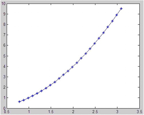
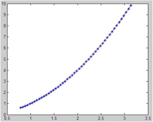
Figure 2 is a comparison of the accurate solution $q\left(x\right)$ and the corresponding approximate solution $q_{est}$ with the error 0.001.

Figure 2. Comparison of the accurate solution $q\left(x\right)$ and the corresponding approximate solution $q_{est}$ for h=0.005 and $N_0=10000$ with the nodal subset $\{x_{N_0,0}^j{\}}_{j=2500}^{10000}$.

Acknowledgements

The authors would like to thank the anonymous referees for valuable suggestions, which helped to improve the readability and quality of the paper.

Disclosure statement

No potential conflict of interest was reported by the authors.

References

- Hale J. Theory of functional-differential equations. New York (NY): Springer-Verlag; 1977.
- Buterin SA, Yurko VA. Sturm-Liouville differential operators with deviating argument. Tamkang J Math. 2017;46(1):61–71.
- Freiling G, Yurko VA. Inverse problems for Sturm-Liouville differential operators with a constant delay. Appl Math Lett. 2012;25:1999–2004. doi: 10.1016/j.aml.2012.03.026
- Pikula M. Determination of a Sturm-Liouville-type differential operator with delay argument from two spectra. Mat Vesnik. 1991;43(3–4):159–171.
- Vladičić V, Pikula M. An inverse problem for Sturm-Liouville-type differential equation with a constant delay. Sarajevo J Math. 2016;12(1):83–88. doi: 10.5644/SJM.12.1.06
- Vlasov VV. On the solvability and properties of solutions of functional-differential equations in a Hilbert space. Mat Sb. 1995;186(8):67–92. (in Russian); English transl in Sb Math. 186(8)(1995), 1147–1172
- Kuryshova YV, Shieh CT. An inverse nodal problem for integro-differential operators. J Inverse Ill-Posed Probl. 2010;18:357–369. doi: 10.1515/jiip.2010.014
- Freiling G, Yurko VA. Inverse Sturm-Liouville problems and their applications. New York (NY): Nova Science Publishers; 2001.
- Gesztesy F, Simon B. Inverse spectral analysis with partial information on the potential II: the case of discrete spectrum. Trans Amer Math Soc. 2000;352:2765–2787. doi: 10.1090/S0002-9947-99-02544-1
- Horvath M. On the inverse spectral theory of Schrödinger and Dirac operators. Trans Amer Math Soc. 2001;353:4155–4171. doi: 10.1090/S0002-9947-01-02765-9
- Rundell W, Sacks PE. The reconstruction of Sturm-Liouville operators. Inverse Probl. 1992;8:457–482. doi: 10.1088/0266-5611/8/3/007
- Wang YP. Inverse problems for discontinuous Sturm-Liouville operators with mixed spectral data. Inverse Probl Sci Eng. 2015;23:1180–1198. doi: 10.1080/17415977.2014.981748
- McLaughlin JR. Inverse spectral theory using nodal points as data-a uniqueness result. J Differential Equ. 1988;73:354–362. doi: 10.1016/0022-0396(88)90111-8
- Browne PJ, Sleeman BD. Inverse nodal problem for Sturm-Liouville equation with eigenparameter dependent boundary conditions. Inverse Probl. 1996;12:377–381. doi: 10.1088/0266-5611/12/4/002
- Cheng YH, Law CK, Tsay J. Remarks on a new inverse nodal problem. J Math Anal Appl. 2000;248:145–155. doi: 10.1006/jmaa.2000.6878
- Currie S, Watson BA. Inverse nodal problems for Sturm-Liouville equations on graphs. Inverse Probl. 2007;23:2029–2040. doi: 10.1088/0266-5611/23/5/013
- Guo Y, Wei G. Inverse problems: Dense nodal subset on an interior subinterval. J Differential Equ. 2013;255:2002–2017. doi: 10.1016/j.jde.2013.06.006
- Koyunbakan H, Panakhov ES. A uniqueness theorem for inverse nodal problem. Inverse Probl Sci Eng. 2007;15(6):517–524. doi: 10.1080/00423110500523143
- Law CK, Yang CF. Reconstructing the potential function and its derivatives using nodal data. Inverse Probl. 1998;14:299–312. doi: 10.1088/0266-5611/14/2/006
- Shen CL. On the nodal sets of the eigenfunctions of the string equations. SIAM J Math Anal. 1988;19:1419–1424. doi: 10.1137/0519104
- Shen CL, Shieh CT. An inverse nodal problem for vectorial Sturm-Liouville equation. Inverse Probl. 2000;16:349–356. doi: 10.1088/0266-5611/16/2/306
- Shieh CT, Yurko VA. Inverse nodal and inverse spectral problems for discontinuous boundary value problems. J Math Anal Appl. 2008;347:266–272. doi: 10.1016/j.jmaa.2008.05.097
- Wang WC, Cheng YH. On the existence of sign-changingradial solutions to nonlinear p-Laplacian equations in Rn. Nonlinear Anal Series A. 2014;102:14–22. doi: 10.1016/j.na.2014.01.027
- Wang YP, Lien Ko Ya, Shieh CT. Inverse problems for the boundary value problem with the interior nodal subsets. Appl Anal. 2017;96(7):1229–1239. doi: 10.1080/00036811.2016.1183770
- Wang YP, Shieh CT, Miao HY. Inverse transmission eigenvalue problems with the twin-dense nodal subset. J Inverse Ill-Posed Probl. 2017;25(2):237–249. doi: 10.1515/jiip-2016-0021
- Wang YP, Yurko VA. On the inverse nodal problems for discontinuous Sturm-Liouville operators. J Differential Equ. 2016;260:4086–4109. doi: 10.1016/j.jde.2015.11.004
- Yang CF. Solution to open problems of Yang concerning inverse nodal problems. Isr J Math. 2014;204:283–298. doi: 10.1007/s11856-014-1093-0
- Yang XF. A new inverse nodal problem. J Differential Equ. 2001;169:633–653. doi: 10.1006/jdeq.2000.3911
- Yurko VA. Inverse nodal problems for Sturm-Liouville operators on star-type graphs. J Inverse Ill-Posed Probl. 2008;16:715–722. doi: 10.1515/JIIP.2008.044