Particle filter-based monitoring scheme for simulated bio-ethylene production process

ABSTRACT

The use of biomass has been promoted to meet the need for sustainable production of ethylene, which is the most used petroleum-derived in the polymer industry. Ethanol is an alternative feedstock to yield the so-called bio-ethylene through catalytic dehydration in fixed-bed reactors. As the reaction system is strongly endothermic, it is very important to know accurately the reactor temperature to assure the process performance. However, in the industrial context, the process measurements are often uncertain and not all variables can be directly measured online. In this regard, this paper analyses the mathematical modelling and numerical simulation of the ethanol catalytic dehydration and contributes with a monitoring scheme using the Bayesian method known as particle filter. Numerical simulations helped understanding the process behaviour and locating the best position for the temperature sensor in the reactor. From temperature measurements, the proposed inferential tool estimates hidden state variables and unmeasured disturbances, using Sequential Importance Resampling algorithm for the particle filter. The proposal is investigated according to the number of particles and the criterion total error reduction. The results show that the monitoring scheme is able to estimate satisfactorily the process variable profiles, as the temperature and chemical conversion, along the reactor length.

KEYWORDS:

• Bio-ethylene
• modelling
• numerical simulation
• particle filter
• state estimation

MSC SUBJECT CLASSIFICATIONS:

• 62L12
• 65M12

Introduction

Ethylene is one of the main and most important starting materials of petrochemical industry. With a worldwide production of more than 143 million tons per year [1], it is used as intermediate to produce about 75% of petrochemicals, such as polyethylene, ethylene oxide, acetaldehyde, ethylene glycol, etc [2].

This olefin has been mainly produced by thermal cracking of hydrocarbons [3]. However, in the last years, to reduce greenhouse gas emission (or carbon footprint) and the dependence on fossil fuels [1], the use of biomass as a feedstock has become an attractive alternative for the production of the so-called bio-ethylene [4]. It is important to remark that ethylene and bio-ethylene present the same chemical features, as well as and the respective polymers, differing only in the environmental impact. This similarity allows for recycling and processing along with conventional polymers in the already existing industrial facilities [5].

Currently, to the best knowledge of the authors, Brazil and India are the countries that already deployed industrially this sustainable technology, representing approximately 0.3% of the global ethylene production. However, the global market for biopolymer production is growing fast and several production plants are under construction or planed [6]. Specifically, in Brazil, Braskem produces bio-ethylene from ethanol to provide polyethylene, being the largest producer of biopolymers in the world, with an annual capacity of 200 thousand tons [7,8].

The main forms of the bio-ethylene production from ethanol include the following routes: oxidative dehydrogenation, selective oxidation and catalytic dehydration. However, in the oxidative dehydrogenation, there is a significant by-product formation due to the presence of oxygen; and in the selective oxidation, the process uses vanadium-based catalysts that present a rapid deactivation increasing the operational cost of the process [9]. Thus, the ethanol catalytic dehydration has attracted much attention.

This process strongly endothermic is carried out in fixed bed or fluidized bed reactors over acid catalysts [10]. Under the low-temperature condition, the production of diethyl ether is predominant and, at high temperatures, the formation of ethylene is favoured [2,11–14]. The formation of hydrocarbons (due to secondary reactions) and the catalyst deactivation by coke (due to ethylene polymerization at excessively high temperatures) can also affect ethylene selectivity [15–17].

Most of the published works concerns about catalyst design [12,14,17–19], mechanism and kinetic studies [10,20,21] for this reaction system. Once it is very dependent on the operational conditions, mathematical modelling and simulation studies are paramount to improve the process understanding and the prediction of results. However, there are few works related to this issue for the ethanol catalytic dehydration.

Specifically, Golay et al. [22] proposed a pseudo-homogeneous model for the ethanol dehydration comprising five parallel reactions in a non-isothermal bench-scale reactor. Later, Kagyrmanova et al. [10] studied a pilot-scale plant with five irreversible reactions and recommended a two-dimensional heterogeneous model, considering mass and thermal dispersion. Recently, Maia et al. [9] proposed a complex fluid-dynamic modelling for a fixed-bed reactor using a dynamic pseudo-homogeneous model to describe thermal and mass axial dispersion. In addition, they took into account reversibility for the kinetic model of Kagyrmanova et al. [10], what improved the agreement between theoretical results and experimental data.

In many industrial applications, besides predicting the operational results, continuous real-time monitoring is a very important task to determine the conditions of the physical system, by recording information, recognizing and indicating anomalies in its behaviour [23]. The reliability of the monitoring approaches heavily depends on the accuracy of the mechanistic models and of the measurements [24]. However, the industrial process measurements generally contain noise and gross errors. This has a detrimental effect on the process control, making necessary to obtain accurate estimates for the states and measurements [25].

Among the observation techniques, the state estimation can be considered as a filtering problem within the Bayesian structure to reduce the measurement random errors [26]. To linear and Gaussian systems, the Kalman filter (KF) [27] is an optimal solution to the estimation problem. However, to the great majority of the chemical processes (non-linear and non-Gaussian systems), the most promising tool to be used on line is the Particle Filter (PF) [28].

The PF is a numerical method for the sequential state estimation that applies the Sequential Monte Carlo (SMC) method to estimate the posterior distribution of the evolving state by a set of particles and their corresponding assigned weights [29]. Although the use of filters has become quite popular, the application of these in chemical processes is still very recent [30–32]. Up to date, regarding the ethanol catalytic dehydration process (or even any other process in fixed-bed reactors), no work considering PF algorithms was found in the literature.

Based on the previous paragraphs, unlike most of the papers that concerns about catalytic and kinetics issues, the present work focuses on: (1) modelling and numerical simulation of the ethanol catalytic dehydration reactor; (2) process monitoring, using single-point temperature measurements to estimate hidden state variables and unmeasured disturbances through the algorithm Sequential Importance Resampling (SIR) of the particle filter.

Firstly, the dynamic simulation of the reactor model was numerically studied, considering an index-1 system of differential-algebraic equations (DAE). The main results were compared to previous papers available in the literature to check the model consistency. Besides that, it was investigated the best allocation of the temperature sensor in the reactor for the estimation problem.

Secondly, the filter SIR was used to estimate the reactor temperature and the chemical conversion profiles. This filter considers sequentially only two uncertain temperature measurements, one from a specific point in the reactor and another from the external heating fluid, and the process model. The estimation performance is investigated according to the number of particles (N_part), the effective number of particles ($N_{eff}$) and the criterion Total Error Reduction (TER).

As shown in the following sections, the proposed approach allows for a suitable simulation and proper estimation of the whole profiles of temperature, composition, selectivity and conversion, as well as for monitoring of the unmeasured disturbance entering the reactor. To conclude the paper, it is discussed that the reactor operation is consistent with the literature and the estimation scheme could be used as a monitoring tool in the bio-ethylene production process; some remarks and future work are outlined as well.

Process description

A simplified diagram of the ethanol dehydration process is shown in Figure 1. This process is performed in vapour phase in tubular reactors filled with alumina or silica–alumina catalysts [5]. The crude ethylene is separated from heavier products in a distillation tower and purified in a separate section [15]. The focus of this paper is only on the simulation and monitoring of the reactor, where the ethanol is converted to the ethylene and by-products.

Figure 1. Diagram of ethanol dehydration process [15].

The studies realized by Kagyrmanova et al. [10] revealed that the main products of the ethanol dehydration on the surface of the alumina-based catalyst are the ethylene, ethoxyethane, ethanal, hydrogen and butenes, as shown in the Equations (1)–(5). (1) ${\mathrm{C}}_2{\mathrm{H}}_5\mathrm{OH}\leftrightarrow {\mathrm{C}}_2{\mathrm{H}}_4+{\mathrm{H}}_2\mathrm{O},$(1) (2) $2{\mathrm{C}}_2{\mathrm{H}}_{5}OH\leftrightarrow ({\mathrm{C}}_2{\mathrm{H}}_5{)}_2\mathrm{O}+{\mathrm{H}}_2\mathrm{O},$(2) (3) ${\mathrm{C}}_2{\mathrm{H}}_5\mathrm{OH}\leftrightarrow {\mathrm{C}}_2{\mathrm{H}}_4\mathrm{O}+{\mathrm{H}}_2,$(3) (4) $({\mathrm{C}}_2{\mathrm{H}}_5{)}_2\mathrm{O}\leftrightarrow 2{\mathrm{C}}_2{\mathrm{H}}_4+{\mathrm{H}}_2\mathrm{O},$(4) (5) $2{\mathrm{C}}_2{\mathrm{H}}_4\leftrightarrow {\mathrm{C}}_4{\mathrm{H}}_8.$(5)

In order to facilitate the notation, the following reference was used (Table 1).

Table 1. Reference notation of the chemical species.

Chemical species	Notation	Chemical species	Notation
${\text{C}}_2{\text{H}}_5\text{OH}$ – Ethanol	1	${\text{C}}_2{\text{H}}_4\text{O}$ – Ethanal	5
${\text{C}}_2{\text{H}}_4$ – Ethylene	2	${\text{H}}_2$ – Hidrogênio	6
${\text{H}}_2\text{O}$ – Water	3	${\text{C}}_4{\text{H}}_8$ – Butenos	7
$({\text{C}}_2{\text{H}}_5{)}_2\text{O}$ – Ethoxyethane	4	_	_

The kinetic model has been based on elementary relations with reversibility considered by Maia et al. [9] and the law of mass action [33]. In this way, the expressions of the reaction rates were obtained, as described in the Equations (6)–(10). (6) $R_1=k_{1,D}\left(C_1-\frac{1}{K_{C,1}}{C}_2{C}_3\right),$(6) (7) $R_2=k_{2,D}\left({C_1}^2-\frac{1}{K_{C,2}}{C}_3{C}_4\right),$(7) (8) $R_3=k_{3,D}\left(C_1-\frac{1}{K_{C,3}}{C}_5{C}_6\right),$(8) (9) $R_4=k_{4,D}\left(C_4-\frac{1}{K_{C,4}}{C_2}^2{C}_3\right),$(9) (10) $R_5=k_{5,D}\left({C_2}^2-\frac{1}{K_{C,5}}{C}_7\right).$(10)

In these equations, R_j (j = 1, 2, … , 5) is the reaction rate, k_j is the specific reaction velocity with the subscript D indicating direct reactions, C_i (i = 1, 2, … , 7) is the concentration of each species and K_cj is the chemical equilibrium constant in terms of the concentration which is defined as the ratio between the direct and inverse specific velocity of the reaction.

Process model

Reactor modelling

In this work, the ethanol dehydration reactor was described by means of a model structure purposed by Schwaab et al. [34] for a tubular reactor along with the kinetic reaction model shown in the previous section. Some hypotheses adopted by Maia et al. [9] were also taken into account. However, this present work considered the reactor is placed inside a heat exchanger that provides the energy required for the endothermic reactions to keep the reaction at a suitable temperature.

The final model structure consists of an algebraic-differential system with partial derivatives and non-linear equations resulting from mass and energy balances, as well as constitutive equations. The mathematical model is given by the Equations (11)–(13). It is worthy to highlight that the proposed energy balance for the heating fluid temperature is a dynamic lumped model. (11) $\frac{\mathrm{\partial }{C}_i}{\mathrm{\partial }t}+\frac{\mathrm{\partial }{F}_i}{\mathrm{\partial }z}=\frac{\mathrm{\partial }}{\mathrm{\partial }z}\left(D_M\frac{\mathrm{\partial }{C}_i}{\mathrm{\partial }z}\right)+\sum _{j=1}^5{\upsilon }_{i,j}{R}_j,$(11) (12) $\begin{array}{l}\left[(1-\epsilon ){\rho }_S{C}_{P,S}+\epsilon {\rho }_M{C}_{P,M}\right]\frac{\mathrm{\partial }T}{\mathrm{\partial }t}+{\rho }_{M}v{C}_{P,M}\frac{\mathrm{\partial }T}{\mathrm{\partial }z}=\\ \frac{\mathrm{\partial }}{\mathrm{\partial }z}\left(k_H\frac{\mathrm{\partial }T}{\mathrm{\partial }z}\right)+\frac{4U}{D_t}(T_c-T)+\sum _{j=1}^5\left(-\mathrm{\Delta }{H}_j\right)R_j,\end{array}$(12) (13) ${\rho }_c{V}_c{C}_{P,c}\frac{\mathrm{\partial }{T}_v}{\mathrm{\partial }t}=q_c{\rho }_c{C}_{P,c}(T_{vf}-T_v)+U_c{A}_c(T-T_v).$(13)

In such equations, $F_i$ is the volumetric flow which is given by the equation F_i=v^.C_i. The index i refers to the species (i = 1, 2, … , 7), the index j refers to the number of reactions (j = 1, 2, … , 5). The parameters ρ_M, ρ_s and ρ_c are the specific mass of the mixture, the solid and the heating fluid; v is the mean velocity of the reaction mixture; C_i is the molar concentration of species i; D_M the effective mass diffusion coefficient; υ_ij the stoichiometric coefficient; R_j is the chemical kinetic rate for the reaction j; ε is the porosity of the catalytic bed; C_P,M, C_P,S and C_P,C are, respectively, the specific heat capacity of the mixture, the solid and the heating fluid at constant pressure; T the system temperature; T_v the jacket temperature and T_vf the jacket feed temperature; k_H is the coefficient of thermal conductivity; U is the internal heat transfer coefficient and U_c is the external heat transfer coefficient; D_t is the total bed diameter; ΔH_j is the molar heat of formation of the chemical reaction j; D_pparticle diameter; A_c the thermal exchange area and q_cis the volumetric flow rate of the heating jacket.

To complete the model, a set of initial conditions must be defined, as well as the boundary conditions for the concentration and the temperature at the inlet and outlet of the reactor, which are given by the Equations (14)–(17). In such conditions, C_if is the feed concentration of the species i and T_f is the feed temperature. (14) $z=0;v{C}_{if}\left(t\right)=v{C}_i(0,t)-D_M{\frac{\mathrm{\partial }{C}_i(z,t)}{\mathrm{\partial }z}|}_{z=0},$(14) (15) $z=L;{\frac{\mathrm{\partial }\left(C_i\right(t\left)\right)}{\mathrm{\partial }z}|}_{z=L}=0,$(15) (16) $z=0;{\rho }_{M}v{C}_{p,M}{T}_f\left(t\right)={\rho }_{M}v{C}_{P,M}T(0,t)-k_H{\frac{\mathrm{\partial }T(z,t)}{\mathrm{\partial }z}|}_{z=0},$(16) (17) $z=L;{\frac{\mathrm{\partial }T(z,t)}{\mathrm{\partial }z}|}_{z=L}=0.$(17)

The values for the reaction kinetics parameters and for the reactor used for the simulation are based on the work of Maia et al. [9]. The calculation of the thermodynamic parameters was performed with the correlations for ideal systems and for chemical equilibrium. The value of the external heat transfer coefficient (U_c) was obtained empirically throughout the simulations.

Model simulation

The solution of the model equation system for the process simulation was performed through the well-known Method of Lines [35], which consists of two steps: discretization of partial derivatives terms and solution of the modified system of equations.

In the first step, this work considered the Orthogonal Collocation Method [36] to approximate globally terms related to mass and thermal dispersion and convection along the axial direction. To accomplish that, the whole model was expressed in terms of dimensionless variables considering nominal values of the reactor, such as the length $L$ for the spatial variable ($\xi =z/L$) and the residence time ${\tau }_R$ for the time ($\tau =t/{\tau }_R$). The same idea was applied to the internal states using a reference condition for the concentration ($y_i=C_i/C_{ref}$) and for the temperatures ($\theta =T/T_{ref}$ and ${\theta }_v=T_v/T_{ref}$).

Within the transformed axial domain $0\le \xi \le 1$, it was determined $N$ collocation points as the zeros of the shifted Legendre orthogonal polynomial besides the two points at the boundary. Then, the spatial derivatives approximated at the collocation points using a polynomial based on $\mathbf{x}(\tau ,\xi )=\sum _{j=1}^{N+2}{l}_j\left(\xi \right)\mathbf{x}(\tau ,{\xi }_j)$ [35], where $l_j\left(\xi \right)$ is the Lagrangian interpolation polynomial, $\mathbf{x}(\tau ,{\xi }_j)$ is the solution for the states at the point ${\xi }_j$ and N + 1 is the order of the approximation. So, the first and second derivatives, for i = 1, … , N + 2, are given be the Equations (18) and (19): (18) $\frac{\mathrm{\partial }\mathbf{x}(\tau ,{\xi }_i)}{\mathrm{\partial }\xi }=\sum _{j=1}^{N+2}\mathbf{x}(\tau ,{\xi }_j)\frac{d{l}_j\left({\xi }_i\right)}{d\xi },$(18) (19) $\frac{{\mathrm{\partial }}^2\mathbf{x}(\tau ,{\xi }_i)}{\mathrm{\partial }{\xi }^2}=\sum _{j=1}^{N+2}\mathbf{x}(\tau ,{\xi }_j)\frac{d^2{l}_j\left({\xi }_i\right)}{d{\xi }^2}.$(19)

In the second step, the resulting index-1 DAE were solved numerically in terms of the time with MATLAB, applying the concept of the singular mass matrix [37]. Besides that, as the considered kinetics comprises coupled reactions, the DAE system is supposed to be stiff such way that the selected integration routine was the ode15s [38]. The data used for the simulation of the process were based on the work of Maia et al. [9], as the structural parameters of the reactor and parameters related to the operation (initial condition), reaction kinetics and fluid dynamics.

The convergence tests and model consistency tests were carried out, varying number of grid points (i.e. collocation points) and some inputs to understand the process dynamics. The simulation results were validated considering important operational parameters, as conversion and selectivity. Afterwards, the model was used to select the allocation of the temperature sensor in order to perform the process monitoring investigation.

Process monitoring

In industrial applications, the successful implementation of the advanced monitoring and control techniques highly depends on the representativeness of process models, as well as accuracy and reliability of measurements [39]. However, the measurements of process quality variables are often restricted by the inadequacy of the measurement techniques or low reliability of the measuring devices [40]. In such cases, the use of appropriate mathematical modelling along with measurement data can allow to infer information for the state variables and reduce measurement uncertainties.

This type of indirect measurement can be treated as a state estimation problem (also known as a virtual sensor) [32,41–43], which minimizes the effects of the uncertainty and lack of instruments. In such kind of problems, a processing algorithm uses all the available measured data together with prior knowledge about the physical phenomena, in order to obtain the posterior probability density function (PDF) to provide sequential estimates of the desired dynamic variables [44].

The so-called Bayesian filters are important tools to approach such problems. The Kalman filter and its variations, as the Extented Kalman Filter (EKF) and the Unscented Kalman Filter (UKF), are by far the most widely known methods [27,40,45–47]. For example, López-Zapata et al. [43] studied recently an EKF based virtual sensor to infer the concentration of the species involved in the reactions of a biodiesel process considering measurements of temperature and pH. However, EKF presents inherent limitations when applied to systems with severe nonlinearity and non-Gaussian noises [48]. To more realistic problems, Particle Filters represent the posterior PDF in terms of weighted random samples [49–53]. These methods can be applied to non-linear and non-Gaussian systems, as most of the practical chemical applications, including reactor and unit operations, polymerization systems and fermentation processes [30–32].

State estimation problem

Within the Bayesian framework, the dynamic problem is regarded as a Markovian process, using an evolution and an observation model as given respectively by the Equations (20) and (21) [42,49,52]: (20) ${\mathbf{x}}_k=\mathbf{f}({\mathbf{x}}_{k-1},{\mathbf{v}}_k),$(20) (21) ${\mathbf{z}}_k=\mathbf{h}({\mathbf{x}}_k,{\mathbf{n}}_k).$(21)

In this representation, $\text{f}$ is the non-linear model of the dynamical problem accounting for the state vector ${\mathbf{x}}_k\in {\mathbf{R}}^n$ and the uncertainty ${\text{v}}_k\in {\mathbf{R}}^n$. The state vector contains the variables to be dynamically estimated at each sampling time instant $k$. The function $\text{h}$ is possibly non-linear model describing the dependence between the measurements ${\mathbf{z}}_k\in {\mathbf{R}}^{nz}$and the updated state variables and the uncertainty ${\mathbf{n}}_k\in {\mathbf{R}}^{nz}$.

The estimation problem through particle filter is as follows. For the measured data ${\mathbf{z}}_k^{obs}$ at the time instant $k$, N_part particles for the states, $\{{\mathbf{x}}_{k-1}^{\left(i\right)}{\}}_{i=1}^{N_{part}}$, are drawn from a prior PDF. Such particles are propagated using the state evolution model and updated with the observation model in order to give the measurement estimates, $\{{\mathbf{z}}_k^{\left(i\right)}{\}}_{i=1}^{N_{part}}$. Afterwards, a likelihood function assigns an importance weight, $w_k^{\left(i\right)}\propto \pi \left({\mathbf{z}}_k^{\left(i\right)}|{\mathbf{z}}_k^{obs}\right)$. The set of the updated states and the weights, $\{{\mathbf{x}}_k^{\left(i\right)},w_k^{\left(i\right)}{\}}_{i=1}^{N_{part}}$, represents the approximation for the posterior PDF.

A problem that may take place is the degeneracy phenomenon [49]. One way of evaluating this drawback is to calculate the effective sample size ($N_{eff}$) (Equation (22)), which is the number of particles with nonzero weight [49,52]. To avoid degeneracy, it is paramount to resample particles, which is performed by the SIR algorithm. For further details about the particle filters, the reader is referred to other literature works as Chen et al. [26], Arulampalam et al. [49] and Chatzi and Smyth [47]. (22) $N_{eff}={\left[\sum _{i=1}^{N_{part}}{\left(w_k^i\right)}^2\right]}^{-1}.$(22)

Within this framework, we considered estimating parameter and state variables along the reactor and filtering the temperature measurements. In this inverse problem, the evolution model for the state variables is the numerical approximation of the process model through the orthogonal collocation method (Equation (23)), where ${\xi }_i$ represents the collocation points for i = 1, … ,N + 2. Finally, the Equation (24) is the observation model since the measurement estimates are observation of the respective estimated states, where $\mathbf{H}\in {\text{R}}^{nz\times n}$. (23) ${\mathbf{x}}_k\left({\xi }_i\right)=\mathbf{f}\left[{\mathbf{x}}_{k-1}\left({\xi }_i\right),\frac{\mathrm{\partial }{\mathbf{x}}_{k-1}\left({\xi }_i\right)}{\mathrm{\partial }\xi },\frac{{\mathrm{\partial }}^2{\mathbf{x}}_{k-1}\left({\xi }_i\right)}{\mathrm{\partial }{\xi }^2}\right]+{\mathbf{v}}_k,$(23) (24) $\mathbf{z}{}_k=\mathbf{H}\mathbf{x}{}_k+{\mathbf{n}}_k.$(24)

Proposed monitoring scheme

The ethanol conversion and the ethylene selectivity can be significantly affected by the process temperature and the feed concentration of the reactants. In this way, the estimation of the state variables and of the ethanol feed concentration is essential for the process monitoring. Thus, the proposed monitoring scheme estimates hidden state variables and an unmeasured disturbance through SIR filter from temperature measurements.

The filter is applied to estimate the profile along the reactor for the following state variables: the concentration (given as molar fractions) of the seven chemical species (y_i, i = 1,..,7) and the reactor temperature (T), as well as the heating fluid temperature (T_v), which comprise the state vector ${\mathbf{x}}^{\mathrm{T}}=\left[{\mathbf{y}}^{\mathrm{T}},T,T_v\right]$. In addition, we also considered estimating the ethanol feed molar fraction (y_f1), which is actually an operational parameter representing an unmeasured disturbance rather than a state. Hence, the estimation was performed with the augmented state vector ${\mathbf{x}}_{aug}^{\mathrm{T}}=\left[{\mathbf{x}}^{\mathrm{T}},y_{f1}\right]$. This monitoring scheme considers only two temperature measurements, being one from a specific point in the reactor and another from the heating fluid in the jacket.

In order to avoid the inverse crime [41], the reactor and heating fluid temperature data over time, used as observed measure (${\mathit{z}}_k^{obs}$), were obtained from the direct problem based on the model simulation considering a more refined grid (that is, a grid with the minimal number of collocation points necessary for the grid convergence). Conversely, the proposed scheme assumes that the simulation for each sample particle, aiming at the state estimation (inverse problem), is to be performed with fewer collocation points than the direct problem. The different grid refinement poses an important challenge for the estimation scheme, since it represents model mismatch between the direct and inverse problems. Besides that, this allows reducing the computational time required by the inverse problem, once it is performed accordingly to the number of particles.

In this work, the observed measures are pseudo-measurements taken at a specific position z_SP in the reactor, which should be chosen to locate the sensor based on the temperature sensitivity. These measurements were calculated considering only additive noise errors, which were supposed to be uncorrelated, additive, Gaussian, with zero mean and constant standard deviation of 5% of the maximum temperature, according to the expression ${\mathbf{z}}_k^{obs}={\hat{\mathbf{z}}}_k+{\mathit{\epsilon }}_k$. In this representation, ${\hat{\mathbf{z}}}_k$ is the solution of the direct problem (true value) for the reactor and the heating fluid temperatures, such that ${\hat{\mathbf{z}}}_k^T=[T_k,T_{v,k}]$; and ${\mathit{\epsilon }}_k$ is the noise error normally distributed.

In the inverse problem, the particles were drawn considering a priori knowledge of the process (as the initial guesses or the last estimatives of the state variables) to which is to be added accordingly a Gaussian uncertainty with standard deviation of 5% of the initial values. The evolution model for the spatial state variables was also solved by means of the method of lines and of the orthogonal collocation, but the grid was set arbitrarily with only five collocation points. It is important to highlight that the evolution model for the ethanol feed molar fraction is given by the random walk $y_{f1,k}=y_{f1,k-1}+{\sigma }_1{\epsilon }_1$. In this model, σ₁ is the standard deviation for the parameter and ε₁ is a random number with uniform distribution between [−1, 1].

The proposed monitoring scheme with SIR filter algorithm, which is to be applied to the system evolution iteratively from k to k + 1, is summarized in Figure 2.

Figure 2. Representation of the proposed monitoring scheme using SIR filter algorithm for the ethanol catalytic dehydration in fixed-bed reactor.

It is important to remark that the solution of the inverse problem for the reactor temperature has to be interpolated (Interpolation 1) to match the position z_SP in the reactor where the pseudo-measurements are taken. Afterwards, following the resampling step, the solution of the best selected particles is again interpolated (Interpolation 2) in order to identify the filtered measurement at the position z_SP.

We tested our proposal empirically with different particle numbers (N_part = 10, 50 and 100). The best performance setting was used to solve the estimation problem. It was considered a 99% credibility interval, calculated for each sampling time around the estimated states ($x_{est}$) according to the Equations (25) and (26). (25) $L_{inf}=x_{est}-t_{inv}(p,N_{part}-1)\cdot {\sigma }_{est},$(25) (26) $L_{sup}=x_{est}+t_{inv}(p,N_{part}-1)\cdot {\sigma }_{est}.$(26)

In these representations, L_inf and L_sup are, respectively, the limits of the credibility interval representing the uncertainty of the particles. The function t_inv is the inverse of Student’s T cumulative distribution function with N_part−1 degrees of freedom for the corresponding probability in p.

The filter performance was evaluated using the effective sample size ($N_{eff}$) and, as the true values of the pseudo-measurements are known, the criterion TER in Equation (27). This index measures the reduction of errors based on the measured values ($z_i^{obs}$) and the respective estimates ($z_i^{est}$) in relation to the true values (${\hat{z}}_i$) for the i-th measured variable. The closer TER is to 1, the better the result [54]. (24) $TER=\left(\sqrt{\sum _{i=1}^n\frac{{(z_i^{obs}-{\hat{z}}_i)}^2}{{\sigma }_i^2}}-\sqrt{\sum _{i=1}^n\frac{{(z_i^{est}-{\hat{z}}_i)}^2}{{\sigma }_i^2}}\right)/\phantom{\frac{1}{2}}\sqrt{\sum _{i=1}^n\frac{{(z_i^{obs}-{\hat{z}}_i)}^2}{{\sigma }_i^2}}.$(24)

Results and discussions

The ethanol catalytic dehydration considered here work results in a system composed of nine state variables: seven variables related to the composition of each chemical species, one variable related to the reactor temperature and one more representing the heating fluid temperature. The equation system for the concentration and temperature of the reactor is a model of distributed parameters; meanwhile, the model for the jacket temperature considers no spatial variations. Thus, for a number of internal grid points equal to N, we have a total of points equal to NP = N + 2 (internal grid points plus two boundary conditions) and the total variables considered in the system is 8NP + 1.

For the dynamic study, the simulation of the direct problem was used to obtain the results at the exit of the reactor, for a period of time fifteen times greater than the residence time. The variables were also evaluated throughout the reactor to investigate their spatial behaviours. The computational studies for direct and inverse problem were performed in MATLAB software on a computer with Intel Core i3-3110M 2.40 GHz processor, 4 GB RAM and W10 64-bit OS. The subsections below present the main results of this work.

Modelling and simulation

Grid convergence

To verify the grid convergence due to the spatial discretization and to choose the best proposal with the lowest computational cost, the simulation was done for different numbers of internal collocation points from 6 up to 20 points, which corresponded to the highest degree of refinement. The comparison of the simulations was made by means of the ratio between the difference of the maximum (T_max) and minimum (T_min) reactor temperature of the 20-point grid and the same difference of each mesh. The ratio values between the temperature differences, represented by ratio (20/N), the residue and the simulation time (t_s) are presented in Table 2, accordingly to the number of internal points.

Table 2. Analysis of the grid convergence considering residual values, temperature ratio and simulation time.

N	Residue	Ratio (20/N)	ts (s)
6	2.8294e−013	1.1382	2.9017
11	5.8121e−012	1.0208	4.8788
16	1.6214e−011	1.0359	6.4718
20	2.4434e−011	1.0000	8.5297

From Table 2, it is possible to observe that the model and the numerical approach are consistent since the residuals are practically zero for the different numbers of simulated points. It can also be seen that with 11 internal points the value of the ratio (20/N) is close to 1, which guarantees that the grid convergence has already been achieved. The computational cost was also considered in the choice of the number of collocation points. The computational cost for 11 points is smaller when compared to the 16 and 20 point grids. In this way, the grid with 11 internal collocation points meets the criteria for grid convergence and it was chosen to set the simulations of the direct problem. Therefore, with 11 internal collocation points (N = 11), the dimension of the direct problem was 105 dynamical variables.

Model consistency analysis

In this subsection, the stationary profiles of molar fraction and temperature along the reactor length were analysed. In addition, the important operational results of the proposed model were compared with the results obtained by Maia et al. [9] and Kagyrmanova et al. [10], since these works were the basis of the data and the kinetic model used in the present study.

Figure 3(a) and (b) show the evolution of the reactants and products at each point of the reactor. It is noted that the reaction occurs almost entirely in the first 20% of the reactor length.

Figure 3. Stationary profiles of the molar fractions along the reactor for: (a) ethanol, ethylene, water, ethoxyethane and (b) ethanal, hydrogen, butenes.

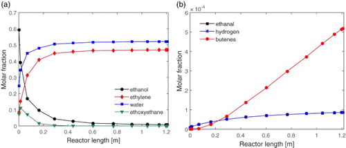
Figure 3 (a) shows a higher formation of the ethoxyethane at the beginning of the reactor, but throughout the reactor this amount is reduced to almost zero at the exit of the process. This is mainly due to the decomposition of this by-product into the ethylene by the chemical reaction 4. As this reaction is endothermic, it is favoured by the high process temperature in relation to the chemical reaction 2, which in turn is exothermic. In addition, it can also be seen that the ethanol is not fully consumed, with about 1% of the main reactant remaining in the outlet stream, even in a favourable temperature range. This suggests that the ethanol reached its equilibrium concentration. Little by-product formation can be observed in Figure 3 (b), which shows the ethanal, butenes and hydrogen with fractions smaller than 0.01 in the final composition of the product.

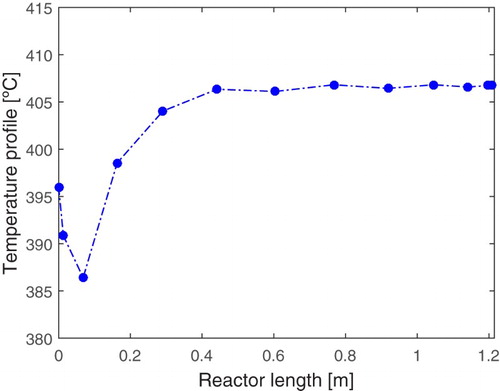
The reactor temperature steady profile is shown in Figure 4. It can be observed that, in the region where almost all the reactions occur, there is a rapid reduction of reactor temperature. This characterizes the strongly endothermic character of the ethylene formation process. As the ethanol concentration decreases, the reaction rate is reduced and the reactor temperature increases due to the thermal exchange effect with the jacket. The result of this process was a product stream consisting of approximately 52% water, 47% ethylene and 1% by-products, in molar percentage. The behaviour of the system and the results obtained are in agreement with those found in the work of Maia et al. [9], which shows the consistency of the implemented system.

Figure 4. Stationary profile of reactor temperature.

The results for the ethanol conversion and the ethylene selectivity are presented in Table 3, where they are compared to the referenced literature. It is shown that the results of the present work are equivalent to the models published by Kagyrmanova et al. [10] and Maia et al. [9]. It is important to highlight that the hypothesis of varying jacket temperature kept the reactor warmer spatially, which justified the best results for the ethoxyethane and butenes selectivity. These results allow stating that the proposed model is validated.

Table 3. Conversion and selectivity comparison with data from literature.

Compared parameters	Kagyrmanova et al. (2011)	Maia et al. (2016)	This work
Ethanol conversion (%)	98.5	98.7	98.34
Ethylene selectivity (%)	98.8	98.5	99.7
Ethoxyethane selectivity (%)	0.26	0.21	0.018
Butenes selectivity (%)	0.21	0.18	0.10

In addition, in Maia et al. [9], the model discretization for this process was done by the finite difference method using 100 discretization points. In our work, the use of the orthogonal collocation with 11 internal points showed the efficiency of this method for the DAE system solution. It took a shorter simulation time (4.8 s) in relation to the 8 s spent in the work of Maia et al. Consequently, this work presents a solution that requires lower computational cost and satisfies globally the mathematical structure of the problem (since it was treated as an index-1 DAE system instead of reducing to a fully ODE system).

Parameter effect analysis

In order to verify the effect of the model parameters and the proposed considerations for the ethanol catalytic dehydration process, Figures 5–7 present the result for the reactor flow velocity (v_f), the jacket feed temperature (T_vf) and the feed stream composition (y_f1), which were evaluated in relation to the spatial profile of the reactor temperature, the ethylene selectivity and the ethanol conversion.

Figure 5. Effect of feed rate (vf = 0.1, 0.3, 0.6, 0.8, 1.0): (a) in the reactor spatial temperature profile and (b) in the ethylene selectivity and ethanol conversion.

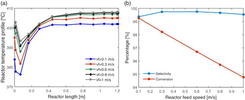
Figure 6. Effect of jacket feed temperature (Tvf = 380°C, 390°C, 400°C, 410°C, 420°C): (a) in the reactor spatial temperature profile and (b) in the ethylene selectivity and ethanol conversion.

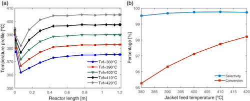
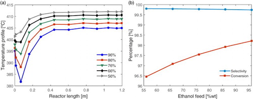
Figure 7. Effect of ethanol feed concentration (56, 66, 76, 86, 96% wt.): (a) in the reactor spatial temperature profile and (b) in the ethylene selectivity and ethanol conversion.

In Figure 5(a), it is possible to observe that as the feed rate of the reactional mixture is increased, the reactor becomes warmer and with lower internal temperature variation. However, Figure 5(b) shows that, even if the selectivity for the ethylene remains high, the conversion of ethanol decreases as the feed rate increases. This happens because the higher the feed rate, the shorter the contact time of the reactant with the catalytic bed, and consequently the lower the residence time and the ethanol conversion. Thus, although the bed temperature is reduced near the reactor entrance, it is preferred to maintain the feed rate at about 0.3 m/s, in order to obtain better selectivity for the ethylene and ethanol conversion.

In alumina-catalyzed processes, at feed temperatures above 420°C, the selectivity for the ethylene begins to decrease due to the increase in the formation of butenes and other by-products [10]. In this way, we performed tests for the jacket feed temperature up to 420°C. Figure 6(a) shows that for higher temperatures at the inlet of the heating jacket, the higher the reactor temperature over its entire length. This condition ensures enhancing the thermal exchange, which favours the extent of the reaction at the entrance of the reactor. So, the effects of higher feed temperature of the jacket are both: the reduction of the cold points and the maintenance of the reactor temperature at favourable level for ethanol conversion. According to Figure 6(b), although the ethylene selectivity does not change much, the ethanol conversion increases leading to higher ethylene formation.

The effect of the feeding stream composition to the reactor can be analysed in Figure 7. It is observed that, for a larger amount of ethanol in the reactor feed: the higher the ethanol conversion and the lower the temperature and the cold point. This is as expected, because higher the ethanol concentration, the conversion to ethylene increases, which consequently increases the heat consumption by the endothermic reaction. These results are in agreement with those ones obtained by Kagyrmanorva et al. [10] who stated that higher ethanol conversion and ethylene selectivity are obtained for ethanol feed concentrations above 94%. This result shows that the bio-ethanol resulting from the distillation, which is in the hydrated form with 6% of water in weight due to the formation of an azeotropic mixture, already presents the ideal composition for the production process of the ethylene.

Temperature sensor placement

The monitoring of the reactor temperature be done by measuring this variable with the installation of a temperature sensor at a strategic point in the reactor. In order to obtain the best position for the installation, an analysis of the temperature profile was carried out over time at some reactor points as shown in Figure 8.

Figure 8. Temperature profile over time in some points of the reactor for sensor placement (Pt: spatial position in the reactor).

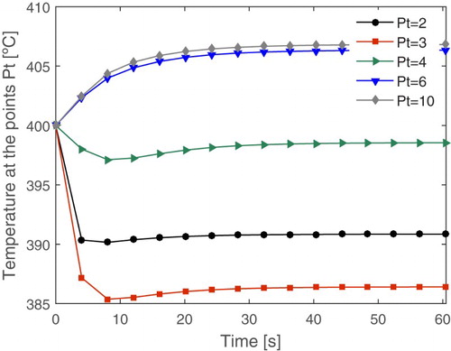
Considering an 11-point grid, it is worthy to highlight that the first and last points are related to the boundary conditions. This way, by the analysis of Figure 8, the position 3 of the reactor features a cold spot, where the temperature drops rapidly and remains low over time, due to the strongly endothermic characteristic of the process. Since low temperatures favour the formation of the ethoxyethylene, this position is considered a critical point and must be monitored. Thus, in order to obtain better monitoring of the temperature of the fixed-bed reactor, this work suggests the installation of the temperature sensor in the spatial position 3 of the reactor, which is equivalent to the length of about 0.1 m of the reactor.

Estimation problem

Three different numbers of particles were evaluated and the best performance filter was selected based on the effective size sample ($N_{eff}$) and the TER. In order to obtain a fair comparison among the results, the noise error sequence used for the pseudo-measurements was maintained the same. The results of the filter performances are shown in Table 4.

Table 4. Filter performance according to number of particles.

Npart	TER	Neff/Npart (%)	Filter time (s)
10	0.8757	92.18	2.68
50	0.9141	91.17	11.96
100	0.9147	91.20	24.70

With the increase in the number of particles from 10 to 50, an increase in the value of the TER was observed, showing an improvement in filter performance. For 50 and 100 particles, there was no significant difference in the value of TER. In addition, in all cases, the effective sample size was over 90% of the number of particles, meaning that the degeneracy phenomenon was not important. Thus, for the estimation problem, the filter with 50 particles was selected, which presented suitable values to the criterion TER and to the computational time.

Figure 9 shows the dynamic behaviour of the estimated variables: (a) the reactor temperature, (b) the temperature of the heating fluid and (c) the molar fraction of ethanol feed. In the sequence, Figure 10 shows the spatial profile of the estimated variables (a) the reactor temperature and (b) the ethanol molar fraction. In these figures, the diamonds represent the measured values (with uncertainty), the points the estimated values (identified in the second interpolation), the solid line indicates the exact value given by the direct problem and the thicker continuous black line, the interpolated estimated values. The demarcated region between the two black fine lines indicates the 99% credibility interval. It can be seen that, in the dynamic profiles, the estimated values presented an excellent agreement with the exact values, not only for the measured variables (the reactor temperature and the jacket temperature), but also for the unmeasured variables (as the molar fraction of ethanol feed). For the spatial profiles, it can be observed that from measurements with noises in a single point of the system, located close to the entrance of the reactor, the SIR filter was able to estimate the spatial profile of temperature and composition of ethanol throughout the whole length of the reactor. It is worth noting again that the molar fraction of ethanol is an unmeasured variable.

Figure 9. Dynamic profile of estimated value for: (a) reactor temperature, (b) jacket temperature and (c) molar fraction of ethanol feed.

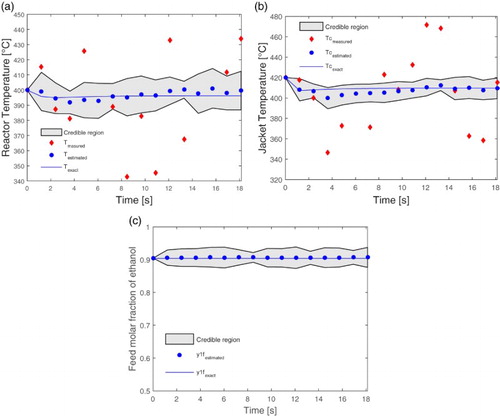
Figure 10. Spatial profile of estimated value for: (a) reactor temperature and (b) ethanol molar fraction.

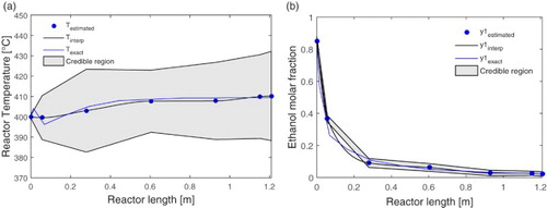
Figure 10(a) shows a smaller credibility interval near the measurement point, which is similar to the credibility interval of Figure 9(a), which shows the state variable for this point over time. It is also noted that the credibility interval increases throughout the reactor, this is related to the increase in measurement, model and interpolations uncertainties. A higher number of particles in the estimation process can reduce this credibility interval, but the increase of the computational cost not justifying the cost benefit of the state estimation tool.

Thus, the presented results show that the 5% level of uncertainty provides a fine range of credibility, since most of measurements with uncertainty are outside this range. Therefore, it can be stated that the SIR filter was able to reduce the effects of measurement noise and, more importantly, to estimate hidden states. The ethanol feeding molar fraction was not considered as a measured variable, but it was also possible to estimate dynamical values satisfactorily. For instance, this would be a potential tool to provide anticipative information to a feedforward controller before facing problems in the ethanol conversion. In addition, it is important to remark that, even in face of strong limitation due to the 5-point grid in the inverse problem, the estimation scheme showed robust performance.

Conclusions

In present work, a phenomenological model was proposed to describe the ethanol catalytic dehydration to produce bio-ethylene in fixed-bed reactor. The model comprises a set of DAE describing one-dimensional dispersion of mass and energy balances for the reactor bed and it is coupled to thermodynamic equations to account for reversibility of the chemical reactions. A simplified model to describe dynamic variations of the heating fluid temperature was also included. In addition, the monitoring problem of this process was investigated by means of the SIR particle filter, which is performed with only two uncertain single-point temperature measurements as process information.

The dynamic and steady behaviour of the ethanol catalytic dehydration reactor, including the reactor temperature profile, the ethanol conversion, the ethylene selectivity, was analysed in different conditions of flow velocity, heating fluid feeding temperature and ethanol feeding concentration. The methods of lines and of orthogonal collocation were used to solve the model equations. According to the obtained simulation results, the model is consistent with the literature, which implies that it is able to describe very well the process on study. The effect of these operational parameters confirmed high ethanol conversion and ethylene selectivity at ethanol feeding concentrations above 94% and at high reactor temperatures, specifically between 380°C and 420°C. In addition, the simulations also allowed the grid convergence analysis with 11 internal collocation points and the temperature sensor placement at the third point of the grid.

In the state estimation problem, in order to avoid inverse crime, the SIR filter was implemented with a 5-point grid for the state evolution model of the particles. Regarding the difference between the grid refinements of the direct and inverse problems, two interpolation steps were added to the filter algorithm to obtain the exact point of comparison between the pseudo-measurement and particles. The filter performance was investigated for different particle number in order to verify computational cost and TER. It was found that 50 particles suffice to estimate the reactor and jacket temperatures as well as the concentration profiles in the reactor and the ethanol feeding concentration, which is not a measured variable. Satisfactory results were obtained despite the limitation cause by the grid with low amount of points in the inverse problem. This way, the proposed estimation scheme was able to follow the actual process path.

Disclosure statement

No potential conflict of interest was reported by the authors.

ORCID

Luciana Souza Ferreira Salardani http://orcid.org/0000-0002-8794-4930

Lorrane Pains Albuquerque http://orcid.org/0000-0002-3047-9951

José Mir Justino da Costa http://orcid.org/0000-0001-5719-4377

Wellington Betencurte da Silva http://orcid.org/0000-0003-2242-7825

Julio Cesar Sampaio Dutra http://orcid.org/0000-0001-6784-4150

Additional information

Funding

The authors thank CAPES (Coordenação de Aperfeiçoamento de Pessoal de Nível Superior) for providing scholarship.

References

- IRENA. Technology brief: production of bioethylene. Abu Dhabi: IRENA; 2013.
- Zhang M, Yu Y. Dehydration of ethanol to ethylene. Ind Eng Chem. 2013;52:9505–9514. doi: 10.1021/ie401157c
- Chen G, Li S, Jiao F, et al. Catalytic dehydration of bioethanol to ethylene over TiO2/γ - Al2O3 catalysts in microchannel reactors. Catal Today. 2007;125:111–119. doi: 10.1016/j.cattod.2007.01.071
- Sun J, Wang Y. Recent advances in catalytic conversion of ethanol to chemicals. ACS Catal. 2014;4:1078–1090. doi: 10.1021/cs4011343
- Morschbacker A. Bio-Ethanol based ethylene. Polym Rev. 2009;49(2):79–84. doi: 10.1080/15583720902834791
- IRENA. Renewable energy in manufacturing. 2015.
- Braskem. Annual Report 2011. 2011.
- Braskem. Annual Report 2015. 2015.
- Maia JGSS, Demuner RB, Secchi AR, Jr, et al. Modeling and simulation of the process of dehydration of bioethanol to ethylene. Braz J Chem Eng. 2016;33:479–490. doi: 10.1590/0104-6632.20160333s20150139
- Kagyrmanova AP, Chumachenko VA, Korotkikh VN, et al. Catalytic dehydration of bioethanol to ethylene: pilot-scale studies and process simulation. Chem Eng J. 2011;1:188–194. doi: 10.1016/j.cej.2011.06.049
- Matachowski L, Zimowska M, Mucha D, et al. Ecofriendly production of ethylene by dehydration of ethanol over Ag3PW12O40. Appl Catal B. 2012;123– 124:448–456. doi: 10.1016/j.apcatb.2012.05.003
- Sheng Q, Ling K, Lib Z, et al. Effect of steam treatment on catalytic performance of HZSM-5 catalyst for ethanol dehydration to ethylene. Fuel Process. Technol. 2013;110:73–78. doi: 10.1016/j.fuproc.2012.11.004
- Phung TK, Hernández P L, Lagazzo A, et al. Dehydration of ethanol over zeolites, silica alumina and alumina:Lewis acidity, brønsted acidity and confinement effects. Appl Catal A. 2015;493:77–89. doi: 10.1016/j.apcata.2014.12.047
- Phung TK, Busca G. Ethanol dehydration on silica-aluminas: active sites and ethylene/diethyl ether selectivities. Catalysis Commun. 2015;68:110–115. doi: 10.1016/j.catcom.2015.05.009
- Jernberg J, Norregard O, Olofsson M, et al. Ethanol dehydration to green ethylene. COWI and Borealis – Final Report. 2015.
- Moulijn JA, Makkee M, Van Diepen A. Chemical process technology. 2nd ed. Chichester: John Wiley & Sons; 2013.
- Ramesh K, Goh YLE, Gwie CG, et al. Ethanol dehydration activity on hydrothermally stable LaPxOy catalysts synthesized using CTAB template. J Porous Mater. 2012;19:423–431. doi: 10.1007/s10934-011-9490-9
- Chen Y, Wu Y, Tao L, et al. Dehydration reaction of bio-ethanol to ethylene over modified SAPO catalysts. J Ind Eng Chem; 2010;16:717–722. doi: 10.1016/j.jiec.2010.07.013
- Chinniyomphanich U, Wongwanichsin P, Jitkarnka S. Snxoy/SAPO-34 as catalysts for catalytic dehydration of bio-ethanol: impacts of oxidation state, interaction, and loading amount. J Clean Prod. 2016;111:23–33. doi: 10.1016/j.jclepro.2015.09.069
- Ouyang J, Kong F, Su G, et al. Catalytic conversion of bio-ethanol to ethylene over La-modified HZSM-5 catalysts in bioreactor. Catal Letter. 2009;132:64–74. doi: 10.1007/s10562-009-0047-3
- Dewilde JF, Chiang H, Hickman DA, et al. Kinetics and mechanism of ethanol dehydration on γ-Al2O3: the critical role of dimer inhibition. ACS Catal. 2013;3:798–807. doi: 10.1021/cs400051k
- Golay S, Doepper R, Renken A. Reactor performance enhancement under periodic operation for the ethanol dehydration over γ-alumina, a reaction with a stop-effect. Chem Eng Sci. 1999;54:4469–4474. doi: 10.1016/S0009-2509(99)00105-0
- Isermann R, Ballé P. Trends in the application of model-based fault detection and diagnosis of technical processes. Control Eng Pract. 1997;5:709–719. doi: 10.1016/S0967-0661(97)00053-1
- Mori J, Yu J. Quality relevant nonlinear batch process performance monitoring using a kernel based multiway non-Gaussian latent subspace projection approach. J Process Control. 2014;24:57–71. doi: 10.1016/j.jprocont.2013.10.017
- Zhao Z, Huang B, Liu F. Constrained particle filtering methods for state estimation of nonlinear process. AIChE J. 2014;60:2072–2082. doi: 10.1002/aic.14390
- Chen T, Morris J, Martin E. Particle filters for state and parameter estimation in batch processes. J Process Control. 2005;15:665–673. doi: 10.1016/j.jprocont.2005.01.001
- Kalman RE. A new approach to linear filtering and prediction problem. Trans ASME – J Basic Eng. 1960;82:34–45.
- Nishida T. State feedback control using particle filter. Electron e Commun. 2015;98:16–25. doi: 10.1002/ecj.11658
- Hanachi H, Liu J, Banerjee A, et al. Sequential state estimation of nonlinear/non-Gaussian systems with stochastic input for turbine degradation estimation. Mech Syst Signal Process. 2016;72–73:32-45. doi: 10.1016/j.ymssp.2015.10.022
- Shenoy AV, Prakashb J, Prasada V, et al. Practical issues in state estimation using particle filters: case studies with polymer reactors. J Process Control. 2013;23:120–131. doi: 10.1016/j.jprocont.2012.09.003
- Marques RAG, da Silva WB, Hoffmann RX, et al. Sequential state inference of engineering systems through the particle move-reweighting algorithm. Comput Appl Math. 2017;17:1–17.
- Dias ACSR, Da Silva WB, Dutra JCS. Propylene polymerization reactor control and estimation using a particle filter and neural network. Macromol React Eng. 2017;11:1–20. doi: 10.1002/mren.201700010
- Järvinen M, Visuri V, Heikkinen E, et al. Law of mass action based kinetic approach for the modelling of parallel mass transfer limited reactions: application to metallurgical systems. ISIJ Int. 2016;56:1543–1552. doi: 10.2355/isijinternational.ISIJINT-2016-241
- Schwaab M, Alberton AL, Fontes CE, et al. Hybrid modeling of methane reformers. 2. Modeling of the industrial reactors. Ind Eng Chem Res. 2009;48:9376–9382. doi: 10.1021/ie801831m
- Saucez P, Wouwer VA, Zegeling PA. Adaptive method of lines solutions for the extended fifth-order Korteweg–de Vries equation. J Comput Appl Math. 2005;183:343–357. doi: 10.1016/j.cam.2004.12.028
- Rice RG, Do DD. Applied mathematics and modeling for chemical engineers. Hoboken, NJ: John Wiley & Sons; 1995.
- Huang D, Wunsch DC, Levine DS, et al. Advanced intelligent computing theories and applications. New York: Springer Verlag; 2008.
- Shamiri A, Hussain MA, Mjalli FS, et al. Kinetic modeling of propylene homopolymerization in a gas-phase fluidized-bed reactor. Chem Eng J. 2010;161(1–2):240–249. doi: 10.1016/j.cej.2010.04.037
- Qin SJ, Badgwell TA. An overview of nonlinear model predictive control applications. In: F Allgöwer, A Zheng, CI Byrenes, editor. Nonlinear model predictive control. Progress in systems and control theory. Basel: Birkhäuser Basel; 2000. p. 369–392.
- Khatibisepehr S, Huang B, Khare S. Design of inferential sensors in the process industry: A review of Bayesian methods. J Process Control. 2013;23:1575–1596. doi: 10.1016/j.jprocont.2013.05.007
- Kaipio J, Somersalo E. Statistical and computational inverse problems, applied mathematical sciences. New York: Springer-Verlag; 2004.
- López-Zapata BY, Adam-Medina M, Álvarez-Gutiérrez PE, et al. Virtual sensors for biodiesel production in a batch reactor. Sustainability. 2017;9:455. doi: 10.3390/su9030455
- Maybeck P. Stochastic models, estimation and control. New York: Academic Press; 1979.
- Orlande HRB, Dulikravich GS, Neumayer M, et al. Accelerated Bayesian inference for the estimation of spatially varying heat flux in a heat conduction problem. Numer Heat Transf, Part A: Appl. 2014;65-1:1–25. doi: 10.1080/10407782.2013.812008
- Aslan S. Comparison of the hemodynamic filtering methods and particle filter with extended Kalman filter approximated proposal function as an efficient hemodynamic state estimation method. Biomed Signal Process Control. 2016;25:99–107. doi: 10.1016/j.bspc.2015.10.003
- Chatzi EN, Smyth AW. The unscented Kalman filter and particle filter methods for nonlinear structural system identification with non-collocated heterogeneous sensing. Struct Control Health Monit. 2009;16(1):99–123. doi: 10.1002/stc.290
- Shao X, Huang B, Lee JM. Constrained Bayesian state estimation – a comparative study and a new particle filter based approach. J Process Control. 2010;20:143–157. doi: 10.1016/j.jprocont.2009.11.002
- Arulampalam S, Maskell S, Gordon N, et al. A tutorial on particle filters for on-line non-linear/non-Gaussian Bayesian tracking. IEEE Trans Signal Process. 2002;50(2):174–188. doi: 10.1109/78.978374
- Doucet A, Freitas N, Gordon N. Sequential Monte Carlo methods in practice. New York: Springer; 2001.
- Ristic B, Arulampalam S, Gordon N. Beyond the Kalman filter. Boston: Artech House; 2004.
- Gordon N, Salmond D, Smith AFM. Novel approach to nonlinear and non-Gaussian Bayesian state estimation. Proc Inst Elect Eng. 1993;140:107–113.
- Özyurt DB, Pike RW. Theory and practice of simultaneous data reconciliation and gross error detection for chemical process. Comput Chem Eng. 2004;28:381–402. doi: 10.1016/j.compchemeng.2003.07.001