
 ?Mathematical formulae have been encoded as MathML and are displayed in this HTML version using MathJax in order to improve their display. Uncheck the box to turn MathJax off. This feature requires Javascript. Click on a formula to zoom.
ABSTRACT
This paper aims at estimating the sorption isotherm coefficients of a wood fiber material using experimental data. First, the mathematical model, based on convective transport of moisture, the Optimal Experiment Design (OED) and the experimental set-up are presented. Then, measurements of relative humidity within the material are carried out, after searching the OED using the computation of the sensitivity functions and a priori values of the unknown parameters. It enables to plan the experimental conditions in terms of sensor positioning and boundary conditions out of 20 possible designs, ensuring the best accuracy for the identification method and, thus, for the estimated parameter. After the measurements, the parameter estimation problem is solved. The determined sorption isotherm coefficients calibrate the numerical model to fit better the experimental data. However, some discrepancies still appear since the hysteresis effects on the sorption capacity are not included in the model. Therefore, the latter is improved proposing an additional differential equation for the sorption capacity to consider the hysteresis effects. The OED approach is developed for the estimation of five of the coefficients involved in the hysteresis model. To conclude, the prediction of the model with hysteresis have better reliability when compared to the experimental observations.
1. Introduction
Moisture in buildings has been a subject of major concern since 1980s. It may affect energy consumption and demand so we can mention at least four International Energy Agency projects conducted in the last 30 years to promote global research on this subject (Annexes 14, 24, 41 and 55) [Citation1]. Furthermore, moisture can also have a dramatic impact on occupants' health and on material deterioration. Several tools have been developed to simulate the moisture transport in constructions as described in [Citation2], which can be used to predict conduction loads associated to porous elements and mould growth risk in building enclosures. Nevertheless, those tools require input parameters containing temperature- and moisture-dependent hygrothermal properties.
1.1. Moisture transport in constructions
The following system of partial differential equations established by Luikov [Citation3] represents the physical phenomenon of heat and mass transfer through capillary porous materials: (1)
(1)
(2)
(2)
where U is the the specific mass content in the porous body, corresponding to the ratio of mass of water (in vapour and liquid phases) to the dry-basis mass of porous material. The other quantities are T the temperature,
the mass transfer coefficient for vapor (denoted with the subscript 1) and liquid inside the body, δ the thermal-gradient coefficient,
the specific mass of the dry body,
the specific heat of the body and
the latent heat of vapourization.
In building physics, those equations represent the physics that occurs in the porous building envelope and indoor porous elements such as furniture, textiles, etc. Regarding the envelope, the phenomenon is investigated to analyse the influence of moisture transfer on the total heat flux passing through the wall, with the objective of estimating heat losses. They are also studied to analyse the durability of walls and to avoid disorders due to the presence of moisture as, for instance, mould growth, shrinking or interstitial condensation. This aspect is of major importance for wall configurations involving several materials with different properties, where moisture can be accumulated at the interface between two materials. Durability problems may also appear when considering important moisture sources as wind-driven rain or rising damp problems. These analyses are performed by computing solutions to the partial differential equations similar to (Equation1(1)
(1) ). For this, numerical methods are used due to the nonlinearity of the material properties, depending on moisture content and temperature, and the non-stationary boundary conditions, defined as Robin-type and varying according to climatic data. Most of the numerical approaches consider standard discretization techniques. For the time discretisation, the Euler implicit [Citation4–6] or explicit [Citation7] schemes are adopted. Regarding the spatial discretisation, works in [Citation8] are based on finite-differences methods, in [Citation5,Citation6,Citation9,Citation10] on finite-volume methods and in [Citation11,Citation12] on finite-element methods. It is important to note that the numerical solution of these partial differential equations requires, after discretisation, the calculation of large systems of nonlinear algebraic equations (an order of
for 3-D problems). Furthermore, the problem deals with different time scales. The diffusive phenomena and the boundary conditions evolve on the time scale of minutes while the building performance usual analysis is done for a time interval of one year or even longer when dealing with durability or mould growth issues. Thus, the computation of heat and moisture transfer in porous material in building physics has a non-negligible computational cost. Recently, innovative and efficient methods of numerical simulation have been proposed. Some improved explicit schemes, enabling to overcome the stability restrictions of standard Euler explicit schemes, have been proposed in [Citation13,Citation14]. An accurate and fast numerical scheme based on the Scharfetter–Gummel idea has been proposed in [Citation15] to solve the
advective–diffusive moisture differential equation. Some attempts based on model reduction methods have been also proposed with an overview in [Citation8].
1.2. Inverse problems in building physics
While some research focuses on numerical methods to compute the solution of the so-called direct problem to analyse the physical phenomena, some studies aim at solving inverse problems of heat and mass transfer in porous materials. In this case, the focus is the estimation of material properties using experimental data denoted as
by minimizing a thoroughly chosen cost function
:
where
is certain vector-norm in time.
Here, the inverse problem is an inverse medium problem, as it aims at estimating the coefficients of the main equation [Citation16,Citation17]. Two contexts can be distinguished. First, when dealing with existing buildings to be retrofitted, samples cannot be extracted from the walls to determine their material properties. Therefore, some in situ measurements are carried out according to a non-destructive design. The experimental data can be gathered by temperature, relative humidity, flux sensors and infrared thermography, among others. In most cases, measurements are made at the boundary of the domain. From the obtained data, parameter estimation enables to determine the material thermophysical properties. As mentioned before, the properties are moisture and temperature-dependent. Therefore, the parameter identification problem needs to estimate functions that can be parameterized. Moreover, in such investigations, there is generally a few a priori information on the material properties. In [Citation18], the thermal conductivity of an old historic building wall composed of different materials is presented. In [Citation19], the thermophysical properties of materials composing a wall are estimated. In [Citation20], the heat capacity and the thermal conductivity of a heterogeneous wall are determined. Once the needed parameters have been estimated, efficient simulations using the direct model can be performed to predict the wall conduction loads and, at the end, choose adequate retrofitting options.
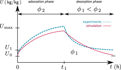
Another issue arises while comparing the numerical model results and experimental data. Some discrepancies were observed as reported in several studies [Citation15,Citation21] and illustrated in Figure . A material, with an initial moisture content , is submitted to adsorption and desorption cycles. The moisture content raises up to
at the end of the adsorption phase. Then, during the desorption phase, the moisture content decreases until a value
due to the hysteresis effects. When comparing the simulation results to the experimental data, it is observed that predictions of moisture content commonly underestimate the experimental observations of moisture adsorption processes. In other words, the numerical predictions are lower than the experimental values obtained during the adsorption phase. On the other hand, in the course of the desorption phase, the numerical predictions often overestimate the experimental observations, i.e. the simulation values are greater than the experimental ones. At the end of the desorption process, the experimental values are greater again, when compared to both the predicted values and the initial moisture content since the hysteresis phenomenon significantly affects the material moisture sorption capacity. It means the experimental moisture front rushes faster than the numerical predictions. To answer this issue, models can be calibrated using in situ measurements for adapting the material properties to reduce the discrepancies between model predictions and real observations. In [Citation22], moisture- and temperature-dependent diffusivity and thermophysical properties are estimated using only temperature measurements under a drying process. In [Citation23], the moisture permeability and advective coefficients are estimated using relative humidity measurements in a wood fibre material. In these cases, a priori information on the material properties is known thanks to complementary measurements based on well-established standards.
Figure 1. Illustration of the discrepancies observed when comparing experimental data to results from numerical models of moisture transfer in porous material.
In terms of methodology for the estimation of parameters, several approaches can be distinguished in literature. Descent algorithms, based on the Levenberg–Marquardt nonlinear least-square method, are used in [Citation20]. Stochastic approaches, using Bayesian inferences and the Markov chain Monte Carlo algorithms, are applied in [Citation18,Citation24–26]. Approaches based on genetic algorithms based approaches are adopted to minimize the cost function in [Citation27,Citation28]. Model reduction techniques, based on Proper Orthogonal Decomposition , are employed in [Citation29].
1.3. Problem statement
This article presents an efficient ethod for the estimation of moisture sorption isotherm coefficients of a wood fibre material, represented by three parameters, using an experimental facility, aiming at reducing the discrepancies between model predictions and real performance. The estimation of the unknown parameters, based on observed data and identification methods, strongly depends on the experimental protocol. In particular, the boundary conditions imposed to the material and the location of sensors play a major role. In [Citation30], the concept of searching the Optimal Experiment Design (OED) was used to determine the best experimental conditions in terms of imposed flux, quantity and location of sensors, aiming at estimating the thermophysical and hygrothermal properties of a material. The OED provides the best accuracy of the identification method and, thus, the estimated parameters.
Therefore, the main issue in this paper is to use the method to determine the OED considering the experimental set-up before starting the data acquisition process. First, the optimal boundary conditions and location of sensors are defined. Then, the experimental campaign is carried out, respecting the OED. From the experimental data, the parameters are estimated using an interior-point algorithm with constraints on the unknowns. To improve the fidelity of the physical phenomenon, the OED approach is extended to a model that takes into account the hysteresis effects on the sorption curves. Lastly, a comparison between the numerical predictions and the experimental observations reveals smaller discrepancies and a satisfactory representation of the physical phenomena.
This article is organized as follows. Section 2 presents the physical problem with its mathematical formulation and the OED methodology. In Section 3, the existing experimental set-up is described. The OED search providing the different possibilities for the estimation of one or several parameters with the experimental set-up is presented in Section 4. The parameters are estimated in Section 5 and then the main conclusions are finally outlined.
2. Methodology
2.1. Physical problem
In this section, the physical problem of moisture transport in porous material is described. The system of Equation (Equation1(1)
(1) ) proposed by Luikov has been established for non-isothermal conditions. In our study, the temperature variations in the material are assumed negligible. Therefore, in Section 2.1.1, the derivation of the unidimensional advective–diffusive moisture transport equation is detailed. Then, the assumption on the material properties is defined. In the last Section 2.1.3, the boundary conditions of the problem are specified.
2.1.1. Moisture transport
The term moisture includes the water vapour, denoted by index 1 and the liquid water, denoted by index 2, both migrating through the porous matrix of the material. The differential equation describing the mass conservation for each species can be formulated as [Citation3]:
(3)
(3) where
is the volumetric concentration of species i,
, the total flux of the species i and
, the volumetric source. It is assumed that solid water is not present in the porous structure and
. Thus, by summing Equation (Equation2
(3)
(3) ) for
, we obtain:
(4)
(4) The total volumetric concentration of moisture is denoted by
It can be noted that we have the following relation
between the potentials w and U from Equation (Equation1b
(2)
(2) ) derived by Luikov. Since the temperature variations in the material are assumed negligible, we can write:
where φ is the relative humidity. By its definition
thus, we have:
with
the saturation pressure. Considering the moisture sorption curve describing the material property between the moisture content w and the relative humidity φ, denoted as
, it can be written:
(5)
(5) We define the moisture storage coefficient as
(6)
(6) Moreover, the moisture transfer occurs due to capillary migration, moisture diffusion and advection of the vapour phase. Here, advective transfer represents the movement of species under the presence of airflow through the porous matrix. The convection process designates both diffusion and advection transfer. Thus, the fluxes can be expressed as [Citation15,Citation31,Citation32]:
(7)
(7) where
is the vapour pressure, d is the global moisture transport coefficient and a the global advection coefficient defined as:
where T is the fixed temperature,
the constant mass average velocity and
the water vapour gas constant.
Therefore, using Equation (Equation3(4)
(4) ) and the results from Equations (Equation4
(5)
(5) ) and (Equation6
(7)
(7) ), the physical problem of unidimensional advective–diffusive moisture transport through a porous material can be mathematically described as:
(8)
(8)
2.1.2. Material properties
The moisture capacity c is assumed to be a second-degree polynomial of the relative humidity, while the moisture permeability d is considered as a first-degree polynomial of the relative humidity:
(9)
(9)
(10)
(10)
These assumptions correspond to a third-order polynomial function of the relative humidity for the moisture sorption curve. It should be noted that other functions can be used to describe the moisture sorption curve c and/or the moisture permeability d. However, for the material under investigation, these properties have been determined using the traditional cup method and the gravimetric approach, presented in preliminary studies [Citation33,Citation34] and expressed using these functions. These properties will be used as a priori ones in the algorithm when searching the OED in Section 4. It is important to stress out that the hysteresis of the sorption curve is not considered in the physical model.
2.1.3. Boundary conditions
At , the surface is in contact with the ambient air at temperature
and relative humidity
. Thus, the boundary condition is expressed as:
(11)
(11) where h is the convective vapour transfer coefficient, considered as constant. At
, the surface is impermeable. Thus, the total moisture flow vanishes at this boundary where the velocity
and the diffusion flow
are null:
(12)
(12) At t=0, the vapour pressure is supposed to be uniform within the material
(13)
(13) It is of great concern in the construction of the numerical model that the boundary conditions satisfies the initial condition.
2.2. Dimensionless formulation
For building porous materials such as concrete, insulation and brick, the coefficients
scale as for the sorption curve c and
for the moisture permeability d and the advection coefficients a. Therefore, while performing a mathematical and numerical analysis of a given practical problem, it is of capital importance to obtain a unitless formulation of governing equations. For this, the vapour pressure is transformed to a dimensionless quantity:
The time and space domains are also modified:
where L is the thickness of the material and
a characteristic time. The material properties are changed considering a reference value for each parameter:
In this way, dimensionless numbers are highlighted:
The dimensionless moisture Biot number quantifies the importance of the moisture transfer at the bounding surface of the material. The transient transfer mechanism is
characterized by the Fourier number
, whereas the Péclet number
measures only the importance of moisture advection. The quantities
and
give the variation of storage and permeability coefficients from the reference state of the material. The dimensionless governing equations are finally written as:
(14)
(14)
where functions
and
are given by:
In this study, the reference parameters correspond to the conditions at and
, which gives a vapour pressure of
. Since the temperature is assumed as constant, a dimensionless value
corresponds to
. The field varies within the interval
.
The direct problem, defined by Equation (Equation12(14)
(14) ), is solved using a finite-difference standard discretisation method. An embedded adaptive in time Runge–Kutta scheme combined with a Scharfetter–Gummel spatial discretisation approach is used [Citation15]. It is adaptive and embedded to estimate local error in time with low extra cost. The algorithm was implemented in the MatlabTM environment. For the sake of notation compactness, the upper-script ⋆ standing for dimensionless parameters is no longer used.
2.3. The Optimal Experiment Design
Efficient computational algorithms for recovering parameters given an observation
of the field
have already been proposed. Readers may refer to [Citation35] for a primary overview of different methods. They are based on the minimization of the cost function
. For this purpose, it is required to equate to zero the derivatives of
, with respect to each of the unknown parameters
to find critical points. Associated to this necessary condition for the minimization of
, the scaled dimensionless local sensitivity function [Citation36,Citation37] is introduced:
(15)
(15) where
is the variance of the error measuring
. The parameter scaling factor
equals to 1 as we consider that prior information on parameter
has low accuracy. It is important to note that all algorithms have been developed considering the dimensionless problem in order to compare only the order of variation of parameters and observation, avoiding the effects of units and scales.
The function measures the sensitivity of the estimated field u with respect to changes in the parameter
[Citation35,Citation38,Citation39]. A small magnitude of
indicates that large changes in
induce small changes in u. The estimation of parameter
is therefore difficult, in this case. When the sensitivity coefficient
is small, the inverse problem is necessarily ill-conditioned. If the sensitivity coefficients are linearly dependent, the inverse problem is also ill-posed. Therefore, to get an optimal evaluation of parameters
, it is desirable to have linearly independent sensitivity functions
with large magnitudes for all parameters
. These requirements ensure the best conditioning of the computational algorithm to solve the inverse problem and thus the better accuracy of the estimated parameter.
It is possible to define the experimental design in order to meet these requirements. The issue is to find the optimal sensor location and the optimal amplitude
of the relative humidity of the ambient air at the material bounding surface,
. To search this OED, we introduce the following measurement plan:
(16)
(16)
In the analysis of optimal experiments for estimating the unknown parameter(s) , a quality index describing the recovering accuracy is the
optimum criterion [Citation40–45]:
(17)
(17) where
is the normalized Fisher information matrix [Citation46,Citation47] defined as:
(18)
(18)
(19)
(19)
The matrix characterizes the total sensitivity of the system as a function of the measurement plan π (Equation (Equation14
(16)
(16) )). The OED search aims at finding a measurement plan
for which the objective function (Equation (Equation15
(17)
(17) )) reaches the maximum value:
(20)
(20)
To solve Equation (Equation17(20)
(20) ), a domain of variation
is considered for the sensor position X and the amplitude
of the boundary conditions. Then, the following steps are carried out for each value of the measurement plan
in the domain
. First, the direct problem, defined by Equations (Equation7
(8)
(8) )–(Equation11
(13)
(13) ), is solved. Then, given the solution
for a fixed value of the measurement plan, the next step consists of computing the sensitivity coefficients
, using also an embedded adaptive time Runge–Kutta scheme combined with central spatial discretisation. Then, with the sensitivity coefficients, the Fisher matrix (Equation16
(18)
(18) )(a,b) and the
optimum criterion (Equation15
(17)
(17) ) are computed. The solution of the direct and sensitivity problems is obtained for a given a priori parameter
and, in this case, the validity of the OED depends on this knowledge. If there is no prior information, the methodology of the OED can be done using an outer loop on the parameter
sampled using, for instance, Latin hypercube or Halton or Sobol quasi-random samplings. Interested readers may refer to [Citation30] for further details on the computation of sensitivity coefficients.
An interesting remark with this approach is that the probability distribution of the unknown parameter can be estimated from the distribution of the measurements of the field u and from the sensitivity
. The probability
of u is given by:
Using the sensitivity function , the probability can be approximated by:
Assuming
, we get:
Therefore, using a change of variable, the cumulative derivative function of the probability of the unknown parameter is estimated by:
When
, the cumulative derivative function of the probability is given by:
It gives a local approximation of the probability distribution of the unknown parameter , at a reduced computational cost. Moreover, the approximation is reversible. Thus, if one has the distribution of the unknown parameter, it is possible to get the one of field u.
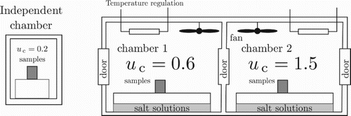
3. Experimental facility
The test facility used to carry out the experiment is illustrated in Figure . It is composed of two connected climatic chambers. The temperature of each chamber is controlled independently with a thermostatically controlled water bath allowing water to recirculate in a heat exchanger. The relative humidity is kept fixed using saturated salt solutions of and
. Relative humidity values in chambers 1 and 2 are fixed to
and
, respectively. Two door locks, at each side, allow the operator to insert or remove samples to minimize system disturbances. They enable easy and instantaneous change in humidity boundary conditions for the samples while passing from one chamber to another. Another climatic chamber is also available used to initially condition materials at
.
Figure 2. Illustration of the RH-box experimental facility.
The temperature and relative humidity fields are measured within the samples with wireless sensors from the HygroPuce range (Waranet industry). The accuracy is for the relative humidity and
for the temperature and the dimensions are
thickness and
diameter, as illustrated in Figure (a). The sensors are placed within the material by cutting the samples. The total uncertainty on the measurement of relative humidity can be evaluated considering the propagation of the uncertainty due to sensor measurement and due to their location. In [Citation23], the total uncertainty on the measurement has been evaluated to
.
Figure 3. Sensors of relative humidity and temperature (a) and wood fibre samples (b) with white acrylic seal and with aluminium tape.
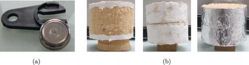
The material investigated is the wood fibre, which properties have been determined in [Citation23,Citation33] and are shown in its dimensionless form in Table . The reference parameter used to compute the unitless parameters is ,
,
and
. It constitutes a priori information on the unknown parameters
,
and
. The samples are cylindrical, with a
diameter and
thickness in order to avoid border effects and to minimize perturbations by sensors placed within the sample. Moreover, to ensure unidimensional moisture transfer and a null flux condition at x=1, the samples are covered with aluminium tape and glued on a white acrylic seal, as illustrated in Figure (b). The convective moisture transport coefficient at x=0 has been estimated experimentally in [Citation23,Citation48]. The corresponding Biot number is reported in Table .
Table 1. A priori dimensionless material properties of wood fibre from [Citation23,Citation33].
Finally, the experimental facility is used to submit the samples to a single or multiple steps of relative humidity. For a single step, the boundary conditions are defined as:
For the case of multiple steps, we set:
where the initial condition belongs to
, the climatic chamber boundary condition
and the duration of the step
. A total of 20 designs are possible for providing measurements to estimate the unknown parameters
,
and
. A synthesis of the possible designs is provided in Table . It should be noted that, according to the reference parameters, unitless values u=0.2, u=0.66, u=1.5 correspond to
,
and
, respectively.
Table 2. Possible designs according to the experimental facility.
4. Searching the OED
4.1. Estimation of one parameter
This section focuses on the estimation of one parameter within ,
or
with experiments coming from single- or multiple-step designs. It should be noted that by estimating parameter
, the complete sorption isotherm curve is defined, according to the dimensionless quantities defined in Section 2.2. The equations to compute the sensitivity functions are given in Appendix 1. In addition, the demonstration of structural identifiability of the three parameters is provided in Appendix 2.
4.1.1. Single step
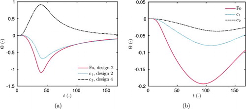
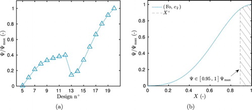
Figure (a) gives the variation of the criterion Ψ for the four single-step designs. For the estimation of parameters or
, the criterion reaches its maximal value for design 2, corresponding to a step from
to
. For parameter
, the design 4 is the optimal one. It can be noted that, for parameter
, the relative criterion Ψ attains
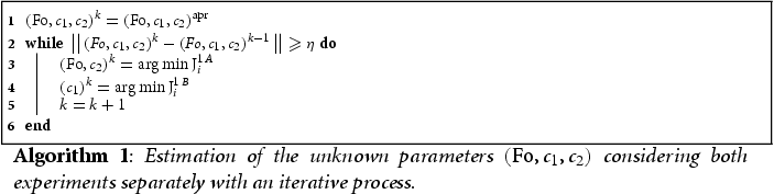
for the design 4. It could be an interesting alternative to estimate this parameter. The variation of the criterion is related to the sensitivity function of each parameter. As noticed in Figure (a,b), functions Θ have higher magnitudes of variation for the OED. The variation of Ψ as a function of the sensor location X is shown in Figure (b) for the OED. The optimal sensor location is at the boundary of the material opposite from the perturbations. If required for practical purpose, the sensor can be placed in the interval
, ensuring to reach
of the criterion Ψ. Results have similar tendencies for the three parameters.
Figure 4. Variation of the criterion Ψ for the four possible single-step designs (a) and as a function of the sensor position X for the OED (b), in the case of estimating one parameter.
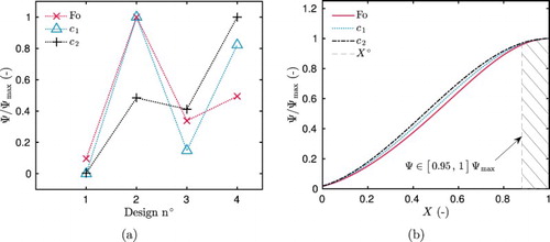
Figure 5. Sensitivity coefficients Θ for parameters ,
and
for the OED (a) and for design 1 (b) (
).
4.1.2. Multiple steps
Figure (a) shows the variation of the relative criterion Ψ for the designs considering multiple steps of relative humidity. It increases with the duration τ of the steps. Thus, for the group of designs 5–12 and the groups 13 –20, the criteria reach their maximum for designs 12 and 20, respectively, corresponding to the step duration . The groups 5–12 correspond to a multiple step
,
,
. For them, the criterion does not attain
of the maximal criteria. Therefore, it is preferable to choose among designs 18–20, with a multiple step
,
,
, and a duration
to estimate the parameters. Figure (a–d) compares the sensitivity function of each parameter for three different designs. The quantity Θ has higher magnitude of variation for the OED than for the others. Moreover, for the design 5, the duration of the step is so short that there is almost no variation on the sensitivity when occurring the first step for
. As for the previous case, the optimal sensor position is
.
Figure 6. Variation of the criterion Ψ for the 16 possible designs (a) and as a function of the sensor position X for the OED (b), in the case of estimating one parameter.
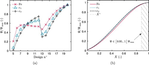
Figure 7. Sensitivity coefficients Θ for parameters ,
and
for the OED (design 20) (a), design 12 (b), design 5 (c) and design 13 (d) (
).
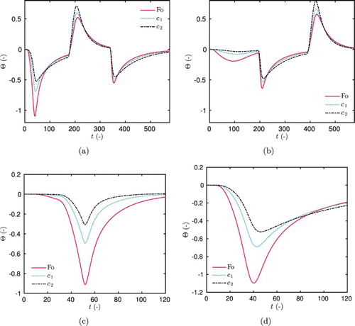
Figure 8. Variation of the criterion Ψ for the four possible designs of single step of relative humidity (a) and as a function of the sensor position X for the OED (b), in the case of estimating the couple of parameters .
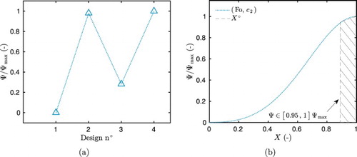
Figure 9. Variation of the criterion Ψ for the 16 possible designs of multiple steps of relative humidity (a) and as a function of the sensor position X for the OED (b), in the case of estimating the couple of parameters .
4.2. Estimation of several parameters
The issue is now to estimate two or three parameters defining the moisture capacity ,
and
. First of all, it is important to notice in Figures and that the sensitivity function Θ of the parameters has a strong correlation. The interval of variation of the correlation coefficients for all the designs is:
Therefore, the estimation of the three parameters at the same time using only one experiment might be a difficult task. In addition, over all the possible designs, the couple of parameters
is the one with the lower correlation. Therefore, the OED search will only consider their estimation.
4.2.1. Single step
Figure (a) gives the variation of the criterion Ψ for the four possible designs, considering a single step of relative humidity. The OED is reached for design 4. However, the design 2 represents an interesting alternative as more than of the maximum criterion is reached. The sensor should be placed between
.
4.2.2. Multiple steps
The variation of the criterion Ψ for the 16 designs is shown in Figure . It increases with the duration of the steps τ. The OED is reached for the design considering a multiple step ,
,
and
, with a duration
. As for the previous case, the OED is defined for a sensor placed near the boundary of the material
.
5. Estimation of the unknown parameters
5.1. Methodology
As mentioned before, the sensitivity functions of parameters ,
and
are strongly correlated and the estimation of the three parameters using one single experiment might be a laborious task. To answer this issue, a single step, referenced as experiment A, will be used for the estimation of the parameter
and a multiple step, referenced as experiment B, for the parameters
, which sensitivity functions are less correlated. According to the results of the OED, the sensor is placed near the border
. For the boundary conditions, the single step will be operated from
to
(design 2 from Table ). The OED multiple step is defined as
,
,
,
and a duration of each step
(design 20 from Table ).
To estimate the unknown parameters, the following cost function is defined by minimizing the residual between the experimental data and the numerical results of the direct model:
Several expressions of the cost function are tested. The subscript i denotes the norm used for the cost function : i=2 stands for the standard discrete
norm while
for the
(uniform) norm. The upper-script
implies that both experiments are considered separately. The single step is used for estimating parameter
and the multiple-step experiment for the parameters
. In such case, there is a cost function according to each experiment:
The estimation of the unknown parameters proceeds in an iterative approach as described in the Algorithm 1. In this case, a tolerance has been chosen.
When , both experiments of single and multiple steps are considered at the same time, without any distinction. For
, parameters
are estimated at once. An additional test, for
is carried by considering both experiments to estimate all the material properties parameters
. Thus, in these cases, the cost functions are defined as:
for
, and for
:
Table synthesizes all tests performed according to the definition of the cost function . The cost function
is minimized using function fmincon in the MatlabTM environment, providing an efficient interior-point algorithm with constraint on the unknown parameters [Citation49]. Here, the box-type constraints are defined with upper and lower bound for the parameters:
where the upper-scripts ° and
denote the estimated and a priori values of the parameters, respectively. The bounds have been defined by performing previous tests and analysing the parameter impact on the calibration.
Table 3. Synthesis of the tests carried out with the expression of the cost function.
In order to quantify the quality of measured data, we estimate the noise inherent to any real physical measurement. By assuming that the noise is centred Gaussian (i.e.
), linear and additive, its variance
can be thus estimated. Moreover, we assume that the underlying signal is smooth. In order to extract the noise component, the signal is approximated locally by a low-order polynomial representing the trend. Then, the trend is removed by using a special filter, leaving us with the pure noise content, which can be further analysed using the standard statistical techniques. For the considered data, the variance equals:
The noise variance does not necessarily correspond to the measurement accuracy. This measure provides a lower bound of this error, i.e. the accuracy cannot be lower than the noise present in the measurement.
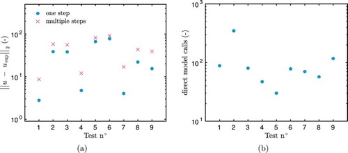
5.2. Results
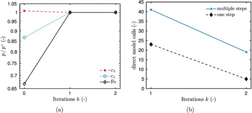
Figure (a) shows the variation of the residual between the measured data and the numerical results for different tests performed. The residual is minimized for tests 1, 4 and 7, corresponding to the involving considering the Euclidean norm for the computation of the cost functions. The tendencies are similar for both experiments. It can be noted that the residual is lower when estimating only three parameters and not all the parameters of the material properties. Figure (b) provides the number of computations of the direct problem. As expected, the tests 1–3, considering both experiments separately, require a few more computations of the direct problem, due to the iterative procedure. Globally, the algorithm requires less than 100 computations, which is extremely low compared to stochastic approaches. For instance in [Citation18],
computations are necessary to estimate the thermal conductivity of two materials by solving an inverse heat transfer problem.
Figure 10. Residual between the measured data and numerical results for both experiments (a) and number of computations of the direct problem (b) for the different definition of the cost function .
The comparison of the measured data and numerical results is illustrated in Figure (a) for the one-step experiment. Figure (b) shows it for the multiple-step procedure, for the case 20. Results of the numerical model are provided for the a priori and estimated three parameters. As mentioned in the Introduction, the numerical model with a priori parameters predicts values lower than those obtained from experiments during the moisture adsorption and greater than them along the desorption processes. With the calibrated model,
i.e. with the estimated parameters, there is a better agreement between the numerical results and the experimental data. Figure (c,d) shows the residual. It is uncorrelated, highlighting a satisfactory estimation of the parameters. Nevertheless, it can be noted that some discrepancies remain between the experimental data and the numerical results. This can be specifically observed at , in Figure (b,d), for which some explanations are possible. First, the mathematical model may fail in representing the physical phenomenon. Some assumptions such as isothermal conditions, unidimensional transport and constant velocity might contribute to the differences observed between experimental and numerical results. Although the experiment has been conceived to be isothermal, slight variations in the temperature field occur due to mechanisms of phase change that may affect the profile of vapour pressure, which is highly temperature-dependent. An important assumption, very often considered in literature, is the disregard of the hysteresis phenomenon, which may considerably affect the results. This issue can be noted in Figure (b) for
. A good agreement is noted during the adsorption process
, since the coefficients have been estimated for a similar experiment. However, during the desorption process, the field u is underestimated by the numerical predictions. On the other hand, despite the low relative humidity uncertainty, other uncertainties appear such as the interference of sensors on the moisture transfer through the sample, contact resistances and no perfect impermeabilization. Another possible explanation is associated to the parametrization of the material properties that can be improved. An interesting alternative could be to search for time varying parameters by adding a regularization term in the cost function
. The convergence of the parameter estimation is shown in Figure (a). On the contrary to parameters
and
, the a priori values of
are not far from the estimated one. After one iteration, the algorithm almost estimates the parameters. The number of computations of the direct model for test 1 is given in Figure (b). Only two global iterations are required to compute the solution of the inverse problem. More computations are required at the first iteration as the unknown parameters are more distant from the estimated optimal ones.
Figure 11. Comparison of the numerical results with the experimental data (a–b) and their confidence interval for the single-step (a) and the multiple-step (b) experiments (test 1). Comparison of the residual for the single-step (c) and multiple-step (d) experiments.
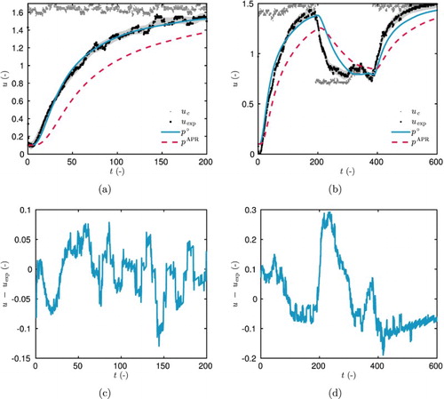
Figure 12. Convergence of the parameter estimation, for the test 1 as a function of the number of iterations (a) and number of computations of the direct model (b).
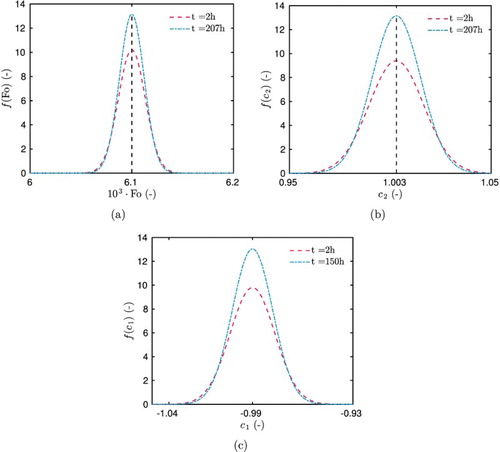
The computation of the sensitivity functions of the parameters to be estimated enables to approximate their probability density functions. The error is assumed as a normal distribution with its standard deviation
computed by adding the ones due to uncertainty and to the noise:
Thus, the probability distribution is computed for different times as illustrated in Figure . As reported in Figure (a), the sensitivity function of parameters and
is maximum and minimum at t=207 and
, respectively. It explains why the probability function is maximum at t=207 for these parameters. Similar results can be observed when comparing the sensitivity function of parameter
in Figure (a) and the probability function in Figure (c).
Figure 13. Probability density function approximated for the estimated parameters, computed using the sensitivity of single-step (c) and a multiple-step (a–b) experiments.
6. Accounting for hysteresis
As mentioned in the description of the physical model, the hysteresis effects are not considered in the sorption capacity of the material. This assumption impacts the comparison between numerical and experimental observations, particularly for the cases of multiple steps of relative humidity (Figure (b)). In this section, the physical model is changed to revise this assumption, which is commonly considered.
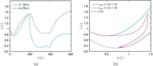
6.1. Model for hysteresis
The hysteresis impacts the sorption curve and consequently on the moisture capacity coefficient c defined in Equation (Equation5
(6)
(6) ). To account for hysteresis, several model are available in literature as proposed in [Citation50] or in [Citation51]. Recently, in [Citation52], a new model of hysteresis has been proposed and validated using experimental data. This model is referred as a smoothed bang–bang model in control literature. It enables intermediary sorption states between the main adsorption
and desorption
curves illustrated in Figure (b). The coefficient c is computed using the following dimensionless differential equation:
(21)
(21) As for the previous case, these two properties are assumed to be second-degree polynomials of the relative humidity:
It should be noted here that the dimensionless coefficient
is defined as
. The coefficient β is a numerical parameter, controlling the transition velocity between the two curves. The function
is defined as:
The mathematical model of moisture transfer is now defined by a system of one partial differential equation coupled with an ordinary differential equation:
(22)
(22)
(23)
(23)
associated with initial and boundary conditions.
The issue is now to estimate the five coefficients of the adsorption and desorption curves . It should be noted that the demonstration of structural identifiability of the five parameters is provided in Appendix 2. When searching the OED, one need to compute the partial derivative of u according to each coefficient
. Since the model is now composed of two differential equations, for each coefficients, two sensitivity functions have to be computed. For instance, for the coefficient
, it is required to compute:
From a mathematical point of view, the computation of is not possible since the function
is not differentiable in the classical sense for x=0. It is differentiable in the sense of distributions. Therefore, a regularized version of the hysteresis model (Equation18
(21)
(21) ):
where the function
is defined as:
with δ a sufficiently large real parameter. In this study, the following value is taken
. A numerical validation of the regularized hysteresis model is provided in Appendix 3.
6.2. Searching the OED
The OED is now searched among the experimental designs described in Section 3 for both single and multiple steps. The issue is to estimate one or several parameters among the five coefficients . For this, the sensitivity functions
and
are computed using central finite-difference and a Runge–Kutta approach provided by ode45 solver in MatlabTM [Citation53]. The equations to compute the sensitivity functions are given in Appendix 1.
First, the OED is searched using the adsorption coefficients estimated in Section 5 and the desorption coefficients obtained from literature [Citation33]:
The Fourier number corresponds to the estimated one in Section 5 and equals . The investigations are performed for both the single and multiple steps of relative humidity, identified in Table . For the sake of compactness, the results are illustrated only for the multiple-step experiments. By improving the model with hysteresis effects, one has to compute the sensitivity coefficients for both equations (Equation19a
(22)
(22) ) and (Equation19b
(23)
(23) ). The sensitivity coefficients
and
are shown in Figures (a,c) for the adsorption coefficients
and
. The variation of the sensitivity coefficients follows the changes in the boundary conditions
. The design 12 corresponds to the OED for each parameter to be estimated, as shown in Figure . On the contrary to the results obtained in Section 4, the design 20 does not allow to estimate the unknown parameters with accuracy. The influence of including the hysteresis effects in the mathematical model can be remarked in the determination of the OED. Indeed, by comparing Figures and , it can be noticed that the sensitivity coefficients
and
have larger magnitudes for the OED than for the design 20. For multiple-step experiments, a strong correlation is observed between the five coefficients
:
indicating that it is not possible to estimate more than two parameters of the model for such experiments. For single case experiments, the correlation is lower:
Thus, for this case, it is possible to estimate a couple of two parameters among or
. The OED results are synthesized in Table . For all experiments, the sensor should be located at the bottom of the material, near the impermeable face. The designs 2 (
to
) and 12 (
,
,
,
and a duration of each step
) provide the highest accuracy to estimate the parameters. Due to high correlation between the coefficients, it is important to note that it is not possible to estimate all five coefficients considering the possible designs described in Table . If one aims at estimating the five coefficients, additional designs have to be planned with the experimental facility, including for instance other levels of relative humidity.
Figure 14. Variation of the criterion Ψ for the 16 possible designs for the adsorption coefficients (a) and the desorption coefficients (b).
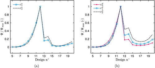
Figure 15. Sensitivity coefficients (a,b) and
(c,d) for the OED (design 12,
).
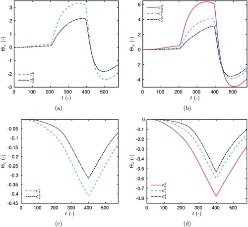
Figure 16. Sensitivity coefficients (a,b) and
(c,d) for the design 20, (
).
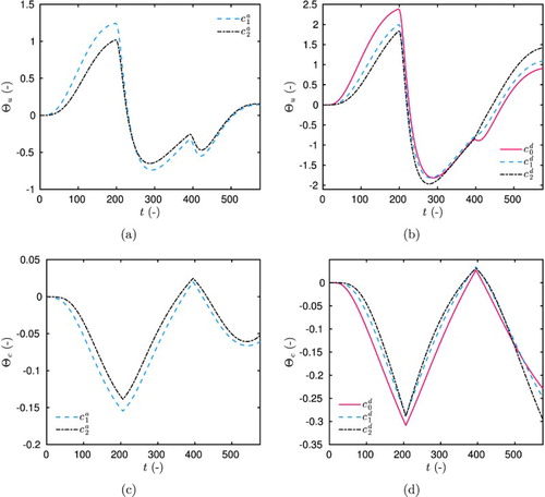
Table 4. Synthesis of OED for the estimation of one or several parameters when the model account for hysteresis.
6.3. Comparing the numerical results with the experimental observations
Previous section aimed at illustrating the possibility of searching the OED with an improved model that includes the hysteresis effects. Since it is rather difficult to estimate the five coefficients due to strong correlations of the sensitivity functions, the purpose is now to show the influence of taking into account the hysteresis effects in the model. It should be noted that the regularized model is not needed so that the normal hysteresis model given by Equation (Equation19b(23)
(23) ) is used for the present case study. To avoid stability restrictions, an implicit–explicit numerical scheme, detailed in Appendix 4, is employed to compute numerically the solution.
The numerical predictions are compared with the experimental observations for the multiple-step experiment (design 20). The adsorption coefficients, estimated in Section 5, are used together with the desorption coefficients obtained from literature [Citation33]. The Fourier number equals and the other parameters have the same numerical value as the ones mentioned in Section 5. Figure (a) shows the comparison between the numerical predictions and the experimental data. The results from the physical model including the hysteresis effects are more satisfactory. Indeed, the residual is lower for this model than for the model without hysteresis, as shown in Figure (b). Particularly, the importance of the hysteresis can be noted for the desorption phase
and the second adsorption phase
. The solution of Equation (Equation19b
(23)
(23) ) enables to compute the time evolution of the sorption coefficient c as illustrated in Figure (a). It is compared with the function
where u is computed using the model without hysteresis given by Equation (Equation12
(14)
(14) ). The time variation of the coefficients is similar for the first adsorption part corresponding to
. Indeed, for this period, the computed sorption coefficient equals the adsorption curve as noticed in Figure (b). After this period, the coefficient computed with the hysteresis model decreases comparing to the one without hysteresis and oscillates between the adsorption and desorption curves as shown in Figure (b).
Figure 17. Comparison of the numerical results with the experimental data (a) and their residual (b).
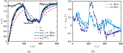
Figure 18. Variation of the sorption coefficient c according to time (a) and according to the computed field u (b).
7. Final remarks
7.1. Conclusion
In the context of building physics, inverse problems are encountered to estimate moisture-dependent hygrothermal properties of porous materials, using measurements associated to heat and moisture transport. Two applications are distinguished. In the first case, concerning the diagnosis of existing building walls, there is a few a priori estimation of material properties. Moreover, measurements must be non-intrusive and non-destructive. In the second case, measurements are performed in the laboratory to calibrate the numerical model with the experimental data. This article is encompassed in these conditions, focused on the estimation of moisture sorption isotherm coefficients of a wood fibre material.
First, the OED methodology has been described and used for searching the OED, ensuring to provide the best accuracy of the identification method for the parameter estimation. The approach is based on the sensitivity functions of the unknown parameters, enabling to determine sensor location within the material and boundary conditions, according to an existing facility among 20 possible designs. It has been carried out considering a priori values of the unknown parameters. The facility allows to submit material to relative humidity steps on one surface, being all others moisture impermeable. Results have enhanced two designs: (i) single step of relative humidity from to
and (ii) multiple steps of relative humidity
, with a duration period of 8 days for each step. For each design, the sensor has to be placed as close as possible to the impermeable boundary.
Then, experimental data have been provided according to the OED results for the two selected designs. The parameter estimation has been conducted by minimizing a cost function between the experimental data and the numerical results. The estimation has been accomplished using an interior point algorithm. Nine tests have been performed for the definition of the cost function . The
and
have been evaluated. Two series of tests aimed at estimating the three parameters using both experiments at the same time or separately with an iterative algorithm. The third series intended to estimate all five parameters of the material properties. Results have shown that the
norm provided better results of the parameter estimation problem. Moreover, it was better to consider both experiments separately to estimate only three parameters of the problem. Within this approach, the algorithm requires only two iterations to compute the solution with less than 100 computations of the direct model. This approach has a really low computational cost compared to stochastic approaches, needing an order of
computations for similar problems. Another advantage of this approach is to use the sensitivity functions, computed during the search of the OED, to provide an approximation of the probability distribution function of the estimated parameters at a lower computational cost.
As highlighted in Section 5, with the estimated parameters, a better agreement between the numerical model and the experimental data is observed. However, the importance of hysteresis effects were highlighted. Particularly, when cycles of desorption–adsorption processes take place, some discrepancies remain between experimental data and numerical predictions. Therefore, a new mathematical model has been proposed to take into account the hysteresis effects on the sorption coefficients. A second differential equation has been added and increased to five the number of coefficients to be estimated. Two coefficients correspond to the adsorption curve and three to the desorption one. A regularized version of the hysteresis model was proposed to have continuous differentiable functions and, therefore, to be able to compute the sensitivity coefficients. Then, the OED was explored by computing the sensitivity coefficients of the five parameters of a family of scanning curves of adsorption and desorption processes. This clearly highlighted the possibility of including the hysteresis effects in the OED approach. The results draw attention to two designs: (i) a single step of relative humidity from to
and (ii) multiple steps of relative humidity
, with a 8-day time period for each step. The sensors have to be placed near the impermeable boundary.
Finally, the numerical predictions, considering the hysteresis phenomenon, have been compared with the experimental observations of a multiple-step design. An efficient implicit–explicit numerical scheme was proposed to compute the solution of the hysteretic model. The parameters of this model correspond to the estimated ones in Section 5 for the adsorption curve and to the a priori ones provided in the literature. The comparison has shown that the discrepancies are reduced, fitting better experimental data. During the simulation, the computed sorption coefficients oscillated between the ones from the main adsorption and desorption curves.
7.2. Outlooks and open-problems
An interesting perspective of improvement concerns the assumptions related to the moisture sorption isotherm coefficients . A parametrization was previously defined
and the parameter estimation problem aimed at identifying coefficients
,
(and
). An ambitious outlook could aim at estimating directly the function
, with inspiration from the following studies [Citation54,Citation55].
Disclosure statement
No potential conflict of interest was reported by the authors.
Additional information
Funding
References
- U.S. Energy Information Administration. Annual Energy Outlook 2015, with projections to 2040. Washington: EIA; 2015.
- Woloszyn M, Rode C. Tools for performance simulation of heat, air and moisture conditions of whole buildings. Build Simul. 2008;1(1):5–24. doi: 10.1007/s12273-008-8106-z
- Luikov AV. Heat and mass transfer in capillary-porous bodies. London: Pergamon Press; 1966.
- Mendes N, Ridley I, Lamberts R, et al. Umidus: a PC program for the prediction of heat and mass transfer in porous building elements. International Conference on Building Performance Simulation, Japan; 1999. p. 277–283.
- Mendes N, Philippi PC. A method for predicting heat and moisture transfer through multilayered walls based on temperature and moisture content gradients. Int J Heat Mass Transf. January 2005;48(1):37–51. doi: 10.1016/j.ijheatmasstransfer.2004.08.011
- Fraunhofer IBP. Wufi. http://www.hoki.ibp.fhg.de/wufi/wufi_frame_e.html2005.
- Sasic Kalagasidis A, Weitzmann P, Nielsen TR, et al. The International Building Physics Toolbox in Simulink. Energy Build. June 2007;39(6):665–674. doi: 10.1016/j.enbuild.2006.10.007
- Mendes N, Chhay M, Berger J, et al. Numerical methods for diffusion phenomena in building physics. Curitiba: PUC-Press; 2016.
- Mendes N, Philippi PC. Multitridiagonal-matrix algorithm for coupled heat transfer in porous media: Stability analysis and computational performance. J Porous Media. 2004;7(3):193–212. doi: 10.1615/JPorMedia.v7.i3.40
- BC Bauklimatik Dresden Simulation program for the calculation of coupled heat, moisture, air, pollutant, and salt transport. http://www.bauklimatik-dresden.de/delphin/index.php?aLa=en2011.
- Rouchier S, Woloszyn M, Foray G, et al. Influence of concrete fracture on the rain infiltration and thermal performance of building facades. Int J Heat Mass Transf. 2013;61:340–352. doi: 10.1016/j.ijheatmasstransfer.2013.02.013
- Janssen H, Blocken B, Carmeliet J. Conservative modelling of the moisture and heat transfer in building components under atmospheric excitation. Int J Heat Mass Transf. 2007;50(5–6):1128–1140. doi: 10.1016/j.ijheatmasstransfer.2006.06.048
- Gasparin S, Berger J, Dutykh D, et al.Stable explicit schemes for simulation of nonlinear moisture transfer in porous materials. J Building Performance Simul. 2018;11:129–144. doi: 10.1080/19401493.2017.1298669
- Gasparin S, Berger J, Dutykh D, et al. An improved explicit scheme for whole-building hygrothermal simulation. Building Simul. 2018;11:465–481. doi: 10.1007/s12273-017-0419-3
- Berger J, Gasparin S, Dutykh D, et al. Accurate numerical simulation of moisture front in porous material. Build Environ. 2017;118:211–224. doi: 10.1016/j.buildenv.2017.03.016
- Kabanikhin SI. Definitions and examples of inverse ill-posed problems. J Inverse Probl and Ill -posed problems. 2008;16:317–357.
- Kabanikhin SI. Inverse and ill-posed problems: theory and applications. Berlin: Walter De Gruyter; 2011.
- Berger J, Orlande HRB, Mendes N, et al. Bayesian inference for estimating thermal properties of a historic building wall. Build Environ. 2016;106:327–339. doi: 10.1016/j.buildenv.2016.06.037
- Rouchier S, Woloszyn M, Kedowide Y, et al. Identification of the hygrothermal properties of a building envelope material by the covariance matrix adaptation evolution strategy. J Build Perform Simul. 2014;9(1):101–114. doi: 10.1080/19401493.2014.996608
- Nassiopoulos A, Bourquin F. On-site building walls characterization. Numer Heat Transfer Part A – Appl. 2013;63(3):179–200. doi: 10.1080/10407782.2013.730422
- James C, Simonson CJ, Talukdar P, et al. Numerical and experimental data set for benchmarking hygroscopic buffering models. Int J Heat Mass Transf. 2010;53(19–20):3638–3654. doi: 10.1016/j.ijheatmasstransfer.2010.03.039
- Kanevce GH, Kanevce LP, Dulikravich GS, et al. Estimation of thermophysical properties of moist materials under different drying conditions. Inverse Probl Sci Eng. 2005;13(4):341–353. doi: 10.1080/17415970500098485
- Berger J, Busser T, Dutykh D, et al. On the estimation of moisture permeability and advection coefficients of a wood fibre material using the optimal experiment design approach. Experiment Thermal and Fluid Sci. 2018;90.246–259. doi: 10.1016/j.expthermflusci.2017.07.026
- Rouchier S, Busser T, Pailha M, et al. Hygric characterization of wood fiber insulation under uncertainty with dynamic measurements and Markov Chain monte-Carlo algorithm. Build Environ. 2017;114:129–139. doi: 10.1016/j.buildenv.2016.12.012
- Biddulph P, Gori V, Elwell CA, et al. Inferring the thermal resistance and effective thermal mass of a wall using frequent temperature and heat flux measurements. Energy Build. 2014;78:10–16. doi: 10.1016/j.enbuild.2014.04.004
- Dubois S, McGregor F, Evrard A, et al. An inverse modelling approach to estimate the hygric parameters of clay-based masonry during a moisture buffer value test. Build Environ. 2014;81:192–203. doi: 10.1016/j.buildenv.2014.06.018
- Xu X, Wang S. Optimal simplified thermal models of building envelope based on frequency domain regression using genetic algorithm. Energy Build. 2007;39(5):525–536. doi: 10.1016/j.enbuild.2006.06.010
- Czel B, Grof G. Inverse identification of temperature-dependent thermal conductivity via genetic algorithm with cost function-based rearrangement of genes. Int J Heat Mass Transf. 2012;55(15–16):4254–4263. doi: 10.1016/j.ijheatmasstransfer.2012.03.067
- Palomo Del Barrio E. Multidimensional inverse heat conduction problems solution via lagrange theory and model size reduction techniques. Inverse Probl Eng. 2003;11(6):515–539. doi: 10.1080/1068276031000114884
- Berger J, Dutykh D, Mendes N. On the optimal experiment design for heat and moisture parameter estimation. Exp Therm Fluid Sci. 2017;81:109–122. doi: 10.1016/j.expthermflusci.2016.10.008
- Belleudy C, Woloszyn M, Chhay M, et al. A 2D model for coupled heat, air, and moisture transfer through porous media in contact with air channels. Int J Heat Mass Transf. 2016;95:453–465. doi: 10.1016/j.ijheatmasstransfer.2015.12.030
- Delleur JW. The handbook of groundwater engineering. 2nd ed. New York: CRC Press; 2006.
- Rafidiarison H, Rémond R, Mougel E. Dataset for validating 1-d heat and mass transfer models within building walls with hygroscopic materials. Build Environ. 2015;89:356–368. doi: 10.1016/j.buildenv.2015.03.008
- Vololonirina O, Coutand M, Perrin B. Characterization of hygrothermal properties of wood-based products – impact of moisture content and temperature. Constr Build Mater. 2014;63:223–233. doi: 10.1016/j.conbuildmat.2014.04.014
- Necati Ozisik M, Orlande HRB. Inverse heat transfer: fundamentals and applications. New York: CRC Press; 2000.
- Finsterle S. Practical notes on local data-worth analysis. Water Resour Res. 2015;51(12):9904–9924. doi: 10.1002/2015WR017445
- Walter E, Pronzato L. Qualitative and quantitative experiment design for phenomenological models; a survey. Automatica. 1990;26(2):195–213. doi: 10.1016/0005-1098(90)90116-Y
- Nenarokomov AV, Titov DV. Optimal experiment design to estimate the radiative properties of materials. J Quant Spectros Radiat Tran. 2005;93(1–3):313–323. doi: 10.1016/j.jqsrt.2004.07.036
- Artyukhin EA, Budnik SA. Optimal planning of measurements in numerical experiment determination of the characteristics of a heat flux. J Eng Phys. 1985;49(6):1453–1458. doi: 10.1007/BF00871299
- Beck JV, Arnold KJ. Parameter estimation in engineering and science. New York: John Wiley and Sons; 1977.
- Wouwer AV, Point N, Porteman S, et al. An approach to the selection of optimal sensor locations in distributed parameter systems. J Process Control. 2005;10(4):291–300. doi: 10.1016/S0959-1524(99)00048-7
- Fadale TD, Nenarokomov AV, Emery AF. Two approaches to optimal sensor locations. ASME J Heat Trans. 1998;117(2):373–379. doi: 10.1115/1.2822532
- Emery AF, Nenarokomov AV. Optimal experiment design. Meas Sci Technol. 1998;9(6):864.876 doi: 10.1088/0957-0233/9/6/003
- Anderson ML, Bangerth W, Carey GF. Analysis of parameter sensitivity and experimental design for a class of nonlinear partial differential equations. Int J Numer Methods Fluids. 2005;48(6):583–605. doi: 10.1002/fld.938
- Alifanov OM, Artyukhin EA, Rumyantsev SV. Extreme methods for solving ill-posed problems with applications to inverse heat transfer problems. New York: Begellhouse; 1995.
- Karalashvili M, Marquardt W, Mhamdi A. Optimal experimental design for identification of transport coefficient models in convection–diffusion equations. Comput Chem Eng. 2015;80:101–113. doi: 10.1016/j.compchemeng.2015.04.036
- Ucinski D. Optimal measurement methods for distributed parameter system identification. New York: CRC Press; 2004.
- Busser T, Piot A, Pailha M, et al. From materials properties to modelling hygrothermal transfers of highly hygroscopic walls. Dresden: CESBP; September 2016 .
- Byrd RH, Gilbert JC, Nocedal J. A trust region method based on interior-point techniques for nonlinear programming. Math Program. 2000;89(1):149–185. doi: 10.1007/PL00011391
- Mualem Y, Beriozkin A. General scaling rules of the hysteretic water retention function based on Mualem's domain theory. Eur J Soil Sci. 2009;60(4):652–661. doi: 10.1111/j.1365-2389.2009.01130.x
- Derluyn H, Derome D, Carmeliet J, et al. Hysteretic moisture behavior of concrete: modeling and analysis. Cement and Concrete Research. 2012;42(10):1379–1388. doi: 10.1016/j.cemconres.2012.06.010
- Berger J, Gasparin S, Dutykh D, et al. On the solution of coupled heat and moisture transport in porous material. Transp Porous Media. 2018;121:665–702. doi: 10.1007/s11242-017-0980-3
- Shampine LF, Reichelt MW. The MATLAB ODE suite. SIAM J Sci Comput. 1997;18(–):1–22. doi: 10.1137/S1064827594276424
- Koptyug IV, Kabanikhin SI, Iskakov KT, et al.A quantitative NMR imaging study of mass transport in porous solids during drying. Chem Eng Sci. 2000;55(9):1559–1571. doi: 10.1016/S0009-2509(99)00404-2
- Kabanikhin SI, Hasanov A, Penenko AV. A gradient descent method for solving an inverse coefficient heat conduction problem. Numer Anal Appl. 2008;1(1):34–45. doi: 10.1134/S1995423908010047
- Walter E, Lecourtier Y. Global approaches to identifiability testing for linear and nonlinear state space models. Math Comput Simul. 1982;24(6):472–482. doi: 10.1016/0378-4754(82)90645-0
Appendices
A.1. Appendix 1. Equations for the computation of the sensitivity coefficients
This section provides the equations derived analytically from the mathematical model (Equation (Equation12(14)
(14) )), to compute the sensitivity coefficients.
A.1.1 Model without hysteresis
The sensitivity coefficients are denoted as follows:
For the sake of clarity, the superscript is omitted. The sensitivity coefficients verified the following equations. For
:
For
:
and for
:
A.1.2 Model with hysteresis
The model with hysteresis includes two differential equations, recalled here:
Therefore, two sensitivity coefficients have to be computed. The differential equations for
and
are:
For
and
:
For
and
:
For
and
:
For
and
:
The function
is the regularized Dirac function:
Figure A1. Time variation of the field u (a) and of the sorption capacity c (b) for the model with hysteresis and the regularised one.
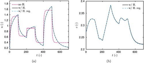
Figure A2. Variation of the sorption capacity c with the field u (a) according to the case study. Time variation of the error (b) for the fields u and c between the model with hysteresis and the regularised one.
A.2 Appendix 2. Proving the structural identifiability of the parameters
This section aims at justifying the identifiability of the unknown parameters for both model with and without hysteresis. We recall that a parameter P is Structurally Globally Identifiable (SGI) if the following condition is satisfied [Citation56]:
where y is the response of the model depending on parameter P.
A.2.2 Model without hysteresis
First, the SGI is demonstrated for the estimation of parameters in the model (Equation12
(14)
(14) ), recalled here without the superscript
:
(24)
(24) It is assumed that u is observable. So as to prove identifiability, it is assumed that another set of parameters, denoted with a superscript
, holds:
(25)
(25) If
then
and
. Thus, from Equations (EquationA1
(24)
(24) ) and (EquationA2
(25)
(25) ) we have:
and
Since
and
, it follows that
Therefore, parameters
are SGI for the model without hysteresis.
A.2.3 Model with hysteresis
Now, the SGI for the five parameters is demonstrated for the model with hysteresis. For this, Equation (Equation18
(21)
(21) ) is recalled omitting the superscript
:
Similarly, to prove the identifiability, another set of parameters is assumed:
It is assumed that
,
and then
. Using the symbolic code MapleTM, by expansion it can be demonstrated that:
and that the parameters are SGI.
A.3 Appendix 3. Numerical validation of the regularized hysteresis model
A computation using the regularized hysteresis model is carried out:
where the numerical values of the coefficients are:
The initial and boundary conditions are defined in Equation (Equation12
(14)
(14) ) with the following numerical values:
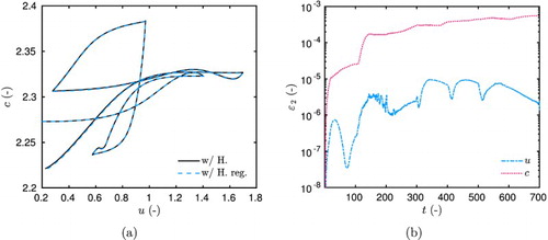
The case study is similar to the experimental designs investigated in this work. The simulation time horizon is t=700. The time variations of the field u are given in Figure (a). The results of the regularized and non-regularized model are compared to the model with no-hysteresis, considering only the adsorption curve. The importance of the hysteresis in the time variations of u can be noted. Figure (b) shows the time variation of c by computation of its differential equation. The variations of the sorption coefficient c with the computed values of u are shown in Figure (a). In both Figures (b) and (a), a perfect agreement is observed between the regularized and non-regularized models. Moreover, as noticed in Figure (b), the
error of the fields u and c, computed between the regularized and non-regularized models, scales with
and
, respectively. The agreement between the results of the two models is very satisfactory, validating the implementation of the regularized hysteretic model.
A.4 Appendix 4. Implicit–explicit numerical scheme for the hysteresis model
To relax stability restriction, an implicit–explicit numerical scheme is used to compute the solution of the hysteresis model:
(26)
(26) For the sake of clarity, the ⋆ superscript have been omitted. A uniform discretisation is considered for time intervals. The discretisation parameter is denoted using
for the time. The discrete values of function
are denoted by
with
.
When , Equation (EquationA3
(26)
(26) ) is discretized according to:
which gives the explicit expression of
:
Similarly, when , Equation (EquationA3
(26)
(26) ) is discretized according to:
to obtain the explicit expression of
:
This numerical scheme provides robust and stable results as already shown in Figures and .