
 ?Mathematical formulae have been encoded as MathML and are displayed in this HTML version using MathJax in order to improve their display. Uncheck the box to turn MathJax off. This feature requires Javascript. Click on a formula to zoom.
ABSTRACT
This paper presents an efficient alternating method for image deblurring and denoising, it is based on our new model with TV norm to denoise the deblurred image which is penalized by norm of the framelet transform. Our combinational algorithm performs deblurring and denoising alternately. We apply the proximity algorithm to solve the TV regularization for denoising part, and the mean doubly augmented Lagrangian (MDAL) method is used to solve
minimization in the analysis-based sparsity for the deblurring part. Experimental results show that the proposed alternating minimization method is robust for a different type of blur and noise. We also do some comparisons with related existing methods to demonstrate that our method has a more significant effect.
1. Introduction
Digital image restoration is an important problem in image processing which is widely applied to medical and astronomical imaging, film restoration, image and video coding [Citation1–8] and so on. The image restoration task can be formulated as a linear inverse problem:
(1)
(1) where
is the observed degraded image,
represents a spatial-invariant blur matrix which is constructed by the blur kernel,
is the original image to be restored,
denotes an additive Gaussian white noise with some kind of deviation σ.
To obtain a reasonable approximated solution u of this problem, various regularization-based methods have been proposed in the past decades. One of the most popular is the Rudin–Osher–Fatemi (ROF) model with total variation (TV) regularization, proposed by Rudin, Osher and Fatemi [Citation9]. A discrete version of the unconstrained TV regularization is given by
(2)
(2) where
denotes the Euclidean norm, α is a positive regularization parameter which measures the trade-off between a good fit and a regularized solution, and
is the TV regularization term. When A is an identity matrix, the ROF model produces the denoising case. The model is initially solved by the partial differential equation, which has high computational complexity.
Difficulty in minimizing the functional appearing in (Equation2(2)
(2) ) lies in the nondifferentiability of the total variation semi-norm and the large dimension of the underlying images. A number of numerical methods have been proposed to address these issues. The most popular is direct optimization [Citation9–11] by solving the associated Euler-Lagrangian equations [Citation12–16]. Other methods including subgradient descents, second-order cone programming, interior point methods, graph-based approaches, Nesterov's first-order explicit schemes [Citation17–21], the split Bregman iteration methods and its variations [Citation22–25], which introduces an intermediate variable to make the ROF model separable so that the minimization of the resulting functional is easier to solve.
Micchelli, Shen and Xu [Citation26] proposed the proximity algorithm to solve the ROF model for image denosing which is simple and efficient. The total-variation can be viewed as the composition of a convex function (the norm for the anisotropic total-variation or the
norm for the isotropic total-variation) with a linear transformation, then use the fixed-point algorithm for computing the proximity operator of the composition of the convex function with a linear transformation.
A fast TV minimization method is proposed by Huang, Ng and Wen [Citation27] for image restoration. They modified the above unconstrained TV problem (Equation2(2)
(2) ) as follow:
(3)
(3) where
are positive regularization parameters. In (Equation3
(3)
(3) ), we can interpret the TV minimization scheme to denoise the deblurred image u. The TV norm for the image restoration process is able to preserve edges very well.
In [Citation28], Dong and Zhang proposed a framelet-based method which the image term u had a sparse representation in some redundant transform domain, and penalized by norm which is widely researched in [Citation29–33]. Synthesis-based sparsity and analysis-based sparsity priors are two famous sparse approximations. Because analysis-based approach has a smoother solution than that of synthesis-based approach, the focus of the paper is the analysis-based approach, the detail information about the two sparse representation can be referred to [Citation34,Citation35].
It has been proved in [Citation27] that it is a good idea to bring in auxiliary variable v to denoise and deblur image alternately and use the TV minimization scheme in denoising step. Since the regularization based on the framelet transform has the outstanding performance on image deblurring, we apply the analysis-based approach for the deblurring step. Motivated by the mentality of [Citation27] and the excellent effect of [Citation28], we propose a new optimization model:
(4)
(4) where W is a matrix based on framelet transform, this framelet form tight wavelet frame, detail description can be found in [Citation36],
are positive regularization parameters, α measures the trade-off between a deblurred image u and a denoised image v, λ and
measure the amount of regularization to a deblurring image u and a denoising image v, respectively.
The first advantage of this paper is the new model which alternates deblurring and denoising, our new model bases on TV norm and norm in framelet transform is superior than relative models. The second advantage is designing a combinational algorithm which consists of the mean doubly augmented Lagrangian (MDAL) method and the proximity algorithm. The MDAL method is to solve the
-norm in framelet transform model (Equation4
(4)
(4) ). Because the iterative sequence
obtained by augmented Lagrangian (AL) method can not guarantee the convergence of
, and the doubly augmented Lagrangian (DAL) method may converge slowly and unsteadily, this motivated to consider the mean values of
and
as the outputs of the deblurring step. The proposed algorithm is more effective for image restoration, since it can improve the deblurring and denoising quality, respectively.
The paper is organized as following. In Section 2, we show the detailed implementation of our combinational algorithm based on the MDAL method and proximity algorithm for solving model (Equation4(4)
(4) ), Convergence analysis is given in Section 3, Experimental results are exhibited in Section 4, A brief summary is given in Section 5.
2. Alternating minimization method for deblurring and denoising
In this section, we propose an efficient alternating method for our new model (Equation4(4)
(4) ). Deblurring alternates with Denoising. We use MDAL to solve
regularization based on
the framelet transform for deblurring and employ proximity algorithm based on total variation minimization to denoise the deblurred images, that is deblurring alternates with denoising.
In (Equation4(4)
(4) ), there are two unknown variables, one is the deblurred image u, and the other is the denoised image v. Starting from an initial guess
, we can get a series of
:
such that
(5)
(5)
(6)
(6) with
.
2.1. Deblurring step
The first step of the alternating method is deblurring process which solves the
-norm-based minimization of (Equation5
(5)
(5) ):
(7)
(7) Here we take the effective replacement Wu=d, rewrite minimization (Equation7
(7)
(7) ) as a constrained optimization problem:
(8)
(8) The alternating direction method of multipliers (ADMM) [Citation37] is applied to the augmented Lagrangian (AL) [Citation38] of (Equation7
(7)
(7) ):
(9)
(9) where
controls the weight of the penalty term.
The AL method solving (Equation7(7)
(7) ) can be formulated as iterative steps:
(10)
(10) The AL method can only guarantee the convergence of the dual variable
but not the primal variables
, so the doubly augmented Lagrangian (DAL) is introduced for (Equation7
(7)
(7) ), that is we rewrite the minimizing problem as:
(11)
(11) where
is the functional in (Equation9
(9)
(9) ), the iterative scheme of the DAL method for (Equation11
(11)
(11) ) consists of the following three subproblems:
(12)
(12)
(13)
(13)
(14)
(14) As the subproblem of solving u is differentiable, we solve the following positive definite linear system:
(15)
(15) where
is the conjugate transpose of A.
Then we use fast fourier transform (FFT) to perform the main computation:
here A is usually a matrix of block circulant with circulant blocks when periodic boundary conditions.
The solution of d subproblem can be described as follows:
(16)
(16) where the operator
is a generalized hard-thresholding operator defined componentwisely as
(17)
(17) However, the DAL method may converge slowly and unsteadily, so we use the mean values as the outputs of deblurring, instead the sequence
as
, where
and
. The new sequence
does well converge and satisfies the constraint Wu=d asymptotically, this is the mean doubly augmented Lagrangian method.
2.2. Denoising step
The second step is to denoise the image u generated by the previous deblurring step, this is the minimizer of the optimization problem (Equation6(6)
(6) ):
(18)
(18) Here we employ the proximity algorithm in this denoising step. Total variation can be viewed as the composition of a convex functional,the
norm for the anisotropic total-variation or the
norm for the isotropic total-variation. We use fixed-point algorithm for computing the proximity operator, this method is mathematically sound simple and efficient for solving (Equation19
(18)
(18) ).
So we consider the following isotropic total-variation problem:
(19)
(19) where we denote
. The vector that achieves the minimum in (Equation20
(19)
(19) ), denoted by
, exists and is unique. for convenience we introduce the affine transformation
defined, for all
by
and the operator
given, for a fixed
by
where
satisfies specified condition.
Micchelli, Shen and Xu [Citation26] have proved that the solution of the minimization problem (Equation20(19)
(19) ) is just a fixed point of the operator H which involves the proximity operator of the convex function
and the linear transformation B. Based on the above analysis, we focus on finding the fix-points of the operator H.
Now we consider the Picard iterates of H. For a given initial point , the Picard sequence of H is defined by
The k-averaged operator
of H with
is defined as following:
(20)
(20) To speed up convergence of the iteration, we can also use Gaussian-Seidel variation of the fixed-point algorithm based on the proximity operator for model (Equation20
(19)
(19) ).
Let D denote the matrix defined by the following:
and choose B to be a
matrix given by
(21)
(21) where
is the
identity matrix and the notation ⊗ denotes the Kronecker product.
To present a Gauss-Seidel variation of the fixed-point algorithm, we specialize the above linear transformation T to our current setting. for a given
is defined by
.
By (Equation22(21)
(21) ), we have
(22)
(22) With this notations, we have the following iteration scheme:
(23)
(23) where
(24)
(24) are two components of (Equation23
(22)
(22) ).
In the end, we obtain the minimization of (Equation19(18)
(18) ):
(25)
(25) Similar Gaussian–Seidel variation of the fixed-point algorithm for can be found in [Citation26].
2.3. Summary of the alternating algorithm Fl0pro
The alternating algorithm based on norm in framelet transform for deblurring and proximity algorithm for denoising is named as Fl0pro.
The algorithm is summarized as follows.
3. Convergence analysis
Convergence of iteration for problem (Equation4(4)
(4) ) can be decomposed into two parts, denoising and deblurring, we focus on the existence of optimal solutions to problem (Equation5
(5)
(5) ), the convergence of the fixed-point algorithm for (Equation6
(6)
(6) ) is obvious.
The penalty problem (Equation5(5)
(5) ) can be in general formulated as:
(26)
(26) where the functions
are nondecreasing continuous functions.
For any positive integer k, denote
Given
satisfying the above conditions, the integer L, the sets
,
,
are defined by the following iteration
with initial values
It is well defined and there the following properties are straight forward.
,
where denotes the n-dimensional vector with 0 as its components.
In this way, we can see that in order to establish the existence of optimal solutions to problem (Equation27(26)
(26) ), it suffices to prove the existence of optimal solutions to problem:
for all
.
Similarly as [Citation32], we can prove the following results.
Theorem 1
Given satisfying the above conditions, let
and
for
be defined by the above. Then, the optimal solution set of problem (Equation27
(26)
(26) ) is nonempty for any
. Moreover, we have the following statements:
The optimal value of problem (Equation27
Details are omitted here.
We present the convergence error of DAL method and MDAL method for the image ‘Barbara’ and ‘Kitten’ in Figure , it shows that our MDAL has better performance than DAL.
Figure 1. Relatively errors for the DAL method (dash line) and the MDAL method (solid line).
4. Numerical experiments
In this section, we test four different images which are ‘Barbara’ of size , ‘Kitten’ and ‘Bridge’ of size
, ‘Mandrill’ of size
shown in Figure to show the effectiveness of our proposed method and algorithm for image restoration problems. In addition, we show some blur kernels of our tests added in the figures in Figure . In the following examples, Signal-to-noise ratio (SNR), peak signal-to-noise ratio (PSNR), and structural similarity (SSIM) are used to measure the quality of the restored images, and blurred signal to noise ratio (BSNR) for indicating the noise size of the observed images. They are defined as follows:
where
denote the original image, the observed image, the noise vector added in the test, and the restored image, p is the size of the image, respectively. Mainly, we have the larger SNR, PSNR, SSIM values mean better restored image, and the smaller BSNR value means bigger noise added to the image.
Figure 2. Original images for ‘Barbara’,‘Kitten’,‘Bridge’ and ‘Mandrill’, respectively.
Figure 3. Blur kernels: GB(9,2), AB(9,9), MB(20,0), respectively.
We compare the proposed method which based on norm in framelet transform for deblurring and proximity algorithm for denoising (Fl0pro) with the fast TV method (Fast-TV) in (Equation3
(3)
(3) ), and the MDAL method for
minimization (Fl0) [Citation28]. In all experiments, the stop criterion
is used to terminate iteration. Moreover, we set the maximum iterative number as 100. All the experiments are performed under Windows 7 and MATLAB R2014a running on a desktop (Intel(R) Core(TM) i7-4790 CPU @ 3.60 GHz).
4.1. Parameters selection
In this part, we will mainly discuss some basic guidelines on how to choose the parameters appeared in our algorithms. We determine the best values of parameters from their tested values such that the SNR, PSNR, SSIM values are the relative maximum.
For our proposed model (Equation4(4)
(4) ), we need to consider the parameters
. Here α measures the trade-off between the deblurred image u and the denoised image v, we find for all tested cases that α can be set to be candidate values, i.e.
.
are related to the MDAL method. We choose smaller or larger λ when BSNR is equal to 40 or 30 dB. If the parameter λ is too big, it may result in the restored image over-smooth. If λ is too small, it may induce incompleteness of denoising. μ is only related to the convergence rate of the augmented Lagrangian, setting different values of μ does not change the outcome. The parameter γ controls the regularity of the sequence
, here it has two candidate values
. According to the computational results, the choose of
should satisfy the condition of
, here we choose
. For
, we select
. From our trials, we know that too large
leads to too smooth of denoised image, and too small
may cause noise residue.
4.2. Numerical results
In this part, we present numerical results for three kinds of cases, the noise is the same Gaussian,and the blur is three kinds of different types.
Case 1. Gaussian blur and Gaussian noise
In this section, we demonstrate the efficiency of our proposed method for different images with Gaussian blur and Gaussian noise. We do the comparison of the three algorithms by the SNR, PSNR, SSIM values, number of iterations and CPU running time when the maximum iterative number is the same. Here the Gaussian blur is ,
,
pixels with standard deviation
and the additive Gaussian noise is 40 or 30 dB.
In Table , the ‘Blur/ BSNR’ means that the degraded images have the type and level of blur and the size of noise, the SNR values of the degraded image are showed in the column of ‘Blur/ BSNR’. According to the values we see that the SNR, PSNR, SSIM values of the restored images by the proposed method (Fl0pro) is almost bigger than those by the fast TV method (Fast-TV) in (Equation3(3)
(3) ), and the MDAL method based on
minimization (Fl0). The proposed Fl0pro method is generally much better than Fl0 in computation efficiency, but consumes more running time in seconds and number of iterations than Fast-TV in general.
Table 1. SNR, PSNR(dB), SSIM values, iteration numbers, and CPU time of different methods for the different images corrupted by Gaussian blur and Gaussian noise.
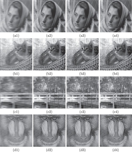
Here we show the image of ‘Barbara’ for GB(5,2)/40, the ‘Kitten’ and ‘Bridge’ for GB(7,2)/40, and the ‘Mandrill’ for GB(9,2)/30, the others have the similar effect. From Figure , the visual quality of restored images by using our proposed method (Fl0pro) are quite competitive with those restored by using the other two existent methods. We can find the images restored by the fast TV method appearing stair-casing, especially obvious for higher blur and noise level. Also, the MDAL method based on minimization cannot wipe off the noise completely, the images restored by the Fl0 still exist noise.
Figure 4. (a1), (b1), (c1), (d1) blurred images degraded by GB(5)/40, GB(7)/40, GB(7)/40, GB(9)/30, respectively; (a2), (b2), (c2), (d2) corresponding restored images by Fast-TV; (a3), (b3), (c3), (d3) corresponding restored images by Fl0; (a4), (b4), (c4), (d4) corresponding restored images by Fl0pro.
Case 2. Average blur and Gaussian noise Here we act on different images with Average blur and Gaussian noise to demonstrate the efficiency of our proposed methods. We also do the comparison of the three algorithms by the SNR, PSNR, SSIM values, number of iterations and CPU running time. Here the Average blur is ,
,
pixels and the additive Gaussian noise is 40 or 30 dB.
From Table , we see that the SNR, PSNR, SSIM values of the restored images by our proposed method (Fl0pro) are bigger than those by the fast TV method (Fast-TV) in (Equation3(3)
(3) ) and the MDAL method based on
minimization (Flo). However,
the proposed Fl0pro method needs more running time in seconds and number of iterations than Fast-TV in general.
Table 2. SNR, PSNR(dB), SSIM values, iteration numbers, and CPU time(second) of different methods for the different images corrupted by average blur and Gaussian noise.
Here we show the experimental results about the image of ‘Barbara’ for AB(5)/40, the ‘Kitten’ and ‘Bridge’ for AB(7)/40, and the ‘Mandrill’ for AB(9)/30, the other different images with different blur and different noise have the similar effect which do not show exhaustively. From Figure , We can find the images restored by the fast TV method appearing stair-casing. Also, the MDAL method based on minimization cannot wipe off the noise completely. From the experiments we conducted, we obtain that the validity and effectiveness of our method and algorithm.
Figure 5. (a1), (b1), (c1), (d1) blurred images degraded by AB(5)/40, AB(7)/40, AB(7)/40, AB(9)/30, respectively; (a2), (b2), (c2), (d2) corresponding restored images by Fast-TV; (a3), (b3), (c3), (d3) corresponding restored images by Fl0; (a4), (b4), (c4), (d4) corresponding restored images by Fl0pro.
Case 3. Motion blur and Gaussian noise Here we do experiments to show the efficiency of our proposed methods for different images with Motion blur and Gaussian noise. We do the comparison of the three algorithms by the SNR, PSNR, SSIM values, number of iterations and CPU running time. Here the Motion blur is the length of len=9,20 with an angle in a counterclockwise direction and the additive Gaussian noise is 40 or 30 dB.
In Table , we see that the SNR, PSNR, SSIM values of the restored images by the proposed method Fl0pro are better than those by the fast TV method (Fast-TV) in (Equation3(3)
(3) ), and MDAL method based on
minimization (Flo). The computational efficiency of our proposed method is lower than Fast-TV method.
Table 3. SNR, PSNR(dB), SSIM values, iteration numbers, and CPU time(second) of different methods for the different images corrupted by motion blur and Gaussian noise.
Here we show the image of ‘Barbara’ and ‘Kitten’ for MB(9,0)/40, and ‘Bridge’, ‘Mandrill’ for MB(20,0)/30, the others have the similar effect. From Figure , the visual quality of restored images by using our proposed method (Fl0pro) are quite competitive with those restored by using the other two existent methods. We can find the images restored by the fast TV method and the MDAL method based on minimization do have the disadvantages as the above two blur cases, which our proposed method (Fl0pro) can avoid in an excellent way. Then we can say that our proposed method and algorithm are valid and effective.
Figure 6. (a1), (b1), (c1), (d1) blurred images degraded by MB(9)/40, MB(9)/40, MB(20)/30, MB(20)/30, respectively; (a2), (b2), (c2), (d2) corresponding restored images by Fast-TV; (a3), (b3), (c3), (d3) corresponding restored images by Fl0; (a4), (b4), (c4), (d4)corresponding restored images by Fl0pro.
5. Conclusion
In this paper, we introduce fast alternating minimization methods for image deblurring and denoising. Motivated by the mentality of [Citation27], the excellent effect of [Citation28], and the simple and valid proximity algorithm proposed in [Citation26], we obtain an alternating method which bases TV norm to denoise the deblurred image using analysis-based approach. We use MDAL method to solve minimization based on framelet transform for the deblurring part and use proximity algorithm to solve isotropic total variation for the denoising part. The experimental outcomes show that the proposed alternating minimization method is robust for additive noise and different blur kernels comparing with relative method existence.
Disclosure statement
No potential conflict of interest was reported by the authors.
Additional information
Funding
References
- Andrews HC, Hunt BR. Digital image restoration. Englewood Cliffs (NJ): Prentice-Hall; 1977.
- Bovik A, Gibson JD. Handbook of image and video process. ACM Digital Library Press; 2005.
- Chan TF, Shen J. Image processing and analysis: variational, PDE, wavelet, and stochastic methods. Philadelphia (PA): SIAM; 2005.
- Chen HS, Wang CY, Song Y, et al. Split Bregmanized anisotropic total variation model for image deblurring. J Vis Commun Image R. 2015;31:282–293. doi: 10.1016/j.jvcir.2015.07.004
- Jia TT, Shi YY, Zhu YG, et al. An image restoration model combining mixed L1/L2 fidelity term. J Vis Commun Image R. 2016;38:461–473. doi: 10.1016/j.jvcir.2016.03.022
- Liu J, Shi Y, Zhu Y. A fast and robust algorithm for image restoration with periodic boundary conditions. J Comput Anal Appl. 2014;17(3):524–538.
- Wang Y, Yang J, Yin W, et al. A new alternating minimization algorithm for total variation image reconstruction. SIAM J Imag Sci. 2008;1(3):248–272. doi: 10.1137/080724265
- Zhang T, Gao QL, Tan GS. Texture preserving image restoration with dyadic bounded mean oscillating constraints. IEEE Signal Process Lett. 2015;22(3):322–326. doi: 10.1109/LSP.2014.2359002
- Rudin L, Osher S, Fatemi E. Nonlinear total variation based noise removal algorithm. Phys D. 1992;60:259–268. doi: 10.1016/0167-2789(92)90242-F
- Aubert G, Vese L. A variational method in image recovery. SIAM J Numer Anal. 1997;34(5):1948–1979. doi: 10.1137/S003614299529230X
- Rudin L, Osher S. Total variation based image restoration with free local constraints. IEEE Int Conf Image Process. 1994;1:31–35. doi: 10.1109/ICIP.1994.413269
- Chambolle A. An algorithm for total variation minimization and applications. J Math Imaging Vis. 2004;20(1–2):89–97.
- Chan TF, Golub GH, Mulet P. A nonlinear primal-dual method for total variation-based image restoration. SIAM J Sci Comput. 1999;20(6):1964–1977. doi: 10.1137/S1064827596299767
- Hintermuller M, Stadler G. An infeasible primal-dual algorithm for TV-based Inf-convolution-type image restoration. SIAM J Sci Comput. 2006;28(1):1–23. doi: 10.1137/040613263
- Vogel C, Oman M. Fast, robust total variation-based reconstruction of noisy, blurring images. IEEE Trans Image Process. 1998;7(6):813–824. doi: 10.1109/83.679423
- Vogel C, Oman M. Iterative methods for total variation denoising. SIAM J Sci Comput. 1996;17(1):227–238. doi: 10.1137/0917016
- Beck A, Teboulle M. A fast iterative shrinkage-thresholding algorithm for linear inverse problems. SIAM J Imaging Sci. 2009;2(1):183–202. doi: 10.1137/080716542
- Combettes PL, Luo J. An adaptive level set method for nondifferentiable constrained image recovery. IEEE Trans Image Process. 2002;11:1295–1304. doi: 10.1109/TIP.2002.804527
- Goldfarb D, Yin W. Second-order cone programming methods for total variation based image restoration. SIAM J Sci Comput. 2005;27:622–645. doi: 10.1137/040608982
- Li Y, Santosa F. A computational algorithm for minimizing total variation in image restoration. IEEE Trans Image Process. 1996;5:987–995. doi: 10.1109/83.503914
- Weiss P, Blanc-Feraud L, Aubert G. Efficient schemes for total variation minimization under constraints in image processing. SIAM J Sci Comput. 2009;31:2047–2080. doi: 10.1137/070696143
- Goldstein T, Osher S. The split Bregman method for L1-regularization problems. SIAM J Imag Sci. 2009;2(2):323–343. doi: 10.1137/080725891
- Osher S, Burger M, Goldfarb D, et al. An iterative regularization method for total variation-based image restoration. Multiscale Model Simul. 2005;4(2):460–489. doi: 10.1137/040605412
- Yang J, Yin W, Zhang Y, et al. A fast algorithm for edge-preserving variational multichannel image restoration. SIAM J Imag Sci. 2009;2(2):569–592. doi: 10.1137/080730421
- Yin W, Osher S, Goldfarb D, et al. Bregman iterative algorithms for L1-minimization with applications to compressed sensing. SIAM J Imag Sci. 2008;1(1):143–168. doi: 10.1137/070703983
- Micchelli CA, Shen LX, Xu YS. Proximity algorithms for image models: denoising. Inverse Probl. 2011;24(4):1–30.
- Huang YM, Ng MK, Wen YW. A fast total variation minimization method for image restoration. Multiscale Model Simul. 2008;7(2):774–795. doi: 10.1137/070703533
- Dong B, Zhang Y. An efficient algorithm for l0 minimizaton in wavelet frame based image restoration. J Sci Comput. 2013;54(2):350–368. doi: 10.1007/s10915-012-9597-4
- Bao CL, Dong B, Hou LK, et al. Image restoration by minimizing zero norm of wavelet frame coefficients. Inverse Probl. 2016;32(11):115004. doi: 10.1088/0266-5611/32/11/115004
- Pan J, Hu Z, Su Z, et al. Deblurring text images via L0-Regularized intensity and gradient prior. IEEE Conf Comput Vis Pattern Recog. 2014;2901–2908.
- Yuan G, Ghanem B. l0TV: a new method for image restoration in the presence of impulse noise. Comput Vis Pattern Recog. 2015;5369–5377.
- Zhang N, Li Q. On optimal solutions of the constrained l0 regularization and its penalty problem. Inverse Probl. 2017;33(2):1–28. doi: 10.1088/1361-6420/33/2/025010
- Zhang Y, Dong B, Lu Z. l0 Minimization for wavelet frame based image restoration. Math Comput. 2011;82(282):995–1015. doi: 10.1090/S0025-5718-2012-02631-7
- Cai JF, Osher S, Shen Z. Split Bregman method and frame based image restoration. Multisc Model Simul. 2009;8(2):337–369. doi: 10.1137/090753504
- Cai JF, Ji H, Liu CQ, et al. Framelet-based blind motion deblurring from a single image. IEEE Trans Image Process. 2012;21(2):562–572. doi: 10.1109/TIP.2011.2164413
- Daubechies I, Defrise M, De Mol C. An iterative threshoding algorithm for linear inverse problems with a sparsity constraint. Commun Pure Appl Math. 2004;57:1413–1457. doi: 10.1002/cpa.20042
- Gabay D, Mercier B. A dual algorithm for the solution of nonlinear variational problems via finite element approximation. Comput Math Appl. 1976;2(1):17–40. doi: 10.1016/0898-1221(76)90003-1
- Hestenes M. Multiplier and gradient methods. J Optim Theory Appl. 1969;4(5):303–320. doi: 10.1007/BF00927673