Structural damage detection using time domain responses and an optimization method

ABSTRACT

An efficient method is proposed to determine the location and severity of structural damage using time domain responses and an optimization method. The time domain responses utilized here are the nodal accelerations measured at the limited points of a structure subjected to an impulse load. The nodal accelerations of the structure are obtained by Newmark time integration method. Firstly, using nodal accelerations extracted for the damaged structure and an analytical model of the structure, an objective function is defined for optimization. Then, the optimization-based damaged detection problem is solved via a differential evolution algorithm for finding the location and severity of damage. In order to assess the accuracy of the proposed method, four numerical examples are considered. Simulation results reveal the efficiency of the method for properly identifying damage with considering measurement noise.

KEYWORDS:

• Damage detection
• time domain response
• acceleration
• optimization
• differential evolution

AMS/MSC SUBJECT CLASSIFICATIONS:

• 74Mxx
• 74Sxx

1. Introduction

Civil engineering structures, during their service life, may experience damage caused by various sources such as harsh environmental conditions, overloading, ageing materials or inadequate maintenance. In order to prevent catastrophic failure and prolong the service life of the structures, early and reliable damage identification is necessary. In engineering practices, damage detection methods are categorized into two major groups as destructive and non-destructive methods. In general, the destructive methods due to their disadvantages are not appropriate; therefore, the use of non-destructive methods has attracted much attention. The non-destructive damage detection methods, which are restricted to local observations in a limited area, when applied to large structures, are very time consuming and expensive. The stress wave, ultrasonic, X-ray, acoustics and radiography are the examples of these methods. In contrast, vibration-based damage detection methods are global non-destructive ones based on the principle that the damage changes the physical properties leading to altering dynamic properties of a structure. Therefore, by utilizing the dynamic characteristics from the structural vibration, damage can be predicted.

In general, there are three types of measured dynamic features including modal parameters, frequency response functions (FRFs) and time history responses. Traditionally, modal parameters such as natural frequencies, mode shapes and damping ratios are the most common dynamic features for the damage detection. Especially, the use of resonant frequencies as the damage index was popular in the early years of vibration-based damage detection since they are easy to obtain [1,2]. Maity and Tripathy used the genetic algorithm to detect the structural damage from changes in natural frequencies [3]. Pawar and Ganguli used the change in frequencies and a genetic fuzzy system for determining the crack density and location in a thin-walled hollow circular cantilever beam [4]. Unfortunately, in many damage cases, the resonant frequencies were found to be insensitive to the structural damage especially in multiple damage cases in large structures [5,6]. For field application, another drawback is that the natural frequencies are heavily sensitive to environmental changes such as temperature or humidity fluctuations [7].

In comparison with frequency-based methods, the advantages of using the mode shapes as an efficient dynamic attribute have been revealed. Mode shapes can be used, directly or indirectly, as dynamic features for the structural damage detection. Compared with frequency-based techniques, methods based on mode shapes are less sensitive to environmental changes and provide better results for both location and severity of damage. Shi et al. localized structural damage by direct use of incomplete mode shapes [8]. Parloo et al. used mode shape sensitivities to changes in mass or stiffness for detecting damage in the beam-like structures [9]. Elshafey et al. conducted an experimental test to examine the modified mode shape difference-based technique to detect the occurrence of structural damage [10]. Huth et al. developed damage indicator of mode shape area index to detect damage in pre-stressed concrete bridges [11]. Alvandi and Cremona showed that the change in mode shape curvature, the change in flexibility and the change in flexibility curvature methods are capable of detecting and localizing damaged elements of a beam, but in the case of complex and simultaneous damages, these techniques will be less efficient [12]. Lu et al. presented a two-step approach based on mode shape curvature and response sensitivity analysis for crack identification in beam structures. The location of the crack was identified from a modified difference between the mode shape curvatures of cracked and intact beams in the first step. Then, in the second step, a response sensitivity-based model updating method was utilized to identify the crack location and depth [13]. Dawari and Vesmawala employed methods based on modal curvature and modal flexibility differences for identifying and locating honeycomb damage in reinforced concrete beam models [14]. Choi et al. utilized some damage indices based on the changes in the distribution of the modal compliance of a plate structure to detect damage in numerical and experimental structural model [15]. Seyedpoor proposed a two-stage method to identify the site and extent of multiple damage cases in structural systems. In the first stage, a modal strain energy based index was developed to locate the eventual damage of a structure. In the second stage, the extent of actual damage was determined via a particle swarm optimization using the first stage results [16]. Unfortunately, methods based on mode shapes are often very sensitive to the incompleteness of the measured modal data and hence require measurements from a large number of sensors to ensure the accuracy of results. In addition, these methods are based on experimental modal analysis to extract modal shapes, which is susceptible to human errors and noise pollution.

On the other hand, FRF data or time series data are more desirable dynamic features for vibration-based damage detection. These data can be easily measured in real-time as they require only a small number of sensors and very little human involvement [17]. Bandara et al. proposed an artificial neural network–based damage detection method using FRFs to detect nonlinear damage for a given level of excitation [18]. Zimin and Zimmerman developed a computer-based time domain periodogram analysis algorithm for determining the existence of structural damage [19]. Fu et al. presented a response sensitivity-based approach for identifying the local damage in isotropic plate structures from the measured structural dynamic responses in time domain [20]. Bagheri and Kourehli proposed a method for the damage identification of structures under seismic excitation via discrete wavelet transform using changes in seismic vibration responses by the analysis of displacement or velocity responses [21]. In comparison with modal parameters and FRFs, time domain data require much less data processing, which reduce the susceptibility in contaminating or losing vital information.

This paper presents a novel damage detection method based on time domain data to identify damage in structural systems. The proposed method uses changes in acceleration responses and an efficient optimization algorithm named ‘differential evolution’ to identify the damage location and severity. The efficiency of the method is validated by numerical test examples considering a high level of error including FEM error and measurement noise.

2. Use of time domain responses as a damage indicator

One of the main dynamic characteristics of structures is the time domain response that can be directly measured with a lower cost than other data. In this study, the time domain response of a structure subjected to an external dynamic load is used to identify damage. For obtaining time-dependent responses of the structure, the differential equation governing on the dynamic motion of the structure is required to be solved. The differential equation of motion for a linear structure can be stated as (1) $M\ddot{X}\left(t\right)+C\dot{X}\left(t\right)+KX\left(t\right)=F\left(t\right)$(1) where M, C and K denote the mass matrix, damping matrix and stiffness matrix of the structure, respectively; $\ddot{X}$, $\dot{X}$ and X represent vectors of nodal acceleration, velocity and displacement, respectively in the global coordinate system and F(t) is the time-dependent vector of externally applied loads. The step-by-step methods are suitable for solving the second-order ordinary differential equation in the time domain given by Equation (1). Newmark method [22], which is one of the most commonly used step-by-step methods, is applied here to evaluate the dynamic responses of the structure. According to the Newmark method, the nodal displacements in n + 1th step can be determined as: (2) $X_{n+1}=K_e^{-1}\times F_e$(2) where K_e and F_e are the equivalent stiffness matrix and equivalent nodal force of the structure defined by Equations (3) and (4), respectively given below: (3) $K_e=a_{0}M+a_{1}C+K$(3) (4) $F_e=F+M(a_0{X}_n-a_2{\dot{X}}_n-a_3{\ddot{X}}_n)+C(a_1{X}_n-a_4{\dot{X}}_n-a_5{\ddot{X}}_n).$(4)

Finally, for determining the vectors of nodal acceleration and velocity, the Equations (5) and (6) can be used as: (5) ${\ddot{X}}_{n+1}=a_0(X_{n+1}-X_n)-a_2{\dot{X}}_n-a_3{\ddot{X}}_n$(5) (6) ${\dot{X}}_{n+1}={\dot{X}}_n-a_6{\ddot{X}}_n-a_7{\ddot{X}}_{n+1}$(6) where the factors a_i(i = 0, … ,7) are given as: (7) $\begin{array}{rl}{a}_0& =\frac{1}{\alpha \mathrm{\Delta }{t}^2},a_1=\frac{\beta }{\alpha \mathrm{\Delta }t},a_2=\frac{1}{\alpha \mathrm{\Delta }t},a_3=\frac{1}{2\alpha }-1,a_4=\frac{\beta }{\alpha }-1,\\ a_5& =\frac{\mathrm{\Delta }t}{2}\left(\frac{\beta }{\alpha }-2\right),a_6=\mathrm{\Delta }t\left(1-\alpha \right)\text{and }{a}_7=\beta \mathrm{\Delta }t.\end{array}$(7) Also, $\alpha =\frac{1}{4}(1+\gamma {)}^2\text{and }\beta =\frac{1}{2}+\gamma$ and in this study, $\gamma =0$ is considered.

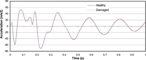
The time-dependent acceleration of a structure under a dynamical load contains proper information that can be used for damage identification. Any damage occurrence in the structure can be led to a change in structural acceleration. In order to investigate the sensitivity of acceleration responses as a time domain data to structural damage, a case study is made as follows. Consider the cantilevered beam shown in Figure 1 with a double damage cases modelled by a 20% reduction in modulus of elasticity of the 4th and 12th element of the beam. An impulse loading is applied at the end of the beam in y direction as shown in Figure 2 where F₀= 200 N and T₀= 0.15 s. Time history acceleration of 5th node is extracted in the healthy and damaged states and shown in Figure 3. As it is observed, the acceleration responses change due to the structural damage. Therefore, the time history acceleration responses are sensitive to structural damage and can be used as a damage indicator.

Figure 1. The cantilevered beam with a double damage cases under an impulse loading.

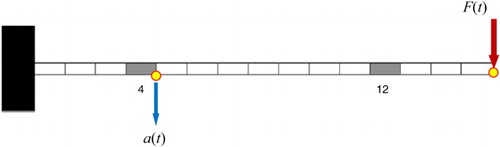
Figure 2. The impulse loading applied at the end node of the beam.

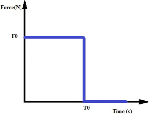
Figure 3. Time history acceleration response of 5th node in the healthy and damaged states.

3. The proposed damage detection method

The fundamental law for vibration-based damage detection methods is that damage alters mass, stiffness and damping characteristics of a structure. Such a change would lead to changes in the vibration properties of the structure, which is the key for identification of the damage by comparing the vibration responses of the structure before and after damage. The damage detection problem can be interpreted to find a set of damage variables minimizing/maximizing a correlation index between response data of a structure before and after damage [23–25]. Therefore, in this study, for finding the location and severity of damage in a structure, an optimization-based method is used as (8) $\begin{array}{ll}\text{Find:}& X^{\mathrm{T}}=\left\{x_1,x_2,\dots x_n\right\}\\ \text{Minimize:}& w\left(X\right)\\ & X^l\le X\le X^u\end{array}$(8) where $X^{\mathrm{T}}=\left\{x_1,x_2,\dots ,x_n\right\}$ is a damage variable vector containing the locations and sizes of n unknown damages; X^l and X^u are the lower and upper bounds of the damage vector. Also, w is an objective function that should be minimized.

3.1. Damage variables

The damage variable is defined here via a relative reduction of the elasticity modulus of a structural element as: (9) $x_i=\frac{E-E_i}{E}i=1,2,\dots ,n$(9) where E is the modulus of elasticity of healthy structure and E_i is the modulus of elasticity of the ith damaged element. In fact, in the equation, x_i is the ith component of the damage vector X, where x represents the severity of damaged element and i stands for the location of damaged element.

3.2. Objective function

Selecting the objective function for damage detection problems is a critical issue due to its fundamental role in the convergence of optimization algorithm. In many researches, various correlation indices have chosen as the objective function. In this study, an efficient objective function based on time-dependent accelerations in the limited points of the structure is defined as: (10) $w\left(X\right)=-\frac{{(a_d^{\mathrm{T}}.a(X\left)\right)}^2}{(a_d^{\mathrm{T}}.a_d)(a{\left(X\right)}^{\mathrm{T}}.a(X\left)\right)}$(10) where a_d is the acceleration response vector of damaged structure and a(X) is the acceleration response vector of an analytical model. The w varies from a minimum value −1 to a maximum value 0. It will be minimal when the vector of analytical acceleration response becomes identical to the acceleration response vector of the damaged structure, that is, a(X) = a_d.

For m number of measuring points (sensors), the acceleration response vectors (a_d and a(X)) would compile of m acceleration response vectors corresponding to m measuring point as defined in Equation (11). (11) $a_1=\left\{\right\},a_2=\left\{\right\},\dots a_m=\left\{\right\}\Rightarrow a=\left(\begin{array}{c}{a}_1\\ a_2\\ ⋮\\ a_m\end{array}\right)$(11) where a denotes the acceleration response vector used in the objective function, a₁, a₂ and a_m denote the acceleration response vectors corresponding to measuring points 1, 2 and m, respectively; and m denotes the number of measuring points (sensors).

3.3. The optimization algorithm

Since the optimization-based damage detection problem may have many local solutions, the selection of an efficient algorithm for solving the damage detection problem is of importance. In order to select a proper algorithm, achieving the global solution using fewer structural analyses is the main factor which must be considered. In this study, differential evolution algorithm (DEA) is employed to properly solve the problem.

In 1997, a new optimization algorithm called the DEA was proposed by Storn and Price [26]. The ability to finding the global solution and solving the nonlinear problems with a non-differentiable objective function is the main advantages of the algorithm. The main steps of the algorithm including Step 1: Initialization, Step 2: Mutation, Step 3: Crossover, Step 4: Selection and Step 5: Convergence can be explained as [26,27]:

Step 1: initialization

The initial parameters, constants and initial population are identified. Like other evolutionary algorithms, DEA starts to search from an initial population. The initial population is generated randomly in the search space as: (12) $X^l\le X_i\le X^u,i=1,2,\dots ,np$(12) where X^l and X^u are the lower and upper vectors of a variable vector, respectively. Also, np is the number of initial population that must be at least 4.

Step 2: mutation

For a given vector X_i (i = 1, 2, 3, … , np), a mutant vector is defined by a particular combination of three different current solutions as: (13) $V_i=X_{r_1}+mc.(X_{r_2}-X_{r_3}),r_{1\ne }{r}_{2\ne }{r}_{3\ne }i$(13) where the three different indices r₁, r₂ and r₃∈ {1, 2, 3, … , np} are randomly chosen to be different from index i. Also, mc ∈ [0, 2] is a real and constant factor which controls the amplification of the differential variation $(X_{r_2}-X_{r_3})$.

Step 3: crossover

In order to increase the diversity of the perturbed parameter vector, crossover is introduced by producing the trial vectors U_i (i = 1, 2, … , np) as: (14) $u_{ji}=\left\{\begin{array}{ll}{v}_{ji}& \text{if}\left(\text{ran}{\text{d}}_{ji}\le cc\text{or}j=\text{irn}{\text{d}}_i\right)\\ x_{ji}& \text{else}\end{array}\right.j=1,2,\dots ,n$(14) where rand_ji is a uniformly random number ∈ [0 1], cc is the crossover constant ∈ [0, 1] and irnd_i is a random integer ∈ {1, 2, … , n} which ensures that U_i gets at least one parameter from V_i.

Step 4: selection

For final selection, the target vector X_i is compared with the trial vector Ui. If the vector U_i yields a smaller objective function value than X_i, then X_i is set to U_i; otherwise, the old value X_i is retained.

Step 5: convergence

In this step, solution convergence is controlled. If the solution is converged, then the optimization is stopped; otherwise is returned to Step 2.

The flowchart of the proposed method can be briefly shown in Figure 4.

Figure 4. The flowchart of the proposed method.

4. Numerical examples and parametric study

In order to demonstrate the capabilities of the acceleration response based objective function (AROF) in combination with DEA for identification of the multiple-structural damage, three numerical examples, selected from the literature, are first considered and some parametric studies are conducted. The test examples are a 15-element beam, a 31-bar planar truss and 15-element planar frame are described below. At the end, a 45-element planar frame is considered for the assessment of the proposed method for a larger structure. The parameters of the DEA for all examples are also given in Table 1.

Table 1. The parameters of DEA for different examples.

Parameters	15-element beam	31-bar planar truss	15-element planar frame	45-element planar frame
np	60	75	45	60
mc	0.7	0.6	0.6	0.7
cc	0.3	0.3	0.1	0.1
kmax	3000	3000	2000	2000

Example 1: 15-element beam

A finite element model of a cantilevered beam [16] is constructed with 15 elements as shown in Figure 5. The numbers of elements and active nodes of the beam are displayed in the figure. The length, thickness and width of the beam are 2.74, 0.00635 and 0.0760 m, respectively. The mass density is 7860 kg/m³ and the elasticity modulus is 210 GPa. In this example, damage in the beam is simulated as a relative reduction in the elasticity modulus of individual elements. For constructing the objective function, an impulse loading of 200 N is applied to impact point of the beam shown in Figure 5. Five time history acceleration response vectors from the vertical direction of five measuring points of the beam are used for constructing the objective function. The total number of time steps is set to 1800 with an integration time step of 0.003 s, giving a total record time of 5.4 s. The parameters used for the DEA are given in Table 1. The convergence of the algorithm is met when the objective function reaches −1 or the maximum number of generations is attained.

Figure 5. 15-element beam with impact point.

Example 2: 31-bar planar truss

The 31-bar planar truss [16, 23] shown in Figure 6 is modelled using the conventional finite element method without internal nodes, leading to 25 active degrees of freedom as depicted in the figure. The numbers of elements and active nodes of the beam are displayed in the figure. The material density and elasticity modulus are 2770 kg/m³ and 70 GPa, respectively. Damage in the structure is also simulated as a relative reduction in the elasticity modulus of individual bars. An impact vertical force of 1000 N is applied at the impact point (node 13) and the accelerations of the truss are recorded at three measuring points as time history response. The total number of time steps is set to 300 with an integration time step of 0.01 s, giving a total record time of 3 s. All optimization parameters are listed in Table 1 and the convergence criteria are as the first example.

Figure 6. 31-bar planar truss with impact point.

Example 3: 15-element planar frame

A simple frame as shown in Figure 7 is considered as the third example. The numbers of elements along with the numbers of active nodes are depicted in the figure. The modulus of elasticity is 210 GPa and the material density is 7860 kg/m³. An impact horizontal force of 500 N is applied at the impact point as shown in Figure 7 and the horizontal accelerations of the frame are recorded at two measuring points as response time history data. The total number of time step is set to 400 with an integration time steps of 0.005 s, giving a total record time of 2 s. For this example, all the optimization parameters are summarized in Table 1 and the convergence criteria are similar to former examples.

Figure 7. 15-element planar frame with impact point.

4.1. Sensitivity study

4.1.1. Sensitivity to noise

In order to investigate the noise effects on the performance of the proposed method, a sensitivity study respect to measurement noise is considered here. For each example, as listed in Table 2, a damage scenario with two damaged elements is considered. Acceleration responses are extracted from measuring points given in Table 3 and contaminated with uniformly random noise with levels of 1%, 3% and 5% as: (15) $a_d^{\mathrm{noisy}}=a_d[1+(2\text{ random}-1\left)noise\right]$(15) where $a_d^{\mathrm{noisy}}$ and $a_d$ are the noisy damaged acceleration and damaged acceleration, respectively, noise is the level of noise considered and symbol random denotes a uniformly distributed random number on the interval [0 1].

Table 2. Damage scenarios for noise sensitivity study.

Example	Element number	Damage ratio
15-element beam	4	0.2
	12	0.2
31-bar planar truss	1	0.3
	2	0.2
15-element planar frame	5	0.2
	13	0.2

Table 3. Measuring points for noise sensitivity study

Example	Measuring points
15-element beam	1,4,7,10,13
31-bar planar truss	4(8^a), 7(12^a), 10(19^a)
15-element planar frame	3,12

^aDOF of truss

For the beam example, all acceleration data are extracted from vertical DOFs; for the frame, all the data are extracted from horizontal DOFs; and for the truss example, the accelerations are extracted from either of horizontal or vertical DOFs. The damage detection results of noise-free data along with noise contaminated data are shown in Figures 8–10 for beam, truss and frame, respectively. The results demonstrate the high efficiency of AROF in collaboration with DEA for determining the damage site and extent. The results presented in the figures express that the proposed method is capable of identifying the damage location and severity for various levels of noise. It is observed that the optimization process can obtain the actual site and extent of two damaged elements of the structures even in the high levels of noise.

Figure 8. Damage prediction of the beam for noise levels of (a) 0%, (b) 1%, (c) 3% and (d) 5%.

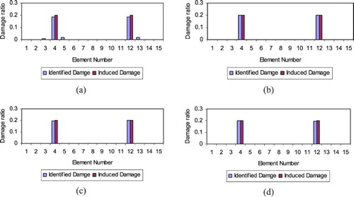
Figure 9. Damage prediction of the truss for noise levels of (a) 0%, (b) 1%, (c) 3% and (d) 5%.

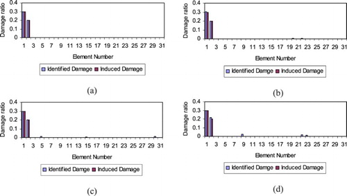
Figure 10. Damage prediction of the frame for noise levels of (a) 0%, (b) 1%, (c) 3% and (d) 5%.

4.1.2. Sensitivity to the number of damaged elements

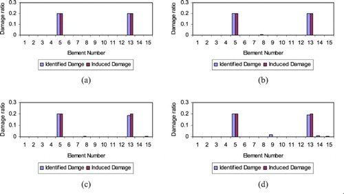
In order to investigate the capability of the proposed method to detect the damage of various elements, a sensitivity study is conducted. For this purpose, four damage scenarios are defined as listed in Table 4 with different numbers of damaged elements. Then acceleration responses are extracted from measuring points of each structure listed in Table 3 and contaminated with 3% noise. Then, the data are used for constructing the objective function. The predictions of the various damage scenarios using the proposed method are shown in Figures 11–13 for beam, truss and frame, respectively. It can be seen that for damage cases with various numbers and locations of damaged elements, the method can predict the damage elements with high accuracy.

Figure 11. Damage prediction of the beam for damage scenario (a) 1, (b) 2, (c) 3 and (d) 4.

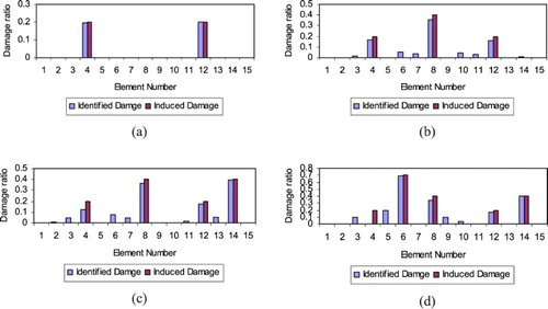
Figure 12. Damage prediction of the truss for damage scenario (a) 1, (b) 2, (c) 3 and (d) 4.

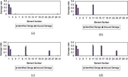
Figure 13. Damage prediction of the frame for damage scenario (a) 1, (b) 2, (c) 3 and (d) 4.

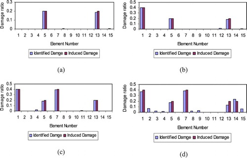
Table 4. Damage scenarios for damage case sensitivity study.

	Example
Damage scenario	15-element beam	31-bar planar truss	15-element planar frame
1	4(0.2)^a–12(0.2)	1(0.3)–2(0.2)	5(0.2)–13(0.2)
2	4(0.2)–8(0.4)–12(0.2)	1(0.3)–2(0.2)–11(0.25)	1(0.4)–5(0.2)–13(0.2)
3	4(0.2)–8(0.4)–12(0.2)–14(0.4)	1(0.3)–2(0.2)–	1(0.4)–5(0.2)–
		11(0.25)–25(0.15)	7(0.4)–13(0.2)
4	4(0.2)–6(0.7)-8(0.4)–12(0.2)–14(0.4)	1(0.3)–2(0.2)–11(0.25)–	1(0.4)–5(0.2)–7(0.4)–
		16(0.3)–25(0.15)	13(0.2)–14(0.2)

^aThey represent damaged element (damage ratio).

4.1.3. Sensitivity to measuring points

Since the acceleration responses are extracted from a limited number of measuring points, the selection of proper sensor places, including the most informative data, is of importance. In order to investigate the effects of the sensor places on the accuracy of damage detection method, four random sensor networks are considered and a sensitivity study is conducted. For this purpose, for each structure, the damage scenario with two damaged elements given in Table 2 is considered. Then, four different sets of sensor networks are defined as given in Table 5 and acceleration response vectors are extracted from these points. The time history response data are contaminated with 3% noise and used for constructing the objective function. The damage detection results are shown in Figures 14–16. As shown in the figures, for all the networks, the proposed method can predict the damage extent and location with high accuracy, which means that the damage prediction outcomes are independent from the measuring points.

Figure 14. Damage prediction of the beam for sensor network (a) 1, (b) 2, (c) 3 and (d) 4.

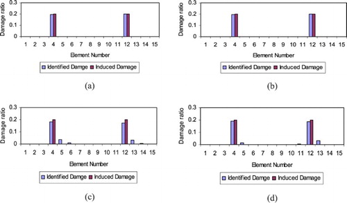
Figure 15. Damage prediction of the truss for sensor network (a) 1, (b) 2, (c) 3 and (d) 4.

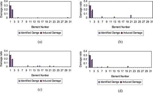
Figure 16. Damage prediction of the frame for sensor network (a) 1, (b) 2, (c) 3 and (d) 4.

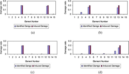
Table 5. Sensor networks for measuring point sensitivity study.

	Measuring points
Example	Sensor network 1	Sensor network 2	Sensor network 3	Sensor network 4
15-element beam	1,4,7,10,13	1,5,7,9,14	2,3,7,13,14	3,5,7,9,11
31-bar planar truss	4(8)^a,7(12),10(19)	1(2),6(11),12(22)	2(4),5(10),7(13)	3(6),7(13),11(20)
15-element planar frame	3, 12	2, 3	6, 8	12, 13

^aThey represent node number (DOF) of the truss for measuring acceleration.

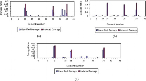
4.2. 45-element frame

The 45-element frame [28] shown in Figure 17 is considered to assess the performance of the proposed method when a larger structure and a high level of noise are investigated. The numbers of elements and nodes are shown in the figure. The Young’s modulus and the material density are 210 GPa and 7780 kg/m³, respectively. The section used for the columns is (W14×145) and for the beams is (W12×87). An impact horizontal force of 1000 N is applied at node 6 and the horizontal accelerations of the frame are recorded at three measuring points (nodes 4, 10, 11) as response time history data. The integration time step is set to 0.03 s and the total record time is 3 s. All optimization parameters are summarized in Table 1 and the convergence criteria are similar to the first example. Three damage scenarios are considered as given in Table 6.

Figure. 17. 45-element frame subjected to an impact point.

Table 6. Damage scenarios for the frame.

Scenario 1		Scenario 2		Scenario 3
Element	Damage ratio	Element	Damage ratio	Element	Damage ratio
10	0.25	14	0.35	9	0.30
30	0.20	28	0.30	18	0.20
40	0.25	38	0.35	36	0.25

The performance of the method without considering noise and with contaminating 10% and 15% noise are displayed in Figures 18–20, respectively. Results show that the proposed method can properly identify when noise is ignored; also it is observed that the outcomes considering 10% noise possess adequate precision. Even though, considering the 15% noise makes some disorders to find damage in case 1, however, damage cases 2 and 3 are appropriately identified.

Figure 18. Damage prediction of the frame without considering noise for (a) Scenario 1, (b) Scenario 2 and (c) Scenario 3.

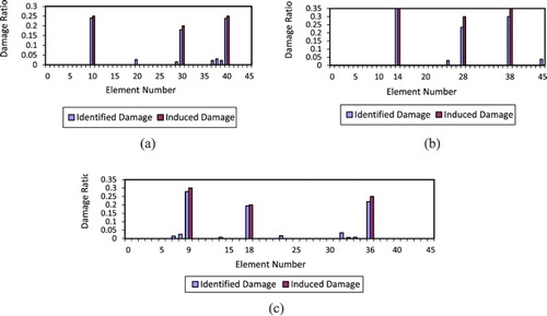
Figure 19. Damage prediction of the frame contaminating 10% noise for (a) Scenario 1, (b) Scenario 2 and (c) Scenario 3.

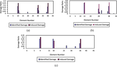
Figure 20. Damage prediction of the frame contaminating 15% noise for (a) Scenario 1, (b) Scenario 2 and (c) Scenario 3.

5. Conclusion

This paper presents a thorough investigation of a vibration-based damage detection technique, which utilizes an efficient optimization algorithm in combination with acceleration responses-based objective function, to identify the location and severity of multiple damages in structures. Firstly, the damage detection problem is formulated as a standard optimization problem aiming to minimize an objective function for finding continuous damage variables. The objective function has been defined based on a vector containing acceleration responses extracted from a limited number of measuring points. The DEA as a global optimization algorithm is utilized to properly solve the optimization problem. In order to assess the competence of the proposed approach for structural damage detection, four illustrative examples are numerically tested. Up to 15% noise is added to numerical data to consider uncertainty, and a noise sensitivity study is conducted to investigate the noise robustness of the developed method. Numerical results considering the measurement noise demonstrate that the combination of AROF and DEA can provide a robust tool for structural damage detection, even in high noise levels (15%). The results of parametric studies show that the damage identification scheme developed is robust with respect to measuring points. In other words, the influence of sensor places to the damage prediction outcomes is negligible in small structures. In addition, the method is capable of identifying various numbers and places of damaged elements. The proposed method has the capability to cope with incomplete vibration data obtained from a limited number of measuring points. In comparison with modal based methodologies, the method requires much less post-processing on the recorded data and fewer measuring points; which makes the proposed method more suitable for online health monitoring.

Disclosure statement

No potential conflict of interest was reported by the authors.

References

- Lifshitz JM, Rotem A. Determination of reinforcement unbonding of composites by a vibration technique. J Compos Mater. 1969;3(3):412–423. doi: 10.1177/002199836900300305
- Adams RD, Cawley P, Pye CJ, et al. A vibration technique for non-destructively assessing the integrity of structures. J Mech Eng Sci. 1978;20(2):93–100. doi: 10.1243/JMES_JOUR_1978_020_016_02
- Maity D, Tripathy RR. Damage assessment of structures from changes in natural frequencies using genetic algorithm. Struct Eng Mech. 2005;19(1):21–42. doi: 10.12989/sem.2005.19.1.021
- Pawar PM, Ganguli R. Matrix crack detection in thin-walled composite beam using genetic fuzzy system. J Intell Mater Syst Struct. 2005;16(5):395–409. doi: 10.1177/1045389X05051001
- Chen HL, Spyrakos CC, Venkatesh G. Evaluating structural deterioration by dynamic response. J Struct Eng. 1995;121(8):1197–1204. doi: 10.1061/(ASCE)0733-9445(1995)121:8(1197)
- Trendafilova I. A study on vibration-based damage detection and location in an aircraft wing scaled model. Appl Mech Mater. 2006;3(4):309–314. doi: 10.4028/www.scientific.net/AMM.3-4.309
- Kim JT, Park JH, Lee BJ. Vibration-based damage monitoring in model plate-girder bridges under uncertain temperature conditions. Eng Struct. 2007;29(7):1354–1365. doi: 10.1016/j.engstruct.2006.07.024
- Shi ZY, Law SS, Zhang LM. Damage localization by directly using incomplete mode shapes. J Eng Mech. 2000;126(6):656–660. doi: 10.1061/(ASCE)0733-9399(2000)126:6(656)
- Parloo E, Guillaume P, Van Overmeire M. Damage assessment using mode shape sensitivities. Mech Syst Signal Process. 2003;17(3):499–518. doi: 10.1006/mssp.2001.1429
- Elshafey AA, Marzouk H, Haddara MR. Experimental damage identification using modified mode shape difference. J Mar Sci Appl. 2011;10(2):150–155. doi: 10.1007/s11804-011-1054-5
- Huth O, Feltrin G, Maeck J, et al. Damage identification using modal data: experiences on a prestressed concrete bridge. J Struct Eng. 2005;131(12):1898–1910. doi: 10.1061/(ASCE)0733-9445(2005)131:12(1898)
- Alvandi A, Cremona C. Assessment of vibration-based damage identification techniques. J Sound Vib. 2006;292(1–2):179–202. doi: 10.1016/j.jsv.2005.07.036
- Lu XB., Liu, JK., Lu, Z.R. A two-step approach for crack identification in beam. J Sound Vib 2013; 332(2):282–293. doi: 10.1016/j.jsv.2012.08.025
- Dawari VB, Vesmawala GR. Modal curvature and modal flexibility methods for honeycomb damage identification in reinforced concrete beams. Procedia Eng. 2013;51:119–124. doi: 10.1016/j.proeng.2013.01.018
- Choi S, Park S, Yoon S, et al. Nondestructive damage identification in plate structures using changes in modal compliance. NDT E Int. 2005;38(7):529–540. doi: 10.1016/j.ndteint.2005.01.007
- Seyedpoor SM. A two stage method for structural damage detection using a modal strain energy based index and particle swarm optimization. Int J Non Linear Mech. 2012;47(1):1–8. doi: 10.1016/j.ijnonlinmec.2011.07.011
- Fang X, Tang J. Frequency response based damage detection using principal component analysis. Proceedings of IEEE International Conference on Information Acquisition, Hong Kong and Macau, China, 2005; 407–412.
- Bandara RP, Chan THT, Thambiratnam DP. Structural damage detection method using frequency response functions. Struct Health Monit. 2014;13(4):418–429. doi: 10.1177/1475921714522847
- Zimin V, Zimmerman DC. Structural damage detection using time domain periodogram analysis. Struct Health Monit. 2009;8(2):125–135. doi: 10.1177/1475921708094796
- Fu YZ, Lu ZR, Liu JK. Damage identification in plates using finite element model updating in time domain. J Sound Vib. 2013;332(26):7018–7032. doi: 10.1016/j.jsv.2013.08.028
- Bagheri A, Kourehli S. Damage detection of structures under earthquake excitation using discrete wavelet analysis. Asian J Civ Eng. 2013;14(2):289–304.
- ANSYS, Inc. Theory Reference (2006) Release 10.0 Documentation for ANSYS, ANSYS Inc.; 2006.
- Nobahari M, Seyedpoor SM. Structural damage detection using an efficient correlation based index and a modified genetic algorithm. Math Comput Model. 2011;53(9–10):1798–1809. doi: 10.1016/j.mcm.2010.12.058
- Seyedpoor SM. Structural damage detection using a multi-stage particle swarm optimization. Adv Struct Eng. 2011;14(3):533–549. doi: 10.1260/1369-4332.14.3.533
- Kourehli SS, Bagheri A, Ghodrati Amiri G, et al. Structural damage identification based on incomplete static responses as an optimization problem. Scientia Iranica. 2014;21(4):1209–1216.
- Storn R, Price K. Differential evolution–a simple and efficient heuristic for global optimization over continuous spaces. J Glob Optim. 1997;11(4):341–359. doi: 10.1023/A:1008202821328
- Shahbandeh S, Seyedpoor SM, Yazdanpanah O. An efficient method for structural damage detection using a differential evolution algorithm based optimization approach. Civ Eng Environ Syst. 2015;32(3):230–250. doi: 10.1080/10286608.2015.1046051
- Kaveh A, Javadi SM, Maniat M. Damage assessment via modal data with a mixed particle swarm strategy, ray optimizer and harmony search. Asian J Civ Eng. 2014;15(1):95–106.