Inverse estimation of variable thermal parameters in a functionally graded annular fin using dragon fly optimization

ABSTRACT

This paper presents an inverse study of heat transfer of a conductive, convective and radiative annular fin made of a functionally graded material. Three major parameters such as conductive–convective parameter, conductive–radiative parameter and the parameter describing the variation of thermal conductivity are inversely estimated from a specified temperature field. The forward solution of temperature field is obtained from the closed form solution of nonlinear heat transfer equation using Homotopy perturbation method (HPM). A dragonfly algorithm that simulates the swarming behaviour of dragonflies, as analogous, is employed in finding out the inverse parameters. The temperature values of the forward solution are used as input data for the inverse analysis. The inverse parameters are then estimated iteratively by minimizing the objective function until the guessed temperature field approximately satisfies the preassigned temperature field of the forward solution. The inverse simulation following HPM-based forward solution converges faster than ordinary differential equation-based forward solution. The reconstructed temperature fields obtained from the various combination of inverse parameters give good agreement (∼1% error) with the desired temperature field. Thus, the presented inverse model provides an opportunity to the fin designer for selecting the several feasible combinations of thermal parameters suggesting the material design that result in a prescribed temperature field.

KEYWORDS:

• Inverse study
• functionally graded fin
• nonlinear heat transfer
• variable parameters

AMS/MSC SUBJECT CLASSIFICATIONS:

• 80A23
• 31B20
• 80A20
• 80M50

1. Introduction

Fins are extended surfaces used to transfer excess heat from a primary surface, such as on the equipment, to the surroundings for maintaining the operating temperature at the primary surface [1]. Fins enhance the heat transfer rate by providing an increased surface area to the adjacent coolant. They are used as cooling agents in a variety of equipment including internal combustion engines, compressors, heat exchangers, transformers, nuclear rods, space radiators, electronic devices. Among the various types of fins, annular fins are more popular and of current research interest because of their compact design. An annular fin provides more surface area in contact with the coolant as compared to a straight fin of comparable dimension. Due to the compact design and ease of manufacturing, annular fin with constant thickness is most favourable for use in tube heat exchangers.

Due to the increasing demand of fins with lighter weight, faster heat transfer rate, and better structural stability, modern materials are more attractive nowadays in comparison to conventional materials. However, most of the fin studies assume conventional material due to the mathematical complexity in the analysis and limitation of the manufacturing process associated with the modern materials. In the recent past, few researchers had studied the heat transfer of fins made of functionally graded materials (FGMs). Most of these studies addressed only conductive–convective fin where the conductive parameter was considered to a function of the length of the fin [2,3]. However, the fact is that other thermal parameters have a significant effect too and cannot be ignored. The rectangular fin with temperature dependent power-law variation of thermal conductivity and emissivity were studied by Campo and Wolko [4]. Lesnic and Heggs [5] employed decomposition method to study the temperature distribution in a straight fin with a power variation of temperature dependent heat transfer coefficient.

Khan and Aziz [6] studied the numerical analysis of transient and steady-state heat transfer analysis of a functionally graded convecting longitudinal fin. Further, Aziz et al. [7] proposed differential transformation method for the analysis of homogeneous and FGM convective–radiative radial fin with convective base heating and convective–radiative tip cooling. Hassanzadeh and Pekel [8] employed mean value theorem for studying local temperature field and heat transfer rate in an FGM annular fin. The result showed that a fin made of FGM enhances the heat transfer rate as compared with a homogeneous one. The study of FGM fin with the variability of all parameters of heat transfer, including conduction, convection, radiation and heat generation, requires solving fourth-order nonlinear equation of heat transfer with multiple nonlinearities. A comprehensive literature search reveals that study of the heat transfer in an FGM fin considering large numbers of variable parameters has not been reported so far. Peng and Li [9] reported that the general form of the variation of material properties in FGM follows the power law with special coordinates. The variation of thermal parameters significantly influence the local temperature distribution, and hence the performance of fin. Thus, estimation of the various thermal parameters should be of high priority in FGM fin design. Although some basic studies of FGM fin were reported by few researchers, inverse analysis for the same is still lacking. The forward analysis by solving the heat transfer equation is well posed. In this case, the results are obtained using the known thermal parameters. However, the problem becomes more complicated and challenging if the final objective of the problem (i.e. thermal distribution) is known and the thermal parameters satisfying the objective are unknown. Such inverse problem is mathematically ill-posed and thus difficult to solve.

Inverse problems of heat transfer are gaining significant attention in the field of science and engineering due to time-saving production of low-cost equipment with desired outputs. It has wide applications in several fields [10–13]. The average heat transfer coefficient was estimated by Chen and Hsu [14] using the finite difference method coupled with least-squares method. Słota [15] applied genetic algorithms to determine the heat transfer coefficient in three-phase inverse Stefan problem and reported that the result obtained was more accurate than the Nelder–Mead’s method. Inverse heat conduction problem was presented by Hetmaniok et al. [16] using homotopy perturbation method (HPM). Yu et al. [17] developed a meshless inverse method to estimate the temperature field and heat flux distribution in a 2D steady-state heat conduction problem. A hybrid optimization technique coupled with the scaled boundary finite element method was employed by Mohasseba et al. [18] for investigating the unknown heat flux in a transient heat conduction problem. An inverse solution for two-dimensional hyperbolic heat conduction problem was realized by finite difference method using modified Newton–Raphson method [19]. The correctness of the method was asserted by comparing the results with an analytical solution of the problem. A wide verity of inverse study based on numerical approach on the heat transfer problem is available in the book of Ozisik and Orlande [20]. Lesnic and Elliott [21] employed the Adomian’s decomposition method for an inverse study of boundary value problem in heat conduction. In their analysis, the stable approximate solution was obtained by controlling noisy input data using mollification method. Genetic algorithm-based multi-objective optimization was applied by Hajabdollahi [22] for determining optimal geometry of pin fin, respectively. Bamdad and Ashorynejad [23] estimated base temperature and heat flux in rectangular fin by combining adjoint conjugate gradient method and lattice Boltzmann method. Simulated annealing was employed by Chang et al. [24] for solving optimal chiller loading problem. Das et al. [25] employed simplex search method to predict the thermal parameters. Attention has not yet been paid towards the inverse estimation of thermal parameters for an FGM fin. Only Lee et al. [26] applied an inverse algorithm based on conjugate gradient method to study the time-dependent base heat flux and temperature distributions of a functionally graded radial fin.

The main objective of the present work is to estimate the three major unknown thermal parameters of a functionally graded annular fin. By proper tuning these parameters, one can obtain the desired heat transfer and efficiency without compromising the volume of the fin. The recently proposed dragonfly algorithm (DA) [27], based on the swarming behaviour of dragonflies, has been employed for this purpose.

2. Problem formulation

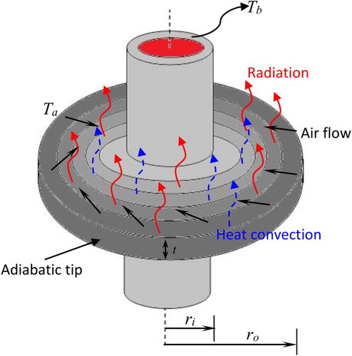
The analysis of a fin is considered the problem to maximize the heat transfer from the hot body, preferably from the fin’s surface to the surrounding. The annular fin, made of FGM, with inner radius, r_i, outer radius, r_o, and thickness t as shown in Figure 1 is considered. The fin is subjected to a base temperature T_b, and its tip is assumed to be well insulated. The heat loss from the surface takes place by convection and radiation simultaneously. The ambient and surrounding temperatures of convection and radiation are taken as T_a and T_s, respectively. The thermal conductivity, k, of the fin material is linearly proportional to the spatial co-ordinate r and the emissivity ε is considered to be varying nonlinearly with r. A similar interpretation is made for internal heat generation q and convective heat transfer coefficient h which vary with temperature T only.

Figure 1. Geometry of an annular fin made of FGM.

3. Governing equation

3.1 Heat transfer equation

Fourier’s law of heat conduction is applicable to the present problem. Considering the fin with a negligible heat loss at the base and the tip is well insulated (i.e. adiabatic tip), the steady-state energy balance equation and its associated boundary conditions can be expressed as [1], (1) $t\frac{\text{d}}{\text{d}r}\left[\left\{k\left(r\right)\right\}r.\frac{\text{d}T}{\text{d}r}\right]-2h\left(T\right)r(T-T_a)-2\epsilon \left(r\right)\sigma r(T^4-T_s^4)+q\left(T\right)\text{tr}=0,$(1) $T=T_b$ at $r=r_i$ and $\frac{\text{d}T}{\text{d}r}=0$ at $r=r_{\mathrm{o}}$.

The following mathematical relations hold for the variation of the associated thermal parameters: (2) $\begin{array}{rl}& k=k_{\mathrm{o}}\left\{1+\gamma \left(\frac{r-r_i}{r_o-r_i}\right)\right\},h=h_{\mathrm{b}}{\left(\frac{T-T_{\mathrm{a}}}{T_{\mathrm{b}}-T_{\mathrm{a}}}\right)}^{m_1},\epsilon ={\epsilon }_{\mathrm{s}}{\left(\frac{r}{r_i}\right)}^{m_2}\text{and}\\ & q=q_{\mathrm{o}}\left\{1+e\left(T-T_{\mathrm{a}}\right)\right\},\end{array}$(2) where, k_o is the thermal conductivity at the base of the fin, h_b is the convective heat transfer coefficient to the temperature difference T_b−T_a, ε_s is the surface emissivity at the base of the fin and q_o is the internal heat generation at ambient temperature T_a. The parameter γ is an inhomogeneity index describing the variation of thermal conductivity of the FGMs which play an important role on the thermal behaviour of the fin. The constant, e represents the variation of internal heat generation, respectively. The parameters, m₁ and m₂ are the power law index for the variation of convective and radiative heat transfer coefficient. The index m₁ indicates the heat transfer mode [5]. The radius of the fin, at any point is given as r, and σ is the Stefan–Boltzmann constant. The following non-dimensional terms are introduced for simplicity and wider application: (3) $\begin{array}{rl}\theta & =\frac{T}{T_{\mathrm{b}}},{\theta }_{\mathrm{a}}=\frac{T_{\mathrm{a}}}{T_{\mathrm{b}}},{\theta }_{\mathrm{s}}=\frac{T_{\mathrm{s}}}{T_{\mathrm{b}}},\xi =\frac{r-r_i}{r_i},R=\frac{r_{\mathrm{o}}}{r_i},N_{\mathrm{c}}^2=\frac{2h_{\mathrm{b}}{r_i}^2}{k_{\mathrm{o}}t},\delta =\frac{t}{r_i},\\ N_{\mathrm{r}}& =\frac{2\sigma {\epsilon }_{\mathrm{s}}{r}_i^2{T}_{\mathrm{b}}^3}{k_{\mathrm{o}}t},G=\frac{q_{\mathrm{o}}{r}_i^2}{k_{\mathrm{o}}{T}_{\mathrm{b}}},\text{and}{E}_{\mathrm{G}}=e{T}_{\mathrm{b}},\end{array}$(3) where θ is the non-dimensional temperature field varying with non-dimensional radius ξ. The parameters, θ_a representing non-dimensional convective environment temperature, θ_s representing non-dimensional surrounding temperature for radiation, R is the annular ratio, N_c is the alternate convection–conduction number, N_r is the alternate radiation–conduction number, δ is the thickness ratio, G is the heat generation number and E_G is non-dimensional parameter describing the variation of heat generation. After substituting the above non-dimensional terms, the energy balance equation and the corresponding boundary conditions can be expressed in the following dimensionless form: (4a) $\begin{array}{rl}& \frac{d^2\theta }{\text{d}{\xi }^2}+\frac{\gamma \xi }{\left(R-1\right)}\frac{d^2\theta }{\text{d}{\xi }^2}+\frac{\gamma }{\left(R-1\right)}\frac{\text{d}\theta }{\text{d}\xi }+\frac{1}{\left(1+\xi \right)}\frac{\text{d}\theta }{\text{d}\xi }+\frac{\gamma }{\left(R-1\right)}\frac{\xi }{1+\xi }\frac{\text{d}\theta }{\text{d}\xi }\\ & -N_{\mathrm{c}}^2\frac{{\left(\theta -{\theta }_{\mathrm{a}}\right)}^{\left(m_1+1\right)}}{{\left(1-{\theta }_{\mathrm{a}}\right)}^{m_1}}\\ & -N_{\mathrm{r}}(1+\xi {)}^{m_2}\left({\theta }^4-{\theta }_{\mathrm{s}}^4\right)+G\left\{1+E_{\mathrm{G}}\left(\theta -{\theta }_{\mathrm{a}}\right)\right\}=0\end{array}$(4a) (4b) $\theta =1\text{at}\xi =0\text{and}\frac{\text{d}\theta }{\text{d}\xi }=0\text{at}\xi =R-1.$(4b)

3.2. HPM solution for temperature distribution

Here, we introduce the concept of the HPM solution. He’s formulation is restated for a general nonlinear differential equation as follows [28,29]: (5a) $L\left(\theta \right)-NL\left(\theta \right)-f\left(r\right)=0,r\in \mathrm{\Omega }$(5a) with the corresponding boundary conditions, (5b) $B\left(\theta ,\frac{\mathrm{\partial }\theta }{\mathrm{\partial }n}\right)=0,r\in \mathrm{\Gamma }$(5b) The terms, L and N are the linear and nonlinear operator, f(r) is a known an analytical function, B is the boundary operator, and Γ is the boundary of the domain Ω.

Now, constructing homotopy for a given nonlinear differential equation as, (6) $(1-p)\left[L\right(\theta )-L({\theta }_{\mathrm{o}}\left)\right]+p\left[L\right(\theta )+NL(\theta )-f(r\left)\right]=0,$(6) where, $L=\frac{d^2}{\text{d}{\xi }^2},$ p∈[0, 1] is an embedding parameter which changes monotonically from 0 to 1. According to HPM, the embedding parameter p can initially be used as a small parameter and the solution of Equation (6) can be represented in the form of power series in p. The details about the embedding parameter, p, is available in the articles of He [28], Shakeri and Dehghan [30] and Mallick et al. [31]. After applying HPM, the energy balance equation can be rewritten in the following form: (7) $\begin{array}{rl}& -L\left({\theta }_0\right)+L\left({\theta }_0+p{\theta }_1+p^2{\theta }_2\right)+pL\left({\theta }_0\right)+p\left[\frac{\gamma \xi }{\left(R-1\right)}\ddot{\theta }+\frac{\gamma }{\left(R-1\right)}\dot{\theta }+\frac{1}{\left(1+\xi \right)}\dot{\theta }+\right.\\ & \left.\frac{\gamma }{\left(R-1\right)}\frac{\xi }{1+\xi }\dot{\theta }-N_{\mathrm{c}}^2\frac{{\left(\theta -{\theta }_{\mathrm{a}}\right)}^{\left(m_1+1\right)}}{{\left(1-{\theta }_{\mathrm{a}}\right)}^{m_1}}-N_{\mathrm{r}}{\left(1+\xi \right)}^{m_2}\left({\theta }^4-{\theta }_{\mathrm{s}}^4\right)+G\left\{1+E_{\mathrm{G}}\left(\theta -{\theta }_{\mathrm{a}}\right)\right\}\right]=0.\end{array}$(7)

The solution for the non-dimensional temperature field is obtained by considering p = 1 and seperating the variables of identical powers as, (8) $\theta \left(\xi \right)={\theta }_0\left(\xi \right)+p{\theta }_1\left(\xi \right)+p^2{\theta }_2\left(\xi \right)+\dots ,$(8)

The details pertaining to the solution and boundary conditions are presented in our published articles [31,32].

4. Inverse design for fin parameters

The inverse problem is inferring the cause from a known effect. For heat transfer problems of fins, it usually implies finding the thermal parameters of a fin for a given temperature field. The inverse problem, in general, is ill-posed. It becomes even more complicated if the underlying forward model is nonlinear, i.e. the temperature on the fin is a nonlinear function of the unknown parameter. In order to make an efficient design of fin, the various parameters that involved in heat transfer are to be estimated properly. To innovate the best possible design solution, these parameters are to be predicted in such a way that the cost of the fin is small and good efficiency is obtainable. Thus, the inverse estimation of the fin parameters is very important for the smart design of heat transfer equipment. In this analysis, the three non-dimensional thermal parameters, such as, thermo-geometry parameter (N_c), conduction-radiation parameter (N_r) and variable thermal conductivity parameter (γ) are considered to be inverse parameters. These three parameters affect the heat transfer, and thus, the temperature distribution along the fin length. For a predefined temperature field, these parameters can be optimized using the retrieval methodology. In order to solve the inverse problem, the following objective function is to be minimized: (9) $\mathrm{\Re }\left(\xi \right)=\sqrt{\sum _{i=1}^P\left[{\left({\theta }_i\left(\xi \right)-{\theta }_i^{\ast }\left(\xi \right)\right)}^2/P\right]},$(9) where, P is the total number of locations where the objective function value is to evaluate. Various nature-inspired optimization techniques have been developed in last few decades for the inverse analysis. Among them, we use the recently proposed DA for the inverse parametric study of FGM annular fin.

4.1 Dragon fly algorithm

The DA developed by Mirjalili [27] is inspired by and related to the particle swarm optimization (PSO). It selects a set of random solutions as an analogue of a population of dragonflies. The initial swarm is selected randomly from the solution space. The ability of stochastic population-based optimization approaches of PSO algorithms, including the DA, is a central strength of these algorithms. It makes these algorithms less sensitive to the unavailability of suitable initial guess. Furthermore, it allows the exploration of multiple solutions in the solution space which might not be possible if an initial guess is provided which dominates the progress of algorithm towards the local minimum close to the initial guess. The solution space is defined by the upper bound and lower bound for each unknown parameter. The cost function is computed for each dragonfly in the population. In each iteration, the swarm of dragonflies moves towards finding sources of food, which is analogous to the local minima of the cost function and moving away from predators or enemies, which is analogous to local maxima of the cost function. The largest source of food corresponds to the global minimum. The swarm’s behaviour maintains the following rules:

1. Avoid crowding to minimize the collision of individual dragonflies from the neighbouring dragonflies. This is referred to as maintaining separation.

2. Match the velocity of the neighbouring dragonflies. This is referred to as maintaining or improving alignment.

3. To make an interconnection, move towards the centre of mass of all dragonflies. This is referred to as improving cohesion.

If the current position of the ith individual is represented by X_i and its jth neighbouring individuals are X_ji, j = 1 to N, then the separation of ith individual (S_i) is estimated as, (10) $S_i=-\sum _{j=1}^N\left[X_i-X_{ji}\right],$(10) where, N is the number of neighbouring individuals. If V_ji is the velocity of jth individuals in the neighbourhood of X_i, then the alignment of ith individual (A_i) is calculated as, (11) $A_i=\frac{{\sum }_{j=1}^N{V}_{ji}}{N}.$(11)

The cohesion of ith individual (C_i) is calculated as, (12) $C_i=\frac{{\sum }_{j=1}^N{X}_{ji}}{N}-X_i.$(12)

The attraction towards the food of ith individual (F) source and the distraction of ith individual from the enemy are mathematically represented as, (13) $F_i={X_i}^{+}-X_i\text{ and }{E}_i={X_i}^{-}+X_i,$(13) where, $X_i^{+}$ and $X_i^{-}$ are the position of the food source and the position of the enemy from the current position of the ith individual. The behaviour of every individual depends on the above five parameters (i.e. S_i, A_i, C_i, F_i, and E_i,). Optimization to the global minimum can be achieved by tweaking the current position and velocity of each individual in proportion to these parameters. During the optimization process, the movements of the dragonflies are updated by introducing a step vector, ΔX, through the following equation: (14) $\mathrm{\Delta }{X}_{t+1}=\left(s{S}_i+a{A}_i+c{C}_i+f{F}_i+e{E}_i\right)+w\mathrm{\Delta }{X}_t,$(14) where, s, a, c, f and e are the factors of separation, attraction, cohesion, food, and enemy, respectively. These parameters are updated in the algorithm on the fly, depending upon the progress of the dragonfly population. The initial values are assigned randomly. The term w represents the inertia weight, and t is the iteration counter. The inertia weight is assigned a value 0.9 in the beginning and its value evolves with the iterations. The details of the update mechanisms can be found in [27]. Once the step vector is estimated, the position vector is updated as, (15) $\mathrm{\Delta }{X}_{t+1}=X_t+\mathrm{\Delta }{X}_{t+1}.$(15)

As iterations progress, the value of $\mathrm{\Delta }{X}_{t+1}$ may become small and the swarm may become static, which is a consequence of reaching a minimum (i.e. a local source of food). This is referred to as the exploitation state as opposed to exploratory state when $\mathrm{\Delta }{X}_{t+1}$ is large. In nonlinear problems, such as the heat transfer problem of FGM annular fin, the swarm may be exploiting a local source of food (a local minimum) instead of the largest source of the food (the global minimum). Thus, three mechanisms for transition from the exploitation phase to the exploratory phase are incorporated. The first mechanism is to increase the radius of neighbourhood linearly with the iteration number. The second mechanism is to adaptively tune the factors s, a, c, f and e in order to balance exploitation and exploration. The third mechanism is to incorporate random flight when there is no dragonfly in neighbourhood of a dragonfly through the following formula for updating its: (16) $\mathrm{\Delta }{X}_{t+1}=X_t+\text{L'{e}vy(d )}\times X_t,$(16) where, d is the dimension of position vectors and t is the current iteration. The Lévy flight is represented by, (17) $\text{L'{e}vy}\left(d\right)=0.01\times \frac{r_1\times \tilde{\sigma }}{{|r_2|}^{1/\beta }},$(17) where, r₁ and r₂ represent random numbers in [0,1] and β is a constant. The parameter, $\tilde{\sigma }$ is given by (18) $\tilde{\sigma }={\left(\frac{\mathrm{\Gamma }\left(1+\beta \right)\times \sin \left(\frac{\pi \beta }{2}\right)}{\mathrm{\Gamma }\left(\frac{1+\beta }{2}\right)\times \beta \times 2^{\left(\frac{\beta -1}{2}\right)}}\right)}^{1/\beta }\text{with }\mathrm{\Gamma }\left(x\right)=(x-1)!$(18)

In this algorithm, the step vectors and positions are initially guessed in between lower bound and upper bound variables. We note that Γ(x) is the well-known gamma function. Through Equations (14)–(16), the values of the variables are updated in every iteration. The updating process of the variables is continued until the cost function is minimized or the difference between the cost functions in successive iterations becomes negligible.

5. Results and discussion

The focus of this study is inverse estimation of unknown thermal parameters, N_c, N_r and γ, satisfying a prescribed/given temperature field in an FGM annular fin. It is well known that the thermal performance of an annular fin depends on the various thermal parameters. Therefore, the optimization of the various thermal parameters is an utmost necessity for an efficient and cost-effective fin design. The prescribed temperature field may be a design requirement. For the inverse estimation of thermal parameters, DA algorithm was employed which requires computation of the temperature field corresponding to each individual in the swarm in each iteration. HPM forward solution is being used for this purpose as well.

Prior to using the closed form solution in the inverse study, the HPM-based results were validated with the results reported in the literature and the results obtained using finite element method (FEM) and numerical solution for the ordinary differential equation (ODE) given in Equation (4) using Runge–Kutta method. The FEM solution is obtained using COMSOL Multiphysics [33] software. Matlab’s in-built ODE solver is used for Runge–Kutta method [34]. Due to the limitation of available literature results, the present HPM solution is validated with Chiu and Chen’s result for isotropic material [35]. The comparison is given in Table 1. In order to the completeness of the HPM-based forward solution of FGM model, the results are also compared with FEM and ODE as well in Table 1. The results are presented in both dimensional and non-dimensional form. In the non-dimensional analysis, it can be seen that the HPM result deviates 2.08% from Chui-Chen and 0.098% from the ODE results. The higher deviation from Chui-Chen’s result is due to consideration of absorptivity (α) parameter in their analysis. On the other side, the HPM solution for FGM fin (considering all non-zero parameters) show only 0.0747% and 0.4302% deviation in comparison with ODE and FEM results, respectively. Thus, the present HPM-based closed form solution is in good agreement with the available literature results as well as the results of the numerical solution of FGM annular fin. Moreover, the results suggest that the present HPM model is equally suitable for dimensional and non-dimensional analysis. We note that the various non-dimensional parameters, N_c = 0.4472, N_r = 0.0294, γ = 0.2, θ_a = 0.4, θ_s = 0.4, G = 0.016, E_G = 0.1, m₁ = 1, m₂ = −0.25, R = 2 have been considered in the analysis throughout, unless mentioned otherwise. HPM can be considered superior to ODE solver and FEM because HPM is a semi-exact closed form solution. On the other hand, ODE solver and FEM are numerical techniques, which give only an approximate solution to this problem. Another aspect of the closed form solution is that solutions are computationally less expansive in comparison to the purely computational approach.

Table 1. Validation of HPM forward solver by comparison with Chiu-Chen [25], ODE and FEM.

Non-dimensional, θ (Isotopic)				Dimensional, T (FGM)
Tb = 600 K, γ = 0.0, hb = 50 W/m^2K, ko = 186 W/mK, qo = 0, m1 = 0, m2 = 0, εs = 0.8, ri = 20 mm, ro = 60 mm, t = 4 mm				Tb = 600 K, Ta = 300 K, Ts = 240 K, γ = 0.2, hb = 50 W/m^2K, ko = 200 W/mK, qo = 500 (10)^3, e = 0.000167, m1 = 1, m2 = −0.25, εs = 0.6, t = 4 mm
	ND Temp. (θ = T/Ta)			Abs. radius (in mm)	Abs. Temp. (T)
ND radius (ξ1 = r/ri)	HPM	Chiu-Chen [25]	ODE	HPM	ODE	FEM
1	2	2	2	40	600	600	600
1.2	1.96452	1.95464	1.96212	44	591.22	591.32	590.59
1.4	1.93541	1.91836	1.93233	48	584.96	584.24	582.92
1.6	1.91164	1.88937	1.90871	52	578.04	578.50	576.98
1.8	1.89246	1.86582	1.88998	56	573.31	573.89	571.94
2	1.87726	1.84864	1.87529	60	569.60	570.25	567.97
2.2	1.86556	1.83418	1.86404	64	566.81	567.46	564.94
2.4	1.85695	1.82246	1.85577	68	564.82	565.41	562.72
2.6	1.85111	1.81527	1.85014	72	563.50	564.02	561.29
2.8	1.84777	1.81082	1.84691	76	562.78	563.23	560.42
3.0	1.8467	1.80818	1.84587	80	562.56	562.98	560.14
Max deviation		2.08%	0.098%	Max deviation		0.0747%	0.4302%

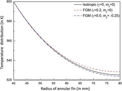
While studying the forward problem, it is insightful to study the effect of various thermal parameters on the heat transfer of fin. Figure 2 shows that the non-dimensional temperature fields monotonically decrease from bore to tip in the radial direction for all the variation of thermal parameters. It can be seen that the local temperature field decreases with the increase in thermo-geometric parameter, N_c. Thermal energy is efficiently transferred from the fin surfaces to environment as large amount of heat is convected when the parameter N_c is increased, and thus, the temperature gradient increases with the increase of N_c. The conductive–radiative parameter, N_r, also has an influence on the variation of the local temperature field. The rate of radiative heat transfer from the fin to the surrounding increases with the increase in N_r. As a result, higher local temperature drop is observed with the increase of N_r. Opposite behaviour can be seen regarding the variation of variable thermal conductivity parameter, γ. The decrease in the value of γ decreases the local temperature distribution. The total thermal conductivity is reduced when the value of γ is reduced. As the thermal resistivity is increasing with the decrease of thermal conductivity, the heat flow through the fin material is obstructed, and hence the reduction in local temperature distribution is observed. The comparison of temperature distribution between isotropic and FGM fin is depicted in Figure 3. In this comparison, the same dimensional parameters as mentioned in Table 1 were taken and the heat generation and surrounding temperature were neglected. The effect of varying the parameters in spatial coordinates (FGM) on the temperature distribution is clearly evident. This effect depends on the relationship of variation of parameters with the spatial coordinate. As the thermal conductivity increases with the radius of the fin, the heat transfer rate also increases. Thus, higher local temperature distribution in FGM fin is observed. On the other hand, more heat is radiated from the fin surface to surrounding when m₂ is negative. As a result, decay in local temperature is seen with the negative value of m₂.

Figure 2. Effect of non-dimensional thermal parameters on non-dimensional temperature distribution.

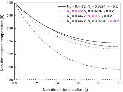
Figure 3. Comparison of temperature distribution in an annular fin made of isotropic material and FGM.

Now, we discuss results related to the inverse problem. The DA following Mirjalili [27] has been employed for optimizing three non-dimensional parameters, N_c, N_r and γ, for a specified temperature field. In one situation, HPM is used as the forward solver in the structure of DA. In another situation, ODE is used as the forward solver in the structure of DA. All the inverse parameters are being simultaneously estimated for the desired temperature field. In this analysis, the desired temperature field is the same as that obtained from the forward solution by considering the non-dimensional parametric values shown in Figure 2.

Table 2 shows the different combination of parameters, N_c, N_r and γ, inversely estimated from seven different runs. The same solution space (listed in Table 2 as the lower and upper bounds of the optimization variables) is used for the first three runs. Different solution spaces are considered in later runs. Figure 4 represents the convergence study of the (a) objective function and the iteration-wise variation of the inverse parameters (b) N_c, (c) N_r and (d) γ. It can be observed that the simulations are converged in the range of 100–250 iterations.

Figure 4. Optimization for inversely estimated of parameters showing (a) convergence histories of the objective function, and iteration-wise variations of (b) N_c, (c) N_r and (d). (a) Convergence histories of the objective function, (b) Iteration-wise variation of N_c, (c) Iteration-wise variation of N_r, (d) Iteration-wise variation of γ.

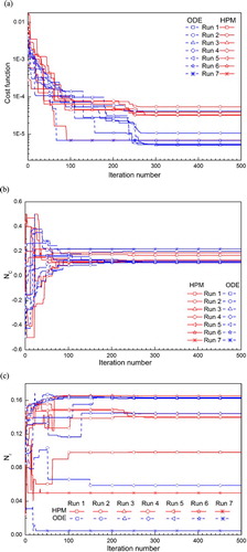
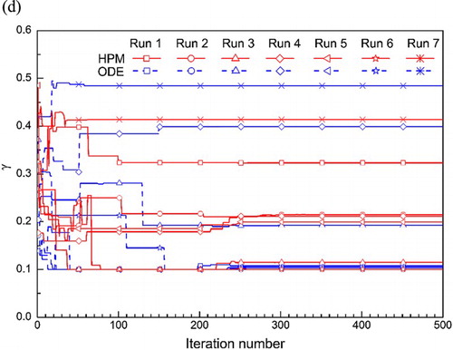
Table 2. Thermal parameters estimated using DA in seven independent runs.

	Inverse based on HPM-based forward solution				Inverse based on ODE-based forward solution				Range of parameters (Nc, Nr, γ)
Run	Nc	Nr	γ	Time (s)	Nc	Nr	γ	Time (s)	Lower bound	Upper bound
R1	0.323	0.098	0.1668	69.7	0.108	0.162	0.107	369.7	0.1, 0.01, −0.5	1.0, 0.5, 0.5
R2	0.215	0.14	0.124	70.89	0.1	0.164	0.108	378.12	0.1, 0.01, −0.5	1.0, 0.5, 0.5
R3	0.114	0.163	0.109	69.76	0.192	0.145	0.121	373.24	0.1, 0.01, −0.5	1.0, 0.5, 0.5
R4	0.212	0.141	0.1253	64.5	0.399	0.059	0.199	360.17	0.1, 0.01, −0.5	0.6, 0.5, 0.5
R5	0.199	0.144	0.121	70.41	0.106	0.163	0.113	373.44	0.1, 0.01, −0.5	0.8, 0.5, 0.5
R6	0.1	0.165	0.1063	71.98	0.103	0.163	0.110	377.65	0.1, 0.01, −0.5	1.2, 0.5, 0.5
R7	0.414	0.05	0.1866	72.36	0.484	0.005	0.218	309.77	0.4, 0.01, −0.5	0.6, 0.5, 0.5

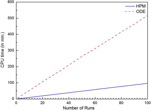
The CPU time for non-stop 100 times inverse simulation considering HPM-based forward solution is compared with the ODE-based forward solution in Figure 5. The result shows that the simulation time for inversely estimated parameters obtained from HPM-based forward solution is much lower (more than five times less) than that of ODE-based forward solution. For this simulation, core i5 pentium-4 with 8 GB ram PC was used.

Figure 5. CPU time against the number of runs for inverse estimation of three parameters (N_c, N_r and γ) considering forward solution of HPM and ODE.

The various combination of inverse parameters obtained after every run of 100 runs is presented in Figure 6. It can be seen that the profile of parameters estimated using DA with HPM forward solver is similar to the parameters estimated using DA with ODE forward solver. Each data point in the plots in Figure 6 represent a unique set of values of the parameters, N_c, N_r and γ, however each data point resulting in the same temperature field.

Figure 6. Variation of parameters (N_c, N_r and γ) obtained in 100 runs of DA algorithm for inverse solution: (a) considering HPM forward solver and (b) considering ODE forward solver.

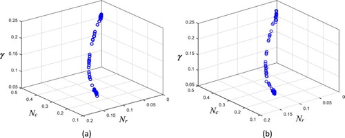
Inverse problems are ill-posed in at least one of the following: existence of solution, uniqueness of solution, stability of solution. In this case, uniqueness of the solution is compromised. Here, we use the inverse approach for the design problem. In a design problem, there may be multiple suitable designs (multiple solutions) and the most suitable solution among them can be identified through consideration of the other design considerations. Thus, Figure 6 has an important implication on the fin design. It shows that the inverse problem of this system is non-unique, i.e. multiple sets of physical parameters can provide a satisfactory solution. Notably, they fall along a certain locus, which represents a minimum locus of the cost function used for optimization. The presence of multiple solutions provides an opportunity of exploitation as a design solution. In an industrial design problem, the thermal properties are an important design consideration but not the only one. Having a pool of feasible solution allows selection of the best-suited parameters according to the other design considerations as well. At the same time, the fact that the solution lies along a certain locus can be used to identify this locus without performing an exhaustive analysis of cost function in the entire solution space. This locus can then be used to generate the empirical insight into the thermal aspect of system design.

To confirm the correctness of the inverse solution, the values of estimated parameters are used in forwarding solver and compared with the given temperature field. Figure 7 shows the reconstructed temperature fields obtained using the parameters of the inverse solution listed in Table 2. The reconstructed temperature fields are compared with the specified temperature field and have found in very good agreement. Table 3 represents the tip temperatures obtained from inversely estimated thermal parameters and compared with the reference tip temperature. The results revealed that the percentage of error in each case is below 1%.

Figure 7. Comparison of forward temperature field and the reconstructed temperature fields obtained from inverse parameters.

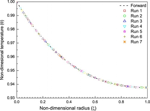
Table 3. Comparisons between the forward and inversely estimated tip temperatures and the percentage of error under the investigation of various combination of thermal parameters (as in Table 2).

	θtip estimated from the inverse parameters of different run
HPM-based θtip	R1	R2	R3	R4	R5	R6	R7
0.93768	0.93763	0.93755	0.93755	0.93755	0.93759	0.93757	0.93755
% of error	0.0053	0.0139	0.0139	0.0139	0.0096	0.1173	0.0139

6. Conclusion

This paper presents the results for temperature distribution of isotropic and FGM material annular fin. In addition to this, the results are also presented for dimensional and non-dimensional temperature field. This temperature field is obtained by solving nonlinear heat transfer equation of a conductive–convective–radiative annular fin using HPM, ODE solver and FEM (using Comsol). And, the results obtained through HPM are in a very good agreement with the results of the ODE solver and FEM. Further, dragon fly optimization technique is successfully applied for inverse estimation of thermal parameters (i.e. N_c, N_r and γ) which are mainly responsible for effects on temperature distribution and performance of the fin. Forward solutions of HPM and ODE are used for inverse estimation of thermal parameters. The temperature distribution obtained from estimated parameters, of both the methods give similar profile. Whereas, HPM takes very less time (i.e. five times less than that of ODE) for inverse estimation of thermal parameters compared to ODE. And, the objective function and estimated parameters converge after 100 iterations, this shows that the convergence rate is fast. The thermal conductivity and emissivity variation with respect to spatial coordinate show significant effects on temperature distribution.

Nomenclature

ri, ro, t	=	inner radius, outer radius and thickness of the fin
δ	=	dimensionless thickness ratio, δ = t/ri
h(T)	=	convective heat transfer coefficient
k(r)	=	thermal conductivity
ko	=	thermal conductivity at the base of the fin
hb, qo	=	convective heat transfer coefficient and internal heat generation at ambient temperature
εs	=	surface emissivity at the surrounding temperature
γ, e	=	parameter describing the linear variation of thermal conductivity and internal heat generation, respectively
m1, m2	=	exponent for the variation of convective heat transfer coefficient and emissivity
Nc	=	non-dimensional thermo-geometric parameter, (2hbri2/kot)0.5
Nr	=	non-dimensional conduction-radiation parameter, ($2{r_i}^2\sigma {\epsilon }_s{T_b}^3/k_{o}t$)
G	=	non-dimensional heat generation parameter, G = qori2/koTb
EG	=	non-dimensional parameter describing the variation of heat generation
Tb	=	base temperature of the fin
Ta	=	ambient temperature
Ts	=	surrounding temperature
ξ	=	non-dimensional radius of fin, ξ = (r−ri)/ri
R	=	non-dimensional outer radius, R = ro/ri
θ	=	non-dimensional temperature, θ = T/Tb
θa	=	non-dimensional convective environment temperature, θa = T/Tb
θs	=	non-dimensional surrounding temperature for radiation, θs = T/Tb
p	=	embedding parameter
$\mathrm{\Re }\left(\xi \right)$	=	objective function
P	=	number of measurement points

Disclosure statement

No potential conflict of interest was reported by the authors.

References

- Kraus AD. Aziz A, Welty J. Extended surface heat transfer. Hoboken (NJ): John Wiley and Sons; 2001.
- Aksoy IG. Thermal analysis of annular fins with temperature-dependent thermal properties. Appl Math Mech Engl Ed. 2013;34(11):1349–1360.
- Sadri S, Raveshi MR, Amiri S. Efficiency analysis of straight Fin with variable heat transfer coefficient and thermal conductivity. J Mech Sci Tech. 2012;26(4):1283–1290. doi: 10.1007/s12206-012-0202-4
- Campo A, Wolko HS. Optimum rectangular radiative fins having temperature-variant properties. J Spacecraft Rockets. 1973:10(12):811–812. doi: 10.2514/3.61975
- Lesnic D, Heggs PJ. A decomposition method for power-law fin-type problems. Int Commun Heat Mass Transf. 2004:31:673–682 doi: 10.1016/S0735-1933(04)00054-5
- Khan WA, Aziz A. Transient heat transfer in a functionally graded convecting longitudinal fin. Heat Mass Transf. 2012;48:1745–1753. doi: 10.1007/s00231-012-1020-z
- Aziz A, Torabi M, Zhang K. Convective–radiative radial fins with convective base heating and convective–radiative tip cooling: homogeneous and functionally graded materials. Energy Convers Manag. 2013;74:366–376. doi: 10.1016/j.enconman.2013.05.034
- Hassanzadeh R, Pekel H. Heat transfer enhancement in annular fins using functionally graded material. Heat Trans Asian Res. 2013;42(7):603–617. doi: 10.1002/htj.21053
- Peng XL, Li, XF. Thermoelastic analysis of functionally graded annulus with arbitrary gradient. Appl Math Mech Engl Ed. 2009:30(10):1211–1220.
- Aziz A, Rahman MM. Thermal performance of a functionally graded radial Fin. Int J Thermophys. 2009;30:1637–1648. doi: 10.1007/s10765-009-0627-x
- Karkhin VA, Plochikhine VV, Bergmann HW. Solution of inverse heat conduction problem for determining heat input, weld shape, and grain structure during laser welding. Sci Technol Weld Joining. 2002;7:224–231. doi: 10.1179/136217102225004202
- Groetsch CW. Inverse problems: activities for undergraduates. Cambridge: Cambridge University Press; 1999.
- Pehlivanoglu YV. Direct and indirect design prediction in genetic algorithm for inverse design problems. Appl Soft Comput. 2014;24:781–793. doi: 10.1016/j.asoc.2014.08.018
- Chen HT, Hsu WL. Estimation of heat transfer coefficient on the fin of annular-finned tube heat exchangers in natural convection for various fin spacings. Int J Heat Mass Transf. 2007;50:1750–1761. doi: 10.1016/j.ijheatmasstransfer.2006.10.021
- Słota D. Using genetic algorithms for the determination of an heat transfer coefficient in three-phase inverse Stefan problem. Int Commun Heat Mass Transf. 2008;35:149–156. doi: 10.1016/j.icheatmasstransfer.2007.08.010
- Hetmaniok E, Nowak I, Słota D, et al. Application of the homotopy perturbation method for the solution of inverse heat conduction problem. Int Commun Heat Mass Transf. 2012;39:30–35. doi: 10.1016/j.icheatmasstransfer.2011.09.005
- Yu GX, Sun J, Wang HS, et al. Meshless inverse method to determine temperature and heat flux at boundaries for 2D steady-state heat conduction problems. Exp Therm Fluid Sci. 2014:52:156–163. doi: 10.1016/j.expthermflusci.2013.09.006
- Mohasseba S, Moradi M, Sokhansefat T, et al. A novel approach to solve inverse heat conduction problems: coupling scaled boundary finite element method to a hybrid optimization algorithm. Engg Anal Bound Elem 2017:84:206–212. doi: 10.1016/j.enganabound.2017.08.018
- Yang CY. Direct and inverse solutions of the two-dimensional hyperbolic heat conduction problems. App Math Model 2009:33:2907–2918. doi: 10.1016/j.apm.2008.10.001
- Ozisik MN, Orlande HRB. Inverse heat transfer fundamentals and applications. New York: Taylor & Francis; 2000.
- Lesnic D, Elliott L. The decomposition approach to inverse heat conduction. J Math Anal Appl. 1999:232:82–98. doi: 10.1006/jmaa.1998.6243
- Hajabdollahi F, Rafsanjani HH, Hajabdollahi Z, et al. Multi-objective optimization of pin fin to determine the optimal fin geometry using genetic algorithm. Appl Math Model. 2012;36:244–254. doi: 10.1016/j.apm.2011.05.048
- Bamdad K, Ashorynejad HR. Inverse analysis of a rectangular fin using the lattice Boltzmann method. Energy Convers Manag. 2015;97:290–297. doi: 10.1016/j.enconman.2015.02.075
- Chang YC, Chen WH, Lee CY, et al. Simulated annealing based optimal chiller loading for saving energy. Energy Convers Manag. 2006;47:2044–2058. doi: 10.1016/j.enconman.2005.12.022
- Das R, Mallick A, Ooi KT. A fin design employing an inverse approach using simplex search method. Heat Mass Transf. 2013;49:1029–1038. doi: 10.1007/s00231-013-1146-7
- Lee HL, Chang WJ, Chen WL, et al. Inverse heat transfer analysis of a functionally graded fin to estimate time-dependent base heat flux and temperature distributions. Energy Convers Manag. 2012;57:1–7. doi: 10.1016/j.enconman.2011.12.002
- Mirjalili S. Dragonfly algorithm: a new meta-heuristic optimization technique for solving single-objective, discrete, and multi-objective problems. Neural Comput Appl. 2016;27:1053–1073. doi: 10.1007/s00521-015-1920-1
- He JH. Homotopy perturbation technique. Comput Methods Appl Mech Engg. 1999;178:257–262. doi: 10.1016/S0045-7825(99)00018-3
- He JH. Homotopy perturbation technique: a new nonlinear analytical technique. Appl Math Comput. 2003;135:73–79.
- Shakeri F, Dehghan M. Inverse problem of diffusion equation by He’s homotopy perturbation method. Phys Scr 2007;75(4):551–556. doi: 10.1088/0031-8949/75/4/031
- Mallick A, Ghosal S, Sarkar PK, et al. Homotopy perturbation method (HPM) for thermal stresses in an annular fin with variable thermal conductivity. J Therm Stresses. 2015;38:110–132. doi: 10.1080/01495739.2014.981120
- Ranjan R, Mallick A. An efficient unified approach for performance analysis of functionally graded annular fin with multiple variable parameters. Therm Eng. 2018:65:614–626 (in press). doi: 10.1134/S0040601518090082
- Comsol Multiphysics® 4.3., Burlington (MA): 2012.
- Shampine LF, Kierzenka J, Reichelt MW. Solving boundary value problems for ordinary differential equations in MATLAB with bvp4c. Tutorial Notes. 2000; 2000:1–27.
- Chiu CH, Chen CK. Thermal stresses in annular fins with temperature dependent conductivity under periodic boundary condition. J Thermal Stresses 2002;25:475–492. doi: 10.1080/01495730252890195