Static damage identification in beams by minimum constitutive relation error

ABSTRACT

A novel static identification approach to beam damage is presented. It is based on the minimum constitutive relation error (CRE) principle where the exact stiffness, the exact displacement and the exact bending moment are shown to make the CRE functional minimal. For practical implementation, two cases regarding full-field displacement measurements and finite-point displacement data, respectively, are considered. For full-field displacement measurements, the CRE functional is directly treated as the objective functional while in case of finite-point measurement data, the CRE functional along with additional penalty terms for treatment of the finite-point displacement measurements is defined as the objective functional. Multiple loads and associated sets of measurements are also considered to improve the identifiability and robustness of the procedure. Convergence is finally verified through numerical examples.

KEYWORDS:

• Damage identification
• static measurements
• constitutive relation error (CRE)
• full-field displacement measurement
• finite-point displacement measurement

SUBJECT CLASSIFICATION CODES:

• 70J10
• 74S05

1. Introduction

Damage can arise in structures due to operational incidents, extreme events and/or aggressive environmental conditions. It mainly causes a loss of structural stiffness which may affect the safety, integrity, serviceability and operation of structures. Thus, establishment of the structural health monitoring (SHM) system that provides damage and safety information for preventive maintenance, inspection and repair of structures becomes essential. Indeed, a reliable and effective non-destructive damage identification approach is always the core ingredient of the SHM [1].

There are several conventional, experimental and local approaches that are able to directly identify the damage. The simplest one is visual inspection; however, it is often difficult and even impossible to work well since there may be damage scenarios that are not visible [2]. Other approaches, such as ultrasonic testing, radiography and thermal analysis, require the damaged region to be known a priori and accessible for testing, which cannot be guaranteed in most cases [1]. Hence, global approaches accounting for global behaviour of the damaged region are developed to overcome the difficulties.

Generally, global damage detection approaches are devoted to the identification of damage location and level based on the procedure in which the responses caused by external excitations are measured from dynamic or static tests [3] and thereafter, the damage is often identified indirectly through numerical manipulations. A direct consequence of damage is the decrease in local stiffness, and therefore damage, regarded as changes in stiffness, can be detected using changes in dynamic or static characteristics since response characteristics are functions of structural stiffness. This has been the key idea of many extant global approaches [1–5].

In fact, considering the nature of the measured data, global approaches can be classified into two categories: dynamic and static procedures. Due to the convenience in dynamic data measurements, a much larger number of damage identification approaches have been developed based on dynamic tests [6–12]. On the other hand, for certain types of structures, like beam structures, static tests can be performed as easily as dynamic tests. Under this circumstance, the static equilibrium equation is only related to the structural stiffness, and static displacement and strain measurements can be obtained accurately, rapidly and cheaply; while approaches based on dynamic tests often require additional knowledge of mass and damping information, that is to say, the dynamic identification procedure is often complicated due to the uncertainties coming from mass and damping measurements. In spite of the fact, relatively less attention has been paid to static damage identification. Banan and Hjelmstad [13,14], Viola and Bocchini [15] conducted static parameter identification through minimizing certain error functions, like least squares fitting errors in displacements or equilibrium equations, based on finite element models. Di Paola and Bilello [2] identified damage in beams through an integral equation. Ghrib et al. [16] investigated the efficiency of two computational procedures – equilibrium gap formulation and minimization of a data-discrepancy functional – for damage detection using static responses. Avril and Pierron [17] proposed a virtual field method for the identification of constitutive parameters. Yang and Sun [18], Rezaiee-Pajand et al. [19] localized and quantified structural damage through sensitivity analysis of the stiffness to finite element equilibrium equations. Caddemi and Greco [20], Abdo [3], Bakhtiari-Nejad et al. [21] analysed the influence of measurement noises, number and spatial distribution of measured data and character of load cases.

In the present paper, damage identification is performed based on static test data through a minimum constitutive relation error (CRE) procedure which is quite different from the error function approaches in [13–15,22]. The idea is enlightened by a recent variational theory of Geymonat and Pagano [23] for inverse parameter identification that the CRE function is convex and its minimization can lead to a well-posed problem. As they pointed out, constitutive parameters and stresses can be identified through minimization of the CRE as long as displacement measurements are readily acquired under given loads. The conclusion reached by the theory is very attractive and as a first attempt to implement the theory, a constitutive equation gap method has been proposed very recently by Florentin and Lubineau [24–27] for parameter identification in plane elasticity problems. However, as indicated in the theory, the complete and comprehensive application requires the full-field/global displacement measurements along with a complementary-energy-based solver for stresses which is not yet applicable to general two- and three-dimensional problems [28,29]. Notwithstanding, the method is quite tailored for beam structures in the following two aspects:

1. global displacement measurements are easily available, and

2. the standard force method [30] based on the minimum complementary energy principle is easily conducted and it often requires substantially less degrees of freedom than conventional displacement-based finite element models.

That is to say, the minimum CRE theory is completely applicable to damage identification in beam structures, to which this paper is just devoted. Considering that getting the measurement data is of vital importance for practical identification and different measurement techniques often correspond to different identification procedures, a number of commonly-used and developing measurement techniques and their recent development are additionally reviewed in what follows.

Traditionally, for static measurements, displacements including deflections and slopes of beams are measured at finite points using linear variable-differential transformers(LVDT) [16]reliable up to 10⁻⁶ mm [31] accuracy and global positioning systems(GPS) [32,33], with absolute errors down to a few millimetres in practice. For damage identification corresponding to these finite-point measurement techniques, the accuracy of identification results depends mainly on the amount and locations of the sensors.

On the other hand, with fast development of computer-based technologies and digital imaging devices, laser and other light sources, optical-based measurement techniques [34]open up a new possibility in quasi-continuous measurement of structures at an affordable cost; these include (but are not limited to) the digital image processing techniques [35], the laser scanning [36,37] and the interferometry [38]. Particularly, the digital image processing techniques, such as digital image correlation [39], close-range digital photogrammetry [40], image edge detection [41], optical flow method/principle [42,43], have exhibited their powerful measurement abilities in various experiments. Results even showed that the relative error between the displacements measured by these techniques and the exact value scan be less than 0.5% [44]. In addition, prior researches have shown that the full-field displacements could be appropriately rebuilt through a sufficient number of displacement data along with some suitable data pre-processing algorithms [45]. For more optical-based measurement techniques in both static and dynamic engineering applications, refer to [38,41,42,46–53].

In this paper, damage identification in beams is performed using either the finite-point measurements by the traditional LVDT or the quasi-continuous measurements by the optical-based techniques. The primary objective is to identify the damaged stiffness $k\in \mathcal{C}$ as well as bending moment $M\in \mathrm{\Im }$, under the full-field displacement measurements $w\in \mathcal{U}$, e.g. obtained by optical-based techniques and the respective static loading conditions $\mathrm{\Im }$ where $\mathcal{C}$, $\mathcal{U}$, $\mathrm{\Im }$ represent the admissible material, displacement and bending moment spaces, respectively. The basic inverse identification problem reads: find $(k,M)\in \mathcal{C}-\times \mathrm{\Im }$ with given $w\in \mathcal{U}$, which is a reverse of the forward problem: find $(w,M)\in \mathcal{U}-\times \mathrm{\Im }$ with known $k\in \mathcal{C}$. Evidently, by solving the inverse problem, one can not only identify the damage, but also reconstruct the stiffness and bending moment distribution. Moreover, the objective is also enriched to tackle damage identification using finite-point displacement measurements. By this way, the static damage identification procedure becomes more adjustable to traditional measurement techniques, e.g. the LVDT for which finite-point displacement measurements are often obtained.

The remainder of the paper is organized as follows. The inverse identification problem for a Bernoulli-Euler beam model is simply introduced in Section 2. In Section 3, the minimum CRE principle for inverse identification is presented for full-field displacement measurements and then, the modification is invoked to cope with finite point measurements. Practical implementation and convergence of the proposed approach are discussed elaborately in Section 4. Numerical tests are performed in Section 5 and final conclusions are drawn in Section 6.

2. Problem statement

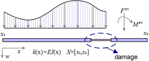
Consider a one-dimensional Bernoulli-Euler beam defined in interval $X=[x_s,x_e]$ as shown in Figure 1. The flexural stiffness of the beam is assumed to be $k\left(x\right)=EI\left(x\right)$. Loading conditions are distributed loads $q\left(x\right)$ and concentrated loads $F^{ex},M^{ex}$ along with boundary displacements $w_p$ on the prescribed displacement boundary $\mathrm{\Sigma }$. In this beam model, the bending moment $M$ is directly related to the curvature through the constitutive relation $M=k{\theta }^{\mathrm{\prime }}=k{w}^{\mathrm{\prime \prime }}$ and the shear force $V$ is given by $V=M^{\mathrm{\prime }}$. For general equilibrium, $V^{\mathrm{\prime }}=M^{\mathrm{\prime \prime }}=q\left(x\right)$ and $V,M$ should be in equilibrium with concentrated loads. The beam model can be described as a combination of the following three parts:

• Kinematic constraints (1) $\mathcal{U}=\{w\in H^2(X):w=w_p\text{ on }\mathrm{\Sigma }\}$(1)

• Equilibrium equations

Figure 1. A Bernoulli-Euler beam with damage.

Find bending moment $M\in \mathrm{\Im }$ with (2) $\mathrm{\Im }=\{M:V=M^{\mathrm{\prime }},M^{\mathrm{\prime \prime }}=q(x),V\text{ and }M\text{ are in equilibrium with }{F}^{ex}\text{ and }{M}^{ex}\}$(2) or (3) $\mathrm{\Im }=\{M\in L_2(X):{\int }_{X}M{v}^{\mathrm{\prime \prime }}\text{d}x={\int }_{X}q\left(x\right)v\text{d}x+\sum \left(F^{ex}v\right(x^{ex})+M^{ex}{v}^{\mathrm{\prime }}(x^{ex}\left)\right),\mathrm{\forall }v\in {\mathcal{U}}_0\}$(3) with $x^{ex}$ denoting the position where concentrated loads $F^{ex},M^{ex}$ are enforced and ${\mathcal{U}}_0$ the homogeneous part of $\mathcal{U}$;

• Constitutive relation (4) $M=k{w}^{\mathrm{\prime \prime }}$(4) with $k\in \mathcal{C}-=\{k\in L_2(X):\mathrm{\exists }0<c_0<C_0,\text{ such that }{c}_0\le k(x)\le C_0\}$ representing a positive and bounded stiffness field.

  Generally, $\mathcal{U}$,$\mathrm{\Im }$,$\mathcal{C}-$ that will be used frequently in what follows are called the spaces of (kinematically) admissible displacement field, (statically) admissible bending moment field and (constitutively) admissible elastic stiffness field, respectively.

3. The minimum CRE principle for inverse identification

3.1. CRE functional

Consider an admissible solution trio $(\overline{w},\overline{M},\overline{k})$ which satisfies (5) $\overline{w}\in \mathcal{U},\overline{M}\in \mathrm{\Im },\overline{k}\in \mathcal{C}$(5) It is easily known that if the constitutive relation (4) is additionally satisfied, the solution trio would be the exact solution of the Bernoulli–Euler beam model. Thus, to measure the distance of the admissible solution trio to the exact solution trio in an energy expression, an error in constitutive relation is introduced (6) $e_{CRE}(\overline{w},\overline{M},\overline{k})=\frac{1}{2}{\int }_X\frac{{(\overline{M}-\overline{k}{\overline{w}}^{\mathrm{\prime \prime }})}^2}{\overline{k}}\text{d}x$(6) which is termed the constitutive relation error (CRE) [54,55] (or constitutive equation gap (CEG) [24]). For the convenience of presentation, only one-dimensional Bernoulli–Euler beam is discussed in this research. The extension of the basic CRE term to other structures, e.g. frames, is straightforward. Particularly, the expression of CRE for the more general Timoshenko beam considering the influence of transverse shear effects is formulated in the Appendix.

3.2. Identification through minimum CRE

In practice, damage identification approaches appear to be limited with respect to certain displacement measurement techniques. Herein, two cases regarding full-field displacement measurements and finite-point displacement data, respectively, are considered within the framework of the minimum CRE theory. For the first case using full-field displacement measurements, the CRE functional (6) is directly treated as the objective functional and the parameter identification approach is referred to as the min-CRE approach; while in case of finite-point measurement data, the CRE functional along with additional penalty terms for treatment of the finite-point displacement measurements are defined as the objective functional. The second identification case is more applicable and can be viewed as an extension of the first identification case. Therefore, the identification approach involved in the second case is referred to as the modified min-CRE approach.

3.2.1. Min-CRE approach

Assume that the spaces $\mathcal{C}$,$\mathcal{U}$ and $\mathrm{\Im }$ for search of the stiffness $k$, displacement $w$ and the bending moment $M$, respectively, are already known. Then, identification of the stiffness $k$ as well the bending moment $M$ from the full-field displacement data $\hat{w}$ pertains to the following minimization of the CRE functional (6), i.e. (7) $(M,k)=\arg \underset{\overline{M}\in \mathrm{\Im },\overline{k}\in \mathcal{C}}{min}F(\overline{M},\overline{k});F(\overline{M},\overline{k}):=e_{CRE}(\overline{M},\overline{k},\hat{w})$(7) which is known as the minimum CRE principle [23] for inverse identification. To proceed further, it is necessary to clarify some important properties of the CRE function $F(\cdot ,\cdot ,\cdot )$.

Theorem 3.1:

The following properties for $F(\cdot ,\cdot )$ on compact spaces $\mathrm{\Im }\times \mathcal{C}$ hold:

1. $F(\overline{M},\overline{k})\ge 0$,$\mathrm{\forall }(\overline{M},\overline{k})\in \mathrm{\Im }\times \mathcal{C}\times \mathcal{U}$.

2. $F(\overline{M},\overline{k})=0$ if and only if the constitutive relation $\overline{M}=\overline{k}\widehat{w^{\mathrm{\prime \prime }}}$ is verified.

3. The functional $F(\cdot ,\cdot )$ is convex on $\mathrm{\Im }\times \mathcal{C}$.

4. The convexity of $F(\cdot ,\cdot )$ on $\mathrm{\Im }\times \mathcal{C}$ guarantees the existence of the minimizer to problem (7). Then, if $\mu (x\in X:\widehat{w^{\mathrm{\prime \prime }}}(x)=0)=0$ with $\mu (\cdot )$ denoting the Lebesgue measure, the minimizer must lie in ${\mathrm{\Im }}^{\ast }\times \mathcal{C}$ with ${\mathrm{\Im }}^{\ast }=\{M\in \mathrm{\Im }:\mu (x\in X:M\left(x\right)=0)=0\}$ and moreover, $F(\cdot ,\cdot )$possesses separately strict convexity on ${\mathrm{\Im }}^{\ast }\times \mathcal{C}$.

Detailed proof of the Theorem 3.1 is given in the Appendix. According to Theorem 3.1, it is seen that the damaged stiffness is identifiable through the minimum CRE principle in beams. Theoretically, the complete and unique identification of the damage requires some extra conditions on the static measurements – which are inherent in the context of inverse problems (see Remark A1 in the Appendix) – including the deforming condition $\mu \left(\widehat{w^{\mathrm{\prime \prime }}}\right(x)=0,x\in X)=0$ such that $F(\cdot ,\cdot )$ becomes strictly convex in the vicinity of the minimizer.

In practice, using more than one set of static measurements could improve the identifiability and robustness of the identification procedure and provide a remedy for possible unidentifiability of the proposed approach [31,56]. To this end, the objective functional as well as the identification procedure becomes, (8) $\begin{array}{l}(M^{\left(1\right)},M^{\left(2\right)},\dots ,k)=\arg \underset{{\overline{M}}^{\left(j\right)}\in {\mathrm{\Im }}^{\left(j\right)},\overline{k}\in \mathcal{C}}{min}F({\overline{M}}^{\left(1\right)},{\overline{M}}^{\left(2\right)},\dots ,\overline{k});\\ F({\overline{M}}^{\left(1\right)},{\overline{M}}^{\left(2\right)},\dots ,\overline{k}):=\sum _j{r}_j{e}_{CRE}({\overline{M}}^{\left(j\right)},\overline{k},{\hat{w}}^{\left(j\right)})\end{array}$(8) where ${\hat{w}}^{\left(j\right)}$ denotes the jth set of full-field displacement data resulting from the loading condition ${\overline{M}}^{\left(j\right)}\in {\mathrm{\Im }}^{\left(j\right)}$ and $r_j\ge 0$ is the corresponding weighting coefficient and $\sum _j{r}_j=1$. The selection of weighting coefficient $r_j$ is determined by the reliability of practical measurements: if $(w_{\mathrm{m}},{\mathrm{\Im }}_{\mathrm{m}},{\mathcal{U}}_{\mathrm{m}})$ is more reliable than $(w_n,{\mathrm{\Im }}_n,{\mathcal{U}}_n)$, $r_{\mathrm{m}}$ would be selected to be greater than $r_{\mathrm{n}}$; else it would be otherwise. Generally, $r_{\mathrm{m}}$ and $r_{\mathrm{n}}$ are taken equally. It is evidently seen that as long as $\sum _j{r}_j{\left({w^{\mathrm{\prime \prime }}}_j\right)}^2\ne 0$ on $X_i,\mathrm{\forall }i=1,2,\dots ,n$, the constitutive-relation step for $k_i$ can proceed.

3.2.2. Modified min-CRE approach

In most cases, finite-point displacement measurements rather than full-field displacement measurements are available. Herein, an additional penalty term is introduced into the constitutive relation error function(6) in order to weakly enforce the finite-point displacement measurements and account for the different levels of measurement noise of these data. Let $\{{\hat{w}}_i,i\in \mathrm{\wp }\}$ be the measured finite-point displacement data on the set of points $\{i\in \mathrm{\wp }\}$ and then, a new objective functional as well as a new parameter identification formulation is given as follows. (9) $\begin{array}{l}{F}_{mod}(\overline{M},\overline{k},\overline{w}):=e_{CRE}(\overline{M},\overline{k},\overline{w})+\sum _{i\in \mathrm{\wp }}\frac{A_i}{2}|{\overline{w}}_i-{\hat{w}}_i{|}^2\\ (M,w,k)=\arg \underset{\overline{M}\in \mathrm{\Im },\overline{w}\in \mathcal{U},\overline{k}\in \mathcal{C}}{min}{F}_{mod}(\overline{M},\overline{k},\overline{w});\end{array}$(9) where $w_i$ is the displacement $w$ at point $i$ and $\{A_i>0,i\in \mathrm{\wp }\}$ represent the penalty factors. Practically, values of $\{A_i>0,i\in \mathrm{\wp }\}$ could be tuned according to the confidence of the corresponding displacement data: $A_i\to +\mathrm{\infty }$ means completely trust of this data, while $A_i\to 0$ means completely untrusted. In the following examples, $A_i$ is chosen based on experience. Again, in the case of multiple sets of static data, the parameter identification can read, (10) $\begin{array}{l}(M^{\left(1\right)},w^{\left(1\right)},M^{\left(2\right)},w^{\left(2\right)},\dots ,k)=\arg \underset{{\overline{M}}^{\left(j\right)}\in {\mathrm{\Im }}^{\left(j\right)},{\overline{w}}^{\left(j\right)}\in {\mathcal{U}}^{\left(j\right)},\overline{k}\in \mathcal{C}}{min}\\ F_{mod}({\overline{M}}^{\left(1\right)},{\overline{w}}^{\left(1\right)},{\overline{M}}^{\left(2\right)},{\overline{w}}^{\left(2\right)},\dots ,\overline{k});\\ F_{mod}({\overline{M}}^{\left(1\right)},{\overline{w}}^{\left(1\right)},{\overline{M}}^{\left(2\right)},{\overline{w}}^{\left(2\right)},\dots ,\overline{k})\\ :=\sum _j{r}_j\left[e_{CRE}({\overline{M}}^{\left(j\right)},\overline{k},{\overline{w}}^{\left(j\right)})+\sum _{i\in \mathrm{\wp }}\frac{A_i}{2}{|{{\overline{w}}_i}^{\left(j\right)}-{{\hat{w}}_i}^{\left(j\right)}|}^2\right]\end{array}$(10) where ${\mathrm{\Im }}^{\left(j\right)},{\mathcal{U}}^{\left(j\right)}$ represents the loading and prescribed displacement boundary conditions for the jth set of static measurement, ${{\hat{w}}_i}^{\left(j\right)}$ is the corresponding measurement displacement at point i and $r_j$ is the weight.

In what follows, specific algorithms will be elaborately designed to solve the minimization problems (7)–(10).

4. Practical implementation

Section 3 gave the theoretical view that the damaged stiffness can be identified through the minimum CRE principle. In this section, numerical algorithms for the min-CRE approach and the modified min-CRE approach are to be developed.

4.1. Min-CRE approach

In Theorem 3.1, the CRE function is shown to be convex and hence, separately convex on $\overline{M}$ and $\overline{k}$. Thus, for practical implementation, a two-step substitution algorithm is developed as follows:

Firstly, minimization of the CRE function over $\overline{M}$ by virtue of Equation (6) and through integration by parts leads to (11) ${\int }_X\frac{\overline{M}}{\overline{k}}\delta \overline{M}dx={\int }_X{w}^{\mathrm{\prime \prime }}\delta \overline{M}dx={\sum }_p({\theta }_p\delta \overline{M}{|}_p-w_p\left(\delta \overline{M}{)}^{\mathrm{\prime }}{|}_p\right)$(11) where the subscript p indicates the prescribed displacement boundary condition and $\delta \overline{M}$ is any arbitrary variation. Obviously, Equation (11) embodies the minimum complementary energy principle (12) $\begin{array}{l}\overline{M}=Force\mathrm{\_}Method(\overline{k},\mathrm{\Im },\mathcal{U})\\ :=\arg \underset{\overline{M}\in \mathrm{\Im }}{min}\left\{\frac{1}{2}{\int }_X\frac{{\overline{M}}^2}{\overline{k}}\text{d}x-{\sum }_p({\theta }_p\overline{M}{|}_p-w_p\left(\overline{M}{)}^{\mathrm{\prime }}{|}_p\right)\right\}\end{array}$(12) This step is called the force-method step. For numerical details on the force method, one can refer to [30].

Secondly, minimization of the CRE over $\overline{k}$ gives (13) ${\int }_X\left\{\frac{{\overline{M}}^2}{{\overline{k}}^2}-{\left(w^{\mathrm{\prime \prime }}\right)}^2\right\}\delta \overline{k}\text{d}x=0.$(13) Practically, it is sufficient to assume that the stiffness $\overline{k}$ is piecewise constant, that is to say, (14) $\begin{array}{l}X={\cup }_{i=1}^N{X}_i,\mathrm{\forall }1\le i\ne j\le N,X_i\text{ and }{X}_j\text{ are non-overlapping,}\\ \overline{k}\left(x\right)=\{{\overline{k}}_i,x\in X_i\}\end{array}$(14) where $N$ is the number of non-overlapping pieces, or elements. Equation (13) means that the equation in the parenthesis must be zero at every point due to any variation of stiffness. Under the piecewise constant assumption of the stiffness and due to any variation of piecewise constant stiffness, Equation (13) is reduced to (15) $\sum _i{\int }_{X_i}\left\{\frac{{\overline{M}}^2}{{\overline{k}}_i^2}-{\left(w^{\mathrm{\prime \prime }}\right)}^2\right\}\delta {\overline{k}}_i\text{d}x=0\iff {\int }_{X_i}\left\{\frac{{\overline{M}}^2}{{\overline{k}}_i^2}-{\left(w^{\mathrm{\prime \prime }}\right)}^2\right\}\text{d}x=0,i=1,2,\dots ,N$(15) and then, one has (16) ${\overline{k}}_i=\sqrt{\frac{{\int }_{X_i}{\overline{M}}^2\text{d}x}{{\int }_{X_i}{\left(w^{\mathrm{\prime \prime }}\right)}^2\text{d}x}},i=1,2,\dots ,N$(16) It turns out that Equation (16) looks like the direct use of the constitutive relation in Equation (4). Thus, this step is named the constitutive-relation step.

After integration of both Equations (12) and (16), a two-step iterative algorithm for the min-CRE approach is established for its convenience to solve sets of equations. Actually, the two-step substitution algorithm is designed for solution of the discrete version of the problem (8); that is (17) $(M_h,k_h)=\arg \underset{{\overline{M}}_h\in \mathrm{\Im },{\overline{k}}_h\in {\mathcal{C}}_h}{min}F({\overline{M}}_h,{\overline{k}}_h)$(17) where ${\mathcal{C}}_h=\{k\in \mathcal{C}:k\text{ is constant in }{X}_i,i=1,2,\dots ,N\}$ is a compact subspace of $\mathcal{C}$. Finally, as closure of this subsection, the two-step substitution algorithm will be shown to converge for problem (17).

Theorem 4.1:

Assume that the problem (17) has a unique minimizer $(M_h,k_h)$ and $F(\cdot ,\cdot )$ is strictly convex in the vicinity of $(M_h,k_h)$, then, the two-step substitution algorithm will converge to the exact solution.

The specific proof is exhibited in the Appendix. The convergence theorem above is for the min-CRE approach using only one set of static measurement data, nevertheless, it can be easily extended to the min-CRE approach with more than one set of static measurements and the modified-CRE approach; these will not be specified any more. As regards the case of more than one set of static measurements, a similar algorithm can be established as shown in Table 1. It should be noted that the initial value of stiffness $k^0$ should be chosen based on the intact structure. This value is reasonably close to the damaged stiffness and thus to some extent guarantees the convergence to the satisfied results of this problem.

Table 1. A two-step substitution algorithm for min-CRE approach under multiple sets of static measurements w.

Given the initial stiffness $k^0$ and the initial bending moment $M^{\left(1\right)0},M^{\left(2\right)0},\dots$, i.e.

$\begin{array}{l}{M}^{\left(1\right)0}=Forc{e}_{-}Method(k^0,{\mathrm{\Im }}^{\left(1\right)},{\mathcal{U}}^{\left(1\right)}),\\ M^{\left(2\right)0}=Forc{e}_{-}Method(k^0,{\mathrm{\Im }}^{\left(2\right)},{\mathcal{U}}^{\left(2\right)}),\\ \dots \end{array}$

Successively determine $\left(k^{n+1},M^{\left(1\right)n+1},M^{\left(2\right)n+1},\dots \right)$ from $\left(k^n,M^{\left(1\right)n},M^{\left(2\right)n},\dots \right)$ by the following two steps,

step 1: $k^{n+1}=\{\sqrt{\frac{{\int }_{X_i}\sum _j{r}_j{\left(M^{\left(j\right)n}\right)}^{2}dx}{{\int }_{X_i}\sum _j{r}_j{\left({w^{\left(j\right)}}^{\mathrm{\prime \prime }}\right)}^{2}dx}},x\in X_i,i=1,2,\dots ,N\}$,

step 2: $\begin{array}{l}{M}^{\left(1\right)n+1}=Forc{e}_{-}Method(k^{n+1},{\mathrm{\Im }}^1,{\mathcal{U}}^1),\\ M^{\left(2\right)n+1}=Forc{e}_{-}Method(k^{n+1},{\mathrm{\Im }}^2,{\mathcal{U}}^2),\\ \dots \end{array}$

Test of convergence with given error tolerance $\text{TOL}$,

$\sqrt{\frac{{\int }_X{(k^{n+1}-k^n)}^{2}dx}{{\int }_X{\left(k^0\right)}^{2}dx}}+\sqrt{\frac{{\int }_X{(M^{\left(1\right)n+1}-M^{\left(1\right)n})}^{2}dx}{{\int }_X{\left(M^{\left(1\right)0}\right)}^{2}dx}}+\sqrt{\frac{{\int }_X{(M^{\left(2\right)n+1}-M^{\left(2\right)n})}^{2}dx}{{\int }_X{\left(M^{\left(2\right)0}\right)}^{2}dx}}+\dots \le \text{TOL}$

4.2. Modified min-CRE approach

Turning to the modified CRE functional (9), it is found that minimization over $\overline{k}$ would result in the same constitutive-relation step (16) with those in the min-CRE approach. The difference lies in the introduction of a new unknown quantity $w$. Minimization of the CRE functional (9) over $\overline{M}$ and $\overline{w}$ yields (18) ${\int }_X\delta \overline{M}\left(\frac{\overline{M}}{\overline{k}}-\overline{w^{\mathrm{\prime \prime }}}\right)\text{d}x+{\int }_X\delta \overline{w^{\mathrm{\prime \prime }}}\left(\overline{k}\overline{w^{\mathrm{\prime \prime }}}-\overline{M}\right)\text{d}x+\sum _{i\in \mathrm{\wp }}{A}_i\delta {\overline{w}}_i({\overline{w}}_i-{\hat{w}}_i)=0$(18) where $\overline{M}={\overline{M}}_r+{\hat{M}}_P$ with ${\overline{M}}_r={\mathit{N}}_{\mathit{r}}{\overline{\mathit{F}}}_{\mathit{r}}$ being the bending moment produced by the unknown redundant forces $\overline{{\mathit{F}}_{\mathit{r}}}$ and the corresponding shape functions ${\mathit{N}}_{\mathit{r}}$, and ${\hat{M}}_p={\mathit{N}}_p{\hat{\mathit{F}}}_p$ the bending moment caused by the given external loads ${\hat{\mathit{F}}}_p$ and the corresponding shape functions ${\mathit{N}}_{\mathit{p}}$. Indeterminate structures have more unknowns that can be directly solved using equilibriums. The extra unknowns are called redundant forces $\overline{{\mathit{F}}_{\mathit{r}}}$ herein. Selected external reactions are used as redundant forces $\overline{{\mathit{F}}_{\mathit{r}}}$ in this research. For instance, consider a beam with the left end simply supported and the right end fixed under a uniform load ${\hat{\mathit{F}}}_p=q$, there would be one redundant force $\overline{{\mathit{F}}_{\mathit{r}}}$ as the support reaction force at the left end. Then, for this beam, there is ${\overline{M}}_r={\mathit{N}}_{\mathit{r}}\overline{{\mathit{F}}_{\mathit{r}}}=x\cdot \overline{{\mathit{F}}_{\mathit{r}}}$, where x is the distance between the left end and the position of ${\overline{M}}_r$ and ${\hat{M}}_p={\mathit{N}}_p{\hat{\mathit{F}}}_p=\frac{1}{2}\left(xl-x^2\right)p$, where l is the length of the beam. Based on this, Equation (18) could be rearranged into (19) $\begin{array}{rl}& {\int }_X{\left(\begin{array}{c}\delta {\overline{M}}_r\\ \delta {\overline{w}}^{\mathrm{\prime \prime }}\end{array}\right)}^{\mathrm{T}}\left(\begin{array}{cc}\frac{1}{\overline{k}}& -I\\ -I& \overline{k}\end{array}\right)\left(\begin{array}{c}{\overline{M}}_r\\ {\overline{w}}^{\mathrm{\prime \prime }}\end{array}\right)\text{d}x+\sum _{i\in \mathrm{\wp }}{A}_i{\left(\begin{array}{c}\delta {\overline{M}}_r\\ \delta {\overline{w}}_i\end{array}\right)}^{\mathrm{T}}\left(\begin{array}{c}0\\ {\overline{w}}_i\end{array}\right)\\ & =\sum _{i\in \mathrm{\wp }}{A}_i{\left(\begin{array}{c}\delta {\overline{M}}_r\\ \delta {\overline{w}}_i\end{array}\right)}^{\mathrm{T}}\left(\begin{array}{c}0\\ {\hat{w}}_i\end{array}\right)+{\int }_X{\left(\begin{array}{c}\delta {\overline{M}}_r\\ \delta {\overline{w}}^{\mathrm{\prime \prime }}\end{array}\right)}^{\mathrm{T}}\left(\begin{array}{c}\text{ - }\frac{1}{\overline{k}}\\ I\end{array}\right){\hat{M}}_p\text{d}x\end{array}$(19) where I is the identify operator.

Furthermore, the displacement field $\overline{w}$ is often represented by the cubic Hermite interpolation of nodal deflections $\left\{w_j\right\}$ and slopes $\left\{{\theta }_j\right\}$ and the curvature field ${\overline{w}}^{\mathrm{\prime \prime }}$, accordingly, is approximated by the second derivative of cubic Hermite interpolation of nodal deflections $\left\{w_j\right\}$ and slopes $\left\{{\theta }_j\right\}$. In other words, for an arbitrary element e with two nodes $i,j$ whose coordinates are $x_i<x_j$, the following approximation is adopted, (20) $\begin{array}{l}\overline{w}=\left(\begin{array}{cccc}{H}_1& H_2& H_3& H_4\end{array}\right){\overline{\mathit{V}}}^e\\ {\overline{w}}^{\mathrm{\prime \prime }}=\left(\begin{array}{cccc}{H}^{\mathrm{\prime }}{}_1^{\mathrm{\prime }}& H^{\mathrm{\prime }}{}_2^{\mathrm{\prime }}& H^{\mathrm{\prime }}{}_3^{\mathrm{\prime }}& H^{\mathrm{\prime }}{}_4^{\mathrm{\prime }}\end{array}\right){\overline{\mathit{V}}}^e,{\overline{\mathit{V}}}^e=\left[\begin{array}{cccc}{w}_i,& {\theta }_i,& w_j,& {\theta }_j\end{array}\right]\end{array}$(20) where the functions $H_1,H_2,H_3,H_4$ are of the following forms (21) $\begin{array}{rl}{H}_1\left(\xi \right)& =\frac{1}{2}\left(\xi +2\right)(\xi -1{)}^2,H_2\left(\xi \right)=\frac{1}{4}\left(\xi +1\right)(\xi -1{)}^2\frac{h^e}{2}\\ H_3\left(\xi \right)& =\frac{1}{2}\left(2-\xi \right)(\xi +1{)}^2,H_4\left(\xi \right)=\frac{1}{4}\left(\xi -1\right)(\xi +1{)}^2\frac{h^e}{2}\\ h^e& =x_j-x_i,\xi =\frac{2\left(x-x_i\right)}{h^e}-1.\end{array}$(21) For brevity, the total finite element approximation to the displacement and curvature field is designated as (22) $\overline{w}=\mathit{H}\overline{\mathit{V}}<{\overline{w}}^{\mathrm{\prime \prime }}={\mathit{H}}^{\mathbf{\prime }\mathbf{\prime }}\overline{\mathit{V}}$(22) where $\mathit{H}$ forms the finite element space and $\overline{\mathit{V}}$ collects all the displacement DOFs.

Above all, Equation (19) can yield, (23) $\begin{array}{rl}& \left(\begin{array}{cc}\mathsf{S}& -\mathsf{C}\\ \mathbf{-}{\mathsf{C}}^{\mathbf{T}}& \mathsf{K}\end{array}\right)\left(\begin{array}{c}{\overline{\mathit{F}}}_{\mathit{r}}\\ \overline{\mathsf{V}}\end{array}\right)=\left(\begin{array}{c}\mathbf{\text{a}}\\ \mathbf{\text{b}}\end{array}\right)\\ & \mathsf{S}=\underset{X}{\int }{\mathit{N}}_{\mathit{r}}^{\mathrm{T}}\frac{\text{1}}{k}{\mathit{N}}_{\mathit{r}}\text{d}x\\ & \mathsf{K}=\underset{X}{\int }{{\mathit{H}}^{\mathbf{\prime }\mathbf{\prime }}}^{\mathrm{T}}k{\mathit{H}}^{\mathbf{\prime }\mathbf{\prime }}\text{d}x+\mathbf{\text{A}},\mathbf{\text{A}}\text{ a diagonal mtrix with }\mathbf{\text{A}}(i,i)=\left\{\begin{array}{l}{A}_i,i\in \mathrm{\wp }\\ 0,i\notin \mathrm{\wp }\end{array}\right.;\\ & \mathsf{C}=\underset{X}{\int }{\mathit{N}}_p^{\mathrm{T}}{\mathit{H}}^{\mathbf{\prime }\mathbf{\prime }}\text{d}x\\ & \mathbf{\text{a}}=-\underset{X}{\int }{\mathit{N}}_{\mathit{r}}^{\mathrm{T}}\frac{\text{1}}{k}{\hat{M}}_p\text{d}x,\mathbf{\text{b}}=\underset{X}{\int }{{\mathit{H}}^{\mathbf{\prime }\mathbf{\prime }}}^T{\hat{M}}_p\text{d}x+\mathbf{\text{p}},\mathbf{\text{p}}\left(i\right)=\left\{\begin{array}{l}{A}_i{\hat{w}}_i,i\in \mathrm{\wp }\\ 0,i\notin \mathrm{\wp }\end{array}\right.\end{array}$(23) This step is called the displacement/force-recovery step which is designated to recover full-field displacement and bending moment data from incomplete finite-point displacement data. For simplicity, this step is designated as $(M,w)=recovery(\overline{k},\mathrm{\Im },\mathcal{U},\{{\hat{w}}_i,i\in \mathrm{\wp }\left\}\right)$.

As a consequence, a similar two-step iterative algorithm (to that in Table 1) for the modified min-CRE approach with multiple sets of measurement data can be established in Table 2.

Table 2. A two-step substitution algorithm for modified min-CRE approach under multiple sets of static measurements w.

Given the initial stiffness $k^0$, the initial displacements $w^{\left(1\right)0},w^{\left(2\right)0},\dots$ and the initial bending moments $M^{\left(1\right)0},M^{\left(2\right)0},\dots$, i.e.

$\begin{array}{l}(M^{\left(1\right)0},w^{\left(1\right)0})=recovery(k^0,{\mathrm{\Im }}^{\left(1\right)},{\mathcal{U}}^{\left(1\right)},\{{{\hat{w}}_i}^{\left(1\right)},i\in \mathrm{\wp }\left\}\right),\\ (M^{\left(2\right)0},w^{\left(2\right)0})=recovery(k^0,{\mathrm{\Im }}^{\left(2\right)},{\mathcal{U}}^{\left(2\right)},\{{{\hat{w}}_i}^{\left(2\right)},i\in \mathrm{\wp }\left\}\right),\\ \dots \dots \end{array}$

Successively determine $\left(k^{n+1},M^{\left(j\right)n+1},w^{\left(j\right)n+1}\right)$ from $\left(k^n,M^{\left(j\right)n},w^{\left(j\right)n}\right)$ by the following two steps,

step 1: $k^{n+1}=\left\{\sqrt{\frac{{\int }_{X_i}\sum _j{r}_j{\left(M^{\left(j\right)n}\right)}^{2}dx}{{\int }_{X_i}\sum _j{r}_j{\left({w^{\left(j\right)n}}^{\mathrm{\prime \prime }}\right)}^{2}dx}},x\in X_i,i=1,2,\dots ,N\right\}$,

step 2: $\begin{array}{l}(M^{\left(1\right)n+1},w^{\left(1\right)n+1})=recovery(k^{n+1},{\mathrm{\Im }}^{\left(1\right)},{\mathcal{U}}^{\left(1\right)},\{{{\hat{w}}_i}^{\left(1\right)},i\in \mathrm{\wp }\left\}\right),\\ (M^{\left(2\right)n+1},w^{\left(2\right)n+1})=recovery(k^{n+1},{\mathrm{\Im }}^{\left(2\right)},{\mathcal{U}}^{\left(2\right)},\{{{\hat{w}}_i}^{\left(2\right)},i\in \mathrm{\wp }\left\}\right),\\ \dots \dots \end{array}$

Test of convergence with given error tolerance $\text{TOL}$,

$\begin{array}{l}\sqrt{\frac{{\int }_X{(k^{n+1}-k^n)}^{2}dx}{{\int }_X{\left(k^0\right)}^{2}dx}}+\sqrt{\frac{{\int }_X{(M^{\left(1\right)n+1}-M^{\left(1\right)n})}^{2}dx}{{\int }_X{\left(M^{\left(1\right)0}\right)}^{2}dx}}+\sqrt{\frac{{\int }_X{(M^{\left(2\right)n+1}-M^{\left(2\right)n})}^{2}dx}{{\int }_X{\left(M^{\left(2\right)0}\right)}^{2}dx}}+\dots \\ +\sqrt{\frac{{\int }_X{(w^{\left(1\right)n+1}-w^{\left(1\right)n})}^{2}dx}{{\int }_X{\left(w^{\left(1\right)0}\right)}^{2}dx}}+\sqrt{\frac{{\int }_X{(w^{\left(2\right)n+1}-w^{\left(2\right)n})}^{2}dx}{{\int }_X{\left(w^{\left(2\right)0}\right)}^{2}dx}}+\dots \le \text{TOL}\end{array}$

5. Numerical tests

To show the effectiveness of the proposed damage identification approach, three beams are studied. They are a propped cantilever beam, a simply supported beam and a three-span continuous beam, respectively. For the application of the two-step substitution algorithm (in Tables 1 and 2), the convergence tolerance is practically set to $\text{TOL}=1\times {10}^{-6}$.

5.1. Example 1 – a propped cantilever beam

A propped cantilever beam of continuously varying stiffness $k\left(x\right)=k_0(1+x/L{)}^2$ with $k_0=1$ (see Figure 2) is studied in this example to examine the capacity and identifiability of the proposed min-CRE approach for indeterminate structural damage identification in general beams. The geometric parameter is $L=1$. The deflection was measured at 24 equally spaced positions along the beam. The spacing between each of them was 0.04.

Figure 2. Geometry and loads for a propped cantilever beam.

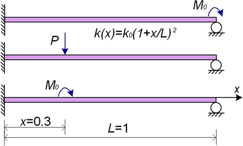
To show the effectiveness of multiple sets of load patterns/static measurements and its influence on the number of elements adopted, different loading cases are considered for this propped cantilever beam: the beam is uniformly partitioned into 25 elements under single load pattern and two load patterns, 50 elements under two load patterns, 100 elements under two load patterns and three load patterns and 200 elements under three load patterns. Three sets of load patterns are used herein: (a) a concentrated moment $M_0=1$ at the right end, (b) a unit concentrated force at $x=0.3$ and (c) a concentrated moment $M_0=1$ at $x=0.3$, as shown in Figure 2. The load pattern is selected randomly for the case with a single load pattern or two load patterns. Displacements under each load pattern are obtained directly from an analytical solution without noise.

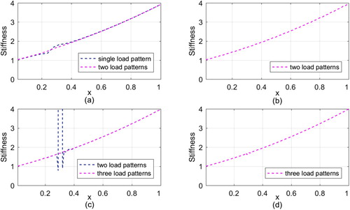
The algorithm in Table 1 is adopted with an initial stiffness being $k^0\left(x\right)=1$. Eventually, the piecewise stiffness can be identified as exhibited in Figure 3. As the number of elements as well as the unknown stiffness parameters increases, the introduction of additional sets of load patterns can help to improve and enhance the identifiability of the algorithm. Limited sets of load patterns and a large number of elements to be identified, such as the case of 25 elements under single load pattern and 100 elements under two load patterns, might lead to the perturbation and deviation in the identification results. In fact, this conclusion not only provides a remedy for possible unidentifiability of the proposed approach, but also is inherent in all inverse identification problems.

Figure 3. Damage identifications in propped cantilever beam: (a) 25 elements under single load pattern and two load patterns, (b) 50 elements under two load patterns, (c) 100 elements under two loads pattern and three load patterns and (d) 200 elements under three load patterns.

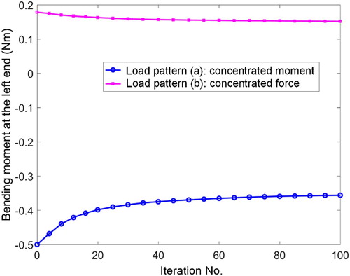
In addition, to show the convergence of the proposed min-CRE approach, the bending moment at the left end of the beam $M(x=0)$ is observed at each iteration step. Detailed results are displayed in Figure 4. It is seen that the bending moment converges only after 20 iterations, verifying the convergence of the two-step substitution algorithm.

Figure 4. Convergence of bending moment at left end of propped cantilever beam.

5.2. Example 2 – a simply supported experimental beam

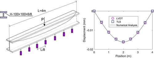
In this example, experimental finite-point measurements are used for stiffness identification to testify the applicability of the modified min-CRE approach. The beam model is taken from the experimental bending test in reference [57]. Parameters of the experimental uniform beam are length $L=4\text{m}$, Young’s modulus $E=206$ GPa and the H-100×100×6/8 section with depth of 100 mm, flange width of 100 mm, web thickness of 6 mm and flange thickness of 8 mm. Only one load case is enforced in the experiment with a concentrated force P = 9.66kN at the middle point of the beam as shown in Figure 5. Experimental displacements attained by the LVDT and the Terrestrial Laser Scanning (TLS) [57] are shown in Figure 5.

Figure 5. Geometry and experimental displacements of simply supported beam.

A noteworthy thing for this problem is that compared to the indeterminate structure in Section 5.1, the structure being analysed herein is statically determinate, which means that the bending moment could be attained without any acknowledgement of the value of stiffness. In spite of this, the two-step iterative algorithm is still needed because the rotations at the nodes are required so as to obtain the full-field displacement based onEquation (23).

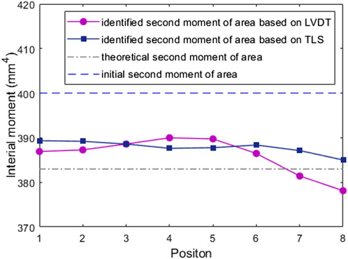
Using these displacement data, the distributive stiffness of the beam can be identified by the modified min-CRE approach and detailed results are presented in Figure 6. The value of the initial uniform second moment of area is set to 400cm⁴. Obviously, the distributive stiffness is well identified with respect to the beam’s theoretical second moment of area 383cm⁴ (Figure 6); the relative errors are less than 3% for both the LVDT data and the TLS data.

Figure 6. Second moment of area identified by modified min-CRE approach comparing to the theoretical second moment of area of simply supported beam.

5.3. Example 3 – a three-span continuous beam

Damage in an equi-spaced three-span continuous and statically indeterminate beam (see Figure 7) is to be identified in this example. The length of each span is $L=2\text{m}$ and the stiffness of the intact beam over the whole beam is $k^0=8.33\times {10}^4\text{N}\cdot {\text{m}}^2$. In this numerical test, measurement points are so distributed that each span is uniformly partitioned into four elements and the specific enumeration of points and elements are also shown in Figure 7.

Figure 7. Geometry, damage location and load cases of three-span continuous beam (D1-damage case 1, D2-damage case 2).

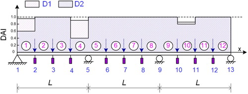
Two damage cases are taken into account, including:

• Small damage case D1: stiffness reduced to 95%, 90% and 85% in elements 1, 4 and 10, respectively; and

• Large damage case D2: stiffness reduced to 60%, 40% and 80% in elements 1, 4 and 10, respectively.

To enhance the identifiability of the algorithm, nine sets of load cases are considered and for each case, a concentrated force is enforced on one of the nodes 2–4, 6–8 and 10–12. Accordingly, nine sets of static displacements at the same nine points are measured. This kind of measurement can often be seen in damage detection of bridges for which a moving truck (or load)is used to generate the multiple load cases.

The simulated displacement data are acquired through finite element computation. A uniform distribution noise is added to the simulated response as (24) $\text{noise}\left(x\right)=uniform\cdot a$(24) where $uniform$ is a number pertains to the uniform distribution and $a$ is the applied noise level. Noise of level 0.1 mm is considered in this example.

For the sake of convenience, the damage index $\text{DAI}$ is introduced to represent the scaled damage in the beam, i.e. (25) $\text{DA}{\text{I}}_i=k_i^{damage}/k_i^0$(25) for the ith element where $k_i^{damage}$ is the damaged stiffness in element i.

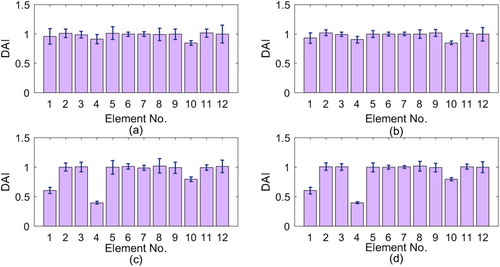
By performing the iterative algorithm in Table 2 with the initial stiffness setting to the stiffness of the intact beam, the min-CRE approach and modified min-CRE approach for damage identification could proceed. To get a better picture for the cases with noise, statistical analysis was performed. Mean values and standard deviations of DAI over 50 Monte Carlo trials are presented in Figure 8. Both large and small damages are well identified in terms of the mean values of the identification results. After additional consideration of the standard deviations, the proposed approach results in better identification of the damage locations and severity of the large damage case than those of the small damage case. Notwithstanding, the identification by the modified min-CRE approach gives better results in terms of the mean values and standard deviations of DAI, verifying the efficiency of the penalty term introduced in Equation (9).

Figure 8. Mean values and standard deviations of DAI with 0.1 mm noise for: (a) small damage case D1 by min-CRE approach, (b) small damage case D1 by modified min-CRE approach, (c) large damage case D2 by min-CRE approach, (d) large damage case D2 by modified min-CRE approach.

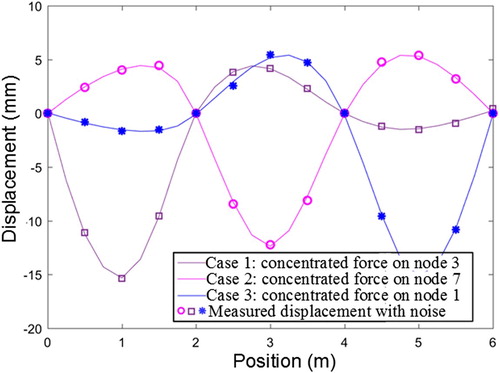
To visualize the convergence of the algorithm for large damage case D2, detailed results on the DAI (see Equation (25)) at each iteration step are given in Figure 9. Obviously, all the quantities converge within 200 iterations and this verifies the convergence of the proposed two-step substitution algorithm. The displacement fields for the large damage case D2 are also rebuilt based on this approach. As can be seen from Figure 10, the ‘uncertainties’ due to the noise in the discrete displacement boundary are much more overcome in these superior rebuilt fields, which results in good identification for the damage.

Figure 9. Convergence of the damage indices of three-span continuous beam under D2.

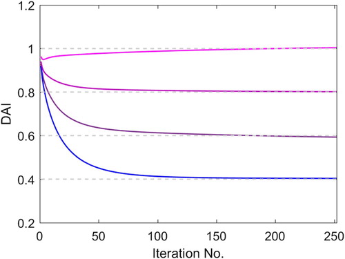
Figure 10. Displacement fields rebuilt by modified min-CRE approach comparing to the displacement boundary.

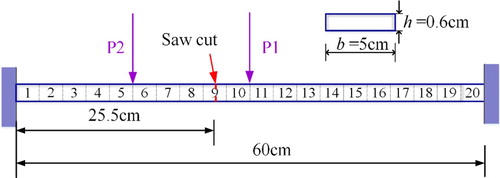
5.4. Example 4 – a cracked experimental beam with two fixed ends

In this example, the modified min-CRE approach was applied to an aluminium beam with two fixed ends [58] as shown in Figure 11. Young’s modulus is E = 70 GPa. A saw cut damage was introduced by cutting two cracks on the top and bottom surface of the intact beam with a depth of quarter of the total thickness of the beam for each crack. Two experimental vertical static load cases, P1 and P2 (Figure 11), were applied using a screw-loading device separately. The static response of the specimen was measured using a micrometre. The finite element model consists of 20 Euler-Bernoulli beam elements with 21 nodes, each with two degrees of freedom (deflection and rotation). The deflection of each node was measured using a micrometre (LVDT) and no information of rotations is available. Based on the FEM computation from reference [58], the saw-cut damage could be simulated using 87.5% reduction of the bending stiffness in the ninth element (see the Reference [58] for details of this experiment).

Figure 11. Geometry and finite element model of the cracked beam with two-fixed ends.

The structural damage identification algorithm in reference [58] was proposed in two stages: the Damage Signature Matching (DSM) technique for detecting the damage locations and furthermore the quadratic optimization programming technique to predict the damage extent. Both static deformation and natural frequencies are required in the damage localization step. To make a comparison with the referenced algorithm, the modified min-CRE approach used in this example is also divided into such two stages: the first stage consists of localizing the most erroneous regions and the second step is the correction of the parameters belonging to these regions.

Figure 12 shows the damage localization results from the min-CRE approach and the referred approach in [58]. The normalized damage index (NDE) could be comprehended as the possibility of damage in each element. When NDE is large, it can be thought that the possibility of damage is very high. As shown in Figure 12(a), the identified results obtained by modified min-CRE approach indicate that elements 8–11 are the most possible damaged elements while the referred approach in [58] clearly detected the damaged element 9. Figure 12 illustrates that the modified min-CRE approach identified the crack, but also suggested damage at other locations close to the crack. This phenomenon may mainly be attributable to the error in modelling as well as the fixed boundary conditions and the deep cracks in the beam may cause the large deflection non-linear effect, which leads to errors in the linear CRE model. Moreover, the CRE identification model did not employ any frequency information compared with the referred approach.

Figure 12. DAI from the min-CRE approach vs. NDE from referred approach [58].

The damage extent was estimated by choosing elements 8–11 and element 9 only as the possible damaged member in the min-CRE approach and the referred approach. This could also be viewed as a regularization procedure so as to achieve a unique solution, which is often used to overcome the ill-posedness of the inverse problem. As shown in Table 3, although obvious errors in the damage extent are still existing in the min-CRE approach, the value of DAI has been much improved by comparing with the results obtained in the damage localization stage without regularization and the DAI in element 9 is closer to the accurate value than the results in reference [58].

Table 3. DAI obtained by modified min-CRE approach comparing with accurate results and results in Reference [58].

		DAI
Method	Possible damaged element	1st load case	2nd load case
Accurate	9	0.125	0.125
Reference	9	0.594	0.580
Min-CRE	8	0.366	0.403
	9	0.290	0.326
	10	0.287	0.315
	11	0.377	0.396

6. Conclusions

Two new approaches based on the minimum constitutive relation error (CRE) principle have been proposed for static damage identification in Bernoulli-Euler beams, i.e. the min-CRE approach for full-field measurements and the modified min-CRE approach for finite-point measurements, respectively. The difference between the two approaches is whether to use additional penalty terms for enforcement of the experimental displacement data or not. A two-step iterative strategy has been established to fulfil the practical implementation and its convergence has been proved. The robustness of these approaches could be guaranteed by applying multiple sets of static measurements. Numerical tests have been carried out to verify these approaches. The sound performance of these proposed approaches in the following aspects have been observed:

1. The approaches are well applicable to both statically determinate and indeterminate beam structures for stiffness/damage identification and bending moment reconstruction;

2. The objective function of these approaches is (separately) convex and large damages could be well identified;

3. The approaches perform well under measurement noise;

4. The approaches converge well in practice.

It should be noted that this study focuses on verifying the static identification efficiency of the min-CRE approach. This process is based on a clear elastic physics model of the structure. In practice, uncertainties from boundary conditions, non-linear effects as well as modelling errors may also be considered. An identification strategy enabling to take into account all the available information and capable to deal with different reliability levels of information using min-CRE approach will be discussed in the future research.

Acknowledgements

The authors are grateful to Professor Hongzhi Zhong of Tsinghua University for the valuable comments for revision.

Disclosure statement

No potential conflict of interest was reported by the authors.

Additional information

Funding

The present investigation was performed under the support of the National Natural Science Foundation of China [grant number 11702336], Guangdong Natural Science Foundation [grant number 2017A030313007] and the MEXT scholarship of Japan. This work was also supported by Ministry of Education, Culture, Sports, Science and Technology.

Appendix

This appendix gives detailed proofs of Theorems 3.1 and 4.1 and clarifies some important theoretical aspects of the proposed approach for Timoshenko beam.

A1. CRE functional for Timoshenko beam

Consider a Timoshenko beam occupying the physical domain $x\in X$. Let u, θ denote the deflection of the mid-point and rotation angle of the mid-surface, respectively, and M, Q the corresponding bending moment and shear force. Material parameters are: flexural stiffness EI and shear stiffness κGA. Support displacements (u,θ) satisfy the homogeneous Dirichlet boundary conditions, and (M,Q) verify homogeneous Neumann boundary conditions. With these notations, the Timoshenko beam model can be described as a combination of the following three parts:

• Kinematic constraints (A1) $\left(u,\theta \right)\in \mathcal{U}$(A1)

• Equilibrium equations

• Find $\left(M,V\right)\in \mathrm{\Im }$ with (A2) $\mathrm{\Im }=\{V=M^{\mathrm{\prime }},V^{\mathrm{\prime }}=q(x),V\text{ and }M\text{ are in equilibrium with }{F}^{ex}\text{ and }{M}^{ex}\}$(A2) with $F^{ex},M^{ex}$ denoting the concentrated loads enforced;

• Constitutive relation (A3) $\begin{array}{c}Q=\kappa GA\left(\theta -u^{\mathrm{\prime }}\right)\\ M=EI{\theta }^{\mathrm{\prime }}\end{array}$(A3) with $\left(EI,\kappa GA\right)\in \mathcal{C}-=\left\{\right(EI,\kappa GA)\in L_2(X):\mathrm{\exists }0<c_0^1<C_0^1,0<c_0^2<C_0^2\text{ such that }{c}_0^1\le EI\le C_0^1,c_0^2\le \kappa GA\le C_0^2\}$ representing a positive and bounded stiffness field.

• Analogous to the case in the Bernoulli-Euler beam, $\mathcal{U}$,$\mathrm{\Im }$,$\mathcal{C}-$ are called the spaces of (kinematically) admissible displacement field, (statically) admissible bending moment field and (constitutively) admissible elastic stiffness field, respectively.

Consider an admissible solution trio $\left\{\left(\overline{u},\overline{\theta }\right),\left(\overline{M},\overline{Q}\right),\left(\overline{E}I,\kappa \overline{G}A\right)\right\}$ which satisfies (A4) $\left(\overline{u},\overline{\theta }\right)\in \mathcal{U},\left(\overline{M},\overline{Q}\right)\in \mathrm{\Im },\left(\overline{E}I,\kappa \overline{G}A\right)\in \mathcal{C}-$(A4) To measure the distance of the admissible solution trio to the exact solution trio in energy product, an error in constitutive relation for the Timoshenko beam is introduced (A5) $e_{CRE}=\frac{1}{2}{\int }_X\left\{\frac{{(\overline{M}-\overline{E}I{\overline{\theta }}^{\mathrm{\prime }})}^2}{\overline{E}I}+\frac{{(\overline{Q}-\kappa \overline{G}A(\overline{\theta }-{\overline{u}}^{\mathrm{\prime }}\left)\right)}^2}{\kappa \overline{G}A}\right\}\text{d}x$(A5)

A2. Proof of Theorem 3.1

(a), (b) and (c) are obvious from reference [23].

(d) Denote the minimizer by $(M,k)$, which satisfies the following two conditions, (A6) ${\int }_X\frac{M^2}{k^2}\delta \overline{k}\text{d}x={\int }_X{\left(w^{\mathrm{\prime \prime }}\right)}^2\delta \overline{k}\text{d}x,\mathrm{\forall }\delta \overline{k}\in {\mathcal{C}}_0,$(A6) and (A7) ${\int }_X\frac{M}{k}\delta \overline{M}\text{d}x={\int }_X{w}^{\mathrm{\prime \prime }}\delta \overline{M}\text{d}x,\mathrm{\forall }\delta \overline{M}\in {\mathrm{\Im }}_0$(A7) Then, contradiction is utilized to verify (A8) $\mu (x\in X:w^{\mathrm{\prime \prime }}(x)=0)=0\Rightarrow \mu (x\in X:M(x)=0)=0$(A8) Assume that there exists a subset $X_{pp}\subseteq X$ with $\mu \left(X_{pp}\right)>0$ such that $M\left(x\right)=0$ on $X_{pp}$. Trivially, substitution of $\delta \overline{k}=\left\{\begin{array}{l}c,x\in X_{pp}\\ 0,x\in X\mathrm{\setminus }{X}_{pp}\end{array}\right.,c=\frac{1}{2}(C_0-c_0)>0$ into Equation (A6) yields (A9) ${\int }_{X_{pp}}c{\left(w^{\mathrm{\prime \prime }}\right)}^2\text{d}x=0$(A9) which contradicts with the condition $\mu \left(w^{\mathrm{\prime \prime }}\right(x)=0,x\in X)=0$.

Next, let ${\delta }_{\overline{M}}^{2}F$ and ${\delta }_{\overline{k}}^{2}F$ denote the second order variations on $F(\cdot ,\cdot )$ for $\overline{M}$ and $\overline{k}$, respectively. Simple manipulations lead to (A10) $\begin{array}{l}{\delta }_{\overline{M}}^{2}F={\int }_X\frac{{\left(\delta \overline{M}\right)}^2}{\overline{k}}\text{d}x\ge \frac{1}{C_0}{\int }_X{\left(\delta \overline{M}\right)}^2\text{d}x>0,\\ {\delta }_{\overline{k}}^{2}F={\int }_X\frac{{\overline{M}}^2}{{\overline{k}}^3}{\left(\delta \overline{k}\right)}^2\text{d}x\ge \frac{1}{C_0^3}{\int }_X{\overline{M}}^2{\left(\delta \overline{k}\right)}^2\text{d}x>0\end{array}$(A10) for ${\int }_X{\left(\delta \overline{M}\right)}^{2}dx>0$, ${\int }_X{\left(\delta \overline{k}\right)}^{2}dx>0$ and $\overline{M}\in {\mathrm{\Im }}^{\ast }$, indicating the separately strict convexity on${\mathrm{\Im }}^{\ast }\times \mathcal{C}$.

Remark A1:

From Equation (A7), it is found that (A11) ${\int }_X\frac{\overline{M}}{\overline{k}}\delta \overline{M}\text{d}x={\int }_X{w}^{\mathrm{\prime \prime }}\delta \overline{M}\text{d}x={\sum }_p({\theta }_p\delta \overline{M}{|}_p+w_p\left(\delta \overline{M}{)}^{\mathrm{\prime }}{|}_p\right)$(A11) where the subscript p indicates the prescribed displacement boundary condition. Obviously, Equation (A11) embodies the minimum complementary energy principle (A12) $M\left(\overline{k}\right)=\arg \underset{\overline{M}\in \mathrm{\Im }}{min}\left\{\frac{1}{2}{\int }_X\frac{{\overline{M}}^2}{\overline{k}}\text{d}x-{\sum }_p({\theta }_p\overline{M}{|}_p+w_p\left(\overline{M}{)}^{\mathrm{\prime }}{|}_p\right)\right\}$(A12) and corresponds to a unique mapping $d:\mathcal{C}\to \mathcal{U}$ such that (A13) ${\int }_X\overline{k}{\left(\text{d}\left(\overline{k}\right)\right)}^{\mathrm{\prime \prime }}{v}^{\mathrm{\prime \prime }}\text{d}x={\int }_{X}q\left(x\right)v\text{d}x+\sum \left(F^{ex}v\right(x^{ex})+M^{ex}{v}^{\mathrm{\prime }}(x^{ex}\left)\right),\mathrm{\forall }v\in {\mathcal{U}}_0$(A13) and $M\left(\overline{k}\right)=\overline{k}(d\left(\overline{k}\right){)}^{\mathrm{\prime \prime }}$. With these notations, the minimization problem (7) can become (A14) $\underset{\overline{M}\in \mathrm{\Im },\overline{k}\in \mathcal{C}}{min}F(\overline{M},\overline{k})=\underset{\overline{k}\in \mathcal{C}}{min}\frac{1}{2}{\int }_X\frac{{\left(M\right(\overline{k})-\overline{k}{w}^{\mathrm{\prime \prime }})}^2}{\overline{k}}\text{d}x=\underset{\overline{k}\in \mathcal{C}}{min}\frac{1}{2}{\int }_X\overline{k}{|{\left(d\right(\overline{k})-w)}^{\mathrm{\prime \prime }}|}^2\text{d}x$(A14) which is a common variational form for inverse identification and its well-posedness has been investigated in a variety of work (see [59–61] for instance). As indicated in the work, problem (39) as well as problem (7) will have a unique minimizer if $\underset{x\in X}{inf}|w^{\mathrm{\prime \prime }}|>0$ and $\overline{k}$ is prescribed along the inflow portion of the boundary [62]. It is noted that $\underset{x\in X}{inf}|w^{\mathrm{\prime \prime }}|>0$ is a stronger version of the deforming condition$\mu (x\in X:w^{\mathrm{\prime \prime }}(x)=0)=0$.

For proof of Theorem 4.1, a lemma is introduced first.

Lemma A1:

Let $f:H\to \mathsf{R}$ be a continuous and strictly convex function and $u\in H$ be its unique minimizer, where $H$ is a compact Banach space with norm $||\cdot ||$. Then, for an arbitrary sequence $\{u_n{\}}_{n=0}^{\mathrm{\infty }}\in H$ satisfying $\underset{n\to \mathrm{\infty }}{lim}f\left(u_n\right)=f\left(u\right)$, one has (A15) $\underset{n\to \mathrm{\infty }}{lim}||u_n-u||=0$(A15)

Proof:

This is obvious by contradiction. Assume that $||u_n-u||$ does not converge to zero; that is, there exists a positive constant $\epsilon$ such that for an arbitrary positive integer $N>0$, there is $m\ge N$ with $||u_m-u||>\epsilon$.

Note that $H_{\epsilon }=\{v\in H:||v-u||\ge \epsilon \}$ is a compact subspace of $H$ and therefore, $f$ is also continuous and strictly convex on $H_{\epsilon }$, implying that there is $u_{\epsilon }\in H_{\epsilon }$ such that (A16) $u_{\epsilon }=\arg \underset{v\in H_{\epsilon }}{min}f\left(v\right)$(A16) By the strict convexity, one has $f\left(u_{\epsilon }\right)>f\left(u\right)$ and hence $f\left(u_m\right)\ge f\left(u_{\epsilon }\right)>f\left(u\right)$, contradicting with $\underset{n\to \mathrm{\infty }}{lim}f\left(u_n\right)=f\left(u\right)$.

A3. Proof of Theorem 4.1

From the two-step substitution algorithm in Table 1, one has for $(M^0,k^0)\in {\mathrm{\Im }}^{\ast }\times {\mathcal{C}}_h$ and the integer $n\ge 0$ (A17) $\begin{array}{l}{k}^{n+1}=\arg \underset{\overline{k}\in {\mathcal{C}}_h}{min}F(M^n,\overline{k}),\\ M^{n+1}=\arg \underset{\overline{M}\in {\mathrm{\Im }}^{\ast }}{min}F(\overline{M},k^{n+1}).\end{array}$(A17) Then, define a sequence $\{F_n{\}}_{n=0}^{\mathrm{\infty }}$ as (A18) $F_{2m}=F(M^m,k^m),F_{2m+1}=F(M^m,k^{m+1}),m\in \mathbb{N}$(A18) and by considering Equation (A17), one has (A19) $F_{2m}\ge F_{2m+1}\ge F_{2m+2}$(A19) Along with Theorem 3.1(a), it is seen that $F_n\ge 0,n=0,1,\dots$ and thus, it is deduced that $\{F_n{\}}_{n=0}^{\mathrm{\infty }}$ is a decreasing and bounded (from below) sequence, meaning that $\{F_n{\}}_{n=0}^{\mathrm{\infty }}$ is a Cauchy sequence. Furthermore, uniqueness of the minimizer must require $(M_h,k_h)\in {\mathrm{\Im }}^{\ast }\times {\mathcal{C}}_h$ and by Theorem 3.1(d), $F(\cdot ,\cdot )$ is separately strictly-convex on ${\mathrm{\Im }}^{\ast }\times {\mathcal{C}}_h$. Thus, on considering Lemma A1, one has (A20) $\begin{array}{l}{F}_{2m+1}-F_{2m}\to 0\Rightarrow ||k^{m+1}-k^m|{|}_{L^2}\to 0,\\ F_{2m+2}-F_{2m+1}\to 0\Rightarrow ||M^{m+1}-M^m|{|}_{L^2}\to 0.\end{array}$(A20) By further exploiting the information in Equation (A17), one has (A21) ${\mathrm{\nabla }}_{\overline{k}}F(M^n,k^{n+1})\cdot \delta \overline{k}:={\int }_X[-(\frac{M^n}{k^{n+1}}{)}^2+(w^{\mathrm{\prime \prime }}{)}^2]\delta \overline{k}dx=0$(A21) and (A22) ${\mathrm{\nabla }}_{\overline{M}}F(M^{n+1},k^{n+1})\cdot \delta \overline{M}:={\int }_X(\frac{M^{n+1}}{k^{n+1}}-w^{\mathrm{\prime \prime }})\delta \overline{M}dx=0$(A22) By continuity, it is inferred from Equations (A21) and (A20) that (A23) ${\mathrm{\nabla }}_{\overline{k}}F(M^{n+1},k^{n+1})\cdot \delta \overline{k}\to {\mathrm{\nabla }}_{\overline{k}}F(M^n,k^{n+1})\cdot \delta \overline{k}=0,\text{ as }n\to \mathrm{\infty }$(A23) Next, it is concluded from Equations (A22) and (A23) that (A24) $\underset{n\to \mathrm{\infty }}{lim}\left(\begin{array}{l}{\mathrm{\nabla }}_{\overline{M}}F(M^n,k^n)\cdot \delta \overline{M}\\ {\mathrm{\nabla }}_{\overline{k}}F(M^n,k^n)\cdot \delta \overline{k}\end{array}\right)=\left(\begin{array}{l}0\\ 0\end{array}\right)$(A24) By Taylor expansion [63] at the minimizer $(M_h,k_h)$, one can have (A25) $\begin{array}{l}\left(\begin{array}{l}{\mathrm{\nabla }}_{\overline{M}}F(M^n,k^n)\cdot \delta \overline{M}\\ {\mathrm{\nabla }}_{\overline{k}}F(M^n,k^n)\cdot \delta \overline{k}\end{array}\right)=\left(\begin{array}{l}{\mathrm{\nabla }}_{\overline{M}}F(M_h,k_h)\cdot \delta \overline{M}\\ {\mathrm{\nabla }}_{\overline{k}}F(M_h,k_h)\cdot \delta \overline{k}\end{array}\right)+{\left(\begin{array}{l}{M}^n-M_h\\ k^n-k_h\end{array}\right)}^T\cdot J(M_{\xi },k_{\varsigma })\cdot \left(\begin{array}{l}\delta \overline{M}\\ \delta \overline{k}\end{array}\right)\\ ={\left(\begin{array}{l}{M}^n-M_h\\ k^n-k_h\end{array}\right)}^T\cdot J(M_{\xi },k_{\varsigma })\cdot \left(\begin{array}{l}\delta \overline{M}\\ \delta \overline{k}\end{array}\right)\end{array}$(A25) where $(M_{\xi },k_{\varsigma })$ is the linear interpolation of between $(M^n,k^n)$ and $(M_h,k_h)$, $J(M_{\xi },k_{\varsigma })$ is the second order Hessian matrix of $F(\cdot ,\cdot )$ at $(M_{\xi },k_{\varsigma })$. Trivially, inserting $\delta \overline{M}=M^n-M_h$ and $\delta \overline{k}=k^n-k_h$ into Equation (A25) and noticing the fact that $J(M_{\xi },k_{\varsigma })$ is positive definite due to the strict convexity of $F(\cdot ,\cdot )$ in the vicinity of $(M_h,k_h)$, it eventually follows from Equations (A24) and (A25) that (A26) $\underset{n\to \mathrm{\infty }}{lim}||M^n-M_h|{|}_{L^2}=0,\underset{n\to \mathrm{\infty }}{lim}||k^n-k_h|{|}_{L^2}=0$(A26)

References

- Fan W, Qiao P. Vibration-based damage identification methods: a review and comparative study. Struct Health Monit. 2011;10:83–111. doi: 10.1177/1475921710365419
- Di Paola M, Bilello C. An integral equation for damage identification of Euler-Bernoulli beams under static loads. J Eng Mech. 2004;130:225–234. doi: 10.1061/(ASCE)0733-9399(2004)130:2(225)
- Abdo MA-B. Parametric study of using only static response in structural damage detection. Eng Struct. 2012;34:124–131. doi: 10.1016/j.engstruct.2011.09.027
- Huynh D, He J, Tran D. Damage location vector: a non-destructive structural damage detection technique. Comput Struct. 2005;83:2353–2367. doi: 10.1016/j.compstruc.2005.03.029
- Sung S, Jung H, Jung H. Damage detection for beam-like structures using the normalized curvature of a uniform load surface. J Sound Vib. 2013;332:1501–1519. doi: 10.1016/j.jsv.2012.11.016
- Abdo M-B, Hori M. A numerical study of structural damage detection using changes in the rotation of mode shapes. J Sound Vib. 2002;251:227–239. doi: 10.1006/jsvi.2001.3989
- Cornwell P, Doebling SW, Farrar CR. Application of the strain energy damage detection method to plate-like structures. J Sound Vib. 1999;224:359–374. doi: 10.1006/jsvi.1999.2163
- Debruyne S, Vandepitte D, Moens D. Identification of design parameter variability of honeycomb sandwich beams from a study of limited available experimental dynamic structural response data. Comput Struct. 2015;146:197–213. doi: 10.1016/j.compstruc.2013.09.004
- Greco A, Pau A. Damage identification in Euler frames. Comput Struct. 2012;92–93:328–336. doi: 10.1016/j.compstruc.2011.10.007
- Pandey A, Biswas M. Damage detection in structures using changes in flexibility. J Sound Vib. 1994;169:3–17. doi: 10.1006/jsvi.1994.1002
- Pandey A, Biswas M, Samman M. Damage detection from changes in curvature mode shapes. J Sound Vib. 1991;145:321–332. doi: 10.1016/0022-460X(91)90595-B
- Salawu O. Detection of structural damage through changes in frequency: a review. Eng Struct. 1997;19:718–723. doi: 10.1016/S0141-0296(96)00149-6
- Banan MR, Banan MR, Hjelmstad K. Parameter estimation of structures from static response. I. computational aspects. J Struct Eng. 1994;120:3243–3258. doi: 10.1061/(ASCE)0733-9445(1994)120:11(3243)
- Banan MR, Banan MR, Hjelmstad KD. Parameter Estimation of structures from static response. II: numerical simulation studies. J Struct Eng. 1994;120:3259–3283. doi: 10.1061/(ASCE)0733-9445(1994)120:11(3259)
- Viola E, Bocchini P. Non-destructive parametric system identification and damage detection in truss structures by static tests. Struct Infrastruct Eng. 2013;9:384–402. doi: 10.1080/15732479.2011.560164
- Ghrib F, Li L, Wilbur P. Damage identification of Euler–Bernoulli beams using static responses. J Eng Mech. 2012;138:405–415. doi: 10.1061/(ASCE)EM.1943-7889.0000345
- Avril S, Pierron F. General framework for the identification of constitutive parameters from full-field measurements in linear elasticity. Int J Solids Struct. 2007;44:4978–5002. doi: 10.1016/j.ijsolstr.2006.12.018
- Yang Q, Sun B. Structural damage localization and quantification using static test data. Struct Health Monitor. 2011;10:381–389. doi: 10.1177/1475921710379517
- Rezaiee-Pajand M, Kazemiyan MS, Aftabi SA. Static damage identification of 3D and 2D frames. Mech Based Des Struct Mach. 2014;42:70–96. doi: 10.1080/15397734.2013.830534
- Caddemi S, Greco A. The influence of instrumental errors on the static identification of damage parameters for elastic beams. Comput Struct. 2006;84:1696–1708. doi: 10.1016/j.compstruc.2006.03.010
- Bakhtiari-Nejad F, Rahai A, Esfandiari A. A structural damage detection method using static noisy data. Eng Struct. 2005;27:1784–1793. doi: 10.1016/j.engstruct.2005.04.019
- Ladevèze P, Chouaki A. Application of a posteriori error estimation for structural model updating. Inverse Probl. 1999;15:49–58. doi: 10.1088/0266-5611/15/1/009
- Geymonat G, Pagano S. Identification of mechanical properties by displacement field measurement: A variational approach. Meccanica. 2003;38:535–545. doi: 10.1023/A:1024766911435
- Florentin E, Lubineau G. Identification of the parameters of an elastic material model using the constitutive equation gap method. Comput Mech. 2010;46:521–531. doi: 10.1007/s00466-010-0496-y
- Florentin E, Lubineau G. Using constitutive equation gap method for identification of elastic material parameters: technical insights and illustrations. Int J Interact Des Manuf. 2011;5:227–234. doi: 10.1007/s12008-011-0129-5
- Lubineau G. A goal-oriented field measurement filtering technique for the identification of material model parameters. Comput Mech. 2009;44:591–603. doi: 10.1007/s00466-009-0392-5
- Moussawi A, Lubineau G, Florentin E, Blaysat B. The constitutive compatibility method for identification of material parameters based on full-field measurements. Comput Methods Appl Mech Eng. 2013;265:1–14. doi: 10.1016/j.cma.2013.06.003
- Maunder E, de Almeida JM, Ramsay A. A general formulation of equilibrium macro-elements with control of spurious kinematic modes: the exorcism of an old curse. Int J Numer Method Eng. 1996;39:3175–3194. doi: 10.1002/(SICI)1097-0207(19960930)39:18<3175::AID-NME978>3.0.CO;2-3
- Wang L, Zhong H. A traction-based equilibrium finite element free from spurious kinematic modes for linear elasticity problems. Int J Numer Methods Eng. 2014;99:763–788. doi: 10.1002/nme.4701
- Sedaghati R, Suleman A. Force method revisited. AIAA J. 2003;41:957–966. doi: 10.2514/2.2033
- Bonnet M, Constantinescu A. Inverse problems in elasticity. Inverse Probl. 2005;21:R1–R50. doi: 10.1088/0266-5611/21/2/R01
- Celebi M. GPS in dynamic monitoring of long-period structures. Soil Dyn Earthq Eng. 2000;20:477–483. doi: 10.1016/S0267-7261(00)00094-4
- Nickitopoulou A, Protopsalti K, Stiros S. Monitoring dynamic and quasi-static deformations of large flexible engineering structures with GPS: accuracy, limitations and promises. Eng Struct. 2006;28:1471–1482. doi: 10.1016/j.engstruct.2006.02.001
- Chen F, Brown GM, Song MM. Overview of three-dimensional shape measurement using optical methods. Opt Eng. 2000;39:10–22. doi: 10.1117/1.602438
- Ekstrom MP. Digital image processing techniques. New York (NY): Academic Press; 2012.
- Choi SW, Kim BR, Lee HM, Kim Y, Park HS. A deformed shape monitoring model for building structures based on a 2D laser scanner. Sensors (Basel). 2013;13:6746–6758. doi: 10.3390/s130506746
- Park HS, Lee HM, Adeli H, Lee I. A new approach for health monitoring of structures: Terrestrial laser scanning. Comput-Aided Civ Infrastruct Eng. 2007;22:19–30. doi: 10.1111/j.1467-8667.2006.00466.x
- Nassif HH, Gindy M, Davis J. Comparison of laser Doppler vibrometer with contact sensors for monitoring bridge deflection and vibration. NDT E Int. 2005;38:213–218. doi: 10.1016/j.ndteint.2004.06.012
- Hild F, Roux S. Digital image correlation: from displacement measurement to identification of elastic properties – a review. Strain. 2006;42:69–80. doi: 10.1111/j.1475-1305.2006.00258.x
- Jiang R, Jáuregui DV, White KR. Close-range photogrammetry applications in bridge measurement: literature review. Measurement ( Mahwah N J). 2008;41:823–834.
- Patsias S, Staszewski WJ. Damage detection using optical measurements and Wavelets. Struct Health Monit. 2002;1:5–22. doi: 10.1177/147592170200100102
- Ji YF, Chang CC. Nontarget image-based technique for small cable vibration measurement. J Bridge Eng. 2008;13:34–42. doi: 10.1061/(ASCE)1084-0702(2008)13:1(34)
- Morlier J, Michon G. Virtual Vibration measurement using KLT motion tracking algorithm. J Dyn Syst Meas Control. 2010;132:011003. doi: 10.1115/1.4000070
- Park J-W, Lee J-J, Jung H-J, et al. Vision-based displacement measurement method for high-rise building structures using partitioning approach. NDT E Int. 2010;43:642–647. doi: 10.1016/j.ndteint.2010.06.009
- Fu G, Moosa AG. An optical approach to structural displacement measurement and its application. J Eng Mech. 2002;128:511–520. doi: 10.1061/(ASCE)0733-9399(2002)128:5(511)
- Choi H-S, Cheung J-H, Kim S-H, et al. Structural dynamic displacement vision system using digital image processing. NDT E Int. 2011;44:597–608. doi: 10.1016/j.ndteint.2011.06.003
- Jurjo DLBR, Magluta C, Roitman N, et al. Experimental methodology for the dynamic analysis of slender structures based on digital image processing techniques. Mech Syst Signal Process. 2010;24:1369–1382. doi: 10.1016/j.ymssp.2009.12.006
- Kim S-W, Kim N-S. Multi-point displacement response measurement of Civil Infrastructures using digital image processing. Procedia Eng. 2011;14:195–203. doi: 10.1016/j.proeng.2011.07.023
- Lee JJ, Shinozuka M. A vision-based system for remote sensing of bridge displacement. NDT E Int. 2006;39:425–431. doi: 10.1016/j.ndteint.2005.12.003
- Nakamura S. GPS measurement of wind-induced suspension bridge girder displacements. J Struct Eng-Asce. 2000;126:1413–1419. doi: 10.1061/(ASCE)0733-9445(2000)126:12(1413)
- Park SW, Park HS, Kim JH, et al. 3D displacement measurement model for health monitoring of structures using a motion capture system. Measurement (Mahwah NJ). 2015;59:352–362. doi: 10.1016/j.measurement.2014.09.063
- Wahbeh AM, Caffrey JP, Masri SF. A vision-based approach for the direct measurement of displacements in vibrating systems. Smart Mater Struct. 2003;12:785–794. doi: 10.1088/0964-1726/12/5/016
- Olaszek P. Investigation of the dynamic characteristic of bridge structures using a computer vision method. Measurement ( Mahwah NJ). 1999;25:227–236. Epub 236.
- Ladeveze P, Leguillon D. Error estimate procedure in the finite element method and applications. SIAM J Numer Anal. 1983;20:485–509. doi: 10.1137/0720033
- Charbonnel P-E, Ladevèze P, Louf F, et al. A robust CRE-based approach for model updating using in situ measurements. Comput Struct. 2013;129:63–73. doi: 10.1016/j.compstruc.2013.08.002
- Widlak T, Scherzer O. Stability in the linearized problem of quantitative elastography. Inverse Probl. 2015;31(3):035005. doi: 10.1088/0266-5611/31/3/035005
- Lee HM, Park HS. Gage-Free Stress Estimation of a beam-like structure based on Terrestrial laser scanning. Comput-Aided Civ Infrastruct Eng. 2011;26:647–658. doi: 10.1111/j.1467-8667.2011.00723.x
- Wang X, Hu N, Fukunaga H, et al. Structural damage identification using static test data and changes in frequencies. Eng Struct. 2001;23:610–621. doi: 10.1016/S0141-0296(00)00086-9
- Knowles I. Uniqueness for an elliptic inverse problem. SIAM J Appl Math. 1999;59:1356–1370. doi: 10.1137/S0036139997327782
- Knowles I Parameter identification for elliptic problems. J Comput Appl Math. 2001;131:175–194. doi: 10.1016/S0377-0427(00)00275-2
- Kohn RV, Lowe BD. A variational method for parameter identification. RAIRO-Modelisation Mathématique et Analyse Numérique. 1988;22:119–158.
- Richter GR. An inverse problem for the steady state diffusion equation. SIAM J Appl Math. 1981;41:210–221. doi: 10.1137/0141016
- Kolda TG, Lewis RM, Torczon V. Optimization by direct search: New perspectives on some classical and modern methods. SIAM Rev. 2003;45:385–482. doi: 10.1137/S003614450242889