A new approach to speed up the conjugate gradient method by applying the complex variable differentiation method

ABSTRACT

This study represents a novel approach to speed up the solution of nonlinear inverse heat conduction problems (IHCPs) by the implementation of the complex variable differentiation method (CVDM). A difficulty appeared in the solution of nonlinear problems is the great amount of computational time. To handle this problem, a new scheme is introduced to improve the conjugate gradient method (CGM). The main contribution in the improvement of conventional CGM is the simultaneous solution of direct and sensitivity problems by applying the complex variable method. The derivation of sensitivity problem by utilizing the analytic derivative is difficult or impossible, since the direct problem is complicated mathematically in many cases. By this approach, the analytic derivation of sensitivity problem is circumvented, while the Jacobian matrix components are obtained accompanied by the solution of the direct problem. Therefore, the developed scheme results in the reduction of mathematical manipulations. Due to the high nonlinearity of moving boundary inverse problems, the ablation problem is considered as the benchmark to examine the accuracy and effectiveness of the proposed scheme. The simulated results illustrate that the developed scheme has the potential to significantly reducing of the computational expenses while maintaining the quality of numerical solution.

KEYWORDS:

• Modified conjugate gradient method
• complex variable differentiation method
• sensitivity problem
• ablation problem
• nonlinear inverse problems

SUBJECT CLASSIFICATION CODES:

• 65B99
• 35K05
• 35K55
• 30A99

1. Nomenclature

$c_p$	=	specific heat, J kg−1 K−1
$\mathbf{d}$	=	direction of decent vector
$f$	=	function
$F$	=	objective function
$H$	=	ablation heat, J kg−1
$i$	=	imaginary unit
$I$	=	number of spatial intervals
$\mathbf{J}$	=	sensitivity matrix
$k$	=	thermal conductivity, W m−1 K−1
$L$	=	slab length, m
$M$	=	number of unknowns
$N$	=	number of measured temperatures
$P$	=	number of time intervals
$q$	=	heat flux, W m−2
$Q$	=	dimensionless heat flux
$S$	=	dimensionless ablating surface position
$t$	=	time, s
$T$	=	temperature, K
$TS$	=	time step
$x$	=	Cartesian coordinate, m
$X$	=	dimensionless length
$Y$	=	dimensionless measured temperature
$Z$	=	transformed front position

Greek symbols

$\theta$	=	dimensionless temperature
$\tau$	=	dimensionless time
$\nu$	=	dimensionless heat of ablation
$\alpha$	=	thermal diffusivity, m2 s−1
$\sigma$	=	standard deviation
$\omega$	=	random variable
$\gamma$	=	conjugation coefficient
$\beta$	=	search step size

Superscripts

$0$	=	initial at $t=0$
$k$	=	iteration number
$T$	=	transpose of matrix
$TS$	=	time step

Superscripts

$a$	=	ablative
$c$	=	convective
$com$	=	computed value
$exa$	=	exact value
$f$	=	final time
$i$	=	initial value
$s$	=	start time
$ab$	=	ablation

1. Introduction

The inverse heat conduction problems (IHCPs) rely on the prediction of unknown quantities which are practically difficult or impossible to measure in the wide range of thermal engineering processes. The unknowns appeared in the inverse analysis of physical problems include the applied boundary conditions, thermal properties of materials or recently optimal geometries of thermal devices [1–6]. Following the developments of numerical tools, numerous techniques were proposed by researchers in the last decades [7,8]. Among the suggested schemes, the conjugate gradient method (CGM) was widely used in the lots of former studies due to its simplicity and robustness [7]. However, a few number of investigations concentrated on the improvement of the CGM in the conventional form [9]. Besides the advantages of the standard CGM, the inherent iterative procedure of this method is highly time-consuming, particularly in the solution of nonlinear problems. Moreover, obtaining and solving the mathematical governing equations of sensitivity problem are a cumbersome task in many inverse analyses. To overcome these drawbacks and to speed up the standard CGM, several methods such as the precise calculation of sensitivity coefficients and the application of relaxation factor were proposed [9,10].

With regard to the importance of inverse analysis in the vast engineering applications, the improvement of available inverse methods draws considerable attentions to this category of engineering science [11–14]. Just recently, the complex variable differentiation method (CVDM) was utilized to compute the sensitivity coefficients in a number of inverse heat transfer problems [9,10,15–20]. Implementing aforementioned approach in calculating the sensitivity coefficients was used to attenuate the effects of truncation error caused by the numerical discretization schemes such as finite element method (FEM) and boundary element method (BEM) [21–23]. Therefore, the values of sensitivity are computed in a more precise form.

Current study introduces a novel approach in the improvement of the conventional CGM to fasten the computational procedure while the quality of the solution is maintained, particularly for nonlinear problems. The main contribution in the improvement of CGM is achieved by the simultaneous solution of direct and sensitivity problems applying the CVDM. The iterative procedure of the CGM includes the solution of direct and sensitivity problems in two distinct steps. In general, increasing the number of stages in the numerical algorithm enhances the mathematical complexity and computational time expenses in the solution process. A further difficulty comes from the analytic determination of the sensitivity coefficients by differentiating the direct problem which is not feasible in all circumstances. The treatment of CGM is accomplished by merging the solution of direct and sensitivity problems in conjugation with the exact computation of sensitivity coefficients using a complex differentiation method. The previous works only concentrated on using the CVDM to calculate the sensitivity with more precision [9,16,18–20, 24]. In addition, solely pure heat conduction problems were investigated [9]. To illustrate the effectiveness of the developed scheme in the reduction of required mathematical manipulations and improvement of numerical efficiency, a high nonlinear moving boundary problem is chosen. In the present research, the ablation is assumed to be as benchmark. The ablation belongs to the class of moving boundary problems that happens in many industrial applications, such as thermal design of heat shields and reverberatory smelting furnaces [5,25–27]. In accordance with the high nonlinearity of moving boundary problems, their mathematical processing requires high computational expenses. Due to severe conditions through the medium in which the ablation process occurs, the presented modified CGM can provide a suitable numerical tool to estimate the unknown parameters such as applied heat flux at the end surfaces of ablating material. It is shown by the implementation of the developed scheme the convergence rate of numerical solution is boosted considerably while the solution quality is maintained.

This paper includes four main sections. The complex differentiation method and its application in the modification of the standard CGM are described in Sections 2 and 3, respectively. Section 4 presents the computational algorithm of MCGM, whereas the moving boundary ablation problem is solved as benchmark by the proposed inverse scheme in Section 5. The conclusions are drawn in the last section.

2. Complex variable differentiation method

Lack of an analytic solution for a wide range of partial differential equations encouraged many researchers to utilize the discretization scheme to obtain the approximate solution of this class of mathematical equations [28–30]. Among the available schemes, the finite difference formulas were extensively used to estimate the values of derivatives. These formulas are based on truncating the Taylor series expanded about a point $x$. A common technique to estimate the first derivative is given as follows [29]: (1) $\frac{\mathrm{\partial }f\left(x\right)}{\mathrm{\partial }x}\approx \frac{f(x+\mathrm{\Delta }x)-f\left(x\right)}{\mathrm{\Delta }x},\left(1\right)$(1) where $\mathrm{\Delta }x$ is the increment in $x$ direction. This approximation is an $O\left(\mathrm{\Delta }x\right)$ that estimates the first derivative of $f\left(x\right)$. By using the finite difference method (FDM) to estimate the sensitivities, a difficulty arises from the truncation error in the numerical approximation. In order to overcome this problem, the CVDM pioneered by Lyness and Moler [23] is suggested. To clarify the concept of CVDM, let us consider a real function $f\left(x\right)$. By substituting $x+ih$ with $x$, and employing the Taylor series expansion about $h$ we have (2) $f(x+ih)=f\left(x\right)+ih{f}^{\mathrm{\prime }}\left(x\right)-\frac{h^2}{2}{f}^{\mathrm{\prime \prime }}\left(x\right)+\cdots .\left(2\right)$(2)

By rearranging Equation (2), the CVDM gives the estimation of first derivative of $f\left(x\right)$ for a very small discrete of $h$ (usually $h={10}^{-20}$) as follows [22]: (3) $\frac{\mathrm{\partial }f\left(x\right)}{\mathrm{\partial }x}\approx \frac{\mathrm{Im}\left[f(x+ih)\right]}{h}.\left(3\right)$(3) The proposed estimation is an $O\left(h^2\right)$. It is obvious that the aforementioned numerical technique in computing the first derivative is considerably more accurate than standard FDM. Since, the first derivative is applied in the computation of Jacobian matrix component, implementing the CVDM to calculate the sensitivity coefficients improves the efficiency of analysis.

3. Modified conjugate gradient method

The powerful and straightforward nature of the CGM results in its vast applications in solving the linear and nonlinear inverse problems [7]. The standard CGM is an iterative gradient-based approach based on the minimization of least square objective function described as (4) $F=(\mathbf{Y}-\mathbf{T}{)}^{\mathrm{T}}(\mathbf{Y}-\mathbf{T}),\left(4\right)$(4) where $\mathbf{Y}$ and $\mathbf{T}$ define the measured and computed temperatures, respectively. In the iterative procedure of the CGM, at each iteration a suitable step size $\beta$ is taken along a direction of descent $\text{d}$ in order to minimize the above norm $F$, so that [7] (5) ${\mathbf{P}}^{k+1}={\mathbf{P}}^k-{\beta }^k{\mathbf{d}}^k,\left(5\right)$(5) where the superscript $k$ is the iteration number. The direction of descent is a conjugation of gradient direction$\mathrm{\nabla }F$ and the direction of descent in the previous iteration ${\mathbf{d}}^{k-1}$. It is given as [7] (6) ${\mathbf{d}}^k=\mathrm{\nabla }{F}^k+\gamma {\mathbf{d}}^{k-1},\left(6\right)$(6) where $\gamma$ is the conjugation coefficient given by [7] (7) ${\gamma }^k=\frac{\mathrm{\nabla }F\left({\mathbf{P}}^k\right)\mathrm{\nabla }{F}^{\mathrm{T}}\left({\mathbf{P}}^k\right)}{\mathrm{\nabla }F\left({\mathbf{P}}^{k-1}\right)\mathrm{\nabla }{F}^{\mathrm{T}}\left({\mathbf{P}}^{k-1}\right)}\text{with}{\gamma }^0=0.\left(7\right)$(7) The gradient direction vector is determined as [7] (8) $\mathrm{\nabla }F\left({\mathbf{P}}^k\right)=-2({\mathbf{J}}^k{)}^{\mathrm{T}}\left[\mathbf{Y}-\mathbf{T}\left({\mathbf{P}}^k\right)\right],\left(8\right)$(8) where $\mathbf{J}$ is the sensitivity matrix defined as follows: (9) $\mathbf{J}=\left[\begin{array}{ccc}\frac{\mathrm{\partial }{T}_1}{\mathrm{\partial }{P}_1}& \frac{\mathrm{\partial }{T}_1}{\mathrm{\partial }{P}_2}& \begin{array}{cc}\dots & \frac{\mathrm{\partial }{T}_1}{\mathrm{\partial }{P}_N}\end{array}\\ \frac{\mathrm{\partial }{T}_2}{\mathrm{\partial }{P}_1}& \frac{\mathrm{\partial }{T}_2}{\mathrm{\partial }{P}_2}& \begin{array}{cc}\dots & \frac{\mathrm{\partial }{T}_2}{\mathrm{\partial }{P}_N}\end{array}\\ \begin{array}{c}⋮\\ \frac{\mathrm{\partial }{T}_M}{\mathrm{\partial }{P}_1}\end{array}& \begin{array}{c}⋮\\ \frac{\mathrm{\partial }{T}_M}{\mathrm{\partial }{P}_2}\end{array}& \begin{array}{cc}\begin{array}{c}\\ \cdots \end{array}& \begin{array}{c}⋮\\ \frac{\mathrm{\partial }{T}_M}{\mathrm{\partial }{P}_N}\end{array}\end{array}\end{array}\right].\left(9\right)$(9)

The step size ${\beta }^k$ appeared in Equation (5) is obtained by minimizing the objective function with respect to the step size, yields the following expression for the step size [7]: (10) ${\beta }^k=\frac{{\left[{\mathbf{J}}^k{\mathbf{d}}^k\right]}^{\mathrm{T}}\left[\mathbf{Y}-\mathbf{T}\right(\mathbf{P}\left)\right]}{{\left[{\mathbf{J}}^k{\mathbf{d}}^k\right]}^{\mathrm{T}}\left[{\mathbf{J}}^k{\mathbf{d}}^k\right]}.\left(10\right)$(10)

3.1. Simultaneous solution of direct and sensitivity problems

The key idea behind the current study is employing the extended CVDM to deal with the IHCPs. The implementation of the proposed approach results in the improvement of the standard CGM which includes: (i) reduction in the mathematical manipulations and complexity of obtaining sensitivity problem, (ii) exact calculation of sensitivity coefficients and (iii) upgrading the numerical efficiency of inverse solution by the elimination of truncation error.

One of the difficulties in most inverse analyses is to obtain the sensitivity matrix. Usually, the sensitivity problem is achieved by the differentiation of direct problem with respect to the unknown parameters. Due to the complexity of nonlinear transient problems, employing the analytic derivative to obtain the sensitivity is a difficult task. The proposed scheme considers the CVDM to calculate the sensitivity, so there is no requirement in deriving and solving the sensitivity problem analytically.

Another contribution of the current study is the simultaneous solution of direct and sensitivity problems. In order to achieve this goal, the complex differentiation method is utilized to compute the exact values of Jacobian matrix coefficients. To investigate the potential of the developed CVDM in the simultaneous solution of direct and sensitivity problems, a second-order analytical function is considered as an example given by (11a) $f\left(x\right)=a{x}^2+bx+c.$(11a) It is desired to obtain simultaneously the function value and its derivative at the specific point $x=x_0$. To achieve this goal, the variable $x$ is substituted by $x=x_0+ih$ in the real function $f\left(x\right)$. The obtained result is a complex number as follows: (11b) $f(x_0+ih)\cong a{x}_0^2+b{x}_0+c+i(2a{x}_{0}h+ibh).$(11b)

The real part of $f(x_0+ih)$ is the value of real function $f\left(x\right)$ at $x=x_0$, while the imaginary part is utilized to calculate the function derivative at $x=x_0$ by using Equation (3). By the CVDM scheme, we have (11c) $f\left(x_0\right)=a{x}_0^2+b{x}_0+c,$(11c) (11d) $f^{\mathrm{\prime }}\left(x_0\right)=2a{x}_0+b.$(11d)

The application of the developed CVDM can be extended to IHCPs. Therefore, rearranging the direct problem in the complex form results in the simultaneous computation of temperature field and temperature sensitivities with respect to the unknowns in more accurate assessment.

To start the iterative procedure in the CGM, an initial guess is required. Through the solution process, the initial guess is corrected until the satisfaction of stopping criterion. The main idea in the new approach is substituting the initial guess with a complex quantity, then building the modified unknown matrix for each of the unknowns as follows: (12) $\left[\begin{array}{c}{\overline{P}}_1\\ {\overline{P}}_2\\ \begin{array}{c}⋮\\ \begin{array}{c}{\overline{P}}_j\\ ⋮\end{array}\end{array}\\ {\overline{P}}_N\end{array}\right]=\left[\begin{array}{c}{P}_1\\ P_2\\ \begin{array}{c}⋮\\ \begin{array}{c}{P}_j\\ ⋮\end{array}\end{array}\\ P_N\end{array}\right]+i\left[\begin{array}{c}0\\ 0\\ \begin{array}{c}⋮\\ \begin{array}{c}{h}_j\\ ⋮\end{array}\end{array}\\ 0\end{array}\right],\left(12\right)$(12) where $h_j$ is the imaginary part (usually $h_i={10}^{-20}$), hence $P_j$ is the component of the modified unknown vector. The first step in the computational algorithm of the conjugate gradient technique is the solution of direct problem. By utilizing the aforementioned substitution, Equation (12), the solution of direct problem is a compound of real and imaginary parts, $\overline{\mathit{\theta }}\mathbf{=}\mathit{\theta }\mathbf{+}i\mathbf{\Delta }\mathit{\theta }$. The real part of the solution forms the solution of direct problem, since by a simple mathematical manipulation the imaginary part describes the sensitivity coefficients with respect to the unknown parameter $P_j$ given by (13) $\frac{\mathrm{\partial }{\theta }_i}{\mathrm{\partial }{P}_j}=\frac{\mathrm{Im}\left({\theta }_i\right(P_1,P_2,P_3,\dots ,P_j+ih,\dots ,P_N\left)\right)}{h}.\left(13\right)$(13)

The introduced approach offers tremendous benefits with respect to the conventional one. First, the simultaneous solution of direct and sensitivity problems reduces the mathematical manipulations. In other words, it is not required to solve two systems of algebraic equations in separated steps to obtain the temperature field and sensitivity coefficients. In many cases, the coefficient matrices obtained from the discretization of direct and sensitivity problems have the same components, therefore an additional computational step to calculate the same matrices is diminished. In addition, due to the implementation of CVDM in the calculation of sensitivity, the truncation error generated in numerical discretization of governing equations is reduced significantly. The FDM is $O\left(\mathrm{\Delta }x\right)$, while the CVDM is $O\left(h^2\right)$. The exact computation of sensitivity speeds up the solution process and increases the convergence rate of the solution procedure. Furthermore, in the conventional form, the sensitivity problem is obtained by analytic differentiating the direct problem with respect to each unknown parameter. This method is not applicable to the vast class of inverse heat conduction problems due to the mathematical complexity of direct problems. The CVDM provides a suitable and straightforward numerical tool to deal with the computation of sensitivity when the direct achievement of its mathematical formulation is difficult or impossible.

4. Overall computational procedure

This section describes the computational algorithm of MCGM briefly. The sequence of solution procedures is summarized as follows:

1. Set $k=0$ and guess initial values for unknowns, ${\mathbf{P}}^0$.

2. Create the modified unknown vectors such as Equation (12). It is desirable to note that the number of modified unknown vectors is equal to the number of unknowns.

3. Solve the direct problem for each of the built modified unknown vectors. The real part of the obtained temperatures field demonstrates the calculated temperatures, since the imaginary part is used to obtain the sensitivity by using Equation (13). It is worth to mention that solving the direct problem is repeated for each of unknown modified vectors to compute the Jacobian matrix entirely.

4. Calculate the objective function $F$ given by Equation (4). Terminate the iteration procedure if the objective function is less than a small prescribed value. Otherwise, go to step 5.

5. Compute the gradient direction, $\mathrm{\nabla }F$, from Equation (8), then compute the conjugate coefficient,$\gamma$, from Equation (7).

6. Compute the direction of descent, ${\mathbf{d}}^k$, from Equation (6).

7. Compute the search step size, ${\beta }^k$, from Equation (10).

8. Knowing ${\mathbf{P}}^k$, ${\beta }^k$ and ${\mathbf{d}}^k$ compute the new estimate, ${\mathbf{P}}^{k+1}$, using Equation (5).

9. Replace $k$ by $k+1$ and go to Step 2.

As seen, the two steps in the computation of temperature distribution and sensitivity coefficients in the conventional CGM are merged in solely one step, the third step in the presented computational algorithm. Moreover, the direct derivation of sensitivity mathematical formulation and its solution are circumvented.

5. Benchmark problem

To illustrate the robustness and accuracy of the developed scheme in the modification of standard CGM, the inverse ablation problem is chosen due to its high nonlinearity. The MCGM is implemented to estimate the two unknowns including the applied heat flux at $X=0$ accompanied by the convective heat flux at $X=1$. Figure 1 depicts the schematic shape of one-dimensional physical problem.

Figure 1. The schematic shape of one-dimensional ablation problem with two unknowns Q_a(τ), Q_c(τ).

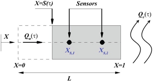
The one-dimensional ablating material heated from one end surface while the other surface is exposed to a convective heat flux. The initial thickness of the slab is assumed to be $L_0$ at initial temperature distribution $T_0\left(x\right)$.

The heating process is subdivided into a sequence of three time steps: (i) the pre-ablation period ${\tau }_0<\tau <{\tau }_{\mathrm{ab},\mathrm{s}}$, (ii) the ablation period ${\tau }_{\mathrm{ab},\mathrm{s}}<\tau <{\tau }_{\mathrm{ab},\mathrm{f}}$ and (iii) the post-ablation period ${\tau }_{\mathrm{ab},\mathrm{f}}<\tau <{\tau }_{\mathrm{f}}$. Within the no-ablation periods, the moving boundary reaches a stationary state and the direct problem reduces to pure heat conduction problem. During the ablation period, the surface of ablating material is at the ablation temperature and the applied heat flux at $X=0$ serves to remove material from the heated surface which creates a moving boundary. The following formulas introduced in [27] are employed to nondimensionalize the governing equations as $\begin{array}{}X=\frac{x}{L},\tau =\frac{\alpha t}{L^2},\theta (X,\tau )=\frac{T(x,t)-T_0\left(x\right)}{T_{\mathrm{ab}}-T_0\left(x\right)}\end{array}$ $\begin{array}{}Q\left(\tau \right)=\frac{Lq\left(t\right)}{k\left[T_{\mathrm{ab}}-T_0\left(x\right)\right]},\lambda =\frac{H}{c_p\left[T_{\mathrm{ab}}-T_0\left(x\right)\right]},Bi=\frac{h_{\mathrm{\infty }}L}{k}\end{array}$ where $c_p$, $k$, $\alpha$ and $H$ are the specific heat, thermal conductivity, thermal diffusivity and ablation heat of ablating material, respectively. The mathematical formulations of ablation problem in dimensionless form are given by

No-ablation periods: (15a) $\frac{\mathrm{\partial }\theta }{\mathrm{\partial }\tau }=\frac{{\mathrm{\partial }}^2\theta }{\mathrm{\partial }{X}^2},\text{in}\begin{array}{c}\\ \end{array}0<X<1$(15a) (15b) $-\frac{\mathrm{\partial }\theta }{\mathrm{\partial }X}=Q_{\mathrm{a}}\left(\tau \right),\text{at}\begin{array}{c}\\ \end{array}X=\left\{\begin{array}{c}S\left({\tau }_0\right)\\ S\left({\tau }_{\mathrm{ab},\mathrm{f}}\right)\end{array}\begin{array}{c}\text{ for the pre-ablation period}\\ \text{ for the post-ablation period}\end{array}\right.$(15b) (15c) $-\frac{\mathrm{\partial }\theta }{\mathrm{\partial }X}=Q_{\mathrm{c}}(\tau \text{),}\text{at }X=1$(15c) (15d) $\theta ={\theta }_i(X,\tau ),\text{in}0<X<1.$(15d)

Ablation periods: (16a) $\frac{\mathrm{\partial }\theta }{\mathrm{\partial }\tau }=\frac{{\mathrm{\partial }}^2\theta }{\mathrm{\partial }{X}^2},\text{in}0<X<1$(16a) (16b) $\theta =1,\text{at}X=S\left(\tau \right)$(16b) (16c) $-\frac{\mathrm{\partial }\theta }{\mathrm{\partial }X}=Q_c(\tau \text{),}\text{at }X=1$(16c) (16d) $\theta ={\theta }_i(X,{\tau }_{\mathrm{ab}}),\text{in}0<X<1,$(16d) where $\theta (X,\tau )$ refers to the dimensionless temperature. The front surface position is determined from the energy balance equation at the ablating surface as (16e) $\begin{array}{c}\nu \frac{\text{d}S}{\text{d}\tau }=Q\left(\tau \right)+\frac{\mathrm{\partial }\theta \left(S\right(\tau ),\tau )}{\mathrm{\partial }X},\text{at}X=0.\\ \end{array}$(16e)

The ablation problem is solved by an implicit scheme using Landau transformation [25,31] to convert the moving boundary to the fixed boundary. The nonlinear character of the problem is handled by an iterative procedure at each time step.

6. Results and discussion

The efficiency and accuracy of the developed method in the improvement of the standard CGM are examined by a moving boundary ablation problem as benchmark. Teflon is considered as the ablating material with the constant thermal properties. The thermophysical properties of ablating material are presented in Table 1 [27].

Table 1. Thermophysical properties of ablating material.

Parameter	Typical value	Unit
k	0.22	W  m^−1 K^−1
α	9.11 × 10^−8	m^2 s^−1
H	44.7 × 10^8	J m^−3
Tab	833	K
T0	298	K

The simulation time is assumed to be 100 s. The initial and boundary conditions are summarized in Table 2.

Table 2. The initial and boundary conditions.

	Boundary conditions			Initial conditions
Parameter	qa,max	qc,max	T∞	T0	L0
Quantity	10^5W m^−^2	−2 × 10^4W m^−2	273 K	298 K	0.02 m

The spatial domain and the time duration are divided into 51 and 121 equally spaced intervals, respectively. Two test cases with different heat flux profiles are used: triangular profile and sinusoidal profile. Simulated measured temperatures are used to deal with the inverse problem. All numerical simulations are done in the presence of noise to investigate the stability of the proposed scheme; hereupon the standard deviation is taken as $\sigma =0.05$ (5% of the maximum measured temperature). The measurement containing random errors is as follows: (17) $Y_i\left(t\right)=Y_{\mathrm{exact},i}\left(t\right)+\omega \sigma ,\left(17\right)$(17) where subscript $\text{exact}$ shows the noiseless measurements, while subscript i is the number of sensor. The $\omega$ and $\sigma$ are random variable and standard deviation of the measurement errors, respectively.

To measure the temperature, two sensors are located inside the ablating material. The sensor position, $X_{S,1}$, depends on the front surface of ablating material. The front surface changes according to the applied heat flux profile at $X=0$. The positions of ablating material in the two test cases are presented in Table 3.

Table 3. Front surface of ablating materials.

Case number	Heat flux profile at X = 0	Heat flux profile at X = 1	Front position	Ablated thickness (mm)
Case 1	Triangular	Sinus	Xfp = 0.0103	Δx = 206
Case 2	Sinus	Triangular	Xfp = 0.0120	Δx = 0.240

Stand on the front location, the sensors are located inside the slab as X_S,1 = 0.02, X_S,2 = 0.95.

In the presented MCGM, the initial guess is taken as ${\mathbf{P}}^0=\left[\begin{array}{c}{Q}_{\mathrm{a}}\\ Q_{\mathrm{c}}\end{array}\right]$ at each time step. To improve the speed of the inverse technique, for $k=0$ the value of ${\mathbf{P}}^0$ is considered to be the predicted heat fluxes in the previous time step. The modified unknown vectors are built as ${\overline{\mathit{P}}}_1^k=\left[\begin{array}{c}{Q}_{\mathrm{a}}+i\mathrm{\Delta }{Q}_{\mathrm{a}}\\ Q_{\mathrm{c}}\end{array}\right]$ and ${\overline{\mathit{P}}}_2^k=\left[\begin{array}{c}{Q}_{\mathrm{a}}\\ Q_{\mathrm{c}}+i\mathrm{\Delta }{Q}_{\mathrm{c}}\end{array}\right]$. 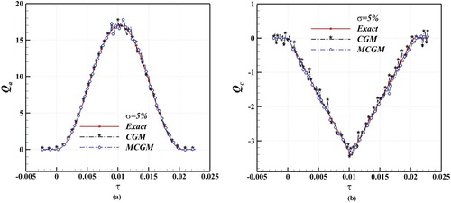The solution of direct problem for each of created vectors gives simultaneously the temperature field and the sensitivity with respect to that unknown. Figures 2(a,b) and 3(a,b) show the inverse solution of ablation problem by the implementation of the conventional and modified CGM. As depicted, the quality of the solution in comparison with the standard CGM is maintained as the MCGM is utilized. Considering noisy temperature results in oscillations in the inverse solution and it creates instabilities as shown in Figures 2(a,b) and 3(a,b). The perturbations are more pronounced during the ablation period.

Figure 2. Solution of inverse problem with noisy measurements for the first case under the study: (a) triangular profile for applied heat flux Q_a and (b) sinusoidal profile for convective heat flux Q_c.

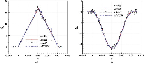
Figure 3. Solution of inverse problem with noisy measurements for the second case under the study: (a) sinusoidal profile for applied heat flux Q_a and (b) triangular profile for convective heat flux Q_c.

Figures 4(a,b) and 5(a,b) demonstrate the convergence rate of the inverse solution process at two different time steps. The progress in convergence speed of computational simulation is obviously depicted.

Figure 4. The variation of convergence rate versus the required iteration number at two different time steps: (a) 70th time step and (b) 90th time step for the first case under the study.

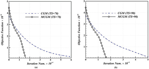
Figure 5. The variation of convergence rate versus the required iteration number at two different time steps: (a) 70th time step and (b) 90th time step for the second case under the study.

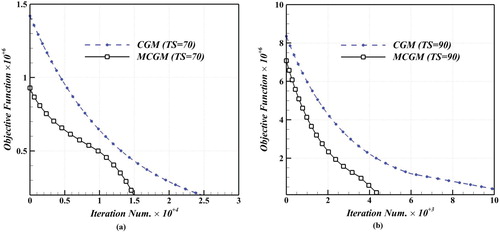
The simultaneous solution of direct and sensitivity problems in conjunction with the circumvention of the computation of sensitivity coefficients by using the CVDM affect the standard CGM solution procedure remarkably.

Table 4 shows the CPU run time for the test cases under the study. The required number of iterations and the computational expenses increased for the cases with more excursions and fluctuations.

Table 4. CPU run time for different test cases.

	σ = 0.05
	Case 1	Case 2
CGM	4169.54 s	3411.34 s
MCGM	1727.02 s	1562.30 s

For the sake of quantitative comparison, the accuracy and effectiveness of the developed scheme are investigated by the root mean square deviation (RMSD). The RMSD is defined as follows: (18) $E_{\mathrm{RMS}}=\sqrt{\frac{1}{P}\sum _{p=1}^P{\left(Q_{\mathrm{com},p}-Q_{\mathrm{exa},p}\right)}^2}.\left(18\right)$(18)

As shown in Table 5, the computed RMSDs are still in an acceptable range even though the noisy measurements are utilized.

Table 5. RMSD of estimated heat flux values.

	σ = 0.05
	Case 1		Case 2
	Qa	Qc	Qa	Qc
CGM	0.4363	0.1001	0.2712	0.1015
MCGM	0.3386	0.0492	0.2887	0.0682

7. Conclusion

Besides the robustness of the conventional CGM and its vast applications in dealing with the variety of inverse analyses, a weak point of the standard CGM is the huge number of required iterations in a solution of nonlinear problems. In general, the coupled governing equations in nonlinear problems increase the complexity of this class of inverse problems and enhance the computational expenses remarkably. To treat this problem and improve the efficiency of the standard CGM, several schemes such as exact calculation of sensitivity coefficients and utilizing the relaxation factor were proposed. This study represents a novel scheme to speed up the conventional CGM by merging the different steps in the computational algorithm to reduce the required mathematical manipulations. To meet this goal, the direct and sensitivity problems are solved simultaneously by using the CVDM. Furthermore, obtaining and solving the sensitivity problem is circumvented by this approach. The accuracy of the developed technique is examined by moving boundary ablation problem. The calculated results illustrate the efficiency and accuracy of the presented method.

Disclosure statement

No potential conflict of interest was reported by the authors.

References

- Lemos LD, Brittes R, França FH. Application of inverse analysis to determine the geometric configuration of filament heaters for uniform heating. Int J Therm Sci. 2016;105:1–12. doi: 10.1016/j.ijthermalsci.2016.02.015
- Najafi H, Woodbury KA, Beck JV. Real time solution for inverse heat conduction problems in a two-dimensional plate with multiple heat fluxes at the surface. Int J Heat Mass Transf. 2015;91:1148–1156. doi: 10.1016/j.ijheatmasstransfer.2015.08.020
- Molavi H, Hakkaki-Fard A, Molavi M, et al. Estimation of boundary conditions in the presence of unknown moving boundary caused by ablation. Int J Heat Mass Transf. 2011;54(5):1030–1038. doi: 10.1016/j.ijheatmasstransfer.2010.11.035
- Payan S, Sarvari SMH, Behzadmehr A. Inverse boundary design Radiation problem within combustion enclosures with absorbing-emitting non-gray media. Num Heat Transfer Part A: Appl. 2014;65:1114–1137. doi: 10.1080/10407782.2013.851572
- Farzan H, Sarvari SH, Mansouri S. Inverse boundary design of a radiative smelting furnace with ablative phase change phenomena. Appl Therm Eng. 2016;98:1140–1149. doi: 10.1016/j.applthermaleng.2016.01.029
- Najafi H, Woodbury KA, Beck JV. A filter based solution for inverse heat conduction problems in multi-layer mediums. Int J Heat Mass Transf. 2015;83:710–720. doi: 10.1016/j.ijheatmasstransfer.2014.12.055
- Ozisik MN. Inverse heat transfer: fundamentals and applications. New York: CRC Press; 2000.
- Beck JV, Blackwell B, Clair Jr CRS. Inverse heat conduction: ill-posed problems. New York: James Beck; 1985.
- Cui M, Zhu Q, Gao X. A modified conjugate gradient method for transient nonlinear inverse heat conduction problems: a case study for identifying temperature-dependent thermal conductivities. J Heat Transfer. 2014;136(9):091301–091307. doi: 10.1115/1.4027771
- Cui M, Duan W-w, Gao X-w. A new inverse analysis method based on a relaxation factor optimization technique for solving transient nonlinear inverse heat conduction problems. Int J Heat Mass Transf. 2015;90:491–498. doi: 10.1016/j.ijheatmasstransfer.2015.07.009
- Beck JV, Woodbury KA. Inverse heat conduction problem: sensitivity coefficient insights, filter coefficients, and intrinsic verification. Int J Heat Mass Transf. 2016;97:578–588. doi: 10.1016/j.ijheatmasstransfer.2016.02.034
- Woodbury KA, Najafi H, Beck JV. Exact analytical solution for 2-D transient heat conduction in a rectangle with partial heating on one edge. Int J Therm Sci. 2017;112:252–262. doi: 10.1016/j.ijthermalsci.2016.10.014
- Sarvari SMH, Mansouri SH, Howell JR. Inverse design of three-dimensional enclosures with transparent and absorbing-emitting media using an optimization technique. Int Commun Heat Mass Transfer. 2003;30(3):149–162. doi: 10.1016/S0735-1933(03)00026-5
- Sarvari SMH, Howell JR. A general method for estimation of boundary conditions over the surface of shields surrounding by radiating enclosures numerical heat transfer. Num Heat Transfer Part B Fundamentals. 2003;44:25–43. doi: 10.1080/713836332
- Hu J, Gao X. Development of complex-variable differentiation method and its application in isogeometric analysis. Aust J Mech Eng. 2013;11(1):37–43. doi: 10.7158/M12-052.2013.11.1
- Yu X, Bai Y, Cui M, et al. Inverse analysis of thermal conductivities in transient non-homogeneous and non-linear heat conductions using BEM based on complex variable differentiation method. Sci China Phys. Mech Astron. 2013;56(5):966–973. doi: 10.1007/s11433-013-5064-y
- Cui M, Gao X, Chen H. A new inverse approach for the equivalent gray radiative property of a non-gray medium using a modified zonal method and the complex-variable-differentiation method. J Quant Spectrosc Radiat Transfer. 2011;112(8):1336–1342. doi: 10.1016/j.jqsrt.2011.01.029
- Cui M, Gao X, Zhang J. A new approach for the estimation of temperature-dependent thermal properties by solving transient inverse heat conduction problems. Int J Therm Sci. 2012;58:113–119. doi: 10.1016/j.ijthermalsci.2012.02.024
- Cui M, Yang K, Xu X-l, et al. A modified Levenberg–Marquardt algorithm for simultaneous estimation of multi-parameters of boundary heat flux by solving transient nonlinear inverse heat conduction problems. Int J Heat Mass Transfer. 2016;97:908–916. doi: 10.1016/j.ijheatmasstransfer.2016.02.085
- Cui M, Zhao Y, Xu B, et al. A new approach for determining damping factors in Levenberg–Marquardt algorithm for solving an inverse heat conduction problem. Int J Heat Mass Transfer. 2017;107:747–754. doi: 10.1016/j.ijheatmasstransfer.2016.11.101
- Lai K-L, Crassidis JL, editors. Generalizations of the complex-step derivative approximation. In AIAA Guidance, Navigation, and Control Conference, Keystone, CO; 2006.
- Martins JR, Sturdza P, Alonso JJ. The complex-step derivative approximation. ACM Trans Math Softw TOMS. 2003;29(3):245–262. doi: 10.1145/838250.838251
- Lyness JN, Moler CB. Numerical differentiation of analytic functions. SIAM J Numer Anal. 1967;4(2):202–210. doi: 10.1137/0704019
- Cui M, Li N, Liu Y, et al. Robust inverse approach for two-dimensional transient nonlinear heat conduction problems. J Thermophys Heat Transfer. 2015;29(2):253–262. doi: 10.2514/1.T4323
- Mitchell SL, Myers TG. Heat balance integral method for one-dimensional finite ablation. J Thermophys Heat Transfer. 2008;22(3):508–514. doi: 10.2514/1.31755
- Ozisik MN. Heat conduction. New York: John Wiley & Sons; 1993.
- Farzan H, Loulou T, Sarvari SH. Estimation of applied heat flux at the surface of ablating materials by using sequential function specification method. J Mech Sci Technol. 2017;31(8):3969–3979. doi: 10.1007/s12206-017-0744-6
- Hoffmann KA. Computational fluid dynamics for engineers. Austin (TX): Engineering Education System; 1989.
- Anderson DA, Tannehill JC, Pletcher RH. Computational fluid mechanics and heat transfer; 1984.
- Versteeg HK, Malalasekera W. An introduction to computational fluid dynamics: the finite volume method. New York: Pearson Education; 2007.
- Blackwell B, Hogan R. One-dimensional ablation using Landau transformation and finite control volume procedure. J Thermophys Heat Transfer. 1994;8(2):282–287. doi: 10.2514/3.535