The uncertainty analysis in linear and nonlinear regression revisited: application to concrete strength estimation

ABSTRACT

Regression is a common technique in engineering when physical laws are unknown. Practitioners usually look for a unique set of true parameters that optimally explain the observed data. This is, for instance, the case in concrete strength estimation where engineers have been looking for an universal law to estimate this magnitude. We show that this approach is incorrect if the uncertainty of the regression problem is not properly taken into account. The uncertainty analysis of linear regression problems is revisited providing an analytical expression for the direction of maximum uncertainty where most of the models are sampled when partial information is used. We also analyse the case of 1D nonlinear regression models (exponential and potential models) and the multivariate case. We show a simple way of sampling the posterior distribution of the model parameters by performing least-squares of different data bags (bootstrap), introducing the percentile curves for the concrete strength estimation, comparing the results obtained from the linearized and nonlinear bootstrap procedures in the case of the nonlinear regression models. The methodology introduced in this paper constitutes a robust and simple way of assessing the intrincic uncertainty of these well-known parameter identification problems and adopting more robust decisions.

KEYWORDS:

• Experimental models
• linear regression
• uncertainty analysis
• concrete strength estimation

SUBJECT CLASSIFICATION CODES:

• 65.3X 40-58
• 65 59
• 68.0X 40-58
• 68 73
• 62 59

1. Introduction

Inverse problems is a discipline of applied mathematics that has many applications in science and engineering. Most of the inverse problems in geosciences can be written in discrete form $\mathbf{\text{F}}\left(\mathbf{\text{m}}\right)=\mathbf{\text{d}}.$ In this relationship $\mathbf{\text{m}}=\left(m_1,m_2,\dots ,m_n\right)\in M\subset {\mathbb{R}}^{\mathrm{n}}$ is the estimated model (or model parameters) that belongs to a set of admissible models $M$ defined in terms of some prior knowledge, $\mathbf{\text{d}}\in {\mathbb{R}}^{\mathrm{s}}$ are the observed data, and $\mathbf{\text{F}}\left(\mathbf{\text{m}}\right)=\left(f_1\left(\mathbf{\text{m}}\right),f_2\left(\mathbf{\text{m}}\right),\dots f_s\left(\mathbf{\text{m}}\right)\right)$ is the vector field representing the forward model, being $f_j\left(\mathbf{\text{m}}\right)$ the j-scalar field component function of $\mathbf{\text{F}}$, accounting for the j-th data.

The inverse problem consists in finding the models $\mathbf{\text{m}}$ whose predictions $\mathbf{\text{F}}\left(\mathbf{\text{m}}\right)$ accurately match the observed data $\mathbf{\text{d}}$, and are ill-posed, that is, either the inverse problem does not admit solution, either the solution is not unique, or it is unstable, that is, the solution does not depend continuously on the observed data (ill-conditioned problem). Uncertainty analysis consists in sampling the family of models $\mathbf{\text{m}}\in {\mathbb{R}}^{\mathrm{s}}$ that fit the observed data $\mathbf{\text{d}}\in {\mathbb{R}}^{\mathrm{s}}$ within the same error bounds $||\mathbf{\text{F}}\left(\mathbf{\text{m}}\right)-\mathbf{\text{d}}|{|}_2^{}<tol,$ and are compatible with the prior information at disposal, if any. These models are called equivalent.

It has been shown that the topography of the data error cost function corresponds to a straight flat elongated valley if the inverse problem is linear, whereas in the nonlinear case, the cost function topography consists of one or more curvilinear valleys (or basins) of low misfits, eventually connected by saddle points [1,2]. Besides, in the linear case, the equivalent models belong to the linear hyper quadric whose axes and orientations are related to the ill-conditioning of the system matrix. This theoretical development complements the stochastic approach of inverse problems originally proposed by Tarantola and Valette [3,4], showing that the uncertainty region of linear and nonlinear inverse problems has a mathematical structure that is embedded in the forward physics $\mathbf{\text{F}}$ and also in the observed data. In addition, the noise in the data perturbs the least-squares solution and the size of the linear and nonlinear uncertainty regions for the same value of the data misfit (see Fernández Martínez et al. [21,22] for more details). Therefore, uncertainty analysis and model appraisal is always a necessary step in inversion and parameter identification problems (see for instance [5,6]). Despite its importance, these results are barely known in the engineering community.

2. Problem statement in the application domain on non-destructive concrete strength estimation

The research presented in this paper has been practically inspired by the need of concrete specialists to have a reliable methodology for assessing concrete strength from non-destructive measurements. Assessing the concrete strength of existing buildings is a common engineering activity which is driven, among other reasons, by the need of structural seismic retrofitting where the load capacity must be checked or improved [7].

Non-destructive measurements based strength evaluation is justified by the fact that: (a) taking cores for assessing directly strength from theses samples is expensive and time-consuming, (b) it can induce some damage in the structures and sometimes even put it at risk, (c) non-destructive test results are supposed to be correlated with concrete strength. This correlation has been justified by physical reasons for several non-destructive techniques among which velocity of ultrasonic waves, which is directly correlated with the elastic rigidity of the material, and rebound number, measured after the impact of a steel ball on the concrete surface, which is correlated with the material hardness [8]. However, this correlation is not perfect since many other parameters can influence the relation between the non-destructive test result and the strength (humidity, type of aggregates, carbonation …).

Therefore it is required to identify an empirical ‘conversion’ (or regression) models, which makes possible to derive strength estimates from the non-destructive test results, for instance, rebound measurements [9] or ultrasonic pulse velocity measurements [10]. The researchers in this engineering field as in other similar fields (forestry, petroleum exploration, mining, etc.) are usually looking for empirical laws that relate these parameters. The same methodology also applies to other construction materials, such as masonry [11]. The common idea is that, once a conversion model $\text{y }=M\left(x\right)$ has been identified between a measured property $x$ (typically the result of non-destructive technique) and a required target $y$ (typically the material strength), this mathematical model can be used to estimate $y$ for new values of $x$ where the value of $y$ has not been measured.

The different steps of the conversion model identification have been recently described into details in Breysse et al. [12]. Linear empirical relationships are commonly established and the researchers in this field are often looking for a hypothetical universal relationship [8]. The accuracy of the assessed strength highly depends on the accuracy and relevancy of the prediction model. Relevancy means that the model must be used in a context corresponding to that on which it has been validated. The accuracy of the model can be quantified through the goodness of fit between the predicted strengths and true strength values, for instance by quantifying the root mean squared error (RMS error). Thus, a key issue is the identification of adequate model parameters. The number of model parameters depends on the mathematical expression of the model, which is often two, for monovariate models, or three for bivariate models. If one takes, for instance, the example of prediction of concrete strength $r$ from rebound hammer measurements $R$, a literature review has shown that a variety of mathematical expressions can be used by researchers [8]. The most common ones being linear models ($r\ast \left(R\right)=a_0+a_{1}R$ [13]), power models ($r\ast \left(R\right)=a_0{R}^{a_1}$ [14]) and exponential models ($r\ast \left(R\right)=a_0{e}^{a_{1}R}$ [9]). A similar statement can be done for prediction models based on other non-destructive techniques, like ultrasonic pulse velocity $V$, replacing the rebound hammer, $R$, in the above expressions [15]. Whatever the case, the identification problem comes to find the best estimates $a_0^{est}$ and $a_1^{est}$ for the two model parameters. Bilinear estimators of the kind $r\ast \left(R,V\right)=a_0+a_{1}R+a_{2}V,$ are also used in common practice [16] in order to try to reduce uncertainty in the estimation of the concrete strength by introducing different correlated variables to the output variable, $r\ast$. For any given dataset made of $N$ pairs $\left(r_i,V_i\text{, }{\text{R}}_i\right),i=1,\dots ,N$, these estimates will correspond to the minimization of the RMS error referred above.

Despite the huge number of research works in the domain on non-destructive testing applied to concrete, some important issues justify the original developments proposed in this paper. There is no consensus between experts about how a conversion model must be chosen and or calibrated and various options can be considered [17], while their advantages and drawbacks have been analysed only very recently [18].

The common engineering practice is unfortunately limited to the model calibration stage, i.e. to the identification of the estimates of model parameters, without considering the effective ability of the model to estimate strength at locations which have not been used during the parameter identification stage. In other words, only the fitting error is quantified, and the effective prediction uncertainty remains unknown. An extensive literature review has shown that: (a) such universal relationship does not exist; (b) when analysing existing relations, a trade-off between the model parameters is revealed as a consistent pattern [19]. This trade-off has been explained by the fact that the model estimates can be viewed as the solution of an inverse problem with a given uncertainty space that causes each single identification problem to drive to new estimates. Besides, while looking at how this problem is commonly treated, several factors exist which have a significant influence on the quality of the regression model, and therefore on the magnitude of the prediction error on strength. These factors have been recently listed in M. Alwash et al. [20], and include the dataset size, the magnitude of the data uncertainty, and the range of variation of the parameter to be identified. The objective of this paper is to further analyse the identification stage in order to understand how these factors influence the uncertainty on strength estimates. On this basis, concrete experts will be able to justify a more robust methodology for on-site concrete strength estimates with NDT measurements, and to consider properly the uncertainty attached to this estimate.

In this paper, we revised the uncertainty in linear regression using linear algebra, providing an analytical expression for the direction of maximum uncertainty where most of the models of the linear regression problem are sampled when partial information is used to achieve the regression. In the linear case, this direction implies a trade-off between the slope and the y-intercept of the least-squares regression line. We show that taking this trade-off into account it is possible to solve a one-parameter regression problem where the slope is the unique parameter to be identified, and its solution coincides with the regression line that is found via least-squares if first order approximations are considered. This analysis is also performed for two different 1D nonlinear regression models (exponential and potential models) and for the multivariate case (bilinear). We illustrate this analysis with a practical example consisting of the concrete strength assessment by means of non-destructive measurements, showing the existing trade-off among the parameters of these empirical relationships between Non-Destructive Technique (NDT) measurement and the concrete strength. We show that the use of partial data information (sampling of the data space) greatly influences the model parameters that are inverted along the direction of maximum anisotropy. Therefore, no universal relationship can be found for the linear regression. In conclusion the problem does not reside in finding the least-squares solution that coincides with the maximum likelihood solution in Bayesian approaches, but to appraise this solution in order to quantify uncertainty introduced by partial data knowledge, noise in data gathering and/or also wrong modelling assumptions, since the correct regression model is a priori unknown, and in any case it is a simplification of the reality.

3. The algebraic interpretation of a simple linear regression problem

In this section, we present the analytic formulas for the uncertainty region of a simple linear regression problem of the kind $y^{\ast }\left(x\right)=a_0+a_{1}x$ to the experimental data table given by: $\left\{\left(x_1,y_1\right),\left(x_2,y_2\right),\dots ,\left(x_m,y_m\right)\right\}.$

As it is very well-known, the problem consists of finding the parameters ${\mathbf{\text{m}}}^{\mathrm{T}}=\left(a_0,a_1\right)$ so that the distance between the observed data $\mathbf{\text{y}}=\left(\begin{array}{c}{y}_1\\ y_2\\ ⋮\\ y_m\end{array}\right)$ and the corresponding predictions ${\mathbf{\text{y}}}^{pre}=\left(\begin{array}{c}{y}_1^{\ast }\\ y_2^{\ast }\\ ⋮\\ y_m^{\ast }\end{array}\right)$ is minimum according to the Euclidean distance in the data space ${\mathbb{R}}^m$.

The vector of predictions can be written ${\mathbf{\text{y}}}^{pre}=a_0{\mathbf{\text{1}}}_{{\mathbb{R}}^m}+a_1\mathbf{\text{x}}$ and belongs therefore to the subspace of predictions $Col\left(\mathbf{\text{F}}\right)=⟨{\mathbf{\text{1}}}_{{\mathbb{R}}^m},\mathbf{\text{x}}⟩$ which is the column space of the forward operator $\mathbf{\text{F}}=\left[{\mathbf{\text{1}}}_{{\mathbb{R}}^m}\mathbf{\text{x}}\right].$ The fact that the observed data does not belong to subspace $Col\left(\mathbf{\text{F}}\right)$, makes the linear system $\mathbf{\text{F}}\mathbf{\text{m}}=\mathbf{\text{y}}$ have no solution. Hence, the problem is solved in the least-squares sense, that is, finding ${\mathbf{\text{m}}}_{LS}$ so that the prediction error $||\mathbf{\text{F}}{\mathbf{\text{m}}}_{LS}-\mathbf{\text{y}}|{|}_2$ is the minimum. For this purpose, $\mathbf{\text{F}}{\mathbf{\text{m}}}_{LS}$ is needed to coincide with the orthogonal projection of $\mathbf{\text{y}}$ onto $Col\left(\mathbf{\text{F}}\right)$: (1) $\mathbf{\text{F}}{\mathbf{\text{m}}}_{LS}={\text{Proj}}_{Col\left(\mathbf{\text{F}}\right)}^{\mathrm{\perp }}\left(\mathbf{\text{y}}\right).$(1) Consequently, the prediction error $\mathbf{\text{E}}=\mathbf{\text{F}}{\mathbf{\text{m}}}_{LS}-\mathbf{\text{y}}$ belongs to the null space of the adjoint operator ${\mathbf{\text{F}}}^{\mathrm{T}}$, $\ker \left({\mathbf{\text{F}}}^{\mathrm{T}}\right)$, providing the normal equations: (2) ${\mathbf{\text{F}}}^{\mathrm{T}}\left(\mathbf{\text{F}}{\mathbf{\text{m}}}_{LS}-\mathbf{\text{y}}\right)={\mathbf{\text{0}}}_{{\mathbb{R}}^m}\iff {\mathbf{\text{F}}}^{\mathrm{T}}\mathbf{\text{F}}{\mathbf{\text{m}}}_{LS}={\mathbf{\text{F}}}^{\mathrm{T}}\mathbf{\text{y}}$(2)

The matrix ${\mathbf{\text{F}}}^{\mathrm{T}}\mathbf{\text{F}}$ is square of size 2, symmetric, and has the same rank as $\mathbf{\text{F}}$. As a consequence, this linear system has a unique solution in the case of purely overdetermined linear systems, that is, if the number of data m is greater than 2 and the rank of $\mathbf{\text{F}}$ is 2. The least-squares solution writes: (3) ${\mathbf{\text{m}}}_{LS}=\left(\begin{array}{c}{a}_0^{LS}\\ a_1^{LS}\end{array}\right)=({\mathbf{\text{F}}}^{\mathrm{T}}\mathbf{\text{F}}{)}^{-1}{\mathbf{\text{F}}}^{\mathrm{T}}\mathbf{\text{y}}.$(3) being the system matrix of (2) in this case: (4) ${\mathbf{\text{F}}}^{\mathrm{T}}\mathbf{\text{F}}=\left(\begin{array}{cc}m& \sum _{k=1}^m{x}_k\\ \sum _{k=1}^m{x}_k& \sum _{k=1}^m{x}_k^2\end{array}\right).$(4)

The least-squares solution can be analytically written as follows: (5) $\begin{array}{rl}{a}_0^{LS}& ={\mu }_y-{\mu }_x{a}_1^{LS},\\ a_1^{LS}& =\frac{\mathrm{cov}\left(\mathbf{\text{y}},\mathbf{\text{x}}\right)}{\mathrm{var}\left(\mathbf{\text{x}}\right)},\end{array}$(5) where ${\mu }_y$ represents the arithmetic mean of the components of the observed data $\mathbf{\text{y}}$, ${\mu }_x$ the arithmetic mean of $\mathbf{\text{x}}$, $\mathrm{var}\left(\mathbf{\text{x}}\right)$ is the variance of the random variable $\mathbf{\text{x}}$, and $\mathrm{cov}\left(\mathbf{\text{y}},\mathbf{\text{x}}\right)$ the covariance between the random variable $\mathbf{\text{x}}$ and the observed data $\mathbf{\text{y}}$. Taking formula (5) into account, the regression straight line writes: (6) $y-{\mu }_y=\frac{\mathrm{cov}\left(\mathbf{\text{y}},\mathbf{\text{x}}\right)}{\mathrm{var}\left(\mathbf{\text{x}}\right)}\left(x-{\mu }_x\right).$(6)

Matrix ${\mathbf{\text{F}}}^{\mathrm{T}}\mathbf{\text{F}}$ admits orthogonal diagonalization, as follows: (7) ${\mathbf{\text{F}}}^{\mathrm{T}}\mathbf{\text{F}}=\mathbf{\text{V}}\mathbf{\text{D}}{\mathbf{\text{V}}}^{\mathrm{T}}=\left[{\mathbf{\text{v}}}_1{\mathbf{\text{v}}}_2\right]\left[\begin{array}{cc}{\lambda }_1& 0\\ 0& {\lambda }_2\end{array}\right]\left[\begin{array}{c}{\mathbf{\text{v}}}_1^{\mathrm{T}}\\ {\mathbf{\text{v}}}_2^{\mathrm{T}}\end{array}\right],{\lambda }_1,{\lambda }_2\in \mathbb{R},{\lambda }_1>{\lambda }_2>0.$(7) Besides, using the singular value decomposition, $\mathbf{\text{F}}=\mathbf{\text{U}}\mathbf{\Sigma }{\mathbf{\text{V}}}^{\mathrm{T}}$, the least-squares solution in expression (3), can be written as follows: (8) ${\mathbf{\text{m}}}_{LS}=\mathbf{\text{V}}{\mathbf{\text{D}}}^{-1}{\mathbf{\Sigma }}^{\mathrm{T}}{\mathbf{\text{U}}}^{\mathrm{T}}\mathbf{\text{y}}=\frac{y_{u1}}{\sqrt{{\lambda }_1}}{\mathbf{\text{v}}}_1+\frac{y_{u2}}{\sqrt{{\lambda }_2}}{\mathbf{\text{v}}}_2,$(8) where $y_{u1},y_{u2}$ are the two first coordinates of vector $\mathbf{\text{y}}$ in the $\left\{{\mathbf{\text{v}}}_1,{\mathbf{\text{v}}}_2\right\}$ basis. Expression (8) serves to explain that the least-squares solution can be expanded as a linear combination of the eigenvectors of the column correlation matrix of $\mathbf{\text{F}},{\mathbf{\text{F}}}^{\mathrm{T}}\mathbf{\text{F}}.$ Therefore the least square solution will change when a partial subset of the data (called a data bag) is considered. We will numerically show that this iterative bagging procedure serves to sample the uncertainty region of the linear regression problem, following the direction of maximum uncertainty, ${\mathbf{\text{v}}}_2$, associated to the smaller eigenvalue ${\lambda }_2$.

4. The uncertainty region in linear inverse problems

The uncertainty region of the linear regression problem is: (9) $M_{tol}=\left\{\mathbf{\text{m}}:{||\mathbf{\text{F}}\mathbf{\text{m}}-\mathbf{\text{y}}||}_2\le tol\right\},$(9) and coincides with the region of the model space inside the ellipse: (10) ${\mathbf{\text{m}}}^{\mathrm{T}}{\mathbf{\text{F}}}^{\mathrm{T}}\mathbf{\text{F}}\mathbf{\text{m}}-2{\mathbf{\text{m}}}^{\mathrm{T}}{\mathbf{\text{F}}}^{\mathrm{T}}\mathbf{\text{y}}+{\mathbf{\text{y}}}^{\mathrm{T}}\mathbf{\text{y}}=to{l}^2,$(10) that it is centred in the least-squares solution and oriented in the direction of the eigenvectors of ${\mathbf{\text{F}}}^{\mathrm{T}}\mathbf{\text{F}}$. Hence, referred to its principal axes (provided by the $\mathbf{\text{V}}$ basis) this ellipse is: (11) $\frac{{\left(a_{0V}-a_{0V}^{LS}\right)}^2}{{\left(\frac{tol}{\sqrt{{\lambda }_1}}\right)}^2}+\frac{{\left(a_{1V}-a_{1V}^{LS}\right)}^2}{{\left(\frac{tol}{\sqrt{{\lambda }_2}}\right)}^2}=1.$(11) A theoretical analysis of the uncertainty in linear and nonlinear inverse problems is shown in Fernández Martínez et al. [1,2]. Besides, the effect of noise and that of the regularization is provided in Fernández Martínez et al. [21,22], showing how the noise affects the size of uncertainty region in linear and nonlinear inverse problems, and the effect of the regularization in estabilizing the inversion through local optimization methods. Nevertheless, despite of the regularization, the equivalent models do not vanish. Therefore, the uncertainty analysis in linear and nonlinear inverse problems for model quality assessment is always needed.

The statistical approach of uncertainty in linear inverse problems can be consulted for instance in C. Aster et al. [23], and it is based on the fact that squared data prediction error $||\mathbf{\text{F}}\mathbf{\text{m}}-\mathbf{\text{y}}|{|}_2^2$ follows a ${\chi }^2$ distribution with $m-n$ degrees of freedom. That way a p-value test can be performed to analyse if the least-squares solution produces an acceptable data fit and if the statistical assumptions of data errors are consistent. Wrong models produce extraordinarily small p-values (e.g. 10⁻¹²). If the p-value is close to 1, the fit of the model predictions to the data is almost exact. This approach also allows us to find the confidence regions that are related to the region of uncertainty stated in Fernández Martínez et al. [1]. In addition to this, it is possible to show that ${\mathbf{\text{F}}}^{\mathrm{T}}\mathbf{\text{F}}$ is the inverse of the posterior covariance matrix between model parameters (see for instance [23]). An alternative approach consists in solving the orthogonal distance regression problem, as shown in J. Mandel [24], and E. Cruz and P. Fernandes [25].

Continuing with the linear algebra approach of the simple linear regression problem, let us call: (12) $S=\sum _{k=1}^m{x}_k=m{\mu }_x,S_c=\sum _{k=1}^m{x}_k^2=m{\mu }_{x^2},$(12) then, the matrix (13) ${\mathbf{\text{F}}}^{\mathrm{T}}\mathbf{\text{F}}=\left(\begin{array}{cc}m& S\\ S& S_c\end{array}\right),$(13) has the following eigenvalues: (14) $\begin{array}{rl}{\lambda }_1& =\frac{\left(S_c+m\right)+S_c\sqrt{{\left(1-\frac{m}{S_c}\right)}^2+4\frac{S^2}{S_c^2}}}{2}=m\frac{{\mu }_{x^2}+1+\sqrt{{\left({\mu }_{x^2}-1\right)}^2+4{\mu }_x^2}}{2},\\ {\lambda }_2& =\frac{\left(S_c+m\right)-S_c\sqrt{{\left(1-\frac{m}{S_c}\right)}^2+4\frac{S^2}{S_c^2}}}{2}=m\frac{{\mu }_{x^2}+1-\sqrt{{\left({\mu }_{x^2}-1\right)}^2+4{\mu }_x^2}}{2}.\end{array}$(14) The corresponding eigenvectors ${\mathbf{\text{v}}}_i\in \ker ({\mathbf{\text{F}}}^{\mathrm{T}}\mathbf{\text{F}}-{\lambda }_i{I}_2)=\left(S,{\lambda }_i-m\right)$ are orthogonal since they are associated with different eigenvalues of a symmetric matrix, and the following relationship holds: (15) $S^2+\left({\lambda }_i-m\right)\left(S_c-{\lambda }_i\right)=0.$(15)

The region of uncertainty for an absolute error value $tol$ is the ellipse with the minimum axis (and minimum uncertainty) in the direction of ${\mathbf{\text{v}}}_1=⟨\left(S,{\lambda }_1-m\right)⟩$ and length $tol/\phantom{tol\sqrt{{\lambda }_1}}\sqrt{{\lambda }_1}$, and maximum axis (and maximum uncertainty) in the direction of ${\mathbf{\text{v}}}_2=⟨\left(S,{\lambda }_2-m\right)⟩$ and length $tol/\phantom{tol\sqrt{{\lambda }_2}}\sqrt{{\lambda }_2}$.

Both eigenvalues can be approximated using Taylor’s first order approximation as follows: (16) ${\tilde{\lambda }}_1=\frac{\left(S_c+m\right)+S_c\left[1-{\displaystyle \frac{m}{S_c}}+{\displaystyle \frac{m^2}{2S_c^2}}+{\displaystyle \frac{2S^2}{S_c^2}}\right]}{2}=m\left({\mu }_{x^2}+\frac{{\mu }_x^2}{{\mu }_{x^2}}+\frac{1}{4{\mu }_{x^2}}\right),$(16) (17) ${\tilde{\lambda }}_2=\frac{\left(S_c+m\right)-S_c\left[1-{\displaystyle \frac{m}{S_c}}+{\displaystyle \frac{m^2}{2S_c^2}}+{\displaystyle \frac{2S^2}{S_c^2}}\right]}{2}=m\left(1-\frac{{\mu }_x^2}{{\mu }_{x^2}}-\frac{1}{4{\mu }_{x^2}}\right).$(17)

The condition number and its approximated value are: (18) $\begin{array}{rl}\kappa & =\sqrt{\frac{{\lambda }_1}{{\lambda }_2}}=\sqrt{\frac{S_c^2+m^2+2S^2+\left(S_c+m\right)S_c\sqrt{{\left(1-\frac{m}{S_c}\right)}^2+4{\displaystyle \frac{S^2}{S_c^2}}}}{2m{S}_c-2S^2}}\simeq \\ & \simeq \sqrt{{\mu }_{x^2}+{\mu }_x^2+\frac{{\mu }_x^2+{\mu }_x^4}{{\mu }_{x^2}-{\mu }_x^2}.}\end{array}$(18) Furthermore, the equations of the axis of the ellipse of uncertainty are:

1. Axis of minimum uncertainty (associated to the biggest eigenvalue): (19) $a_1-a_1^{LS}=p_1\left(a_0-a_0^{LS}\right).$(19)

2. Axis of maximum uncertainty (associated with the smallest eigenvalue): (20) $a_1-a_1^{LS}=p_2\left(a_0-a_0^{LS}\right).$(20)

The true and simplified slope values of the axes of uncertainty are: (21) $\begin{array}{rl}{p}_1& =\frac{{\lambda }_1-m}{S},{\tilde{p}}_1=\frac{S_c-m}{S}\simeq \frac{S_c}{S}=\frac{{\mu }_{x^2}}{{\mu }_x},\\ p_2& =\frac{{\lambda }_2-m}{S},{\tilde{p}}_2=-\frac{S}{S_c-m}-\frac{m}{S}\simeq -\frac{S}{S_c}=-\frac{{\mu }_x}{{\mu }_{x^2}}.\end{array}$(21) This simplification holds if $S_c>>S$ and $S>>m$.

This is an interesting result since the slope of the axis of the ellipse of uncertainty is mainly controlled by the ratio of two terms of the matrix ${\mathbf{\text{F}}}^{\mathrm{T}}\mathbf{\text{F}}$. The fact that ${\lambda }_2<<{\lambda }_1$ provokes the uncertainty region to be elongated in the direction of the eigenvector ${\mathbf{\text{v}}}_2$. Most of the equivalent models are sampled along this axis, and are therefore related as follows: (22) $a_1=a_1^{LS}+p_2\left(a_0-a_0^{LS}\right)=a_1^{LS}-p_2{a}_0^{LS}+p_2{a}_0.$(22) Taking into account relationships (5) and (22), we reach: (23) $\begin{array}{rl}{a}_1^{LS}-a_0^{LS}{p}_2& =a_1^{LS}\left(1+p_2{\mu }_x\right)-p_2{\mu }_y=\\ & \simeq \frac{\mathrm{cov}\left(\mathbf{\text{y}},\mathbf{\text{x}}\right)}{\mathrm{var}\left(\mathbf{\text{x}}\right)}\left(1-\left(\frac{S}{S_c}+\frac{m^2}{4S_{c}S}\right){\mu }_x\right)+\left(\frac{S}{S_c}+\frac{m^2}{4S_{c}S}\right){\mu }_y\simeq \\ & \simeq \frac{\mathrm{cov}\left(\mathbf{\text{y}},\mathbf{\text{x}}\right)}{\mathrm{var}\left(\mathbf{\text{x}}\right)}\left(1-\frac{S}{S_c}{\mu }_x\right)+\frac{S}{S_c}{\mu }_y,\end{array}$(23) and (24) $p_2{a}_0\simeq -\left(\frac{S}{S_c}+\frac{m^2}{4S_{c}S}\right)a_0\simeq -\frac{S}{S_c}{a}_0.$(24) In a first approximation the equation of the axis of maximum uncertainty is: (25) $a_1\simeq \frac{\mathrm{cov}\left(\mathbf{\text{y}},\mathbf{\text{x}}\right)}{\mathrm{var}\left(\mathbf{\text{x}}\right)}\left(1-\frac{S}{S_c}{\mu }_x\right)+\frac{S}{S_c}{\mu }_y-\frac{S}{S_c}{a}_0.$(25)

Therefore, taking into account the existing trade-off relationship between $a_0$ and $a_1$, the simplified model of the simple regression using just one-parameter ($a_1$) is: (26) $y-{\mu }_y-\frac{\mathrm{cov}\left(\mathbf{\text{y}},\mathbf{\text{x}}\right)}{{\mu }_x}=a_1\left(x-{\mu }_x-\frac{\mathrm{var}\left(\mathbf{\text{x}}\right)}{{\mu }_x}\right).$(26)

Moreover, the same regression line without any simplification writes as follows: (27) $y-{\mu }_y+a_1^{LS}\left({\mu }_x+\frac{1}{p_2}\right)=a_1\left(x+\frac{1}{p_2}\right),$(27) where $p_2$ is the slope of the axis of maximum uncertainty stated in (21).

The parameter $a_1$ can be found by least-squares using the following expression: (28) $a_1=\frac{\left(\mathbf{\text{y}}-\left({\mu }_y+\frac{\mathrm{cov}\left(\mathbf{\text{y}},\mathbf{\text{x}}\right)}{{\mu }_x}\right)\mathbf{\text{1}}\right)\cdot \left(\mathbf{\text{x}}-\left({\mu }_x+\frac{\mathrm{var}\left(\mathbf{\text{x}}\right)}{{\mu }_x}\right)\mathbf{\text{1}}\right)}{\left(\mathbf{\text{x}}-\left({\mu }_x+\frac{\mathrm{var}\left(\mathbf{\text{x}}\right)}{{\mu }_x}\right)\mathbf{\text{1}}\right)\cdot \left(\mathbf{\text{x}}-\left({\mu }_x+\frac{\mathrm{var}\left(\mathbf{\text{x}}\right)}{{\mu }_x}\right)\mathbf{\text{1}}\right)}.$(28) In most of the practical cases, the expression (25) can be simplified as follows: (29) $a_1=\frac{\mathrm{cov}(\mathbf{\text{y}},\mathbf{\text{x}})}{\mathrm{var}\left(\mathbf{\text{x}}\right)},$(29) and the final one-parameter regression model writes: (30) $y-{\mu }_y-\frac{\mathrm{cov}\left(\mathbf{\text{y}},\mathbf{\text{x}}\right)}{{\mu }_x}=\frac{\mathrm{cov}(\mathbf{\text{y}},\mathbf{\text{x}})}{\mathrm{var}\left(\mathbf{\text{x}}\right)}\left(x-{\mu }_x-\frac{\mathrm{var}\left(\mathbf{\text{x}}\right)}{{\mu }_x}\right),$(30) which coincides with the least-squares regression line (6). This property means that (in first approximation) the standard regression line has the additional property of optimally taking into account the trade-off between the slope and the y-intercept of the regression line.

5. Nonlinear regression: the exponential model

A common nonlinear regression model is the exponential regression that consists of fitting the model $y^{\ast }\left(x\right)=a_0{e}^{a_{1}x}$ to the observed data. This nonlinear regression problem can be linearized by the logarithm parameterization: $\ln y^{\ast }\left(x\right)=\ln a_0+a_{1}x,$ which implies a linear regression of the observed data $\ln \mathbf{\text{y}}=\left(\begin{array}{c}\ln y_1\\ \ln y_2\\ ⋮\\ \ln y_m\end{array}\right)$ in $⟨{\mathbf{\text{1}}}_{{\mathbb{R}}^m},{\mathbf{\text{x}}}_{{\mathbb{R}}^m}⟩$. The vector of predictions $\ln {\mathbf{\text{y}}}^{pre}=\left(\begin{array}{c}\ln y_1^{\ast }\\ \ln y_2^{\ast }\\ ⋮\\ \ln y_m^{\ast }\end{array}\right)$ can be written as $\ln {\mathbf{\text{y}}}^{pre}=\ln a_0{\mathbf{\text{1}}}_{{\mathbb{R}}^m}+a_1\mathbf{\text{x}}$ and belongs to the subspace of predictions $⟨{\mathbf{\text{1}}}_{{\mathbb{R}}^m},\mathbf{\text{x}}⟩$ which is the column space of the forward operator $\mathbf{\text{F}}=\left[{\mathbf{\text{1}}}_{{\mathbb{R}}^m}\mathbf{\text{x}}\right].$ The system matrix of this linear regression problem has been stated in (4) and the relation between the parameters $\ln a_0^{LS}$ and $a_1^{LS}$ is: (31) $\begin{array}{rl}\ln a_0^{LS}& =\ln {\overline{y}}_g-{\mu }_x{a}_1^{LS},\\ a_1^{LS}& =\frac{\mathrm{cov}\left(\ln \mathbf{\text{y}},\mathbf{\text{x}}\right)}{\mathrm{var}\left(\mathbf{\text{x}}\right)},\end{array}$(31) where $\mathrm{cov}\left(\ln \mathbf{\text{y}},\mathbf{\text{x}}\right)$ is the covariance between the random variable $\mathbf{\text{x}}$ and the observed data $\ln \mathbf{\text{y}}$ and (32) $\ln {\overline{y}}_g=\frac{1}{m}\sum _{k=1}^m\ln y_k,$(32) where ${\overline{y}}_g$ is the geometric mean of the observed data. Taking formula (31) into account, the regression straight line writes: (33) $\ln y-\ln {\overline{y}}_g=\frac{\mathrm{cov}\left(\ln \mathbf{\text{y}},\mathbf{\text{x}}\right)}{\mathrm{var}\left(\mathbf{\text{x}}\right)}\left(x-{\mu }_x\right),$(33) (34) $y={\overline{y}}_g{e}^{\frac{\mathrm{cov}\left(\ln \mathbf{\text{y}},\mathbf{\text{x}}\right)}{\mathrm{var}\left(\mathbf{\text{x}}\right)}\left(x-{\mu }_x\right)}.$(34)

The symmetric matrix ${\mathbf{\text{F}}}^{\mathrm{T}}\mathbf{\text{F}}$ admits orthogonal diagonalization with the same eigenvalues and eigenvectors than in the simple linear regression case. Hence, the condition number is the same as for the linear case.

Considering previous results shown in (21), the equations of the axis of the ellipse of uncertainty are:

1. Axis of minimum uncertainty (associated to the biggest eigenvalue): (35) $a_1-a_1^{LS}=p_1\left(\ln a_0-\ln a_0^{LS}\right)$(35)

2. Axis of maximum uncertainty (associated with the smallest eigenvalue): (36) $a_1-a_1^{LS}=p_2\left(\ln a_0-\ln a_0^{LS}\right)$(36)

The linearized uncertainty region is elongated in the direction of the eigenvector ${\mathbf{\text{v}}}_2$, and the relationship between the model parameters is in this case: (37) $a_1=a_1^{LS}+p_2\left(\ln a_0-\ln a_0^{LS}\right)=a_1^{LS}-p_2\ln a_0^{LS}+p_2\ln a_0.$(37)

Considering relationships (31) and (36), the relationship (37) writes as follows: (38) $a_1=a_1^{LS}\left(1+p_2{\mu }_x\right)-p_2\ln {\overline{y}}_g+p_2\ln a_0.$(38)

Therefore, the final model of the regression model using the only parameter $a_1$ is: (39) $y={\overline{y}}_g{e}^{-a_1^{LS}\left({\mu }_x+\frac{1}{p_2}\right)}{e}^{a_1\left(x+\frac{1}{p_2}\right)}.$(39)

6. Nonlinear regression: the potential model

The potential regression model writes $y^{\ast }\left(x\right)=a_0{x}^{a_1}$, and can be linearized by the logarithm parameterization: $\ln y^{\ast }\left(x\right)=\ln a_0+a_1\ln x,$ which implies the orthogonal projection of $\ln \mathbf{\text{y}}=\left(\begin{array}{c}\ln y_1\\ \ln y_2\\ ⋮\\ \ln y_m\end{array}\right)$ onto the subspace$⟨{\mathbf{\text{1}}}_{{\mathbb{R}}^m},\ln {\mathbf{\text{x}}}_{{\mathbb{R}}^m}⟩$. In this case, the model parameters found in the linearized regression are ${\mathbf{\text{m}}}^{\mathrm{T}}=\left(\ln a_0,a_1\right)$ and the projection matrix is: (40) ${\mathbf{\text{F}}}^{\mathrm{T}}\mathbf{\text{F}}=\left(\begin{array}{cc}m& \sum _{k=1}^m\ln x_k\\ \sum _{k=1}^m\ln x_k& \sum _{k=1}^m{\left(\ln x_k\right)}^2\end{array}\right).$(40) Calling (41) ${\mathbf{\text{m}}}_{LS}=\left(\begin{array}{c}\ln a_0^{LS}\\ a_1^{LS}\end{array}\right)=({\mathbf{\text{F}}}^{\mathrm{T}}\mathbf{\text{F}}{)}^{-1}{\mathbf{\text{F}}}^{\mathrm{T}}\mathbf{\text{y}},$(41) the relationship between the parameters $\ln a_0^{LS}$ and $a_1^{LS}$ is: (42) $\begin{array}{rl}\ln a_0^{LS}& =\ln {\overline{y}}_g-\ln {\overline{x}}_g{a}_1^{LS},\\ a_1^{LS}& =\frac{\mathrm{cov}\left(\ln \mathbf{\text{x}},\ln \mathbf{\text{y}}\right)}{\mathrm{var}\left(\ln \mathbf{\text{x}}\right)},\end{array}$(42) with (43) $\ln {\overline{x}}_g=\frac{1}{m}\sum _{k=1}^m\ln x_k,$(43) that is, ${\overline{x}}_g$ is the geometric mean of the x-coordinates. The regression straight line writes in this case: (44) $\ln \frac{y}{{\overline{y}}_g}=\frac{\mathrm{cov}\left(\ln \mathbf{\text{x}},\ln \mathbf{\text{y}}\right)}{\mathrm{var}\left(\ln \mathbf{\text{x}}\right)}\ln \frac{x}{{\overline{x}}_g},$(44) (45) $\frac{y}{{\overline{y}}_g}={\left(\frac{x}{{\overline{x}}_g}\right)}^{\frac{\mathrm{cov}\left(\ln \mathbf{\text{x}},\ln \mathbf{\text{y}}\right)}{\mathrm{var}\left(\ln \mathbf{\text{x}}\right)}}.$(45)

On the other hand, calling $S_{cn}=\sum _{k=1}^m{\left(\ln x_k\right)}^2=m{\mu }_{cn}$, the eigenvalues of the matrix ${\mathbf{\text{F}}}^{\mathrm{T}}\mathbf{\text{F}}$ are: (46) $\begin{array}{rl}{\lambda }_1& =\frac{S_{cn}+m+\sqrt{{\left(S_{cn}-m\right)}^2+4{\left(m\ln {\overline{x}}_g\right)}^2}}{2}=m\frac{1+{\mu }_{cn}+\sqrt{{\left({\mu }_{cn}-1\right)}^2+4{\left(\ln {\overline{x}}_g\right)}^2}}{2},\\ {\lambda }_2& =\frac{S_{cn}+m-\sqrt{{\left(S_{cn}-m\right)}^2+4{\left(m\ln {\overline{x}}_g\right)}^2}}{2}=m\frac{1+{\mu }_{cn}-\sqrt{{\left({\mu }_{cn}-1\right)}^2+4{\left(\ln {\overline{x}}_g\right)}^2}}{2},\end{array}$(46) and their approximate values are: (47) $\begin{array}{rl}{\tilde{\lambda }}_1& =m\left(1+\frac{{\mu }_{cn}^2}{4}+{\left(\ln {\overline{x}}_g\right)}^2\right),\\ {\tilde{\lambda }}_2& =m\left({\mu }_{cn}-\frac{{\mu }_{cn}^2}{4}-{\left(\ln {\overline{x}}_g\right)}^2\right).\end{array}$(47)

The corresponding eigenvectors are: (48) $\begin{array}{l}{\mathbf{\text{v}}}_1=⟨\left(m\ln {\overline{x}}_g,{\lambda }_1-m\right)⟩,\\ {\mathbf{\text{v}}}_2=⟨\left(m\ln {\overline{x}}_g,{\lambda }_2-m\right)⟩.\end{array}$(48)

Following a similar reasoning as in previous cases, the equation of the axis of maximum uncertainty is in this case: (49) $a_1-a_1^{LS}=p_2\left(\ln a_0-\ln a_0^{LS}\right)$(49) and the slope $p_2$ and its approximate value are: (50) $p_2=\frac{{\lambda }_2-m}{m\ln {\overline{x}}_g},{\tilde{p}}_2=-\frac{1+\frac{{\mu }_{cn}^2}{4}+{\left(\ln {\overline{x}}_g\right)}^2-{\mu }_{cn}}{\ln {\overline{x}}_g}.$(50)

Therefore, the relationship between $\ln a_0$ and $\ln a_1$ is: (51) $a_1=a_1^{LS}\left(1+p_2\ln {\overline{x}}_g\right)-p_2\ln {\overline{y}}_g+p_2\ln a_0$(51)

And the final model of the regression using just one-parameter $a_1$ (without any simplification) is as follows: (52) $y={\overline{y}}_g{e}^{-a_1^{LS}\left(\ln {\overline{x}}_g+\frac{1}{p_2}\right)}{e}^{a_1\left(\ln \mathbf{\text{x}}+\frac{1}{p_2}\right)}.$(52)

7. The multivariate linear model

In this case, we fit a linear regression model $y\ast \left(x_1,x_2,\dots ,x_n\right)=a_0+a_1{x}_1+\cdots +a_n{x}_n$ to the experimental data table given by: (53) $\left\{\left(x_{11},x_{21},\dots ,x_{m1},y_1\right),\left(x_{12},x_{22},\dots ,x_{m2},y_2\right),\dots ,\left(x_{1n},x_{2n},\dots ,x_{mn},y_m\right)\right\}.$(53)

The problem consists of finding the parameters ${\mathbf{\text{m}}}^{\mathrm{T}}=\left(a_0,a_1,\dots ,a_n\right)$ so that the distance between the observed data $\mathbf{\text{y}}=\left(\begin{array}{c}{y}_1\\ y_2\\ ⋮\\ y_m\end{array}\right)$ and the corresponding predictions ${\mathbf{\text{y}}}^{pre}=\left(\begin{array}{c}{y}_1^{\ast }\\ y_2^{\ast }\\ ⋮\\ y_m^{\ast }\end{array}\right)$ is minimum according to the Euclidean distance in the data space ${\mathbb{R}}^m$. The vector of predictions can be written now as ${\mathbf{\text{y}}}^{pre}=a_0{\mathbf{\text{1}}}_{{\mathbb{R}}^m}+a_1{\mathbf{\text{x}}}_1+\cdots +a_n{\mathbf{\text{x}}}_n$ belonging to the column space of the forward operator $\mathbf{\text{F}}=\left[{\mathbf{\text{1}}}_{{\mathbb{R}}^m},{\mathbf{\text{x}}}_1,\cdots ,{\mathbf{\text{x}}}_n\right].$ The normal equations ${\mathbf{\text{F}}}^{\mathrm{T}}\mathbf{\text{F}}{\mathbf{\text{m}}}_{LS}={\mathbf{\text{F}}}^{\mathrm{T}}\mathbf{\text{y}}$ have a symmetric system matrix ${\mathbf{\text{F}}}^{\mathrm{T}}\mathbf{\text{F}}$ of size $n+1$ and the least-squares solution writes (54) ${\mathbf{\text{m}}}_{LS}=\left(\begin{array}{c}\begin{array}{c}{a}_0^{LS}\\ \begin{array}{c}{a}_1^{LS}\\ ⋮\end{array}\end{array}\\ a_n^{LS}\end{array}\right)=({\mathbf{\text{F}}}^{\mathrm{T}}\mathbf{\text{F}}{)}^{-1}{\mathbf{\text{F}}}^{\mathrm{T}}\mathbf{\text{y}}.$(54)

The system matrix writes in this case: (55) ${\mathbf{\text{F}}}^{\mathrm{T}}\mathbf{\text{F}}=\left(\begin{array}{ccccc}m& \sum _{k=1}^m{x}_{k1}& \sum _{k=1}^m{x}_{k2}& \cdots & \sum _{k=1}^m{x}_{kn}\\ \sum _{k=1}^m{x}_{k1}& \sum _{k=1}^m{x}_{k1}^2& \sum _{k=1}^m{x}_{k1}{x}_{k2}& \cdots & \sum _{k=1}^m{x}_{k1}{x}_{kn}\\ \sum _{k=1}^m{x}_{k2}& \sum _{k=1}^m{x}_{k2}{x}_{k1}& \sum _{k=1}^m{x}_{k2}^2& \cdots & \sum _{k=1}^m{x}_{k2}{x}_{kn}\\ ⋮& ⋮& ⋮& \ddots & ⋮\\ \sum _{k=1}^m{x}_{kn}& \sum _{k=1}^m{x}_{kn}{x}_{k1}& \sum _{k=1}^m{x}_{kn}{x}_{k2}& \cdots & \sum _{k=1}^m{x}_{kn}^2\end{array}\right).$(55) From the first equation of the system of normal equations we have: (56) $a_0^{LS}={\mu }_y-\sum _{k=1}^n{a}_k^{LS}{\mu }_{x_k},$(56) where ${\mu }_{x_i}=\frac{1}{m}\sum _{k=1}^m{x}_{ki},$ and ${\mu }_y=\frac{1}{m}\sum _{k=1}^m{y}_k.$

Taking relationship (54) into account, the system of the normal equations becomes: (57) $\left(\begin{array}{cccc}\mathrm{var}\left({\mathbf{\text{x}}}_1\right)& \mathrm{cov}\left({\mathbf{\text{x}}}_1,{\mathbf{\text{x}}}_2\right)& \cdots & \mathrm{cov}\left({\mathbf{\text{x}}}_1,{\mathbf{\text{x}}}_n\right)\\ \mathrm{cov}\left({\mathbf{\text{x}}}_1,{\mathbf{\text{x}}}_2\right)& \mathrm{var}\left({\mathbf{\text{x}}}_2\right)& \cdots & \mathrm{cov}\left({\mathbf{\text{x}}}_2,{\mathbf{\text{x}}}_n\right)\\ ⋮& ⋮& \ddots & ⋮\\ \mathrm{cov}\left({\mathbf{\text{x}}}_1,{\mathbf{\text{x}}}_n\right)& \mathrm{cov}\left({\mathbf{\text{x}}}_2,{\mathbf{\text{x}}}_n\right)& \cdots & \mathrm{var}\left({\mathbf{\text{x}}}_n\right)\end{array}\right)\left(\begin{array}{c}{a}_1^{LS}\\ a_2^{LS}\\ ⋮\\ a_n^{LS}\end{array}\right)=\left(\begin{array}{c}\mathrm{cov}\left({\mathbf{\text{x}}}_1,\mathbf{\text{y}}\right)\\ \mathrm{cov}\left({\mathbf{\text{x}}}_2,\mathbf{\text{y}}\right)\\ ⋮\\ \mathrm{cov}\left({\mathbf{\text{x}}}_n,\mathbf{\text{y}}\right)\end{array}\right),$(57) which involves the covariance matrix $C$ between the data vectors $\{{\mathbf{\text{x}}}_k{\}}_{k=1,\dots ,n}$ and the covariance vector ${\mathbf{\text{c}}}_{xy}$ between the data vectors $\{{\mathbf{\text{x}}}_k{\}}_{k=1,\dots ,n}$ and the observed data $\mathbf{\text{y}}$. Covariance matrix $\mathbf{\text{C}}$ is symmetric and definite positive, and can be considered as a Gram’s matrix of a scalar product in the subspace $⟨{\mathbf{\text{x}}}_1,{\mathbf{\text{x}}}_2,\dots ,{\mathbf{\text{x}}}_n⟩$ of ${\mathbb{R}}^m$. This matrix admits the orthogonal decomposition $\mathbf{\text{C}}=\mathbf{\text{V}}\mathbf{\text{D}}{\mathbf{\text{V}}}^{\mathrm{T}}$ where the diagonal elements of $\mathbf{\text{D}}$ (spectrum of $\mathbf{\text{C}}$) are the real positive eigenvalues $\left\{{\lambda }_1,{\lambda }_2,\dots ,{\lambda }_n\right\}$, and $\mathbf{\text{V}}$ is an orthogonal matrix whose columns are the corresponding eigenvectors ${\mathbf{\text{v}}}_k$ of $\mathbf{\text{C}}$. These results are very well-known in linear algebra (see [26]) for instance). Therefore, the coefficients ${\mathbf{\text{a}}}^{LS}=(a_1^{LS},\dots ,a_n^{LS}{)}^{\mathrm{T}}$ in the linear system (55) are: (58) ${\mathbf{\text{a}}}^{LS}=\mathbf{\text{V}}{\mathbf{\text{D}}}^{-1}{\mathbf{\text{V}}}^{\mathrm{T}}{\mathbf{\text{c}}}_{xy}=\sum _{k=1}^n\frac{c_{Vk}}{{\lambda }_k}{\mathbf{\text{v}}}_k,$(58) where $c_{Vk}$ represents the coordinates of ${\mathbf{\text{c}}}_{xy}$ referred to the $\mathbf{\text{V}}$ orthogonal basis in ${\mathbb{R}}^n.$ Calling ${\mathbf{\text{x}}}_c=\left(x_1-{\mu }_{x_1},x_2-{\mu }_{x_2},\dots ,x_n-{\mu }_{x_n}\right)$, the least-squares estimator writes: (59) $y^{\ast }\left(x\right)-{\mu }_y=\sum _{k=1}^n{a}_k^{LS}\left(x_k-{\mu }_{x_k}\right)=\sum _{k=1}^n\frac{c_{Vk}}{{\lambda }_k}⟨{\mathbf{\text{v}}}_k,{\mathbf{\text{x}}}_c⟩,$(59) which is a hyperplane passing through the point $\left({\mu }_{x_1},{\mu }_{x_2},\dots ,{\mu }_{x_n},{\mu }_y\right)$. Also, the prediction model has its biggest uncertainty associated to the smallest eigenvalues of $\mathbf{\text{C}}$. In fact, the ill-conditioning of (57) depends on how the spectrum of $\mathbf{\text{C}}$ decays.

8. The bivariate case

In the particular case where $y^{\ast }\left(x_1,x_2\right)=a_0+a_1{x}_1+a_2{x}_2$, we have: (60) ${\mathbf{\text{F}}}^{\mathrm{T}}\mathbf{\text{F}}=\left(\begin{array}{ccc}m& \sum _{k=1}^m{x}_{k1}& \sum _{k=1}^m{x}_{k2}\\ \sum _{k=1}^m{x}_{k1}& \sum _{k=1}^m{x}_{k1}^2& \sum _{k=1}^m{x}_{k1}{x}_{k2}\\ \sum _{k=1}^m{x}_{k2}& \sum _{k=1}^m{x}_{k1}{x}_{k2}& \sum _{k=1}^m{x}_{k2}^2\end{array}\right)=\left(\begin{array}{ccc}m& S_1& S_2\\ S_1& S_{c1}& S_{12}\\ S_2& S_{12}& S_{c2}\end{array}\right)$(60) and the relation between the parameters $a_0^{LS},a_1^{LS}$ and $a_2^{LS}$ is: (61) $\begin{array}{rl}{a}_0^{LS}& ={\mu }_y-a_1^{LS}{\mu }_{x_1}-a_2^{LS}{\mu }_{x_2},\\ a_1^{LS}& =\frac{\mathrm{cov}\left({\mathbf{\text{x}}}_1,\mathbf{\text{y}}\right)-\mathrm{cov}\left({\mathbf{\text{x}}}_1,{\mathbf{\text{x}}}_2\right)a_2^{LS}}{\mathrm{var}\left({\mathbf{\text{x}}}_1\right)},\\ a_2^{LS}& =\frac{\mathrm{var}\left({\mathbf{\text{x}}}_1\right)\mathrm{cov}\left({\mathbf{\text{x}}}_2,\mathbf{\text{y}}\right)-\mathrm{cov}\left({\mathbf{\text{x}}}_1,{\mathbf{\text{x}}}_2\right)\mathrm{cov}\left({\mathbf{\text{x}}}_1,\mathbf{\text{y}}\right)}{\mathrm{var}\left({\mathbf{\text{x}}}_1\right)\mathrm{var}\left({\mathbf{\text{x}}}_2\right)-{\mathrm{cov}}^2\left({\mathbf{\text{x}}}_1,{\mathbf{\text{x}}}_2\right)}\end{array}$(61)

Taking formula (61) into account, the regression plane writes: (62) $\begin{array}{rl}y-{\mu }_y& =\frac{\mathrm{var}\left({\mathbf{\text{x}}}_2\right)\mathrm{cov}\left({\mathbf{\text{x}}}_1,\mathbf{\text{y}}\right)-\mathrm{cov}\left({\mathbf{\text{x}}}_1,{\mathbf{\text{x}}}_2\right)\mathrm{cov}\left({\mathbf{\text{x}}}_2,\mathbf{\text{y}}\right)}{\mathrm{var}\left({\mathbf{\text{x}}}_1\right)\mathrm{var}\left({\mathbf{\text{x}}}_2\right)-{\mathrm{cov}}^2\left({\mathbf{\text{x}}}_1,{\mathbf{\text{x}}}_2\right)}\left(x_1-{\mu }_{x_1}\right)+\\ & +\frac{\mathrm{var}\left({\mathbf{\text{x}}}_1\right)\mathrm{cov}\left({\mathbf{\text{x}}}_2,\mathbf{\text{y}}\right)-\mathrm{cov}\left({\mathbf{\text{x}}}_1,{\mathbf{\text{x}}}_2\right)\mathrm{cov}\left({\mathbf{\text{x}}}_1,\mathbf{\text{y}}\right)}{\mathrm{var}\left({\mathbf{\text{x}}}_1\right)\mathrm{var}\left({\mathbf{\text{x}}}_2\right)-{\mathrm{cov}}^2\left({\mathbf{\text{x}}}_1,{\mathbf{\text{x}}}_2\right)}\left(x_2-{\mu }_{x_2}\right).\end{array}$(62)

From system (57), the normal equations for $a_1^{LS}$ and $a_2^{LS}$ in the bivariate case are: (63) $\left(\begin{array}{cc}\mathrm{var}\left({\mathbf{\text{x}}}_1\right)& \mathrm{cov}\left({\mathbf{\text{x}}}_1,{\mathbf{\text{x}}}_2\right)\\ \mathrm{cov}\left({\mathbf{\text{x}}}_1,{\mathbf{\text{x}}}_2\right)& \mathrm{var}\left({\mathbf{\text{x}}}_2\right)\end{array}\right)\left(\begin{array}{c}{a}_1^{LS}\\ a_2^{LS}\end{array}\right)=\left(\begin{array}{c}\mathrm{cov}\left({\mathbf{\text{x}}}_1,\mathbf{\text{y}}\right)\\ \mathrm{cov}\left({\mathbf{\text{x}}}_2,\mathbf{\text{y}}\right)\end{array}\right).$(63)

The eigenvalues of the covariance matrix are: (64) $\begin{array}{rl}{\eta }_1& =\frac{\text{var}\left({\mathbf{\text{x}}}_1\right)+\text{var}\left({\mathbf{\text{x}}}_2\right)+\sqrt{{\left(\text{var}\left({\mathbf{\text{x}}}_1\right)-\text{var}\left({\mathbf{\text{x}}}_2\right)\right)}^2+4\text{cov}{\left({\mathbf{\text{x}}}_1,{\mathbf{\text{x}}}_2\right)}^2}}{2},\\ {\eta }_2& =\frac{\text{var}\left({\mathbf{\text{x}}}_1\right)+\text{var}\left({\mathbf{\text{x}}}_2\right)-\sqrt{{\left(\text{var}\left({\mathbf{\text{x}}}_1\right)-\text{var}\left({\mathbf{\text{x}}}_2\right)\right)}^2+4\text{cov}{\left({\mathbf{\text{x}}}_1,{\mathbf{\text{x}}}_2\right)}^2}}{2}.\end{array}$(64) and the corresponding eigenvectors are (65) $\begin{array}{rl}{\mathbf{\text{v}}}_1& =⟨\left(C_{12},{\eta }_1-\mathrm{var}\left({\mathbf{\text{x}}}_1\right)\right)⟩,\\ {\mathbf{\text{v}}}_2& =⟨\left(C_{12},{\eta }_2-\mathrm{var}\left({\mathbf{\text{x}}}_1\right)\right)⟩.\end{array}$(65) where $C_{12}=\mathrm{cov}({\mathbf{\text{x}}}_1,{\mathbf{\text{x}}}_2)$ calling (66) $\begin{array}{rl}{S}_T& =\mathrm{var}\left({\mathbf{\text{x}}}_1\right)+\mathrm{var}\left({\mathbf{\text{x}}}_2\right),\\ D& =\mathrm{var}\left({\mathbf{\text{x}}}_1\right)-\mathrm{var}\left({\mathbf{\text{x}}}_2\right).\end{array}$(66) the eigenvalues are: (67) $\begin{array}{rl}{\eta }_1& =\frac{S_T+\sqrt{D^2+4{C_{12}}^2}}{2}=\frac{S_T+D\sqrt{1+4\frac{{C_{12}}^2}{D^2}}}{2}=\frac{S_T+D\left[1+2\frac{{C_{12}}^2}{D^2}+\cdots \right]}{2},\\ {\eta }_2& =\frac{S_T-\sqrt{D^2+4{C_{12}}^2}}{2}=\frac{S_T-D\sqrt{1+4\frac{{C_{12}}^2}{D^2}}}{2}=\frac{S_T-D\left[1+2\frac{{C_{12}}^2}{D^2}+\cdots \right]}{2}.\end{array}$(67) which can be approximated as follows: (68) $\begin{array}{rl}{\tilde{\eta }}_1\simeq \frac{S_T+D}{2}& =\mathrm{var}\left({\mathbf{\text{x}}}_1\right),\\ {\tilde{\eta }}_2\simeq \frac{S_T-D}{2}& =\mathrm{var}\left({\mathbf{\text{x}}}_2\right).\end{array}$(68) Therefore, the conditioning of this regression problem depends in a first approximation on the variances of the regression variables.

From Equation (58) we have: (69) $\left(\begin{array}{c}{a}_1^{LS}\\ a_2^{LS}\end{array}\right)=C_v^{-1}\left(\begin{array}{c}\mathrm{cov}\left({\mathbf{\text{x}}}_1,\mathbf{\text{y}}\right)\\ \mathrm{cov}\left({\mathbf{\text{x}}}_2,\mathbf{\text{y}}\right)\end{array}\right)=\left[{\mathbf{\text{v}}}_1{\mathbf{\text{v}}}_2\right]\left[\begin{array}{cc}\frac{1}{{\eta }_1}& 0\\ 0& \frac{1}{{\eta }_2}\end{array}\right]\left[\begin{array}{c}{\mathbf{\text{v}}}_1^{\mathrm{T}}\\ {\mathbf{\text{v}}}_2^{\mathrm{T}}\end{array}\right]\left(\begin{array}{c}\mathrm{cov}\left({\mathbf{\text{x}}}_1,\mathbf{\text{y}}\right)\\ \mathrm{cov}\left({\mathbf{\text{x}}}_2,\mathbf{\text{y}}\right)\end{array}\right),$(69) where we have taken into account the orthogonal decomposition of the covariance matrix $C_v^{}$ to calculate its inverse. Besides, naming (70) $\left(\begin{array}{c}{c}_1\\ c_2\end{array}\right)=\left[\begin{array}{c}{\mathbf{\text{v}}}_1^{\mathrm{T}}\\ {\mathbf{\text{v}}}_2^{\mathrm{T}}\end{array}\right]\left(\begin{array}{c}\mathrm{cov}\left({\mathbf{\text{x}}}_1,\mathbf{\text{y}}\right)\\ \mathrm{cov}\left({\mathbf{\text{x}}}_2,\mathbf{\text{y}}\right)\end{array}\right)=\left(\begin{array}{c}{C}_{12}\mathrm{cov}\left({\mathbf{\text{x}}}_1,\mathbf{\text{y}}\right)+\left({\eta }_1-\mathrm{var}\left({\mathbf{\text{x}}}_1\right)\right)\mathrm{cov}\left({\mathbf{\text{x}}}_2,\mathbf{\text{y}}\right)\\ C_{12}\mathrm{cov}\left({\mathbf{\text{x}}}_1,\mathbf{\text{y}}\right)+\left({\eta }_2-\mathrm{var}\left({\mathbf{\text{x}}}_1\right)\right)\mathrm{cov}\left({\mathbf{\text{x}}}_2,\mathbf{\text{y}}\right)\end{array}\right),$(70) we arrive at: (71) $\left(\begin{array}{c}{a}_1^{LS}\\ a_2^{LS}\end{array}\right)=\left(\begin{array}{c}{C}_{12}\left(\frac{c_1}{{\eta }_1}+\frac{c_2}{{\eta }_2}\right)\\ c_1+c_2-\mathrm{var}\left({\mathbf{\text{x}}}_1\right)\left(\frac{c_1}{{\eta }_1}+\frac{c_2}{{\eta }_2}\right)\end{array}\right)=\left(\begin{array}{c}{C}_{12}\left(\frac{c_1}{{\eta }_1}+\frac{c_2}{{\eta }_2}\right)\\ c_1+c_2-\mathrm{var}\left({\mathbf{\text{x}}}_1\right)\frac{a_1^{LS}}{C_{12}}\end{array}\right).$(71) Finally, taking into consideration relationships (59) and (71), the equation for the regression plane is: (72) $y^{\ast }\left(x\right)-{\mu }_y=a_1^{LS}\left(x_1-{\mu }_{x_1}-\frac{\mathrm{var}\left({\mathbf{\text{x}}}_1\right)}{C_{12}}\left(x_2-{\mu }_{x_2}\right)\right)+\left(c_1+c_2\right)\left(x_2-{\mu }_{x_2}\right),$(72) where (73) $c_1+c_2=2C_{12}\mathrm{cov}\left({\mathbf{\text{x}}}_1,\mathbf{\text{y}}\right)+D\mathrm{cov}\left({\mathbf{\text{x}}}_2,\mathbf{\text{y}}\right).$(73)

9. Application to concrete strength analysis

We provide a real example consisting of the linear regression of the mechanical strength of a concrete (in MPa) through the measurement of the V speed of ultrasonic waves (m s⁻¹). Such NDT measurements are a very common way for assessing concrete strength after having calibrated an empirical relationship between the NDT measurement and strength. To illustrate numerically the theoretically results, we have used the data set published by Oktar et al. [27]. The original dataset contains 60 values of core strength, ultrasonic pulse velocity and rebound index. The mean value, standard deviation, minimum and maximum are respectively:

• 23.6, 7.7, 7.5 and 42.2 for the concrete strength (in MPa),

• 4461, 416, 3640 and 5510 for the velocity (in m/s),

• 30.5, 4.5, 14.4 and 42.8 for rebound index (without unit).

9.1. The linear model

The least-squares solution of the concrete strength $r$ via the ultrasonic velocity $V$ is the regression line: (74) $r\ast \left(V\right)=-46.37+0.01569V,V>2956,$(74) with a relative misfit of $\frac{{||\mathbf{\text{F}}\mathbf{\text{m}}-\mathbf{\text{y}}||}_2}{{||\mathbf{\text{y}}||}_2}\left(\mathrm{\%}\right)=16.57\mathrm{\%}.$ This model provides positive concrete strength for velocity values greater than 2956 m/s.

Besides, the eigenvalues, eigenvectors and condition number of the ${\mathbf{\text{F}}}^{\mathrm{T}}\mathbf{\text{F}}$ matrix are: (75) $\begin{array}{rl}{\lambda }_1& =1.2\times {10}^9,{\lambda }_2=0.508,\kappa =\sqrt{\frac{{\lambda }_1}{{\lambda }_2}}=4,87\times {10}^4,\\ {\mathbf{\text{v}}}_1& =\left(3\times {10}^5,1.2\times {10}^9\right),\\ {\mathbf{\text{v}}}_2& =\left(2.68\times {10}^5,-5.95\times {10}^{-1}\right).\end{array}$(75) The equation of the axis of maximum uncertainty is in this case: (76) $a_1=5.4\times {10}^{-3}-2.22\times {10}^{-4}{a}_0.$(76)

Besides, to mimick the process of partial information we have built $N_S=100$ different simulations, randomly generating different data bags, and finding the least-squares fitting of these bags, calculating $100$ different sets of least-squares parameters $\{a_{0k}^{LS},a_{1k}^{LS}{\}}_{k=1,\dots ,N_S}.$ In this process the observed data are randomly selected for each bag, and the least-squares solution is found. As each investigator of a structure gets a specific dataset and identifies a specific model after inversion, databagging reproduces the results that would be obtained on the same structure by a series of investigators who each get their own sample and model. Databagging is, therefore, an adapted mean of sampling the uncertainty region.

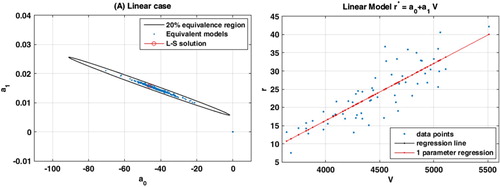
Figure 1(A) shows the plot of these sets with the ellipse of uncertainty for a relative data misfit of $\frac{{||\mathbf{\text{F}}\mathbf{\text{m}}-\mathbf{\text{y}}||}_2}{{||\mathbf{\text{y}}||}_2}\left(\mathrm{\%}\right)\le 20\mathrm{\%}.$ The error tolerance ($20\mathrm{\%}$) has been established based in the minimum misfit of the least-squares solution that has been found ($16.57\mathrm{\%}$). The main axes of this ellipse are the directions of the uncertainty of the identification problem, that correspond to the ${\mathbf{\text{v}}}_1,{\mathbf{\text{v}}}_2$ vectors of the $\mathbf{\text{V}}$ orthonormal basis set provided by the singular value decomposition of $\mathbf{\text{F}}$. Besides, as it was explained, the longer axis of uncertainty corresponds to the smallest singular value of $\mathbf{\text{F}}$. The main conclusion of this analysis is that the model parameters identified by the bootstrapping procedure (least-squares of random data bags) are located (or ‘sampled’) along the axis of maximum uncertainty of this linear regression problem, which is by ill-conditioned. Finally, Figure 1(B) shows the observed data, the regression line and the one-parameter regression with the simplified formulas. As it can be observed, the numerical results confirm the theoretical analysis shown above.

Figure 1. Linear regression model. (A) Ellipse of uncertainty for relative misfit of 20% and the different sets of parameters $\{a_{0k}^{LS},a_{1k}^{LS}{\}}_{k=1,\dots ,N_S}$ found in the different $N_S$ bagging experiments. The longer axis of the ellipse correspond to the direction of biggest uncertainty (smaller singular value of the system matrix). (B) Data points, regression line (black line) and one-parameter regression line. It can be observed that both lines are coincident and cannot be distinguished. This numerical result shows the accuracy provided by our theoretical analysis.

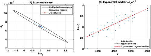
9.2. Exponential model

The linear regression line is in this case: (77) $\ln r\ast \left(V\right)=-46.37+7\times {10}^{-4}V,$(77) with a linearized relative misfit of $\frac{{||\mathbf{\text{F}}\mathbf{\text{m}}-\mathbf{\text{y}}||}_2}{{||\mathbf{\text{y}}||}_2}\left(\mathrm{\%}\right)=5.8\mathrm{\%},$ where $r$ is the strength and $V$ the ultrasonic pulse velocity. The misfit is, in this case, lower due to the logarithmic reparameterization of $r$. The corresponding nonlinear relative misfit for the least-squares model amounts 17.1%, which is close to the relative misfit of the linear model.

The eigenvalues, eigenvectors and condition number are the same that in the linear case. The equation of the axis of maximum uncertainty is: (78) $a_1={10}^{-4}\left(6.96-2.22\ln a_0\right).$(78) The process of building the simulations to calculate different sets of least-squares parameters $\{\ln a_{0k}^{LS},a_{1k}^{LS}{\}}_{k=1,\dots ,N_S}$ is the same as in the linear case.

Figure 2(A) shows the plot of these sets with the ellipse of uncertainty for a nonlinear relative data misfit of $\frac{{||\mathbf{\text{F}}\left(\mathbf{\text{m}}\right)-\mathbf{\text{y}}||}_2}{{||\mathbf{\text{y}}||}_2}\left(\mathrm{\%}\right)\le 20\mathrm{\%}$. Figure 2(B) shows the observed data, the regression line and the one-parameter regression line, that has been deduced based on theoretical developments.

Figure 2. Exponential regression model: (A) Ellipse of uncertainty for relative misfit of 6% and the different sets of parameters $\{a_{0k}^{LS},a_{1k}^{LS}{\}}_{k=1,\dots ,N_S}$ found in the different $N_S$ bagging experiments. The same considerations as in the previous case for the ellipse of uncertainty apply. (B) Data points, regression line (black line) and one-parameter regression line. It can be observed that both lines are coincident and cannot be distinguished.

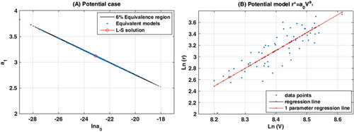
9.3. Potential model

The linear regression line is in this case: (79) $\ln r\ast \left(V\right)=-23.11+3.12\ln V,$(79) with a relative misfit of $\frac{{||\mathbf{\text{F}}\mathbf{\text{m}}-\mathbf{\text{y}}||}_2}{{||\mathbf{\text{y}}||}_2}\left(\mathrm{\%}\right)=5.76\mathrm{\%},$ where $\ln r$ and $\ln V$ are the natural logarithms of the strength and the ultrasonic pulse velocity, respectively. The corresponding nonlinear relative misfit for the least-squares model was 16.8%.

Besides, the eigenvalues, eigenvectors and condition number of the ${\mathbf{\text{F}}}^{\mathrm{T}}\mathbf{\text{F}}$ matrix are in this case: (80) $\begin{array}{rl}{\lambda }_1& =4.3\times {10}^3,{\lambda }_2=0.0073,\kappa =\sqrt{\frac{{\lambda }_1}{{\lambda }_2}}=769.34,\\ {\mathbf{\text{v}}}_1& =\left(5.04\times {10}^2,4.23\times {10}^3\right),\\ {\mathbf{\text{v}}}_2& =\left(5.04\times {10}^2,-5.99\times {10}^{-1}\right).\end{array}$(80) The equation of the axis of maximum uncertainty is in this case: (81) $a_1=0.37-0.12\ln a_0.$(81) The process to build the simulations to calculate different sets of least-squares parameters $\{\ln a_{0k}^{LS},a_{1k}^{LS}{\}}_{k=1,\dots ,N_S}$ is the same that in the previous cases.

Figure 3(A) shows the plot of these sets with the ellipse of uncertainty for a relative data misfit of $\frac{{||\mathbf{\text{F}}\mathbf{\text{m}}-\mathbf{\text{y}}||}_2}{{||\mathbf{\text{y}}||}_2}\left(\mathrm{\%}\right)\le 20\mathrm{\%}.$ Figure 3(B) shows the observed data, the regression line and the one-parameter regression line that has been deduced based on theoretical developments.

Figure 3. Potential case. (A) Ellipse of uncertainty for relative misfit of 6% and the different sets of parameters $\{a_{0k}^{LS},a_{1k}^{LS}{\}}_{k=1,\dots ,N_S}$ found in the different $N_S$ bagging experiments. The same considerations as in the previous case for the ellipse of uncertainty apply. (B) Data points, regression line (black line) and one-parameter regression line. It can be observed that both lines are coincident and cannot be distinguished.

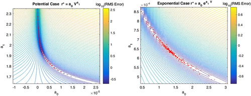
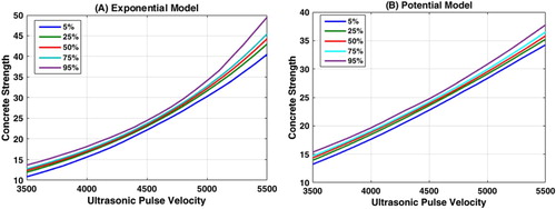
Besides, in the case of the nonlinear models (exponential and potential), the bootstrapping procedure could be also applied to the original nonlinear identification problems by solving for each data bag the corresponding nonlinear least-squares problem. In this case, instead of sampling the linearized equivalence region, the procedure would sample directly the nonlinear equivalence region that exhibits a curvilinear shape [1].

Figure 4(A, B) shows the sampling of the nonlinear equivalence region for the exponential and potential cases, induced by the bootstrapping procedure. It can be observed how the parameters are located along the curvilinear valley of lower misfits. In this case, instead of solving the linearized systems, the algorithm solves iteratively the corresponding nonlinear systems via nonlinear least-squares.

Figure 4. Potential and exponential cases. Bootstrapping procedure applied to the sampling of the nonlinear equivalence region.

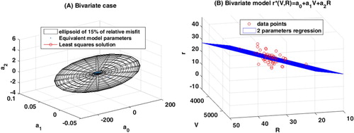
9.4. Bivariate model

The linear regression plane is: (82) $r\ast \left(V,R\right)=-44.365+0.0104V+0.709R,$(82) with a relative misfit of $\frac{{||\mathbf{\text{F}}\mathbf{\text{m}}-\mathbf{\text{y}}||}_2}{{||\mathbf{\text{y}}||}_2}\left(\mathrm{\%}\right)=13.8\mathrm{\%},$ where $r$ is the strength, $V$ the ultrasonic pulse velocity and $R$ the rebound. Therefore, constraining the concrete strength with the ultrasonic pulse velocity and the rebound is the regression method that provides the smallest data relative misfit.

The eigenvalues, eigenvectors and condition number of the ${\mathbf{\text{F}}}^{\mathrm{T}}\mathbf{\text{F}}$ matrix are: (83) $\begin{array}{rl}{\lambda }_1& =1.2\times {10}^9,{\lambda }_2=615.684,{\lambda }_3=0.504,\kappa =\sqrt{\frac{{\lambda }_1}{{\lambda }_3}}=4.89\times {10}^4.\\ {\mathbf{\text{v}}}_1& =\left(2\times {10}^{-4},1,6.8\times {10}^{-3}\right),\\ {\mathbf{\text{v}}}_2& =\left(2.3\times {10}^{-3},6.8\times {10}^{-3},-1\right),\\ {\mathbf{\text{v}}}_3& =\left(1,-2\times {10}^{-4},2.3\times {10}^{-3}\right).\end{array}$(83) This regression problem is also ill-conditioned. As in the previous cases we have obtained the simulations to calculate different sets of least-squares parameters $\{a_{0k}^{LS},a_{1k}^{LS},a_{2k}^{LS}{\}}_k=1,\dots ,N_S$.

Figure 5(A) shows the ellipsoid of 20% of relative misfit of this regression problem. It can be observed that the length of the main axis corresponding to ${\lambda }_1$ is much smaller than the two others, and the ellipsoide becomes ‘almost’ an ellipse in this case (flat ellipsoide). Finally, Figure 5(B) shows the regression plane and the observed data.

Figure 5. Bivariate linear model. (A) Ellipsoid of uncertainty for relative misfit of 15% and the different sets of parameters $\{a_{0k}^{LS},a_{1k}^{LS},a_{2k}^{LS}{\}}_{k=1,\dots ,N_S}$ found in the different $N_S$ bagging experiments. (B) Data points and regression plane.

In all the cases that have been analysed, it can be observed a perfect match between the numerical experiments and the theoretical results that have been obtained.

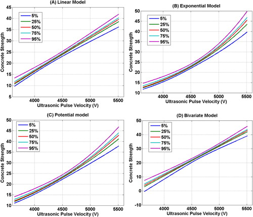
9.5. Percentile curves estimation

One of the most important achievements of the present methodology is the possibility of estimating the posterior distribution of the concrete strength for different values of the control variables: the ultrasonic pulse velocity and the rebound. For that purpose, we will be using the different sets of least-squares parameters that have been found with relative misfit lower than 20% using different data bags for each regression model. The idea consists in predicting the concrete strength for different concrete configurations in a grid of values for $\left(V,R\right)$. Based on these estimations it is possible to estimate the percentile curves for each regression model and these grids of values.

Figure 6 shows the percentile curves obtained for this data set as a function of $V$. We show the percentiles 5, 25, 50, 75 and 95 of the posterior distribution of the concrete strength estimation. This graphic works as follows: let us imagine that we have adopted the bivariate model for concrete strength estimation. Given a concrete whose ultrasonic velocity is 4800 m/s, the median strength estimation (percentile 50) is 27.98 with an interquartile range of 0.72 accounting for the uncertainty in the estimation. If the concrete velocity increases to 5400 m/s, then these numbers are: $40.70\pm 1.32$. It can be observed that in all the regression models the uncertainty is smaller for middle velocities around 4500 m/s and increases towards the extremes of the interval variation of $V$. While all the models provide a similar uncertainty quantification for middle concrete ultrasonic velocities, this confirms that nonlinear model leads to larger uncertainties. These curves can be directly used by concrete assessment experts who need to assess the risk of making a wrong assessment of local strength, since they directly include the effect of model error due to lack of fit.

Figure 6. Percentile curves for concrete strength estimation depending on the ultrasonic pulse velocity. (A) Linear model. (B) Exponential model. (C) Potential model. (D) Bivariate model (constrained with the rebound).

Finally, Figure 7 shows the percentile curves for concrete strength estimation depending on the ultrasonic pulse velocity for the exponential and potential cases. It can be observed that in the exponential case the curves are almost indistinguishable but in the potential case, they differ around 5 MPa for almost all the velocities except for 4500 m/s. In any case, we have shown that linearized or nonlinear bootstrap serve to sample the uncertainty region in these nonlinear regression models and provide a robust method to assess regression.

Figure 7. Percentile curves for concrete strength estimation depending on the ultrasonic pulse velocity deduced from the nonlinear bootstrapping sampling shown in Figure 4. (A) Exponential model. (B) Potential model. Similarities to Figures 6(B, C) can be observed.

10. Conclusions

In this paper, we have revisited the uncertainty analysis of linear regression problems through the use of linear algebra techniques, that has been inspired by the concrete strength assessment by means of non-destructive measurements. We provided an analytical expression for the direction of maximum uncertainty where the models of the linear regression problem are sampled when partial data information is used. This situation always happens in practice since data gathering is always discrete and has an economic cost. This direction of maximum uncertainty implies a trade-off between the slope and the y-intercept of the least-squares regression line. We show that using this trade-off, it is possible to write a one-parameter regression problem where the slope is the unique parameter to be identified, and its solution coincides in first approximation with the least-squares regression line. This implies that the standard regression line has the additional property of optimally taking into account the trade-off between the slope and the y-intercept of the least-squares regression line. We have also generalized this analysis to the exponential and the potential regression models and the multivariate case, with special emphasis on the bivariate case.

Finally, as a practical example, we have performed the estimation of the concrete strength by means of a non-destructive experiment (ultrasonic pulse velocity and rebound), showing the existing trade-off between the least-squares parameters for these different regression models. This fact explains why experts of NDT concrete strength estimation have identified a large variety of empirical relationships describing the same phenomenon, and opens new ways for improving the estimation of this property by sampling the posterior distribution of the regression model parameters via data bagging. We introduce the percentile curves, that provide a robust method to accomplish the concrete strength estimation and computing at the same time uncertainty, without the need of looking for the right universal regression model that does not exist. This approach generalizes the statistical results provided by ANOVA to establish critical regions using the Fisher-Snedecor statistical distribution, but in this case, only linear algebra and optimization techniques are used and serve to explain deterministically the uncertainty involved in regression problems. Besides, we have shown analytically in the case of the nonlinear regression models that nonlinear bootstrap procedure provides very similar results than the bootstrap analysis of the corresponding bootstrap systems.

Therefore, we can conclude that the novel methodology presented in this paper is a robust way of assessing the intrinsic uncertainty existing in these simple parameter identification problems, introduced by noise in data, partial knowledge about the system under research, and modelling errors. The generalization to higher dimensions is straight forward and it is currently under research.

Acknowledgements

We acknowledge Ms. Celia Fernández-Brillet for English and style corrections that served to improve the quality of this paper.

Disclosure statement

No potential conflict of interest was reported by the authors.

ORCID

Fernández-Martínez Juan Luis http://orcid.org/0000-0002-4758-2832

Fernández-Muñiz Zulima http://orcid.org/0000-0002-6544-2753

References

- Fernández-Martínez JL, Fernández-Muñiz MZ, Tompkins MJ. On the topography of the cost functional in linear and nonlinear inverse problems. Geophysics. 2012;77(1):W1–W15. doi:10.1190/geo2011-0341.1.
- Fernández-Martínez JL, Pallero JLG, Fernández-Muñiz Z, et al. From Bayes to Tarantola: new insights to understand uncertainty in inverse problems. J Appl Geophys. 2013;98:62–72. doi: 10.1016/j.jappgeo.2013.07.005
- Tarantola A, Valette B. Inverse problems = quest for information. J Geophys. 1982a;50(3):159–170.
- Tarantola A, Valette B. Generalized nonlinear inverse problems solved using the least squares criterion. Rev Geophys Space Phys. 1982b;20:219–232. doi: 10.1029/RG020i002p00219
- Scales JA, Snieder R. The anatomy of inverse problems. Geophysics. 2000;65(6):1708–1710. doi:10.1190/geo2000-0001.1.
- Scales JA, Tenorio L. Prior information and uncertainty in inverse problems. Geophysics. 2001;66(2):389–397. doi: 10.1190/1.1444930
- Biondi S. The knowledge level in existing buildings assessment. In: 14th World Conference on Earthquake Engineering; 2008 October 12–17; Beijing, China. CAEE Chinese Association. Earthquake Engineering, IAEE International Association. https://www.researchgate.net/publication/228871324_The_Knowledge_Level_in_existing_buildings_assessment
- Breysse D. Nondestructive evaluation of concrete strength: an historical review and a new perspective by combining NDT methods. Constr Build Mat. 2012;33:139–163. doi: 10.1016/j.conbuildmat.2011.12.103
- Szilagyi K, Borosnyoi A, Zsigovics I. Rebound surface hardness of concrete: introduction of an empirical constitutive model. Constr Build Mat. 2011;25:2480–2487. doi: 10.1016/j.conbuildmat.2010.11.070
- Bogas JA, Gomes MG, Gomes A. Compressive strength evaluation of structural lightweight concrete by non-destructive ultrasonic pulse velocity method. Ultrasonics. 2013;53:962–972. doi: 10.1016/j.ultras.2012.12.012
- Vasanelli E, Colangiuli D, Calia A, et al. Combining non-invasive techniques for reliable prediction of soft stone strength in historic masonries. Constr Build Mat. 2017;146:744–754. doi: 10.1016/j.conbuildmat.2017.04.146
- Breysse D, Villain G, Sbartai ZM, Garnier V. Construction of conversion models of observables into indicators, Chap. 7. In: Balayssac JP, Garnier V, editors. Non-destructive testing and evaluation of civil engineering structures. London: ISTE Press, Elsevier publication; 2018. p. 231–257.
- Qasrawi HY. Concrete strength by combined nondestructive methods simply and reliably predicted. Cem Concr Res. 2000;30:739–746. doi: 10.1016/S0008-8846(00)00226-X
- Amini K, Jalalpour M, Delatte N. Advancing concrete strength prediction using non-destructive testing: development and verification of a generalizable model. Constr Build Mat. 2016;102:762–768. doi: 10.1016/j.conbuildmat.2015.10.131
- Bashar SM, Najwa JA, Abdullahi M. Evaluation of rubbercrete based on ultrasonic pulse velocity and rebound hammer tests. Constr Build Mat. 2011;25:1388–1397. doi: 10.1016/j.conbuildmat.2010.09.004
- Nada Mahdi F, AbdMuttalib Issa S, Ali Khalid J. Prediction of compressive strength of reinforced concrete structural elements by using combined non destructive tests. J Eng. 2013;10(19):1189–1211.
- ACI 228 1R. In-place methods to estimate concrete strength. Farmington Hills (MI): American Concrete Institute; 2003.
- Alwash M, Breysse D, Sbartaï ZM. Using Monte-Carlo simulations to evaluate the efficiency of different strategies for nondestructive assessment of concrete strength. Mat Str. 2017. doi:10.1617/s11527-016-0962-x.
- Breysse D, Fernández-Martínez JL. Assessing concrete strength with rebound hammer: review of key issues and ideas for more reliable conclusions. Mater Struct. 2014;47(9):1589–1604. doi: 10.1617/s11527-013-0139-9
- Alwash M, Breysse D, Sbartaï ZM. Non-destructive strength evaluation of concrete: analysis of some key factors using synthetic simulations. Const Build Mat. 2015;99:235–245. doi: 10.1016/j.conbuildmat.2015.09.023
- Fernández-Martínez JL, Pallero JLG, Fernández-Muñiz Z, et al. The effect of noise and Tikhonov’s regularization in inverse problems. Part I: The linear case. J Appl Geophys. 2014a;108:176–185. doi:10.1016/j.jappgeo.2014.05.006.
- Fernández-Martínez JL, Pallero JLG, Fernández-Muñiz Z, et al. The effect of noise and Tikhonov’s regularization in inverse problems. Part II: the nonlinear case. J Appl Geophys. 2014b;108:186–193. doi:10.1016/j.jappgeo.2014.05.005.
- Aster C, Borchers B, Thurber CH. Parameter estimation and inverse problems. 1st ed. San Diego (CA): Elsevier Academic Press; 2005.
- Mandel J. Fitting straight lines when both variables are subject to error. J Qual Tech. 1984;16:1–14. doi: 10.1080/00224065.1984.11978881
- Cruz de Oliveira E, Fernandes de Aguiar P. Least squares regression with errors in both variables: case studies. Quim Nova. 2013;36(6):885–889. doi: 10.1590/S0100-40422013000600025
- Strang G. Linear algebra and its applications. 2nd ed. New York (NY): Academic Press; 1980.
- Oktar ON, Moral H, Tasdemir MA. Factors determining the correlations between concrete properties. Cem Concr Res. 1996;26(11):1629–1637. doi: 10.1016/S0008-8846(96)00167-6