Sensitivity analysis for the active manipulation of Helmholtz fields in 3D

Abstract

In this paper, we continue to study the feasibility of active manipulation of Helmholtz fields and by using an improved and more robust numerical strategy we present a detailed sensitivity analysis for the active methods proposed in our previous works [Onofrei D. Active manipulation of fields modelled by the Helmholtz equation. J Integral Equ. Appl. 2014;26(4):553–579; Onofrei D, Platt E. On the synthesis of acoustic sources with controllable near fields. Wave Motion. 2018;77:12–27]. In this regard, we study the behaviour of physically relevant parameters (i.e. source power, control accuracy, stability) with respect to variations in the type of control regions (bounded or unbounded), relative position of the control regions, distances between the control regions and the source, frequency range and fields to be approximated. We produce strong numerical evidence indicating the accuracy of our scheme and at the same time develop a better understanding of several important challenges for its physical implementation.

Keywords:

• Acoustic control
• inverse source problem
• field synthesis
• sensitivity analysis

1. Introduction and related results

The active control of Helmholtz fields can be studied using various techniques such as those discussed in [1–3]. Common strategies used in applications include active noise control (see early works [4–6]), sound field reproduction ([7–9] and monograph [10] with its references) and active acoustic cloaking (see [11–17] and references therein). In [18], a comprehensive comparison and analysis of the physical limitations of these approaches was done in the context of acoustic scattering.

Methods of determining active controls for acoustic cloaking based on the Green representation theorem for the Helmholtz equation were proposed in [11,19] while a construction using generalized Calderon's potentials and boundary projection operators was proposed in [20] (see also [21] where optimization of the sources of the active controls with respect to some quadratic functions of merit was performed).

In recent years many researches in the field focused their efforts on addressing the sound zone problem and its applications to personal audio systems. The goal of such efforts is to design inputs to a loud speaker array so that in a free space divided into several zones, a desired acoustic signature is synthesized in each zone, without affecting the quality of the sound produced in other zones. Among the approaches developed to solve the problem we can recall the use of the weighted pressure matching method presented in [22], energy focusing, field cancellation, and synthesis approaches compared in [23], least-squares minimization of acoustic control criteria discussed in [24] and modal-domain analysis proposed in [25] (see also [26,27], for a review on strategies for the realization of personal audio zones).

Recently, building up and extending the earlier results presented in [19], in [28,29] (see also [30] for the quasistatic case), a novel strategy was developed and discussed for the problem of controlling radiating solutions of the Helmholtz equation in two and three dimensions. More explicitly, our effort is to characterize continuous secondary surface sources for the approximation of desired Helmholtz potentials in prescribed exterior regions of space (possibly including the far field region). The sources we construct, which are modelled in our analysis as continuous boundary data, could then, for their physical implementation, be discretized in monopole or dipole arrays (see for example [31]).

In the same functional framework considered in [28,29], in [32] the authors present a sensitivity study for the problem of characterizing surface sources with vanishingly small far fields and controllable near fields with numerical simulations in [32] performed only for the two-dimensional case.

In this paper, we present a detailed sensitivity study for the problem of three-dimensional exterior control of scalar radiating Helmholtz fields explored in [28,29] by analysing the behaviour of relevant physical measures (e.g. source power, control accuracy, stability) with respect to variations in the type of control regions (bounded or unbounded), relative position of the control regions, distances between the control regions and the exterior source, frequency and fields to be approximated. We note that the problem considered can also be cast as an inverse source problem and this immediately reveals one of the major challenges we faced: the ill-posed character such problems have which was also highlighted in our previous works.

The paper is organized as follows: Section 2 provides a discussion of relevant theoretical results obtained in [28,29],while Section 3 introduces the numerical framework and optimization schemes used in the experiments. Section 4 presents the results of the sensitivity analysis for two main configurations:

1. almost non-radiating sources with controllable near fields, i.e. radiators which approximate desired Helmholtz potentials in specified near field exterior regions while keeping a very low profile beyond a given fixed radius;

2. sources approximating desired Helmholtz potentials in a collection of specified exterior compact disjoint regions of space.

Sensitivity analysis results for configuration I are presented in Section 4.1. Sensitivity analysis results for configuration II are presented in Section 4.2 for a fixed frequency and in Section 4.3 for a range of superimposed frequencies. Section 5 presents our conclusions and announces some of our future research reports on this subject.

2. Introduction of the problem

In this section, we present a general description of the scalar control problem we discuss describing the geometric and functional framework together with several essential theoretical results from [28,29].

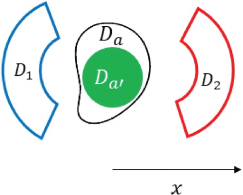
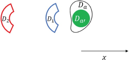
Although our results will apply for any homogeneous isotropic medium and arbitrary number of exterior control regions, for illustrative purposes we consider a free space environment containing a source $D_a\subset {\mathbb{R}}^3$ (single compact region) and only two control regions $D_1$ and $D_2$ that are mutually disjoint smooth domains. We require that the control domains and the source are mutually ‘well separated’, i.e. $(D_1\cup D_2)\cap D_a=\mathrm{\varnothing }$. Under these assumptions, in what follows we will focus on two geometric configurations, namely: (1) $\begin{array}{rl}& \left(i\right)D_1\text{ bounded},D_2\text{ bounded},\\ & \left(ii\right)D_1\text{ bounded},D_2={\mathbb{R}}^3\setminus B_R\left(\mathbf{0}\right),\end{array}$(1) where here and throughout the rest of the paper $B_R\left(\mathbf{0}\right)$ denotes the ball centred in the origin and radius R. Also, by convention, throughout the paper, we assume an $e^{-\mathrm{i}\omega t}$ time dependence of the fields.

Let $u_1$ and $u_2$ be the solutions of the Helmholtz equation in neighbourhoods of $D_1$ and $D_2$, respectively. We will sometimes refer to such functions as Helmholtz potentials. Without loss of generality, assuming the source $D_a$ is mathematically modelled as a surface input (i.e. boundary data on $\mathrm{\partial }{D}_a$) we focus on the case when one of the fields $u_1$ or $u_2$ is zero. The main goal is the characterization of boundary inputs (Neumann or Dirichlet data) on the surface of $D_a$ so that the radiating solution of the Helmholtz equation exterior to $D_a$ approximates $u_1$ in $D_1$ and $u_2$ in $D_2$. That is, assuming for exemplification that $u_2=0$, the main question is to characterize the Neumann data $v_n$ (or Dirichlet data $p_b$) on the boundary $\mathrm{\partial }{D}_a$ of $D_a$ such that (2) $\begin{array}{rl}& \mathrm{\Delta }u+k^{2}u=0\text{ in }{\mathbb{R}}^3\setminus {\overline{D}}_a,\\ & \mathrm{\nabla }u\cdot \mathbf{n}=v_n,(\text{or }u=p_b)\text{ on }\mathrm{\partial }{D}_a,\\ & \left(\hat{\mathbf{x}},\mathrm{\nabla }u\left(\mathbf{x}\right)\right)-\mathrm{i}ku\left(\mathbf{x}\right)=o\left(\frac{1}{|\mathbf{x}|}\right),\text{ as }|\mathbf{x}|\to \mathrm{\infty }\text{ uniformly for all}\hat{\mathbf{x}},\end{array}$(2) and (3) $u\approx u_1\mathrm{in}{D}_1\mathrm{and}u\approx u_2=0\mathrm{in}{D}_2,$(3) in the sense of smooth norms (e.g. $C^2$ norms), where $\mathbf{n}$ denotes the outward normal to $\mathrm{\partial }{D}_a$ and here and throughout the rest of the paper $\hat{\mathbf{x}}=\mathbf{x}/|\mathbf{x}|$ denotes the unit vector along the direction $\mathbf{x}$.

In [28], it was shown that under the assumptions and geometric configurations stated above, problem (2(2) $\begin{array}{rl}& \mathrm{\Delta }u+k^{2}u=0\text{ in }{\mathbb{R}}^3\setminus {\overline{D}}_a,\\ & \mathrm{\nabla }u\cdot \mathbf{n}=v_n,(\text{or }u=p_b)\text{ on }\mathrm{\partial }{D}_a,\\ & \left(\hat{\mathbf{x}},\mathrm{\nabla }u\left(\mathbf{x}\right)\right)-\mathrm{i}ku\left(\mathbf{x}\right)=o\left(\frac{1}{|\mathbf{x}|}\right),\text{ as }|\mathbf{x}|\to \mathrm{\infty }\text{ uniformly for all}\hat{\mathbf{x}},\end{array}$(2) ) and (3(3) $u\approx u_1\mathrm{in}{D}_1\mathrm{and}u\approx u_2=0\mathrm{in}{D}_2,$(3) ) admits a solution except for a discrete family of k values. For the rest of the paper, we will assume that k will be outside this discrete family. In this context, the existence of an infinite class of smooth functions w characterizing the desired boundary inputs was established in [28]. More explicitly, for any given smooth domain $D_{a^{\prime }}$, with $D_{a^{\prime }}⋐D_a$, defining ${\mathbf{n}}_{\mathbf{y}}$ to be the outward normal to $\mathrm{\partial }{D}_{a^{\prime }}$ at $\mathbf{y}\in D_{a^{\prime }},\rho$ to be the density of the surrounding medium, c to be the wave speed and Φ to be the free space fundamental solution of the Helmholtz equation, it was established in [28] (see also [29]) that there exists an infinity of smooth functions w such that the Neumann data $v_n$ or the Dirichlet data $p_b$ required in problem (2(2) $\begin{array}{rl}& \mathrm{\Delta }u+k^{2}u=0\text{ in }{\mathbb{R}}^3\setminus {\overline{D}}_a,\\ & \mathrm{\nabla }u\cdot \mathbf{n}=v_n,(\text{or }u=p_b)\text{ on }\mathrm{\partial }{D}_a,\\ & \left(\hat{\mathbf{x}},\mathrm{\nabla }u\left(\mathbf{x}\right)\right)-\mathrm{i}ku\left(\mathbf{x}\right)=o\left(\frac{1}{|\mathbf{x}|}\right),\text{ as }|\mathbf{x}|\to \mathrm{\infty }\text{ uniformly for all}\hat{\mathbf{x}},\end{array}$(2) – 3(3) $u\approx u_1\mathrm{in}{D}_1\mathrm{and}u\approx u_2=0\mathrm{in}{D}_2,$(3) ) are given, respectively, by (4) $\begin{array}{rl}{v}_n\left(\mathbf{x}\right)& =\frac{-i}{\rho ck}\frac{\mathrm{\partial }}{\mathrm{\partial }{\mathbf{n}}_{\mathbf{x}}}{\int }_{\mathrm{\partial }{D}_{a^{\prime }}}w\left(y\right)\frac{\mathrm{\partial \Phi }(\mathbf{x},\mathbf{y})}{\mathrm{\partial }{\mathbf{n}}_{\mathbf{y}}}\mathrm{d}{s}_{\mathbf{y}}\end{array}$(4) (5) $\begin{array}{rl}\mathrm{and}{p}_b\left(\mathbf{x}\right)& ={\int }_{\mathrm{\partial }{D}_{a^{\prime }}}w\left(y\right)\frac{\mathrm{\partial \Phi }(\mathbf{x},\mathbf{y})}{\mathrm{\partial }{\mathbf{n}}_{\mathbf{y}}}\mathrm{d}{s}_{\mathbf{y}},\end{array}$(5) for all $\mathbf{x}\in \mathrm{\partial }{D}_a$. The utility of the introduction of the fictitious source region $D_{a^{\prime }}$ is justified in the following two remarks.

Remark 1

We make the observation here that the real source on the boundary of which the desired inputs $v_n$ or $p_b$ are to be prescribed is $D_a$ while, as it can be observed, for their characterization in (4(4) $\begin{array}{rl}{v}_n\left(\mathbf{x}\right)& =\frac{-i}{\rho ck}\frac{\mathrm{\partial }}{\mathrm{\partial }{\mathbf{n}}_{\mathbf{x}}}{\int }_{\mathrm{\partial }{D}_{a^{\prime }}}w\left(y\right)\frac{\mathrm{\partial \Phi }(\mathbf{x},\mathbf{y})}{\mathrm{\partial }{\mathbf{n}}_{\mathbf{y}}}\mathrm{d}{s}_{\mathbf{y}}\end{array}$(4) ) and (5(5) $\begin{array}{rl}\mathrm{and}{p}_b\left(\mathbf{x}\right)& ={\int }_{\mathrm{\partial }{D}_{a^{\prime }}}w\left(y\right)\frac{\mathrm{\partial \Phi }(\mathbf{x},\mathbf{y})}{\mathrm{\partial }{\mathbf{n}}_{\mathbf{y}}}\mathrm{d}{s}_{\mathbf{y}},\end{array}$(5) ) a ‘fictitious’ non-physical domain $D_{a^{\prime }}$ was used. So while for simplicity and ease of computations it is assumed that $D_{a^{\prime }}$ is smooth (actually spherical in the present paper) the physical source $D_a$ can have any shape as long as it is Lipschitz, compactly embeds $D_{a^{\prime }}$, and $(D_1\cup D_2)\cap D_a=\mathrm{\varnothing }$ as mentioned above.

Remark 2

From (4(4) $\begin{array}{rl}{v}_n\left(\mathbf{x}\right)& =\frac{-i}{\rho ck}\frac{\mathrm{\partial }}{\mathrm{\partial }{\mathbf{n}}_{\mathbf{x}}}{\int }_{\mathrm{\partial }{D}_{a^{\prime }}}w\left(y\right)\frac{\mathrm{\partial \Phi }(\mathbf{x},\mathbf{y})}{\mathrm{\partial }{\mathbf{n}}_{\mathbf{y}}}\mathrm{d}{s}_{\mathbf{y}}\end{array}$(4) ) and (5(5) $\begin{array}{rl}\mathrm{and}{p}_b\left(\mathbf{x}\right)& ={\int }_{\mathrm{\partial }{D}_{a^{\prime }}}w\left(y\right)\frac{\mathrm{\partial \Phi }(\mathbf{x},\mathbf{y})}{\mathrm{\partial }{\mathbf{n}}_{\mathbf{y}}}\mathrm{d}{s}_{\mathbf{y}},\end{array}$(5) ), the smoothness of $D_{a^{\prime }}$ together with the fact that $D_{a^{\prime }}⋐D_a$ (where here ⋐ denotes compact embedding) implies the smoothness of the boundary inputs $v_n$ and $p_b$ on $\mathrm{\partial }{D}_a$. This makes the minimal assumption that $\mathrm{\partial }{D}_a$ is Lipschitz sufficient for the exterior problem to be well-posed.

The next remark highlights the versatility of our strategy with regards to the type of field propagator employed.

Remark 3

The boundary inputs given in (4(4) $\begin{array}{rl}{v}_n\left(\mathbf{x}\right)& =\frac{-i}{\rho ck}\frac{\mathrm{\partial }}{\mathrm{\partial }{\mathbf{n}}_{\mathbf{x}}}{\int }_{\mathrm{\partial }{D}_{a^{\prime }}}w\left(y\right)\frac{\mathrm{\partial \Phi }(\mathbf{x},\mathbf{y})}{\mathrm{\partial }{\mathbf{n}}_{\mathbf{y}}}\mathrm{d}{s}_{\mathbf{y}}\end{array}$(4) ) and (5(5) $\begin{array}{rl}\mathrm{and}{p}_b\left(\mathbf{x}\right)& ={\int }_{\mathrm{\partial }{D}_{a^{\prime }}}w\left(y\right)\frac{\mathrm{\partial \Phi }(\mathbf{x},\mathbf{y})}{\mathrm{\partial }{\mathbf{n}}_{\mathbf{y}}}\mathrm{d}{s}_{\mathbf{y}},\end{array}$(5) ) generate a solution u of (2(2) $\begin{array}{rl}& \mathrm{\Delta }u+k^{2}u=0\text{ in }{\mathbb{R}}^3\setminus {\overline{D}}_a,\\ & \mathrm{\nabla }u\cdot \mathbf{n}=v_n,(\text{or }u=p_b)\text{ on }\mathrm{\partial }{D}_a,\\ & \left(\hat{\mathbf{x}},\mathrm{\nabla }u\left(\mathbf{x}\right)\right)-\mathrm{i}ku\left(\mathbf{x}\right)=o\left(\frac{1}{|\mathbf{x}|}\right),\text{ as }|\mathbf{x}|\to \mathrm{\infty }\text{ uniformly for all}\hat{\mathbf{x}},\end{array}$(2) – 3(3) $u\approx u_1\mathrm{in}{D}_1\mathrm{and}u\approx u_2=0\mathrm{in}{D}_2,$(3) ) as a double layer potential given by (6) $u\left(\mathbf{x}\right)={\int }_{\mathrm{\partial }{D}_{a^{\prime }}}w\left(y\right)\frac{\mathrm{\partial \Phi }(\mathbf{x},\mathbf{y})}{\mathrm{\partial }{\mathbf{n}}_{\mathbf{y}}}\mathrm{d}{s}_{\mathbf{y}},$(6) for all $\mathbf{x}\in {\mathbb{R}}^3\setminus {\overline{D}}_a$. On the other hand, as described in [29], our analysis permits the characterization of solutions u of (2(2) $\begin{array}{rl}& \mathrm{\Delta }u+k^{2}u=0\text{ in }{\mathbb{R}}^3\setminus {\overline{D}}_a,\\ & \mathrm{\nabla }u\cdot \mathbf{n}=v_n,(\text{or }u=p_b)\text{ on }\mathrm{\partial }{D}_a,\\ & \left(\hat{\mathbf{x}},\mathrm{\nabla }u\left(\mathbf{x}\right)\right)-\mathrm{i}ku\left(\mathbf{x}\right)=o\left(\frac{1}{|\mathbf{x}|}\right),\text{ as }|\mathbf{x}|\to \mathrm{\infty }\text{ uniformly for all}\hat{\mathbf{x}},\end{array}$(2) – 3(3) $u\approx u_1\mathrm{in}{D}_1\mathrm{and}u\approx u_2=0\mathrm{in}{D}_2,$(3) ) that are complex linear combinations of single and double layer potentials. This form is efficient when dealing with real wave numbers k.

3. Numerical framework and optimization scheme

In this section, we briefly present the numerical framework and optimization scheme we employ in the study of the problems (2(2) $\begin{array}{rl}& \mathrm{\Delta }u+k^{2}u=0\text{ in }{\mathbb{R}}^3\setminus {\overline{D}}_a,\\ & \mathrm{\nabla }u\cdot \mathbf{n}=v_n,(\text{or }u=p_b)\text{ on }\mathrm{\partial }{D}_a,\\ & \left(\hat{\mathbf{x}},\mathrm{\nabla }u\left(\mathbf{x}\right)\right)-\mathrm{i}ku\left(\mathbf{x}\right)=o\left(\frac{1}{|\mathbf{x}|}\right),\text{ as }|\mathbf{x}|\to \mathrm{\infty }\text{ uniformly for all}\hat{\mathbf{x}},\end{array}$(2) –3(3) $u\approx u_1\mathrm{in}{D}_1\mathrm{and}u\approx u_2=0\mathrm{in}{D}_2,$(3) ). We also describe the set-up and parameters used in the numerical simulations. The sensitivity analysis performed later in the paper is based on the optimization scheme described below.

In [32], the $L^2$-optimization and sensitivity analysis for the solutions of the two-dimensional analogue of (2(2) $\begin{array}{rl}& \mathrm{\Delta }u+k^{2}u=0\text{ in }{\mathbb{R}}^3\setminus {\overline{D}}_a,\\ & \mathrm{\nabla }u\cdot \mathbf{n}=v_n,(\text{or }u=p_b)\text{ on }\mathrm{\partial }{D}_a,\\ & \left(\hat{\mathbf{x}},\mathrm{\nabla }u\left(\mathbf{x}\right)\right)-\mathrm{i}ku\left(\mathbf{x}\right)=o\left(\frac{1}{|\mathbf{x}|}\right),\text{ as }|\mathbf{x}|\to \mathrm{\infty }\text{ uniformly for all}\hat{\mathbf{x}},\end{array}$(2) –3(3) $u\approx u_1\mathrm{in}{D}_1\mathrm{and}u\approx u_2=0\mathrm{in}{D}_2,$(3) ) in the case of geometry (1(1) $\begin{array}{rl}& \left(i\right)D_1\text{ bounded},D_2\text{ bounded},\\ & \left(ii\right)D_1\text{ bounded},D_2={\mathbb{R}}^3\setminus B_R\left(\mathbf{0}\right),\end{array}$(1) –ii) showed that a good approximation for a stable solution with minimal power budget is achieved when $D_1$ is very near to $D_a$. Meanwhile, the three-dimensional formulation was solved using the Tikhonov regularization with the Morozov discrepancy principle. Results from [28,32] show that in order to find approximate smooth controls in $D_1$ and $D_2$, it suffices to have $L^2$ controls on the boundaries of slightly larger sets $W_1$ and $W_2$ with $D_1⋐W_1,D_2⋐W_2,W_1\cap W_2=\mathrm{\varnothing }$ and $(W_1\cup W_2)\cap D_a=\mathrm{\varnothing }$. In this regard, solution u can be approximated by the following ansatz: (7) $\mathcal{D}\left(w_{\alpha }\right)\left(\mathbf{x}\right)={\eta }_1{\int }_{\mathrm{\partial }{D}_{a^{\prime }}}{w}_{\alpha }\left(\mathbf{y}\right)\frac{\mathrm{\partial \Phi }(\mathbf{x},\mathbf{y})}{\mathrm{\partial }{\mathbf{n}}_{\mathbf{y}}}\mathrm{d}{S}_{\mathbf{y}}+\mathrm{i}{\eta }_2{\int }_{\mathrm{\partial }{D}_{a^{\prime }}}{w}_{\alpha }\left(\mathbf{y}\right)\mathrm{\Phi }(\mathbf{x},\mathbf{y})\mathrm{d}{S}_{\mathbf{y}},$(7) where ${\eta }_1,{\eta }_2\in \mathbb{R}$ are fixed parameters indicating the weight assigned to the double- and single-layer potential terms. The function $w_{\alpha }$ is the Tikhonov regularization solution, i.e. the minimizer of the discrepancy functional, (8) $F\left(w\right)=\frac{1}{\parallel w{\parallel }_{L^2\left(\mathrm{\partial }{D}_a\right)}^2}\parallel \mathcal{D}\left(w\right)-u_1{\parallel }_{L^2\left(\mathrm{\partial }{W}_1\right)}^2+\mu \parallel \mathcal{D}\left(w\right){\parallel }_{L^2\left(\mathrm{\partial }{W}_2\right)}^2+\alpha \parallel w{\parallel }_{L^2\left(\mathrm{\partial }{D}_{a^{\prime }}\right)}^2,$(8) with the regularization parameter α (computed following the Morozov Discrepancy principle) representing the penalty weight for the power required by the solution and with the weight μ given by (9) $\mu =\left\{\begin{array}{ll}1,& \text{ if }{D}_2\text{ is bounded },\\ \frac{1}{4\pi R^2},& \text{ if }{D}_2={\mathbb{R}}^3\setminus B_R\left(\mathbf{0}\right),\end{array}\right.$(9) where, here and further in the paper, $B_R\left(\mathbf{0}\right)$ denotes the ball centred on the origin with a large enough radius R such that $D_a\cup W_1⋐B_R\left(\mathbf{0}\right)$.

Numerical simulations for the synthesis of the prescribed patterns on the regions $D_1$ and $D_2$ are performed using the spherical harmonics decomposition of $w_{\alpha }$ with L harmonic orders, i.e. (10) $w_{\alpha }\left(\mathbf{y}\right)=\sum _{l=0}^L\sum _{p=-l}^l{\alpha }_{pl}{Y}_l^p\left(\hat{\mathbf{y}}\right),\text{for }\mathbf{y}\in \mathrm{\partial }{D}_{a^{\prime }},$(10) for different prescribed values of L, where $Y_l^p$ above form the orthonormal family of spherical harmonics as considered in [33, Chapter 2], [34]. For illustrative purposes, we assumed in the numerics that the fictitious source , i.e. $D_{a^{\prime }}$ above, is a single sphere $B_{a^{\prime }}\left(\mathbf{0}\right)$ with $a^{\prime }=0.01\mathrm{m}$ discretized into 20, 000 points with 200 by 100 equidistant azimuthal and polar increments, respectively. Unless stated otherwise, for the initial geometries described in (1(1) $\begin{array}{rl}& \left(i\right)D_1\text{ bounded},D_2\text{ bounded},\\ & \left(ii\right)D_1\text{ bounded},D_2={\mathbb{R}}^3\setminus B_R\left(\mathbf{0}\right),\end{array}$(1) ), the near field or primary control region $D_1$ is defined as: (11) $D_1=\left\{(r,\theta ,\phi ):r\in [0.011,0.015],\theta \in \left[-\frac{\pi }{4},\frac{\pi }{4}\right],\phi \in \left[\frac{3\pi }{4},\frac{5\pi }{4}\right]\right\},$(11) and, for configuration described at (1(1) $\begin{array}{rl}& \left(i\right)D_1\text{ bounded},D_2\text{ bounded},\\ & \left(ii\right)D_1\text{ bounded},D_2={\mathbb{R}}^3\setminus B_R\left(\mathbf{0}\right),\end{array}$(1) –i), $D_2$ is a secondary bounded control region defined by (12) $\begin{array}{rl}{D}_2& =\left\{(r,\theta ,\phi ):r\in [0.011,0.015],\theta \in \left[-\frac{\pi }{4},\frac{\pi }{4}\right],\right.\\ & \left.\phi \in \left[\frac{7\pi }{4},2\pi \right]\cup \left[0,\frac{\pi }{4}\right]\right\}+(0.09,0,0),\end{array}$(12) while for the configuration introduced at (1(1) $\begin{array}{rl}& \left(i\right)D_1\text{ bounded},D_2\text{ bounded},\\ & \left(ii\right)D_1\text{ bounded},D_2={\mathbb{R}}^3\setminus B_R\left(\mathbf{0}\right),\end{array}$(1) –ii) it is given by, (13) $D_2={\mathbb{R}}^3\setminus B_{10}\left(\mathbf{0}\right).$(13) In [29], the method of moments together with the Tikhonov regularization procedure with Morozov discrepancy principle were used towards a solution for the above problems. Specialized Gauss–Legendre quadrature procedures were employed to numerically compute the moments represented by $\mathcal{D}\left(Y_l^p\right)$, where $\mathcal{D}$ is the integral operator propagator defined at (7(7) $\mathcal{D}\left(w_{\alpha }\right)\left(\mathbf{x}\right)={\eta }_1{\int }_{\mathrm{\partial }{D}_{a^{\prime }}}{w}_{\alpha }\left(\mathbf{y}\right)\frac{\mathrm{\partial \Phi }(\mathbf{x},\mathbf{y})}{\mathrm{\partial }{\mathbf{n}}_{\mathbf{y}}}\mathrm{d}{S}_{\mathbf{y}}+\mathrm{i}{\eta }_2{\int }_{\mathrm{\partial }{D}_{a^{\prime }}}{w}_{\alpha }\left(\mathbf{y}\right)\mathrm{\Phi }(\mathbf{x},\mathbf{y})\mathrm{d}{S}_{\mathbf{y}},$(7) ). This strategy proved to be very sensitive near the source and cost inefficient when attempting to use more harmonic orders in the description of the density function $w_{\alpha }$ or perform a time domain simulation through related Fourier synthesis.

For the current research effort we developed a more direct approach where the moments $\mathcal{D}\left(Y_l^p\right)$ (with $\mathcal{D}$ defined at (7(7) $\mathcal{D}\left(w_{\alpha }\right)\left(\mathbf{x}\right)={\eta }_1{\int }_{\mathrm{\partial }{D}_{a^{\prime }}}{w}_{\alpha }\left(\mathbf{y}\right)\frac{\mathrm{\partial \Phi }(\mathbf{x},\mathbf{y})}{\mathrm{\partial }{\mathbf{n}}_{\mathbf{y}}}\mathrm{d}{S}_{\mathbf{y}}+\mathrm{i}{\eta }_2{\int }_{\mathrm{\partial }{D}_{a^{\prime }}}{w}_{\alpha }\left(\mathbf{y}\right)\mathrm{\Phi }(\mathbf{x},\mathbf{y})\mathrm{d}{S}_{\mathbf{y}},$(7) )) are evaluated explicitly by employing a truncated series obtained by making use of the addition theorem for the representation of the fundamental solution $\mathrm{\Phi }(\mathbf{x},\mathbf{y})$. More explicitly, from the addition theorem [33, Chapter 2] we have (14) $\mathrm{\Phi }(\mathbf{x},\mathbf{y})=\mathrm{i}k\sum _{n=0}^{\mathrm{\infty }}\sum _{m=-n}^n{h}_n^{\left(1\right)}\left(k|\mathbf{x}|\right)Y_n^m\left(\hat{x}\right)j_n\left(k|\mathbf{y}|\right)\overline{Y_n^m\left(\hat{y}\right)},$(14) where $h_n^{\left(1\right)},j_n$ are the spherical Haenkel of the first kind and spherical Bessel functions of order n ([33, Chapter 2], see also [34,35]) and where $Y_n^m$ form the orthonormal family as above in (10(10) $w_{\alpha }\left(\mathbf{y}\right)=\sum _{l=0}^L\sum _{p=-l}^l{\alpha }_{pl}{Y}_l^p\left(\hat{\mathbf{y}}\right),\text{for }\mathbf{y}\in \mathrm{\partial }{D}_{a^{\prime }},$(10) ). Then, considering the expansion for $w_{\alpha }$ defined in (10(10) $w_{\alpha }\left(\mathbf{y}\right)=\sum _{l=0}^L\sum _{p=-l}^l{\alpha }_{pl}{Y}_l^p\left(\hat{\mathbf{y}}\right),\text{for }\mathbf{y}\in \mathrm{\partial }{D}_{a^{\prime }},$(10) ) together with (14(14) $\mathrm{\Phi }(\mathbf{x},\mathbf{y})=\mathrm{i}k\sum _{n=0}^{\mathrm{\infty }}\sum _{m=-n}^n{h}_n^{\left(1\right)}\left(k|\mathbf{x}|\right)Y_n^m\left(\hat{x}\right)j_n\left(k|\mathbf{y}|\right)\overline{Y_n^m\left(\hat{y}\right)},$(14) ) and orthogonality of the spherical harmonics, we obtain (15) $\begin{array}{rl}{\int }_{\mathrm{\partial }{D}_{a^{\prime }}}{w}_{\alpha }\left(\mathbf{y}\right)\frac{\mathrm{\partial \Phi }(\mathbf{x},\mathbf{y})}{\mathrm{\partial }{\mathbf{n}}_{\mathbf{y}}}\mathrm{d}{s}_{\mathbf{y}}& =\mathrm{i}{k}^2{a^{\prime }}^2\sum _{l=0}^L\sum _{p=-l}^l{\alpha }_{pl}{j}_l^{\prime }k\left(|\mathbf{x}|\right)h_l^{\left(1\right)}\left(k|\mathbf{x}|\right)Y_l^p\left(\hat{\mathbf{x}}\right),\end{array}$(15) (16) $\begin{array}{rl}{\int }_{\mathrm{\partial }{D}_{a^{\prime }}}{w}_{\alpha }\left(\mathbf{y}\right)\mathrm{\Phi }(\mathbf{x},\mathbf{y})\mathrm{d}{s}_{\mathbf{y}}& =\mathrm{i}k{a^{\prime }}^2\sum _{l=0}^L\sum _{p=-l}^l{\alpha }_{pl}{j}_l\left(k|\mathbf{x}|\right)h_l^{\left(1\right)}\left(k|\mathbf{x}|\right)Y_l^p\left(\hat{\mathbf{x}}\right).\end{array}$(16) Expressions (15(15) $\begin{array}{rl}{\int }_{\mathrm{\partial }{D}_{a^{\prime }}}{w}_{\alpha }\left(\mathbf{y}\right)\frac{\mathrm{\partial \Phi }(\mathbf{x},\mathbf{y})}{\mathrm{\partial }{\mathbf{n}}_{\mathbf{y}}}\mathrm{d}{s}_{\mathbf{y}}& =\mathrm{i}{k}^2{a^{\prime }}^2\sum _{l=0}^L\sum _{p=-l}^l{\alpha }_{pl}{j}_l^{\prime }k\left(|\mathbf{x}|\right)h_l^{\left(1\right)}\left(k|\mathbf{x}|\right)Y_l^p\left(\hat{\mathbf{x}}\right),\end{array}$(15) ) and (16(16) $\begin{array}{rl}{\int }_{\mathrm{\partial }{D}_{a^{\prime }}}{w}_{\alpha }\left(\mathbf{y}\right)\mathrm{\Phi }(\mathbf{x},\mathbf{y})\mathrm{d}{s}_{\mathbf{y}}& =\mathrm{i}k{a^{\prime }}^2\sum _{l=0}^L\sum _{p=-l}^l{\alpha }_{pl}{j}_l\left(k|\mathbf{x}|\right)h_l^{\left(1\right)}\left(k|\mathbf{x}|\right)Y_l^p\left(\hat{\mathbf{x}}\right).\end{array}$(16) ) are then used in the regularization routine for a much faster and more accurate computational tool to perform our current sensitivity analysis.

4. Numerical results and sensitivity analysis

In this section, we present the sensitivity results obtained using the scheme discussed in the preceding sections. We consider two major geometries:

1. Sources approximating a prescribed Helmholtz potential in $D_1$ defined at (11(11) $D_1=\left\{(r,\theta ,\phi ):r\in [0.011,0.015],\theta \in \left[-\frac{\pi }{4},\frac{\pi }{4}\right],\phi \in \left[\frac{3\pi }{4},\frac{5\pi }{4}\right]\right\},$(11) ) with very low field amplitudes in $D_2={\mathbb{R}}^3\setminus B_{10}\left(\mathbf{0}\right)$ (i.e. exterior of the ball of radius 10 m).

   For the case when the source is geometrically modelled as a single compact region, we considered problem (2(2) $\begin{array}{rl}& \mathrm{\Delta }u+k^{2}u=0\text{ in }{\mathbb{R}}^3\setminus {\overline{D}}_a,\\ & \mathrm{\nabla }u\cdot \mathbf{n}=v_n,(\text{or }u=p_b)\text{ on }\mathrm{\partial }{D}_a,\\ & \left(\hat{\mathbf{x}},\mathrm{\nabla }u\left(\mathbf{x}\right)\right)-\mathrm{i}ku\left(\mathbf{x}\right)=o\left(\frac{1}{|\mathbf{x}|}\right),\text{ as }|\mathbf{x}|\to \mathrm{\infty }\text{ uniformly for all}\hat{\mathbf{x}},\end{array}$(2) ) and (3(3) $u\approx u_1\mathrm{in}{D}_1\mathrm{and}u\approx u_2=0\mathrm{in}{D}_2,$(3) ) and addressed the sensitivity of the control results with respect to the size of $D_1$ and its distance from the fictitious source $D_{a^{\prime }}$.

2. Sources approximating a prescribed Helmholtz potential in $D_1$ defined at (11(11) $D_1=\left\{(r,\theta ,\phi ):r\in [0.011,0.015],\theta \in \left[-\frac{\pi }{4},\frac{\pi }{4}\right],\phi \in \left[\frac{3\pi }{4},\frac{5\pi }{4}\right]\right\},$(11) ) and another prescribed Helmholtz potential in $D_2$ defined at (12(12) $\begin{array}{rl}{D}_2& =\left\{(r,\theta ,\phi ):r\in [0.011,0.015],\theta \in \left[-\frac{\pi }{4},\frac{\pi }{4}\right],\right.\\ & \left.\phi \in \left[\frac{7\pi }{4},2\pi \right]\cup \left[0,\frac{\pi }{4}\right]\right\}+(0.09,0,0),\end{array}$(12) ).

For this geometry, we assume the source modelled geometrically as a single compact region and for problem (2(2) $\begin{array}{rl}& \mathrm{\Delta }u+k^{2}u=0\text{ in }{\mathbb{R}}^3\setminus {\overline{D}}_a,\\ & \mathrm{\nabla }u\cdot \mathbf{n}=v_n,(\text{or }u=p_b)\text{ on }\mathrm{\partial }{D}_a,\\ & \left(\hat{\mathbf{x}},\mathrm{\nabla }u\left(\mathbf{x}\right)\right)-\mathrm{i}ku\left(\mathbf{x}\right)=o\left(\frac{1}{|\mathbf{x}|}\right),\text{ as }|\mathbf{x}|\to \mathrm{\infty }\text{ uniformly for all}\hat{\mathbf{x}},\end{array}$(2) ) and (3(3) $u\approx u_1\mathrm{in}{D}_1\mathrm{and}u\approx u_2=0\mathrm{in}{D}_2,$(3) ) we perform the sensitivity analysis of the control scheme with respect to the relative position of the two control regions $D_1$ and $D_2$. We also study the sensitivity of our control scheme when a small amplitude field is generated in the near field region $D_1$ and a plane wave is approximated in region $D_2$ (i.e. problem (2(2) $\begin{array}{rl}& \mathrm{\Delta }u+k^{2}u=0\text{ in }{\mathbb{R}}^3\setminus {\overline{D}}_a,\\ & \mathrm{\nabla }u\cdot \mathbf{n}=v_n,(\text{or }u=p_b)\text{ on }\mathrm{\partial }{D}_a,\\ & \left(\hat{\mathbf{x}},\mathrm{\nabla }u\left(\mathbf{x}\right)\right)-\mathrm{i}ku\left(\mathbf{x}\right)=o\left(\frac{1}{|\mathbf{x}|}\right),\text{ as }|\mathbf{x}|\to \mathrm{\infty }\text{ uniformly for all}\hat{\mathbf{x}},\end{array}$(2) ) and (3(3) $u\approx u_1\mathrm{in}{D}_1\mathrm{and}u\approx u_2=0\mathrm{in}{D}_2,$(3) ) with $u_1=0$). We conclude the discussion for this geometry with the sensitivity analysis with respect to frequency and simulate, through a Fourier synthesis procedure, a time domain source approximating an outgoing pulse in region $D_1$ and a null in region $D_2$.

Our sensitivity analysis will consider the behaviour of the following physically relevant quantities with respect to various specified geometrical parameters: $||w_{\alpha }|{|}_{L^2\left(\mathrm{\partial }{D}_{a^{\prime }}\right)}$ as an indicator of the overall power on the source, stability of the solution $w_{\alpha }$ (see definition (17(17) $S(w,w_{ϵ})=\frac{\parallel w_{\alpha }-w_{{\alpha }_{ϵ}}{\parallel }_{L^2\left(\mathrm{\partial }{D}_{a^{\prime }}\right)}}{\parallel w_{\alpha }{\parallel }_{L^2\left(\mathrm{\partial }{D}_{a^{\prime }}\right)}},$(17) ) below), $L^2$ and $L^{\mathrm{\infty }}$ relative error (i.e. relative difference in the respective norms) in the region where we approximate a plane wave and absolute $L^2$ and respectively $L^{\mathrm{\infty }}$ error in the null region (error computed on $\mathrm{\partial }{D}_2$ when $D_2={\mathbb{R}}^3\setminus B_{10}\left(\mathbf{0}\right)$). The stability measure is the $L^2$ relative norm of the difference of antenna density patterns: (17) $S(w,w_{ϵ})=\frac{\parallel w_{\alpha }-w_{{\alpha }_{ϵ}}{\parallel }_{L^2\left(\mathrm{\partial }{D}_{a^{\prime }}\right)}}{\parallel w_{\alpha }{\parallel }_{L^2\left(\mathrm{\partial }{D}_{a^{\prime }}\right)}},$(17) where $w_{{\alpha }_{ϵ}}$ is the solution of problem (2(2) $\begin{array}{rl}& \mathrm{\Delta }u+k^{2}u=0\text{ in }{\mathbb{R}}^3\setminus {\overline{D}}_a,\\ & \mathrm{\nabla }u\cdot \mathbf{n}=v_n,(\text{or }u=p_b)\text{ on }\mathrm{\partial }{D}_a,\\ & \left(\hat{\mathbf{x}},\mathrm{\nabla }u\left(\mathbf{x}\right)\right)-\mathrm{i}ku\left(\mathbf{x}\right)=o\left(\frac{1}{|\mathbf{x}|}\right),\text{ as }|\mathbf{x}|\to \mathrm{\infty }\text{ uniformly for all}\hat{\mathbf{x}},\end{array}$(2) ) and (3(3) $u\approx u_1\mathrm{in}{D}_1\mathrm{and}u\approx u_2=0\mathrm{in}{D}_2,$(3) ) with noise of magnitude ε in the data $u_1,u_2$. In this paper, our noise is modelled as a uniformly distributed additive perturbation of order ε.

Unless otherwise specified, each single-source sensitivity test was performed on two synthesis results: one with 15 and another with 30 harmonic orders used in (10(10) $w_{\alpha }\left(\mathbf{y}\right)=\sum _{l=0}^L\sum _{p=-l}^l{\alpha }_{pl}{Y}_l^p\left(\hat{\mathbf{y}}\right),\text{for }\mathbf{y}\in \mathrm{\partial }{D}_{a^{\prime }},$(10) ).

4.1. Almost non-radiating source with controllable near field

In the following tests, we consider a single almost non-radiating source $D_a$ containing the following fictitious region $D_{a^{\prime }}=B_{0.01}\left(\mathbf{0}\right)$, i.e. a sphere centred at the origin and with radius $1\mathrm{cm}$. We also consider the near control region $D_1$ as defined in (11(11) $D_1=\left\{(r,\theta ,\phi ):r\in [0.011,0.015],\theta \in \left[-\frac{\pi }{4},\frac{\pi }{4}\right],\phi \in \left[\frac{3\pi }{4},\frac{5\pi }{4}\right]\right\},$(11) ) where we match an incoming plane wave $u_1\left(\mathbf{x}\right)=e^{\mathrm{i}\mathbf{x}\cdot \left(10{\hat{\mathbf{e}}}_1\right)}$ propagating along the positive x-axis (i.e. towards the source $D_a$), with ${\hat{\mathbf{e}}}_1=⟨1,0,0⟩$ and the wave number k=10, and the far field region the exterior of a ball centred at the origin of radius $10m$, i.e. $D_2={\mathbb{R}}^3\setminus B_{10}\left(\mathbf{0}\right)$ given in (13), where we maintain a near zero signature, i.e. $u_2\left(\mathbf{x}\right)\approx 0$. 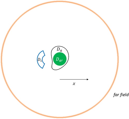This initial geometry is shown in Figure 1.

Figure 1. Initial geometry for the sensitivity experiments with an almost non-radiating single source.

We recall that as stated above and proved in [28] our method is such that only good boundary controls are needed for smooth interior controls. In this spirit, in Sections 4.1.1, 4.1.2, and 4.1.3, the boundary of region $D_1$ is uniformly discretized into 2400 points, while the far field boundary, i.e. $\mathrm{\partial }{D}_2=\mathrm{\partial }{B}_{10}\left(\mathbf{0}\right),$ is uniformly discretized with 20,000 points with 200 in the azimuthal and 100 in the polar direction, respectively.

This geometry was considered in [29] where we obtained a density $w_{\alpha }$ on $D_{a^{\prime }}$ (and also necessary boundary inputs as a consequence of (4(4) $\begin{array}{rl}{v}_n\left(\mathbf{x}\right)& =\frac{-i}{\rho ck}\frac{\mathrm{\partial }}{\mathrm{\partial }{\mathbf{n}}_{\mathbf{x}}}{\int }_{\mathrm{\partial }{D}_{a^{\prime }}}w\left(y\right)\frac{\mathrm{\partial \Phi }(\mathbf{x},\mathbf{y})}{\mathrm{\partial }{\mathbf{n}}_{\mathbf{y}}}\mathrm{d}{s}_{\mathbf{y}}\end{array}$(4) ) and (5(5) $\begin{array}{rl}\mathrm{and}{p}_b\left(\mathbf{x}\right)& ={\int }_{\mathrm{\partial }{D}_{a^{\prime }}}w\left(y\right)\frac{\mathrm{\partial \Phi }(\mathbf{x},\mathbf{y})}{\mathrm{\partial }{\mathbf{n}}_{\mathbf{y}}}\mathrm{d}{s}_{\mathbf{y}},\end{array}$(5) )) so that the relative control error in the region $D_1$ was of order $O\left({10}^{-3}\right)$ while maintaining field values of $O\left({10}^{-3}\right)$ in $D_2$. Recalling the ansatz for the propagating field described above at (6(6) $u\left(\mathbf{x}\right)={\int }_{\mathrm{\partial }{D}_{a^{\prime }}}w\left(y\right)\frac{\mathrm{\partial \Phi }(\mathbf{x},\mathbf{y})}{\mathrm{\partial }{\mathbf{n}}_{\mathbf{y}}}\mathrm{d}{s}_{\mathbf{y}},$(6) ) in [29] we produced numerical support showing the optimal density $w_{\alpha }$ in (6(6) $u\left(\mathbf{x}\right)={\int }_{\mathrm{\partial }{D}_{a^{\prime }}}w\left(y\right)\frac{\mathrm{\partial \Phi }(\mathbf{x},\mathbf{y})}{\mathrm{\partial }{\mathbf{n}}_{\mathbf{y}}}\mathrm{d}{s}_{\mathbf{y}},$(6) ) exhibiting maximum values of order $O\left({10}^5\right)$ and small and fast oscillations on the side facing $D_1$ with large and slower oscillation on the opposite side and at the poles.

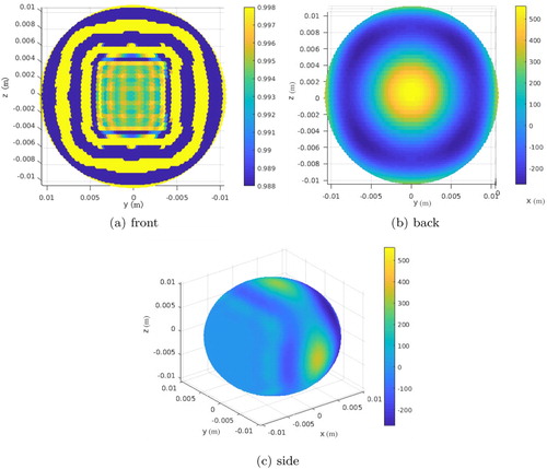
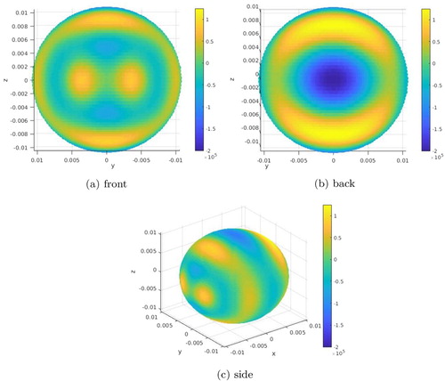
Recently, with the current updated scheme, we can accurately compute and evaluate the surface field pattern on any nearby surfaces surrounding $D_1$. Also, as suggested in Remark 1 the actual physical source boundary $\mathrm{\partial }{D}_a$ can be chosen as one needs as long as $D_a$ compactly embeds $D_{a^{\prime }}$ and $(D_1\cup D_2)\cap D_a=\mathrm{\varnothing }$. For example, in the case when the actual physical source is chosen to be the nearby sphere centred in the origin and radius a=0.015 cm, i.e. $D_a=B_{0.0105}\left(\mathbf{0}\right)$ the Dirichlet boundary input required for the desired control level is, as showed in (5(5) $\begin{array}{rl}\mathrm{and}{p}_b\left(\mathbf{x}\right)& ={\int }_{\mathrm{\partial }{D}_{a^{\prime }}}w\left(y\right)\frac{\mathrm{\partial \Phi }(\mathbf{x},\mathbf{y})}{\mathrm{\partial }{\mathbf{n}}_{\mathbf{y}}}\mathrm{d}{s}_{\mathbf{y}},\end{array}$(5) ), the restriction of the field $u\left(\mathbf{x}\right)$ described at (6(6) $u\left(\mathbf{x}\right)={\int }_{\mathrm{\partial }{D}_{a^{\prime }}}w\left(y\right)\frac{\mathrm{\partial \Phi }(\mathbf{x},\mathbf{y})}{\mathrm{\partial }{\mathbf{n}}_{\mathbf{y}}}\mathrm{d}{s}_{\mathbf{y}},$(6) ) to $\mathrm{\partial }{B}_{0.0105}\left(\mathbf{0}\right)$ and is shown in Figure 2.

Figure 2. Different views of the surface field pattern on the actual source $\mathrm{\partial }{B}_{0.0105}\left(\mathbf{0}\right)$.

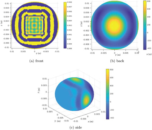
As one can observe in this picture, the surface pattern necessary on the physical source $D_a=B_{0.0105}\left(\mathbf{0}\right)$ for the desired control effect, i.e. approximation of an incoming plane wave pattern in $D_1$ with very low field values in $D_2$, exhibits a similar behaviour as was recalled above about the respective density $w_{\alpha }$ (high and fast oscillations on the side opposite to region $D_1$ (back side in the figure) with small and faster oscillations on the side facing $D_1$ (front side in the figure)). The important difference is that the required power on $\mathrm{\partial }{B}_{0.0105}\left(\mathbf{0}\right)$ would be a few orders of magnitude smaller than $||w_{\alpha }|{|}_{L^2}$ (which is $O\left({10}^5\right)$ as shown in Figure 21) and has less complexity in the pattern with a much smaller contrast in the level of oscillations throughout its surface. This is another fact which motivates us to believe that an optimal shape design for the actual source boundary could lead to a less challenging source pattern required for a good control.

4.1.1. Varying the distance of the near control

The first test of our sensitivity analysis considers the dependence of our scheme (i.e. focusing on physical quantities defined above at the beginning of Section 4) on the distance between $D_1$ and $D_{a^{\prime }}$. Two iterations of this experiment are shown in Figure 3. $D_1^{\ast }$ is the near control region after an outward shift from the antenna.

Figure 3. The near control region after an outward shift from the source.

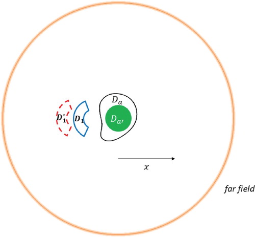
In what follows in this subsection, in each figure, the sensitivity plots are presented as a function of the distance between $D_1$ and $D_{a^{\prime }}$, first up to a distance of $0.025\mathrm{m}$ (left plot) and then going further to a distance of $0.28\mathrm{m}$ (right plot).

In Figure 4, the $L^2$ norm of the density $w_{\alpha }$ is shown as a function of the distance between $D_1$ and $D_{a^{\prime }}$. This quantity is an indication of the source power and it can be seen that it is bigger for the larger number of harmonics but in both scenarios (i.e. 15 or 30 harmonic orders) grows exponentially.

Figure 4. $L^2$ norm of the source density $w_{\alpha }$ as a function of the distance between $D_1$ and $D_{a^{\prime }}$.

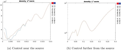
Figure 5 shows the relative supremum error in $D_1$ and Figure 6 shows the absolute supremum error on $\mathrm{\partial }{D}_2$. In Figure 7 we present our results concerning the stability of the scheme with respect to the distance between $D_1$ and $D_{a^{\prime }}$.

Figure 5. Relative supremum error in $D_1$ as a function of the distance between $D_1$ and $D_{a^{\prime }}$.

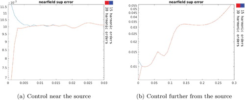
Figure 6. Absolute supremum error on $\mathrm{\partial }{D}_2$ as a function of the distance between $D_1$ and $D_{a^{\prime }}$.

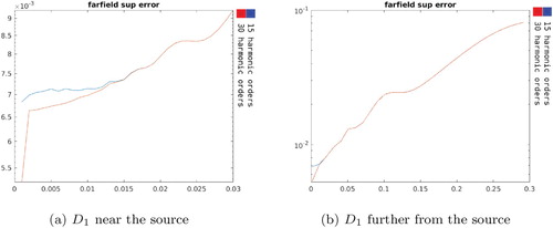
Figure 7. Stability of the scheme as a function of the distance between $D_1$ and $D_{a^{\prime }}$.

We observe that the accuracy error in $D_1$ is better in the vicinity of the source but remains of order $O\left({10}^{-2}\right)$ throughout. On the other hand, the far field absolute supremum error reaches undesirable levels when $D_1$ and $D_{a^{\prime }}$ are at distances greater than 15 cm. Overall, except the near field when more harmonic orders produce a better accuracy we observe that the number of harmonics used does not seem to make a difference in the scheme behaviour. At the same time, the stability is worse when $D_1$ is in the vicinity of the source with the observation that the scheme is more stable when less harmonic orders are used.

As a conclusion, for this sensitivity test, there seem to be a competition between accuracy and stability depending on the number of harmonics being used and the distance between $D_1$ and the fictitious source $D_{a^{\prime }}$. We mention that in applications where the field to be approximated in region $D_1$ is prescribed a priori the stability analysis may not be so relevant but what may be challenging for a practical realization is the synthesis of a radiator with the complexity suggested by our simulations. As we suggested above, based on Remark 1, in order to better address the source synthesis challenge one could employ optimization procedures for finding the best possible shape for the physical source $D_a$ or one could consider different penalty functionals in the optimization scheme.

4.1.2. Varying the outer radius of the near control

In the next test of our sensitivity analysis, we consider the behaviour of the above physically important quantities (see the beginning of Section 4) with respect to increments of the outer radius of the sectorial near control region $D_1$ described at (11(11) $D_1=\left\{(r,\theta ,\phi ):r\in [0.011,0.015],\theta \in \left[-\frac{\pi }{4},\frac{\pi }{4}\right],\phi \in \left[\frac{3\pi }{4},\frac{5\pi }{4}\right]\right\},$(11) ) while the distance between $D_1$ and the source is kept fixed.

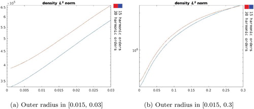
Figure 8 shows an iterate $D_1^{\ast }$ of the near control after an increase in the outer radius. Figure 9 shows the $L^2$ norm of the density $w_{\alpha }$ as a function of the increments in $D_1$ outer radius. We can observe that a larger $||w_{\alpha }|{|}_{L^2}$ is required for the 30 harmonic orders as expected. Also, since $||w_{\alpha }|{|}_{L^2}$ is an indicator of the source power, it can be seen that for larger control regions the power will tend to grow exponentially at approximately the same rate regardless of the number of harmonics used.

Figure 8. The initial near control $D_1$ and an iterate $D_1^{\ast }$ after increasing the outer radius.

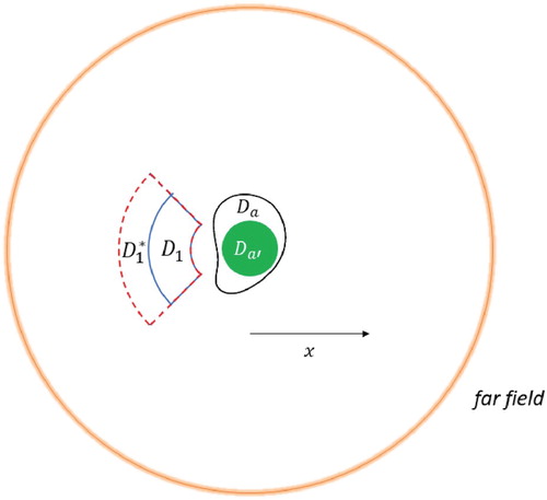
Figure 9. $L^2$ norm of the source density $w_{\alpha }$ as a function of the increments in $D_1$ outer radius.

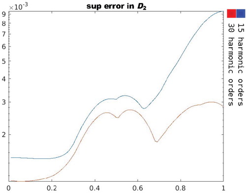
In Figures 10 and  11 one can observe that the relative supremum error in region $D_1$ and the absolute supremum error on $\mathrm{\partial }{D}_2$ are of order $O\left({10}^{-3}\right)$ in the vicinity of the source and then reach order $O\left({10}^{-2}\right)$ (outer radius approximately 2.5 cm) and grow to reach undesirable values when the region of control $D_1$ gets larger (outer radius approximatively 15 cm). This fact suggests the necessity of more harmonics to be used for greater accuracy in the context of larger control regions.

Figure 10. Relative supremum error in $D_1$ as a function of the increments in $D_1$ outer radius.

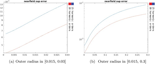
Figure 11. Absolute supremum error on $\mathrm{\partial }{D}_2$ as a function of the increments in $D_1$ outer radius.

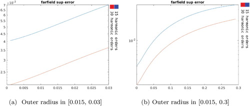
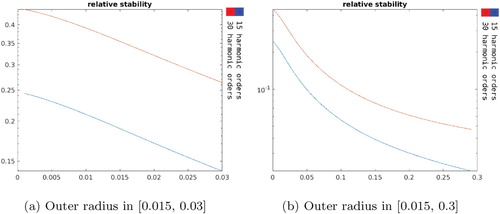
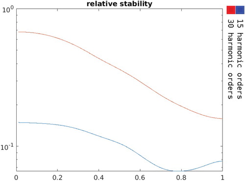
Figure 12 shows the stability getting better when region $D_1$ gets larger. Notice also that the 15 harmonic order-configuration exhibited better stability even though it is less accurate. Using higher harmonic orders remains stable while maintaining accurate results. Again, as we mentioned above, for applications where the field to be approximated in $D_1$ is a priori known the stability is not an important issue but the complexity of the source to be synthesized remains a challenge which could be mitigated as we suggested at the end of Section 4.1.1.

Figure 12. Stability measure as a function of the increments in $D_1$ outer radius.

4.1.3. Varying both the inner and outer radius of the near control

The following results show the effect of increasing both the inner and outer radius of the near control, i.e. simultaneously moving the front and back sides of the near control away from the source. The increments in both radii are always kept equal. Figure 13 illustrates two iterates $D_1$ and $D_1^{\ast }$ in this set of experiments.

Figure 13. The initial near control $D_1$ and an iterate $D_1^{\ast }$ after increasing both the inner and outer radii by equal increments.

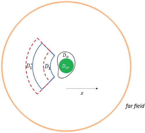
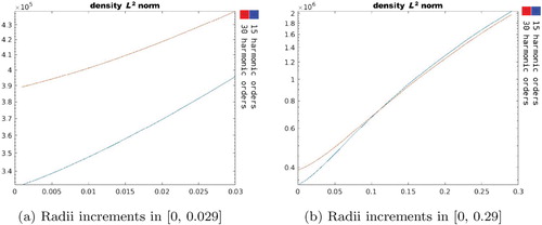
Figure 14 shows the $L^2$ norm of the density $w_{\alpha }$ as a function of the increments in both of $D_1$'s radii. As in the other cases discussed above, we observe that it grows exponentially with bigger values for more harmonics until the region is larger and further away where its value stabilizes for the two levels of harmonic orders used.

Figure 14. $L^2$ norm of the source density $w_{\alpha }$ as a function of the $D_1$ radii increment.

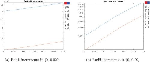
Again, the use of 15 harmonic orders produced less accurate results. In this regard, Figure 15 shows the plots of the relative supremum errors in $D_1$. The relative supremum error in $D_1$ is of order $O\left({10}^{-3}\right)$ for the first increments and remains below ${10}^{-2}$ when the radii increments are less than 10 cm reaching undesirable levels for larger radii increments. Figure 16 shows that over the entire range of increments used, the absolute supremum error in the far field stays of order $O\left({10}^{-3}\right)$ as long as the radii increments are less than 8cm and reaches order $O\left({10}^{-2}\right)$ afterwards.

Figure 15. Relative supremum error as a function of $D_1$ radii increment.

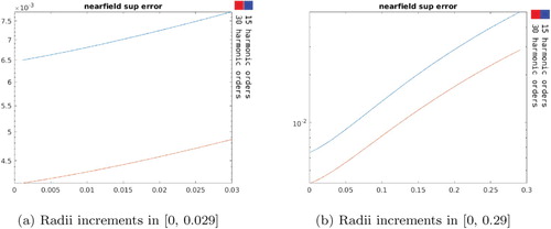
Figure 16. Absolute supremum error on $\mathrm{\partial }{D}_2$ as a function of $D_1$ radii increment.

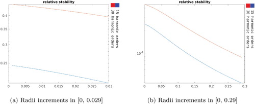
The stability measure is shown in Figure 17. Notice that as the stability gets better with larger increments in the region size and distance from the source.

Figure 17. Stability measure as a function of $D_1$ radii increment.

4.2. Multi-region controls

In the next set of tests, we consider problem (2(2) $\begin{array}{rl}& \mathrm{\Delta }u+k^{2}u=0\text{ in }{\mathbb{R}}^3\setminus {\overline{D}}_a,\\ & \mathrm{\nabla }u\cdot \mathbf{n}=v_n,(\text{or }u=p_b)\text{ on }\mathrm{\partial }{D}_a,\\ & \left(\hat{\mathbf{x}},\mathrm{\nabla }u\left(\mathbf{x}\right)\right)-\mathrm{i}ku\left(\mathbf{x}\right)=o\left(\frac{1}{|\mathbf{x}|}\right),\text{ as }|\mathbf{x}|\to \mathrm{\infty }\text{ uniformly for all}\hat{\mathbf{x}},\end{array}$(2) ) and (3(3) $u\approx u_1\mathrm{in}{D}_1\mathrm{and}u\approx u_2=0\mathrm{in}{D}_2,$(3) ) for the configuration described in (1(1) $\begin{array}{rl}& \left(i\right)D_1\text{ bounded},D_2\text{ bounded},\\ & \left(ii\right)D_1\text{ bounded},D_2={\mathbb{R}}^3\setminus B_R\left(\mathbf{0}\right),\end{array}$(1) -i) with a single fictitious source $D_{a^{\prime }}=B_{0.01}\left(\mathbf{0}\right)$ and two compact control regions $D_1$ and $D_2$ (see Figure 18).

Figure 18. The initial geometry for the multi-region controls.

For the initial geometry in our tests, the primary control region $D_1$ is defined as before (18) $D_1=\left\{(r,\theta ,\phi ):r\in [0.011,0.015],\theta \in \left[-\frac{\pi }{4},\frac{\pi }{4}\right],\phi \in \left[\frac{3\pi }{4},\frac{5\pi }{4}\right]\right\}$(18) while the secondary control region $D_2$ is given by (19) $\begin{array}{rl}{D}_2& =\left\{(r,\theta ,\phi ):r\in [0.011,0.015],\theta \in \left[-\frac{\pi }{4},\frac{\pi }{4}\right],\right.\\ & \times \left.\phi \in \left[\frac{7\pi }{4},2\pi \right]\cup \left[0,\frac{\pi }{4}\right]\right\}+(0.09,0,0).\end{array}$(19) As before, we mention that in our method only boundary controls are needed to imply smooth interior controls. The first question we address is the possibility to approximate the outgoing plane wave $u_1\left(\mathbf{x}\right)=e^{\mathrm{i}\mathbf{x}\cdot (-10{\hat{\mathbf{e}}}_1)}$ in $D_1$ while imposing a small field in $D_2$. For this problem and the subsequent sensitivity tests, the boundaries of the two regions are uniformly discretized with 2400 points each.

As in Remark 1, we recall that the actual physical source boundary is only constrained by the condition to embed the fictitious source and to have an empty intersection with $D_1\cup D_2$ and that, as it can be seen in (5(5) $\begin{array}{rl}\mathrm{and}{p}_b\left(\mathbf{x}\right)& ={\int }_{\mathrm{\partial }{D}_{a^{\prime }}}w\left(y\right)\frac{\mathrm{\partial \Phi }(\mathbf{x},\mathbf{y})}{\mathrm{\partial }{\mathbf{n}}_{\mathbf{y}}}\mathrm{d}{s}_{\mathbf{y}},\end{array}$(5) ), the required boundary input on the physical source $D_a$ will be $\mathcal{D}\left(w_{\alpha }\right)$ restricted to $\mathrm{\partial }{D}_a$. Thus, if for instance the real source $D_a$ is chosen to be the sphere $B_{0.0105}\left(\mathbf{0}\right)$ then Figure 19 shows the necessary pattern required on $\mathrm{\partial }{D}_a$ for a good control in $D_1$ and $D_2$. As observed before for the configuration (1(1) $\begin{array}{rl}& \left(i\right)D_1\text{ bounded},D_2\text{ bounded},\\ & \left(ii\right)D_1\text{ bounded},D_2={\mathbb{R}}^3\setminus B_R\left(\mathbf{0}\right),\end{array}$(1) -ii) discussed in Section 4.1, we can see in Figure 19 that the magnitude of the required boundary input on the real source $\mathrm{\partial }{B}_{0.0105}\left(\mathbf{0}\right)$ is a few orders smaller than the magnitude of the density $w_{\alpha }$ (which is $O\left({10}^5\right)$ as shown in Figure 21) and has less complexity in the pattern. This once more supports our claim that one could search and find an actual source boundary around the fictitious domain $D_{a^{\prime }}$ so that while it does not intersect $D_1\cup D_2$ it is such that the boundary input required on it needs less power for its instantiation and presents a lower level of complexity in its pattern.

Figure 19. Different views of the surface field pattern on $\mathrm{\partial }{B}_{0.0105}$.

Next we will present the sensitivity of our scheme with respect to relative positions between the two control regions. In this regard, Figure 20 shows the geometry of two iterations. In each iteration, $D_1$ is fixed while we vary the position of $D_2$ via counterclockwise rotation about $D_a$.

Figure 20. Illustration of two iterations showing the secondary region rotated around $D_a$.

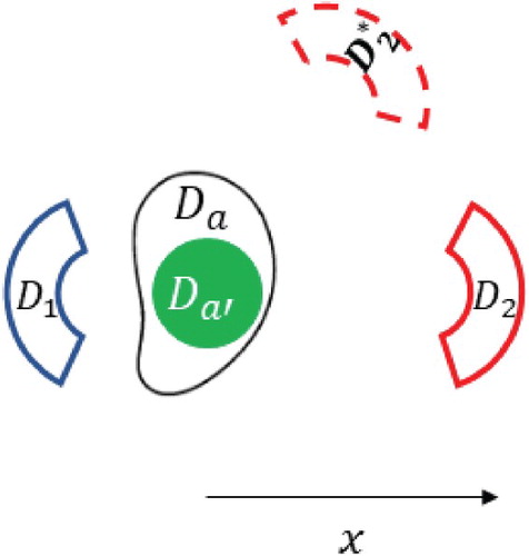
Figure 21 shows the $L^2$ norm of the density $w_{\alpha }$, as a function of the angle of rotation. We can observe that its levels remain of order $O\left({10}^6\right)$ for the entire rotation spectrum.

Figure 21. $L^2$ norm of $w_{\alpha }$ as a function of the secondary region's angle of rotation.

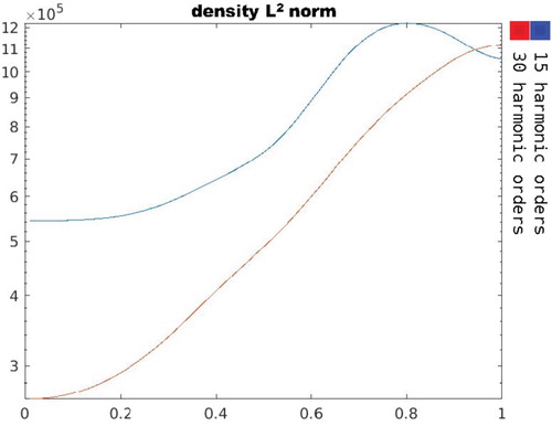
Figure 22 show the relative $L^2$ and respectively relative supremum error in region $D_1$. The performance is good with largest relative error for a 180 degree rotation but still of order $O\left({10}^{-2}\right)$.

Figure 22. Accuracy errors in $D_1$.

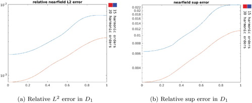
Figure 23 shows a small field generated in region $D_2$ as desired. One can see that the contrast between the field in region $D_1$ and the small field in region $D_2$ remains between approximately 40 and $60\mathrm{dB}$ with better performance for the case with more harmonic orders (where we use the $20{\log }_{10}$ convention for computing the decibel (dB) level).

Figure 23. Supremum error in $D_2$ as a function of its angle of rotation.

The stability measure is plotted in Figure 24. It tends to decrease as the angle of rotation approaches π where it is below ${10}^{-1}$.

Figure 24. Stability measure as a function of the secondary region's angle of rotation.

We continue our sensitivity analysis with another important test. That is, we study the accuracy of our scheme in the context of problem (2(2) $\begin{array}{rl}& \mathrm{\Delta }u+k^{2}u=0\text{ in }{\mathbb{R}}^3\setminus {\overline{D}}_a,\\ & \mathrm{\nabla }u\cdot \mathbf{n}=v_n,(\text{or }u=p_b)\text{ on }\mathrm{\partial }{D}_a,\\ & \left(\hat{\mathbf{x}},\mathrm{\nabla }u\left(\mathbf{x}\right)\right)-\mathrm{i}ku\left(\mathbf{x}\right)=o\left(\frac{1}{|\mathbf{x}|}\right),\text{ as }|\mathbf{x}|\to \mathrm{\infty }\text{ uniformly for all}\hat{\mathbf{x}},\end{array}$(2) ) and (3(3) $u\approx u_1\mathrm{in}{D}_1\mathrm{and}u\approx u_2=0\mathrm{in}{D}_2,$(3) ) for the same configuration described at (1(1) $\begin{array}{rl}& \left(i\right)D_1\text{ bounded},D_2\text{ bounded},\\ & \left(ii\right)D_1\text{ bounded},D_2={\mathbb{R}}^3\setminus B_R\left(\mathbf{0}\right),\end{array}$(1) -i) with one fictitious source $D_{a^{\prime }}=B_{0.01}\left(\mathbf{0}\right)$ and two compact control regions $D_1$ and $D_2$ described below and sketched in Figure 25, (20) $D_1=\left\{(r,\theta ,\phi ):r\in [0.011,0.015],\theta \in \left[-\frac{\pi }{8},\frac{\pi }{8}\right],\phi \in \left[\frac{3\pi }{4},\frac{5\pi }{4}\right]\right\}+(-0.03,0,0)$(20) and (21) $\begin{array}{r}{D}_2=\left\{(r,\theta ,\phi ):r\in [0.011,0.015],\theta \in \left[-\frac{\pi }{8},\frac{\pi }{8}\right],\phi \in \left[\frac{3\pi }{4},\frac{5\pi }{4}\right]\right\}+(-0.1,0,0).\end{array}$(21)

Figure 25. Sketch of the geometry where $D_1$ is acting as a near field obstacle to $D_2$.

The novelty of the test consist in the fact that now we consider $u_1=0$ and $u_2\left(\mathbf{x}\right)=e^{\mathrm{i}\mathbf{x}\cdot (-10{\hat{\mathbf{e}}}_1)}$ in problem (2(2) $\begin{array}{rl}& \mathrm{\Delta }u+k^{2}u=0\text{ in }{\mathbb{R}}^3\setminus {\overline{D}}_a,\\ & \mathrm{\nabla }u\cdot \mathbf{n}=v_n,(\text{or }u=p_b)\text{ on }\mathrm{\partial }{D}_a,\\ & \left(\hat{\mathbf{x}},\mathrm{\nabla }u\left(\mathbf{x}\right)\right)-\mathrm{i}ku\left(\mathbf{x}\right)=o\left(\frac{1}{|\mathbf{x}|}\right),\text{ as }|\mathbf{x}|\to \mathrm{\infty }\text{ uniformly for all}\hat{\mathbf{x}},\end{array}$(2) ) and (3(3) $u\approx u_1\mathrm{in}{D}_1\mathrm{and}u\approx u_2=0\mathrm{in}{D}_2,$(3) ), i.e. we approximate an outgoing plane wave in region $D_2$ while having a very small field in the near field region $D_1$. This geometry is relevant for applications where the objective is to focus energy or communicate behind a near field obstacle. For this simulation, we used 2400 control points on $\mathrm{\partial }{D}_1$ and 38,400 control points on $\mathrm{\partial }{D}_2$.

The overall performance of our scheme is shown in Figure 26. We can see the accuracy of the control in region $D_1$ with relative supremum error of order $O\left({10}^{-2}\right)$ and with small fields in region $D_2$ as desired. The contrast between the quiet region $D_2$ and the other control region $D_1$ is in this case over $40\mathrm{dB}$. Our numerics suggest that more harmonics and more control points in the two control regions can allow us to extend these results to the situation when region $D_2$ is larger and when region $D_1$ is much closer to the source.

Figure 26. Performance of the scheme in generating a null in $D_1$ and a plane wave in $D_2$.

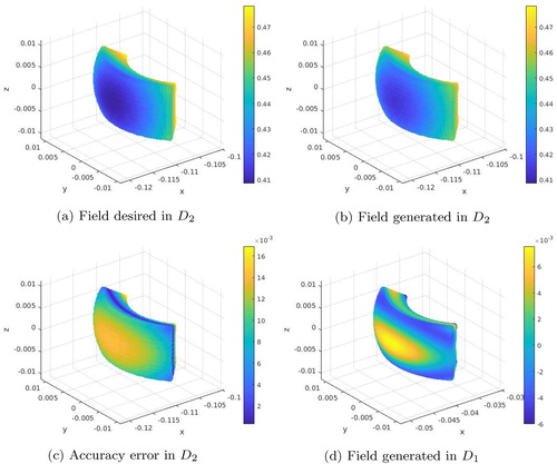
Figure 27 presents the required pattern on the actual source $D_a$ in the particular example when $D_a=B_{0.0105}\left(\mathbf{0}\right)$. The front picture refers to the part of the surface facing the control regions, the back picture shows the opposite part of the surface and the side plot presents a panoramic view of the surface pattern. We can see that the required surface pattern is much simpler and without a large variation in the field oscillation as it was the case for the geometry (1(1) $\begin{array}{rl}& \left(i\right)D_1\text{ bounded},D_2\text{ bounded},\\ & \left(ii\right)D_1\text{ bounded},D_2={\mathbb{R}}^3\setminus B_R\left(\mathbf{0}\right),\end{array}$(1) -ii) considered in Section 4.1.

Figure 27. Different views of the surface field pattern on $\mathrm{\partial }{B}_{0.0105}\left(\mathbf{0}\right)$.

Based on the previous analysis, by superposition, we could in principle predict a good accuracy for our scheme for the case of approximating multiple prescribed Helmholtz potentials in given mutually disjoint exterior regions.

4.3. Fourier synthesis

In this section, we consider again problem (2(2) $\begin{array}{rl}& \mathrm{\Delta }u+k^{2}u=0\text{ in }{\mathbb{R}}^3\setminus {\overline{D}}_a,\\ & \mathrm{\nabla }u\cdot \mathbf{n}=v_n,(\text{or }u=p_b)\text{ on }\mathrm{\partial }{D}_a,\\ & \left(\hat{\mathbf{x}},\mathrm{\nabla }u\left(\mathbf{x}\right)\right)-\mathrm{i}ku\left(\mathbf{x}\right)=o\left(\frac{1}{|\mathbf{x}|}\right),\text{ as }|\mathbf{x}|\to \mathrm{\infty }\text{ uniformly for all}\hat{\mathbf{x}},\end{array}$(2) ) and (3(3) $u\approx u_1\mathrm{in}{D}_1\mathrm{and}u\approx u_2=0\mathrm{in}{D}_2,$(3) ) for the configuration described in (1(1) $\begin{array}{rl}& \left(i\right)D_1\text{ bounded},D_2\text{ bounded},\\ & \left(ii\right)D_1\text{ bounded},D_2={\mathbb{R}}^3\setminus B_R\left(\mathbf{0}\right),\end{array}$(1) -i) with a single fictitious source $D_{a^{\prime }}=B_{0.01}\left(\mathbf{0}\right)$ and two compact control regions $D_1$ and $D_2$ (see Figure 18) and perform a Fourier synthesis test to better understand the sensitivity of our scheme with respect to the frequency change. Thus, we present an example of a time domain synthesis result obtained by superposition of inverse problem solutions for different wave numbers. Each individual inverse problem solution was obtained using the algorithm described in Section 3. These solutions were collected and used to determine the required Fourier coefficients to match a prescribed time domain pattern.

In the numerical simulations below, 21 equally spaced wave numbers ranging from 5 to 15 were used along with 30 harmonic orders. The primary control region is (22) $D_1=\left\{(r,\theta ,\phi ):r\in [0.011,0.015],\theta \in \left[-\frac{\pi }{4},\frac{\pi }{4}\right],\phi \in \left[\frac{3\pi }{4},\frac{5\pi }{4}\right]\right\},$(22) while the secondary region is (23) $\begin{array}{rl}{D}_2& =\left\{(r,\theta ,\phi ):r\in [0.011,0.015],\theta \in \left[-\frac{\pi }{4},\frac{\pi }{4}\right],\right.\\ & \times \left.\phi \in \left[\frac{7\pi }{4},2\pi \right]\cup \left[0,\frac{\pi }{4}\right]\right\}+(0.09,0,0).\end{array}$(23) Here we approximate on $D_1$ a superposition of plane waves given by (24) $u_1(\mathbf{x},t)=\sum _{\ell =10}^{30}\frac{2}{\ell }\exp (\mathrm{i}\mathbf{x}\cdot (k_{\ell }{\hat{\mathbf{e}}}_1\left)\right)\exp (-\mathrm{i}{k}_{\ell }ct),$(24) where $k_{\ell }$ are the wave numbers $\ell /2$ while maintaining a small field in region $D_2$. Again, the boundaries of the two regions are each uniformly discretized with 2400 points.

By using the superposition principle, we produced an animation found at this link: https://drive.google.com/open?id=1m5nnofuIc56_aaU76HHjqkH4aRLRIsRi animation [36] which shows a one-period propagation of the waves on a cross section of the control regions. The animation was generated using a 2000-point discretization of the angular time. It offers two columns, the left column describing the time propagation of the field generated by our scheme in $D_1$ at the top versus the time propagation of the desired field $u_1$ described at (24(24) $u_1(\mathbf{x},t)=\sum _{\ell =10}^{30}\frac{2}{\ell }\exp (\mathrm{i}\mathbf{x}\cdot (k_{\ell }{\hat{\mathbf{e}}}_1\left)\right)\exp (-\mathrm{i}{k}_{\ell }ct),$(24) ) at the bottom. The right column of the animation shows, during the same time interval, the very small field values in $D_2$.

Figure 28 shows snapshots of the cross section of the primary control region $D_1$ for various times. The colour map on the panels for $D_1$ is slightly modified for the intervals $[-1.25,-1]$ and $[1,1.25]$ to highlight the propagation of the waves. For better clarity, we chose to highlight the contour line corresponding to a field value of around 1.15 with a black stripe and the the contour line corresponding to a field value of around $-1.15$ with a white stripe. It can be observed that all throughout the period, there is a good match on the primary control. At the same time, as it can be seen from Figure 29, the field on the secondary control is maintained close to zero.

Figure 28. Time snapshots of a cross section of the near field at kct values (left-right, top-down) $37\pi /2000,38\pi /2000,39\pi /2000,40\pi /2000,41\pi /2000,\dots ,45\pi /2000$.

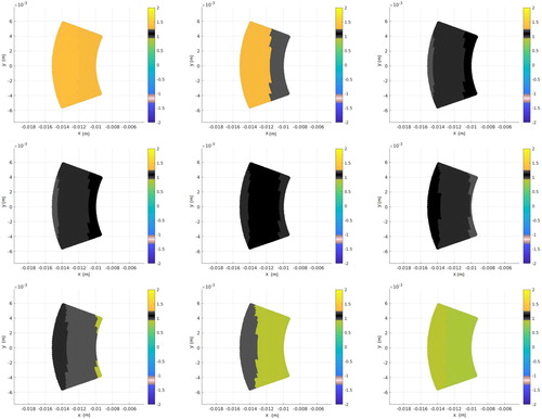
Figure 29. (a) Time-averaged relative error in region $D_1$. (b) Time-averaged absolute error in region $D_2$ over one period.

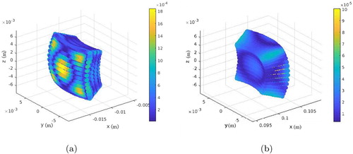
Figure 29 shows the averaged relative error on the primary control (a) and the averaged absolute error on the secondary control (b) over the entire time period. Notice that the time-averaged relative error in region $D_1$ is of magnitude ${10}^{-3}$ while the absolute error on region $D_2$ stays of order ${10}^{-4}$ showing the accuracy of our scheme over a range of frequencies.

5. Conclusions and future work

In this paper, we presented an improved numerical strategy for the control scheme described in [29] and employed it to perform several sensitivity studies for the scheme.

We have shown that for problem (2(2) $\begin{array}{rl}& \mathrm{\Delta }u+k^{2}u=0\text{ in }{\mathbb{R}}^3\setminus {\overline{D}}_a,\\ & \mathrm{\nabla }u\cdot \mathbf{n}=v_n,(\text{or }u=p_b)\text{ on }\mathrm{\partial }{D}_a,\\ & \left(\hat{\mathbf{x}},\mathrm{\nabla }u\left(\mathbf{x}\right)\right)-\mathrm{i}ku\left(\mathbf{x}\right)=o\left(\frac{1}{|\mathbf{x}|}\right),\text{ as }|\mathbf{x}|\to \mathrm{\infty }\text{ uniformly for all}\hat{\mathbf{x}},\end{array}$(2) ) and (3(3) $u\approx u_1\mathrm{in}{D}_1\mathrm{and}u\approx u_2=0\mathrm{in}{D}_2,$(3) ), in the configuration (1(1) $\begin{array}{rl}& \left(i\right)D_1\text{ bounded},D_2\text{ bounded},\\ & \left(ii\right)D_1\text{ bounded},D_2={\mathbb{R}}^3\setminus B_R\left(\mathbf{0}\right),\end{array}$(1) -ii), it is possible to characterize sources with weak far field and controllable fields in a compact near field region $D_1$. More explicitly, we should that surface sources could be characterized so that their radiated field approximate an incoming plane wave in a region of their near fields while maintaining a very small field beyond a finite radius. The sensitivity studies performed showed that the control scheme produces accurate results with respect to variations in the outward shift, outer radius and in both the outer and inner radii of the near control. Also, our numerics seem to suggest that it may be in principle possible to characterize surface sources with weak far fields so that they approximate prescribed Helmholtz potentials in larger subregions of their near field.

The control algorithm for problem (2(2) $\begin{array}{rl}& \mathrm{\Delta }u+k^{2}u=0\text{ in }{\mathbb{R}}^3\setminus {\overline{D}}_a,\\ & \mathrm{\nabla }u\cdot \mathbf{n}=v_n,(\text{or }u=p_b)\text{ on }\mathrm{\partial }{D}_a,\\ & \left(\hat{\mathbf{x}},\mathrm{\nabla }u\left(\mathbf{x}\right)\right)-\mathrm{i}ku\left(\mathbf{x}\right)=o\left(\frac{1}{|\mathbf{x}|}\right),\text{ as }|\mathbf{x}|\to \mathrm{\infty }\text{ uniformly for all}\hat{\mathbf{x}},\end{array}$(2) ) and (3(3) $u\approx u_1\mathrm{in}{D}_1\mathrm{and}u\approx u_2=0\mathrm{in}{D}_2,$(3) ) was also discussed in the configuration (1(1) $\begin{array}{rl}& \left(i\right)D_1\text{ bounded},D_2\text{ bounded},\\ & \left(ii\right)D_1\text{ bounded},D_2={\mathbb{R}}^3\setminus B_R\left(\mathbf{0}\right),\end{array}$(1) -ii). We considered first the situation when an outgoing plane wave was approximated in the near field region while maintaining a null in a prescribed region further away. The sensitivity analysis studied the scheme with respect to variations in the relative position of the control regions and showed very good accuracy results. For the same configuration, we also studied the case when a null was to be created in a near-field region while approximating an outgoing plane wave in a prescribed region further away and showed a food performance of our scheme. These results together with the superposition principle suggest that, in principle, our scheme could characterize surface sources so that their radiated fields will approximate distinct prescribed Helmholtz potentials in given mutually disjoint exterior regions of space.

In an effort to test our results in the time domain we considered again problem (2(2) $\begin{array}{rl}& \mathrm{\Delta }u+k^{2}u=0\text{ in }{\mathbb{R}}^3\setminus {\overline{D}}_a,\\ & \mathrm{\nabla }u\cdot \mathbf{n}=v_n,(\text{or }u=p_b)\text{ on }\mathrm{\partial }{D}_a,\\ & \left(\hat{\mathbf{x}},\mathrm{\nabla }u\left(\mathbf{x}\right)\right)-\mathrm{i}ku\left(\mathbf{x}\right)=o\left(\frac{1}{|\mathbf{x}|}\right),\text{ as }|\mathbf{x}|\to \mathrm{\infty }\text{ uniformly for all}\hat{\mathbf{x}},\end{array}$(2) ) and (3(3) $u\approx u_1\mathrm{in}{D}_1\mathrm{and}u\approx u_2=0\mathrm{in}{D}_2,$(3) ) in the configuration (1(1) $\begin{array}{rl}& \left(i\right)D_1\text{ bounded},D_2\text{ bounded},\\ & \left(ii\right)D_1\text{ bounded},D_2={\mathbb{R}}^3\setminus B_R\left(\mathbf{0}\right),\end{array}$(1) -ii) and employed the superposition principle to obtain a Fourier synthesis matching an outgoing plane wave in the primary near field control region in front of the source while keeping a low signature on a region further away behind the source. Our positive result is an indication that it may be possible to characterize such surface controls for time domain signals.

We believe that the study of the case when the source is an array, i.e. modelled as a union of compact mutually disjoint subdomains, is very important and our preliminary results in this regard are encouraging. We plan to present a detailed analysis of this case in a forthcoming paper.

An important feature of our work is mentioned in Remark 1 and Remark 2. Indeed, a first observation in this regard is that, as shown in Figure 2, Figure 19 and Figure 27, one could employ suitable optimization strategies for the description of the most feasible physical source boundary and this will be part of our related next research efforts. Another important point is that, as mentioned in the introduction, although our research characterizes continuous surface sources for their instantiation one could use monopole and dipole approximating arrays in the spirit of [31].

In the same spirit, a second important observation is that our analysis is not bounded to spherical fictitious regions $D_{a^{\prime }}$ as is presented in this paper. In fact one could in principle chose to start with an arbitrary smooth region $D_{a^{\prime }}$ by adapting the numerical analysis used to evaluate the propagator $\mathcal{D}$ and set up the optimization procedure. This will also be considered as part of our future investigations.

Last but not least, we mention that the sensitivity analysis performed in this paper together with the theory developed previously by our group in [28,29] are the foundation of our current efforts to extend the applicability of our scheme to the case of exterior surface control of vector fields which are solutions of the Maxwell equations. This part of our research is the current focus of our group and will be reported very soon.

Disclosure statement

No potential conflict of interest was reported by the authors.

Additional information

Funding

This work was initially supported by the Office of Naval Research under the award N00014-15-1-2462 and then supported by the Army Research Office under the award W911NF- 17-1-0478.

References

- Fuller C, von Flotow A. Active control of sound and vibration. IEEE Control Syst Mag. 1995;15(6):9–19. doi: 10.1109/37.476383
- Peake N, Crighton DG. Active control of sound. Annu Rev Fluid Mech. 2000;32:137–164. doi: 10.1146/annurev.fluid.32.1.137
- Elliott S. Signal processing for active control. 1st ed. London: Academic Press; 2000. (Signal Processing and its Applications).
- Nelson PA, Elliott SJ. Active control of sound. London: Academic Press; 1992.
- Olson HF, May EG. Electronic sound absorber. J Acad Soc Am. 1953;25:1130–1136. doi: 10.1121/1.1907249
- Cheer J, Elliott SJ. Multichannel control systems for the attenuation of interior road noise in vehicles. Mech Syst Signal Process. 2015;60–61:753–769. doi: 10.1016/j.ymssp.2015.01.008
- Kim Y, Choi J. Sound field reproduction. Hoboken: Wiley-Blackwell; 2013. Chapter 6; p. 283–370.
- Rabenstein R, Spors S. Sound field reproduction. In: Benesty J, Sondhi MM, Huang YA, editors. Springer handbook of speech processing. New York: Springer-Verlag; 2008. p. 1095–1114.
- Ahrens J, Spors S. Sound field reproduction using planar and linear arrays of loudspeakers. IEEE Trans Audio Speech Lang Process. 2010;18(8):2038–2050. doi: 10.1109/TASL.2010.2041106
- Ahrens J. Analytic methods of sound field synthesis. New York: Springer; 2012. (T-Labs Series in Telecommunications Services).
- Miller DAB. On perfect cloaking. Opt Express. 2006;14:12457–12466. doi: 10.1364/OE.14.012457
- Bobrovnitskii YI. A new impedance-based approach to analysis and control of sound scattering. J Sound Vib. 2006;297:743–760. doi: 10.1016/j.jsv.2006.04.030
- Bobrovnitskii YI. Impedance acoustic cloaking. New J Phys. 2010;12:043049. doi: 10.1088/1367-2630/12/4/043049
- Friot E, Guillermin R, Winninger M. Active control of scattered acoustic radiation: a real-time implementation for a three-dimensional object. Acta Acust United Acust. 2006;92:278–288.
- Noris AN. Acoustic cloaking. Acoustics Today. 2015;11(1):38–46.
- Vasquez FG, Milton GW, Onofrei D. Broadband exterior cloaking. Opt Exp. 2009;17(17):14800–14805. doi: 10.1364/OE.17.014800
- Vasquez FG, Milton GW, Onofrei D. Active exterior cloaking for the 2D Laplace and Helmholtz equations. Phys Rev Lett. 2009;103:073901. doi: 10.1103/PhysRevLett.103.073901
- Cheer J. Active control of scattered acoustic fields: cancellation, reproduction and cloaking. J Acoust Soc Am. 2016;140(3):1502–1512. doi: 10.1121/1.4962284
- Guevara Vasquez F, Milton GW, Onofrei D. Exterior cloaking with active sources in two dimensional acoustics. Wave Motion. 2011;48:515–524. doi: 10.1016/j.wavemoti.2011.03.005
- Lončarić J, Ryaben'kii VS, Tsynkov SV. Active shielding and control of noise. SIAM J Appl Math. 2001;62(2):563–596. doi: 10.1137/S0036139900367589
- Lončarić J, Tsynkov SV. Quadratic optimization in the problems of active control of sound. Appl Numer Math. 2005;52:381–400. doi: 10.1016/j.apnum.2004.08.041
- Olivieri F, Fazi F, Fontana S, et al. Generation of private sound with a circular loudspeaker array and the weighted pressure matching method. IEEE/ACM Trans Audio, Speech, Lang Process. 2017;5:1–21.
- Coleman P, Jackson PJB, Olik M, et al. Acoustic contrast, planarity and robustness of sound zone methods using a circular loudspeaker array. J Acoust Soc Am. 2014;135(4):1929–1940. doi: 10.1121/1.4866442
- Cai Y, Wu M, Yang J. Sound reproduction in personal audio systems using the least-squares approach with acoustic contrast control constraint. J Acoust Soc Am. 2014;135(2):734–741. doi: 10.1121/1.4861341
- Zhang W, Abhayapala TD, Betlehem T, et al. Analysis and control of multi-zone sound field reproduction using modal-domain approach. J Acoust Soc Am. 2016;140(3):2134–2144. doi: 10.1121/1.4963084
- Elliot SJ, Cheer J, Choi JW, et al. Robustness and regularization of personal audio systems. IEEE Trans Audio, Speech, Lang Process. 2012;20(7):2123–2133. doi: 10.1109/TASL.2012.2197613
- Poletti MA, Fazi FM. An approach to generating two zones of silence with application to personal sound systems. J Acoust Soc Am. 2015;137:598–605. doi: 10.1121/1.4906582
- Onofrei D. Active manipulation of fields modeled by the Helmholtz equation. J Integral Equ Appl. 2014;26(4):553–579. doi: 10.1216/JIE-2014-26-4-553
- Onofrei D, Platt E. On the synthesis of acoustic sources with controllable near fields. Wave Motion. 2018;77:12–27. doi: 10.1016/j.wavemoti.2017.10.004
- Onofrei D. On the active manipulation of fields and applications. I – the quasistatic regime. Inverse Probl. 2012;28(10):105009. doi: 10.1088/0266-5611/28/10/105009
- Doicu A, Eremin Y, Wriedt T. Acoustic and electromagnetic scattering analysis using discrete sources. London: Academic Press; 2000.
- Hubenthal M, Onofrei D. Sensitivity analysis for active control of the Helmholtz equation. Appl Numer Math. 2016;106:1–23. doi: 10.1016/j.apnum.2016.03.003
- Colton D, Kress R. Inverse acoustic and electromagnetic scattering theory. 3rd ed. New York: Springer-Verlag; 2013.
- Abramowitz M, Stegun IA. Handbook of mathematical functions with formulas, graphs and mathematical tables. 10th ed. Maryland: National Bureau of Standards; 1972. (Applied Mathematics Series 55).
- Watson GN. A treatise on the theory of Bessel functions. Cambridge: Cambridge University Press; 1906.
- https://drive.google.com/open?id=1m5nnofuIc56_aaU76HHjqkH4aRLRIsRi; 2018.