Reconstruction of the heat transfer coefficient at the interface of a bi-material

ABSTRACT

The knowledge of heat transfer behaviour of composite thermal systems requires the characterization of the heat transfer coefficient at the contact interfaces between the constituent materials. The present work is devoted to investigating an inverse problem with generalized interface condition containing an unknown space- and time-varying interface coefficient from non-invasive temperature measurements on an accessible boundary. The uniqueness of the solution holds, but the problem does not depend continuously on the input measured temperature data. A new preconditioned conjugate gradient method (CGM) is utilized to address the ill-posedness of the inverse problem. In comparison with the standard CGM with no preconditioning, this method has the merit that the gradient of the objective functional does not vanish at the final time, which restores accuracy and stability when the input data is contaminated with noise and when the initial guess is not close to the true solution. Several numerical examples corresponding to linear thermal contact and nonlinear Stefan-Boltzmann radiation condition are tested for determining thermal contact conductance and Stefan-Boltzmann coefficient, respectively. The numerical results in both one- and two-dimensions illustrate that the reconstructions are robust and stable.

KEYWORDS:

• Thermal contact conductance
• Stefan-Boltzmann coefficient
• preconditioning
• conjugate gradient method
• nonlinear inverse problem

SUBJECT CLASSIFICATION CODE:

• 65L09

1. Introduction

For many multi-layer composite materials and multi-component structures, the thermal behaviour is difficult to predict, due to the fact that the temperature at the interfaces is discontinuous. A crucial problem is the accurate predicition of the heat transfer coefficients (HTCs) at the solid-solid thermal contacting interfaces where the prescribed conditions can be linear [1] or nonlinear [2]. In this context, the knowledge of the thermal contact conductance (TCC) for a linear contact and the Stefan-Boltzmann coefficient (SBC) [3] for a nonlinear contact are essential. TCC is generally used to characterize the thermal resistance at the contacting region of two materials, owing to the effect of surface roughness. In addition, for some high-temperature applications [3–5], if there exists a tiny air layer between the mated surfaces, the Stefan-Boltzmann radiation condition should be applied. The parameter characterizing the effect of thermal radiation on the temperature drop is the SBC. Accurate estimates of TCC and SBC are of crucial importance for quality control and monitoring, and thus find applications in various fields, e.g. metal casting [1,6], heat exchangers [7], quenching of steel [8], plasma-facing components [9], measurement of blood perfusion [10] and defect detection [3].

For the determination of TCC, both analytical and experimental approaches have been throughly investigated. Some explicit expressions for TCC were proposed through direct analysis of deformation of asperities [11,12] and thermo-mechanical simulation [13]. However, the deviations between the analytical predictions and experimental measurements were observed, e.g. in [14,15]. Experimentally, the most straightforward way for the measurement of TCC is to use a series of thermocouples to measure the temperature profile along the center line, and then extrapolate it to the interface to obtain the temperature drop across the interface [13,15,16]. This type of method has some drawbacks of being sensitive to noise and time-consuming. Accordingly, many works reported are devoted to seek to retrieve a solution to an inverse heat conduction problem (IHCP) from few temperature measurements based on steady state [17,18] or transient heat transfer [1,14,19–21]. In the context of IHCPs, different techniques have been applied to address the ill-posedness of the inverse problem, e.g. the conjugate gradient method (CGM) [1,7,10,21], the Gauss-Newton algorithm [19], the function specification method [8,14] and the Tikhonov regularization [17]. More recently, Padilha et al. [22] developed an analytical method based on the reciprocity function [18,20] to solve the IHCP for the estimation of spatially-varying TCC, but no regularization method was considered.

When the boundary condition at the interface is nonlinear, the literature on the nonlinear IHCP for the reconstruction of SBC is rather scarce [3,5,23]. Hu et al. [5] reconstructed an inaccessible boundary of a three-layer composite material from Cauchy data on an accessible boundary and Stefan-Boltzmann radiation conditions at the interfaces. Wei [23] also investigated the boundary identification nonlinear problem with Stefan-Boltzmann interface condition, and showed rigorously the uniqueness of a moving boundary for this inverse problem. Murio [24] studied the numerical identification of an interface source function in a generalized nonlinear boundary condition by implementation of a stable space-marching finite difference method (FDM) in conjuction with mollification. In the aforementioned works, the SBC is a constant, but this assumption is not always appropriate, as it can vary spatially along the interface and even temporally, due to damages or thin coatings on the surface [25]. For this reason, Cheng et al. [3] studied an inverse problem of determining the space-dependent SBC and the defect area from temperature measurement on an observation surface. The reconstruction method proposed by them only works when the defect is located within the observation surface. However, a more general case of determining the SBC varying in both space and time domains has not been studied yet, as far as we know.

Our work aims to solve the generalized inverse problem of reconstructing the space and time-dependent interfacial coefficient (TCC or SBC) at the interface of a two-layer bicomponent composite material, from temperature measurements on an accessible portion of the exterior boundary of the bodies placed in contact. This is mathematically formulated in Section 2, where the uniqueness and the discontinuous dependence on the data of the solution are also briefly discussed. Compared to the previous one-dimensional (1D) inverse problems investigated in [1,7], our setting is formulated in any dimension hence, enabling practical 2D and 3D problems to be considered. Moreover, our result concerning the uniqueness of solution, that is sketched in Section 2.1, specifies sufficient data that can be measured, e.g. in the 1D case a boundary temperature measurement with one thermocouple at one end of the finite slab is sufficient, whilst Huang et al. [1] considered an extra intrusive internal thermocouple that is not actually needed for the uniqueness of solution, although of course adding more non-redundant information improves stability. Another major novelty of our study is that apart from the reconstruction of the TCC, we consider the numerical reconstruction of the SBC governing nonlinear fourth-order radiative contact. Within the numerical innovation, an important contribution of this paper is the development in Section 3 of a preconditioned CGM in a Hilbert space setting with inner product for the noise removal in the reconstructed solutions and overcoming the vanishing of the gradient at final time, encountered in the conventional CGM [1,7,26]. Moreover, note that in all the works mentioned above, the coefficient identification problems concerned homogeneous materials only. Hence, in this paper, we will consider the thermal properties as space-dependent to meet the potential application in functionally graded materials [27]. In order to test the performance of the proposed method, the numerical results of some benchmark examples are presented in Section 4 for both 1D and 2D problems. Finally, conclusions are given in Section 5.

2. Mathematical formulation

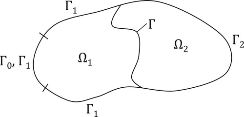
We consider a two-layer composite heat conductor $\mathrm{\Omega }={\mathrm{\Omega }}_1\cup {\mathrm{\Omega }}_2$, where ${\mathrm{\Omega }}_i$ is the ith subdomain with thermal conductivity $k_i$ and heat capacity per unit volume $C_i,i=1,2$. The thermal properties ($k_i$ and $C_i$) are assumed to be heterogeneous spacewise dependent known quantities. Let Γ be the interface between these two subdomains, and $\mathrm{\partial }{\mathrm{\Omega }}_i$ the boundary of the subdomain ${\mathrm{\Omega }}_i$. As shown in Figure 1, we have $\mathrm{\partial }{\mathrm{\Omega }}_1={\mathrm{\Gamma }}_1\cup \mathrm{\Gamma }$ and $\mathrm{\partial }{\mathrm{\Omega }}_2={\mathrm{\Gamma }}_2\cup \mathrm{\Gamma }$.

Figure 1. Schematic representation of the space bicomponent domain $\mathrm{\Omega }={\mathrm{\Omega }}_1\cup {\mathrm{\Omega }}_2$ in two-dimensions.

The heat conduction model is given by the heat equations, (1) $C_i\left(\mathbf{x}\right)\frac{\mathrm{\partial }{u}_i}{\mathrm{\partial }t}=\mathrm{\nabla }\cdot \left(k_i\right(\mathbf{x}\left)\mathrm{\nabla }{u}_i\right),(\mathbf{x},t)\in {\mathrm{\Omega }}_i\times (0,T),i=1,2$(1) with the Neumann heat flux boundary conditions, (2) $-k_i\left(\mathbf{x}\right)\frac{\mathrm{\partial }{u}_i}{\mathrm{\partial }{n}_i}=q_i(\mathbf{x},t),(\mathbf{x},t)\in {\mathrm{\Gamma }}_i\times (0,T),i=1,2$(2) the general interface condition, (3) $-k_1\left(\mathbf{x}\right)\frac{\mathrm{\partial }{u}_1}{\mathrm{\partial }{n}_1}=k_2\left(\mathbf{x}\right)\frac{\mathrm{\partial }{u}_2}{\mathrm{\partial }{n}_2}=\phi (\mathbf{x},t)\left[f\right(u_1)-f(u_2\left)\right],(\mathbf{x},t)\in \mathrm{\Gamma }\times (0,T),$(3) and initial conditions, (4) $u_i(\mathbf{x},0)=a_i\left(\mathbf{x}\right),\mathbf{x}\in {\mathrm{\Omega }}_i,i=1,2,$(4) where T>0 is the final time, $u_i$ is the temperature field in the domain ${\mathrm{\Omega }}_i$, ${\mathbf{n}}_i$ is the outward pointing unit normal vector to the boundary $\mathrm{\partial }{\mathrm{\Omega }}_i$, $q_i$ is the heat flux exerted on the boundary ${\mathrm{\Gamma }}_i$, $a_i\left(\mathbf{x}\right)$ is the initial temperature field in the domain ${\mathrm{\Omega }}_i$, for i=1,2, and, for simplicity, heat sources have been assumed absent. The materials ${\mathrm{\Omega }}_1$ and ${\mathrm{\Omega }}_2$ can be anisotropic in which case the scalars $k_1\left(\mathbf{x}\right)$ and $k_2\left(\mathbf{x}\right)$ become symmetric and positive definite tensors. Also, the Neumann boundary condition (2(2) $-k_i\left(\mathbf{x}\right)\frac{\mathrm{\partial }{u}_i}{\mathrm{\partial }{n}_i}=q_i(\mathbf{x},t),(\mathbf{x},t)\in {\mathrm{\Gamma }}_i\times (0,T),i=1,2$(2) ) can be replaced by more general Robin boundary conditions allowing for convection through the boundaries ${\mathrm{\Gamma }}_1$ and ${\mathrm{\Gamma }}_2$. Equation (3(3) $-k_1\left(\mathbf{x}\right)\frac{\mathrm{\partial }{u}_1}{\mathrm{\partial }{n}_1}=k_2\left(\mathbf{x}\right)\frac{\mathrm{\partial }{u}_2}{\mathrm{\partial }{n}_2}=\phi (\mathbf{x},t)\left[f\right(u_1)-f(u_2\left)\right],(\mathbf{x},t)\in \mathrm{\Gamma }\times (0,T),$(3) ) characterises a general condition at the interface Γ between the two heat conductors. If $f\left(u\right)=u$, the coefficient $\phi (\mathbf{x},t)$ represents the TCC. If $f\left(u\right)=u^4$, then Eq. (3(3) $-k_1\left(\mathbf{x}\right)\frac{\mathrm{\partial }{u}_1}{\mathrm{\partial }{n}_1}=k_2\left(\mathbf{x}\right)\frac{\mathrm{\partial }{u}_2}{\mathrm{\partial }{n}_2}=\phi (\mathbf{x},t)\left[f\right(u_1)-f(u_2\left)\right],(\mathbf{x},t)\in \mathrm{\Gamma }\times (0,T),$(3) ) is referred to as the Stefan-Boltzmann interface condition, and $\phi (\mathbf{x},t)$ is the SBC [3]. Both of these two conditions can cause a temperature discontinuity across the interface Γ.

The direct problem consists in the determination of the temperature fields $u_1$ and $u_2$ in the domains ${\mathrm{\Omega }}_1$ and ${\mathrm{\Omega }}_2$, from the knowledge of the geometry, thermal properties, boundary conditions, initial conditions and the interface coefficient. On the contrary, for the inverse problem, the space- and time-dependent coefficient $\phi (\mathbf{x},t)$ at the interface Γ and the temperature fields $u_1(\mathbf{x},t)$ and $u_2(\mathbf{x},t)$ are unknown and desired to be determined. Thus, we concentrate on determining $\phi (\mathbf{x},t)$, $u_1(\mathbf{x},t)$ and $u_2(\mathbf{x},t)$, given ${\mathrm{\Omega }}_i$, $k_i$, $C_i$, $q_i$, $a_i$, i=1,2, and the boundary temperature measurement on an accessible portion ${\mathrm{\Gamma }}_0\subset {\mathrm{\Gamma }}_1$, (5) $u_1({\mathbf{x}}_i,t)=Y({\mathbf{x}}_i,t),({\mathbf{x}}_i,t)\in {\mathrm{\Gamma }}_0\times (0,T),i=\overline{1,N_m},$(5) where $\mathbf{x}={\mathbf{x}}_i$ for $i=\overline{1,N_m}$ are the coordinates of $N_m$ measurement points on ${\mathrm{\Gamma }}_0$. The boundary ${\mathrm{\Gamma }}_0$ is assumed to be of positive measure and the temperature (5(5) $u_1({\mathbf{x}}_i,t)=Y({\mathbf{x}}_i,t),({\mathbf{x}}_i,t)\in {\mathrm{\Gamma }}_0\times (0,T),i=\overline{1,N_m},$(5) ) on it is measured experimentally (e.g. with a thermal camera), and taken as an overspecification condition to compensate for the missing information $\phi (\mathbf{x},t)$.

2.1. Ill-posedness of the inverse problem (1)–(5)

The uniqueness of solution of the inverse problem (1(1) $C_i\left(\mathbf{x}\right)\frac{\mathrm{\partial }{u}_i}{\mathrm{\partial }t}=\mathrm{\nabla }\cdot \left(k_i\right(\mathbf{x}\left)\mathrm{\nabla }{u}_i\right),(\mathbf{x},t)\in {\mathrm{\Omega }}_i\times (0,T),i=1,2$(1) )–(5(5) $u_1({\mathbf{x}}_i,t)=Y({\mathbf{x}}_i,t),({\mathbf{x}}_i,t)\in {\mathrm{\Gamma }}_0\times (0,T),i=\overline{1,N_m},$(5) ) holds, as sketched by the following argument. First, the uniqueness of solution of the inverse Cauchy problem for $u_1$ in ${\mathrm{\Omega }}_1\times (0,T)$ given by Eqs. (1(1) $C_i\left(\mathbf{x}\right)\frac{\mathrm{\partial }{u}_i}{\mathrm{\partial }t}=\mathrm{\nabla }\cdot \left(k_i\right(\mathbf{x}\left)\mathrm{\nabla }{u}_i\right),(\mathbf{x},t)\in {\mathrm{\Omega }}_i\times (0,T),i=1,2$(1) ), (2(2) $-k_i\left(\mathbf{x}\right)\frac{\mathrm{\partial }{u}_i}{\mathrm{\partial }{n}_i}=q_i(\mathbf{x},t),(\mathbf{x},t)\in {\mathrm{\Gamma }}_i\times (0,T),i=1,2$(2) ) and (4(4) $u_i(\mathbf{x},0)=a_i\left(\mathbf{x}\right),\mathbf{x}\in {\mathrm{\Omega }}_i,i=1,2,$(4) ) for i=1, and Eq. (5(5) $u_1({\mathbf{x}}_i,t)=Y({\mathbf{x}}_i,t),({\mathbf{x}}_i,t)\in {\mathrm{\Gamma }}_0\times (0,T),i=\overline{1,N_m},$(5) ) follows from the Holmgren theorem [5]. In fact, the initial condition (4(4) $u_i(\mathbf{x},0)=a_i\left(\mathbf{x}\right),\mathbf{x}\in {\mathrm{\Omega }}_i,i=1,2,$(4) ) with i=1 is not needed for this uniqueness analytic continuation argument. As a byproduct of this, it follows that $u_1{|}_{\mathrm{\Gamma }\times (0,T)}$ and $k_1\left(\mathrm{\partial }{u}_1/\mathrm{\partial }{n}_1\right){|}_{\mathrm{\Gamma }\times (0,T)}$ are uniquely determined. Then, the first identity in (3(3) $-k_1\left(\mathbf{x}\right)\frac{\mathrm{\partial }{u}_1}{\mathrm{\partial }{n}_1}=k_2\left(\mathbf{x}\right)\frac{\mathrm{\partial }{u}_2}{\mathrm{\partial }{n}_2}=\phi (\mathbf{x},t)\left[f\right(u_1)-f(u_2\left)\right],(\mathbf{x},t)\in \mathrm{\Gamma }\times (0,T),$(3) ) yields that $k_2\left(\mathrm{\partial }{u}_2/\mathrm{\partial }{n}_2\right){|}_{\mathrm{\Gamma }\times (0,T)}$ is also known and this, together with (2(2) $-k_i\left(\mathbf{x}\right)\frac{\mathrm{\partial }{u}_i}{\mathrm{\partial }{n}_i}=q_i(\mathbf{x},t),(\mathbf{x},t)\in {\mathrm{\Gamma }}_i\times (0,T),i=1,2$(2) ) and (4(4) $u_i(\mathbf{x},0)=a_i\left(\mathbf{x}\right),\mathbf{x}\in {\mathrm{\Omega }}_i,i=1,2,$(4) ) for i=2, form a direct well-posed Neumann problem for the heat equation for $u_2$ in ${\mathrm{\Omega }}_2\times (0,T)$. In particular, it yields that $u_2{|}_{\mathrm{\Gamma }\times (0,T)}$ is uniquely determined and finally, the interface coefficient is uniquely determined from (3(3) $-k_1\left(\mathbf{x}\right)\frac{\mathrm{\partial }{u}_1}{\mathrm{\partial }{n}_1}=k_2\left(\mathbf{x}\right)\frac{\mathrm{\partial }{u}_2}{\mathrm{\partial }{n}_2}=\phi (\mathbf{x},t)\left[f\right(u_1)-f(u_2\left)\right],(\mathbf{x},t)\in \mathrm{\Gamma }\times (0,T),$(3) ) as (6) $\phi =\frac{-k_1\frac{\mathrm{\partial }{u}_1}{\mathrm{\partial }{n}_1}}{f\left(u_1\right)-f\left(u_2\right)}\mathrm{on}\mathrm{\Gamma }\times (0,T),$(6) provided that the denominator is non-zero. Even if the uniqueness holds, the inverse problem (1(1) $C_i\left(\mathbf{x}\right)\frac{\mathrm{\partial }{u}_i}{\mathrm{\partial }t}=\mathrm{\nabla }\cdot \left(k_i\right(\mathbf{x}\left)\mathrm{\nabla }{u}_i\right),(\mathbf{x},t)\in {\mathrm{\Omega }}_i\times (0,T),i=1,2$(1) )–(5(5) $u_1({\mathbf{x}}_i,t)=Y({\mathbf{x}}_i,t),({\mathbf{x}}_i,t)\in {\mathrm{\Gamma }}_0\times (0,T),i=\overline{1,N_m},$(5) ) is still ill-posed since the interface coefficient φ does not depend continuously on the input measured data (5(5) $u_1({\mathbf{x}}_i,t)=Y({\mathbf{x}}_i,t),({\mathbf{x}}_i,t)\in {\mathrm{\Gamma }}_0\times (0,T),i=\overline{1,N_m},$(5) ). This can easily be seen from the following example of instability.

We consider a square domain Ω and take ${\mathrm{\Omega }}_1=(0,x_c)\times (0,L)$, ${\mathrm{\Omega }}_2=(x_c,L)\times (0,L)$, ${\mathrm{\Gamma }}_0=\left\{0\right\}\times (0,L)$, ${\mathrm{\Gamma }}_1=\left\{0\right\}\times (0,L)\cup (0,x_c)\times \{0,L\}$, ${\mathrm{\Gamma }}_2=\left\{L\right\}\times (0,L)\cup (x_c,L)\times \{0,L\}$, $\mathrm{\Gamma }=\left\{x_c\right\}\times (0,L)$, where $L=1/4$ and $x_c$ is a fixed value in $(0,L)$. The thermal properties of the materials are taken constant $k_1=k_2=c_1=c_2=1$. We take the function f in (3(3) $-k_1\left(\mathbf{x}\right)\frac{\mathrm{\partial }{u}_1}{\mathrm{\partial }{n}_1}=k_2\left(\mathbf{x}\right)\frac{\mathrm{\partial }{u}_2}{\mathrm{\partial }{n}_2}=\phi (\mathbf{x},t)\left[f\right(u_1)-f(u_2\left)\right],(\mathbf{x},t)\in \mathrm{\Gamma }\times (0,T),$(3) ) to be $f\left(u\right)=u^4$. With the initial temperatures $a_1(x,y)=p_1\cos \left(\alpha x\right)\cos \left(\pi y\right)$, $a_2(x,y)=p_2\cos \left(\alpha \right(x-L\left)\right)\cos \left(\pi y\right)$, the overspecified data $u_1(0,y,t)=Y(y,t)=p_1\cos \left(\pi y\right){\mathrm{e}}^{-mt}$, and the heat fluxes (7) $\begin{array}{rl}{q}_1(x,y,t)& =\left\{\begin{array}{ll}0,& \mathrm{on}x=0\mathrm{or}y=0,\\ \frac{\pi p_1}{\sqrt{2}}\cos \left(\alpha x\right){\mathrm{e}}^{-mt},& \mathrm{on}y=L,\end{array}\right.(x,y,t)\in {\mathrm{\Gamma }}_1\times (0,T),\end{array}$(7) (8) $\begin{array}{rl}{q}_2(x,y,t)& =\left\{\begin{array}{ll}0,& \mathrm{on}x=L\mathrm{or}y=0,\\ \frac{\pi p_2}{\sqrt{2}}\cos \left(\alpha \right(x-L\left)\right){\mathrm{e}}^{-mt},& \mathrm{on}y=L,\end{array}\right.(x,y,t)\in {\mathrm{\Gamma }}_2\times (0,T),\end{array}$(8) where $p_1=1/[\alpha \sin (\alpha x_c\left)\right]$, $p_2=1/[\alpha \sin (\alpha (x_c-L)\left)\right]$, $\alpha =\sqrt{m-{\pi }^2}$, $m\in \mathbb{N}$, $m\ge 10$, the temperatures $u_1$ and $u_2$ and the coefficient φ satisfying (1(1) $C_i\left(\mathbf{x}\right)\frac{\mathrm{\partial }{u}_i}{\mathrm{\partial }t}=\mathrm{\nabla }\cdot \left(k_i\right(\mathbf{x}\left)\mathrm{\nabla }{u}_i\right),(\mathbf{x},t)\in {\mathrm{\Omega }}_i\times (0,T),i=1,2$(1) )-(5(5) $u_1({\mathbf{x}}_i,t)=Y({\mathbf{x}}_i,t),({\mathbf{x}}_i,t)\in {\mathrm{\Gamma }}_0\times (0,T),i=\overline{1,N_m},$(5) ) are uniquely determined as, (9) $\begin{array}{ll}{u}_1(x,y,t)=p_1\cos \left(\alpha x\right)\cos \left(\pi y\right){\mathrm{e}}^{-mt},& (x,y,t)\in {\mathrm{\Omega }}_1\times (0,T),\\ u_2(x,y,t)=p_2\cos \left(\alpha \right(x-L\left)\right)\cos \left(\pi y\right)e^{-mt},& (x,y,t)\in {\mathrm{\Omega }}_2\times (0,T),\\ \phi (y,t)=\frac{e^{3mt}}{{\cos }^3\left(\pi y\right)}[p_1^4{\cos }^4(\alpha x_c)-p_2^4{\cos }^4(\alpha (x_c-L)){]}^{-1},& (y,t)\in [0,L]\times (0,T).\end{array}$(9) It can be seen from (9(9) $\begin{array}{ll}{u}_1(x,y,t)=p_1\cos \left(\alpha x\right)\cos \left(\pi y\right){\mathrm{e}}^{-mt},& (x,y,t)\in {\mathrm{\Omega }}_1\times (0,T),\\ u_2(x,y,t)=p_2\cos \left(\alpha \right(x-L\left)\right)\cos \left(\pi y\right)e^{-mt},& (x,y,t)\in {\mathrm{\Omega }}_2\times (0,T),\\ \phi (y,t)=\frac{e^{3mt}}{{\cos }^3\left(\pi y\right)}[p_1^4{\cos }^4(\alpha x_c)-p_2^4{\cos }^4(\alpha (x_c-L)){]}^{-1},& (y,t)\in [0,L]\times (0,T).\end{array}$(9) ) that, as $m\to \mathrm{\infty }$, the temperatures $u_1$ and $u_2$ tend to zero, as well as the input data $Y(y,t)$, while the interface coefficient φ becomes unbounded.

In order to cope with the ill-posedness of the inverse problem, we follow the framework of least-squares variational minimization, to reformulate it into a optimization problem, and then implement a regularization procedure, which is described in section 3, for restoring stability of the solution. The objective functional is defined as the $L^2$-norm of the residual between the calculated and measured temperature: (10) $J\left[\phi \right]=\frac{1}{2}\sum _{i=1}^{N_m}{∥u_1({\mathbf{x}}_i,t;\phi )-Y({\mathbf{x}}_i,t)∥}_{L^2\left(\right(0,T\left)\right)}^2,$(10) where $u({\mathbf{x}}_i,t;\phi )$ is the solution of the direct problem with respect to a particular function φ at ${\mathbf{x}}_i\in {\mathrm{\Gamma }}_0$, and $Y({\mathbf{x}}_i,t)$ is the corresponding measured temperature. The nonlinear least-squares function (10(10) $J\left[\phi \right]=\frac{1}{2}\sum _{i=1}^{N_m}{∥u_1({\mathbf{x}}_i,t;\phi )-Y({\mathbf{x}}_i,t)∥}_{L^2\left(\right(0,T\left)\right)}^2,$(10) ) is minimized by the preconditioned CGM, described in Section 3, in which a new gradient defined in a Hilbert space is used to generate the preconditioner.

3. Conjugate gradient method

The inverse problem of finding the triplet functions $\{u_1,u_2,\phi \}$ satisfying (1(1) $C_i\left(\mathbf{x}\right)\frac{\mathrm{\partial }{u}_i}{\mathrm{\partial }t}=\mathrm{\nabla }\cdot \left(k_i\right(\mathbf{x}\left)\mathrm{\nabla }{u}_i\right),(\mathbf{x},t)\in {\mathrm{\Omega }}_i\times (0,T),i=1,2$(1) )–(5(5) $u_1({\mathbf{x}}_i,t)=Y({\mathbf{x}}_i,t),({\mathbf{x}}_i,t)\in {\mathrm{\Gamma }}_0\times (0,T),i=\overline{1,N_m},$(5) ) is nonlinear, and we introduce the conjugate gradient method (CGM) to solve this problem. The idea of the CGM for the desired interface coefficient φ is to minimize the objective functional (10(10) $J\left[\phi \right]=\frac{1}{2}\sum _{i=1}^{N_m}{∥u_1({\mathbf{x}}_i,t;\phi )-Y({\mathbf{x}}_i,t)∥}_{L^2\left(\right(0,T\left)\right)}^2,$(10) ) by using the following recurrence relationship: (11) ${\phi }^{n+1}(\mathbf{x},t)={\phi }^n(\mathbf{x},t)-{\beta }^n{d}^n(\mathbf{x},t),n=0,1,\dots ,$(11) where the superscript n is the iteration number and ${\phi }^0$ is an initial guess, ${\beta }^n$ is the search step size at nth iteration, and $d^n(\mathbf{x},t)$ is the direction of descent defined recurrently as, (12) $d^0(\mathbf{x},t)=J^{\mathrm{\prime }}\left[{\phi }^0\right],d^n(\mathbf{x},t)=J^{\mathrm{\prime }}\left[{\phi }^n\right]+{\gamma }^n{d}^{n-1}(\mathbf{x},t),n=1,2,\dots ,$(12) where $J^{\mathrm{\prime }}\left[{\phi }^n\right]$ stands for the gradient of the functional J with respect to φ, and ${\gamma }^n$ is the conjugate coefficient. Although there are many choices for ${\gamma }^n$, here we use the Polak-Ribiere method, due to its computational performance [28], (13) ${\gamma }^n=\frac{⟨J^{\mathrm{\prime }}\left[{\phi }^n\right],J^{\mathrm{\prime }}\left[{\phi }^n\right]-J^{\mathrm{\prime }}\left[{\phi }^{n-1}\right]{⟩}_{L^2(\mathrm{\Gamma }\times (0,T\left)\right)}}{\parallel J^{\mathrm{\prime }}\left[{\phi }^{n-1}\right]{\parallel }_{L^2(\mathrm{\Gamma }\times (0,T\left)\right)}^2},n=1,2,\dots ,$(13) where $⟨\cdot ,\cdot {⟩}_{L^2}$ denotes the $L^2$-inner product.

Further, the search step size ${\beta }^n$ is chosen as the one that minimizes the objective functional J at each iteration, (14) ${\beta }^n=\underset{\beta }{\arg \min }J[{\phi }^n-\beta d^n].$(14) By following a similar analysis to that of [29], ${\beta }^n$ is obtained as, (15) ${\beta }^n=\frac{\sum _{i=1}^{N_m}⟨u_1({\mathbf{x}}_i,t;{\phi }^n)-Y({\mathbf{x}}_i,t),\mathrm{\Delta }{u}_1^n({\mathbf{x}}_i,t){⟩}_{L^2(0,T)}}{\sum _{i=1}^{N_m}\parallel \mathrm{\Delta }{u}_1^n({\mathbf{x}}_i,t){\parallel }_{L^2(0,T)}^2},n=0,1,\dots ,$(15) where $\mathrm{\Delta }{u}_1^n({\mathbf{x}}_i,t)=\mathrm{\Delta }{u}_1({\mathbf{x}}_i,t;d^n)$, $i=\overline{1,N_m}$, is the solution to a sensitivity problem presented in Section 3.1 with $\mathrm{\Delta }{\phi }^n=d^n$. In order to obtain the gradient $J^{\mathrm{\prime }}\left[{\phi }^n\right]$, the solution to an adjoint problem is required, which will be introduced in Section 3.2.

3.1. The sensitivity problem

To obtain the search step size via Eq. (15(15) ${\beta }^n=\frac{\sum _{i=1}^{N_m}⟨u_1({\mathbf{x}}_i,t;{\phi }^n)-Y({\mathbf{x}}_i,t),\mathrm{\Delta }{u}_1^n({\mathbf{x}}_i,t){⟩}_{L^2(0,T)}}{\sum _{i=1}^{N_m}\parallel \mathrm{\Delta }{u}_1^n({\mathbf{x}}_i,t){\parallel }_{L^2(0,T)}^2},n=0,1,\dots ,$(15) ), a sensitivity problem is constructed. By adding a perturbation $\epsilon \mathrm{\Delta }\phi (\mathbf{x},t)$ to $\phi (\mathbf{x},t)$, the subsequent responses $u_1(\mathbf{x},t)$ and $u_2(\mathbf{x},t)$ are perturbed by $\epsilon \mathrm{\Delta }{u}_1(\mathbf{x},t)$ and $\epsilon \mathrm{\Delta }{u}_2(\mathbf{x},t)$, respectively, where ϵ is a small parameter. By replacing $u_1$, $u_2$ and φ in the direct problem (1(1) $C_i\left(\mathbf{x}\right)\frac{\mathrm{\partial }{u}_i}{\mathrm{\partial }t}=\mathrm{\nabla }\cdot \left(k_i\right(\mathbf{x}\left)\mathrm{\nabla }{u}_i\right),(\mathbf{x},t)\in {\mathrm{\Omega }}_i\times (0,T),i=1,2$(1) )–(4(4) $u_i(\mathbf{x},0)=a_i\left(\mathbf{x}\right),\mathbf{x}\in {\mathrm{\Omega }}_i,i=1,2,$(4) ) by $(u_1+\epsilon \mathrm{\Delta }{u}_1)$, $(u_2+\epsilon \mathrm{\Delta }{u}_2)$ and $(\phi +\epsilon \mathrm{\Delta }\phi )$, respectively, and comparing the resulting formulation with the original direct problem, one can obtain the following sensitivity problem: (16) $\begin{array}{ll}{C}_i\left(\mathbf{x}\right)\frac{\mathrm{\partial }\left(\mathrm{\Delta }{u}_i\right)}{\mathrm{\partial }t}=\mathrm{\nabla }\cdot \left(k_i\right(\mathbf{x}\left)\mathrm{\nabla }\right(\mathrm{\Delta }{u}_i\left)\right),& (\mathbf{x},t)\in {\mathrm{\Omega }}_i\times (0,T),\\ -k_i\left(\mathbf{x}\right)\frac{\mathrm{\partial }\left(\mathrm{\Delta }{u}_i\right)}{\mathrm{\partial }{n}_i}=0,& (\mathbf{x},t)\in {\mathrm{\Gamma }}_i\times (0,T),\\ \mathrm{\Delta }{u}_i(\mathbf{x},0)=0,& \mathbf{x}\in {\mathrm{\Omega }}_i,i=1,2\end{array}$(16) with the interface condition, (17) $\begin{array}{rl}-k_1\left(\mathbf{x}\right)\frac{\mathrm{\partial }\left(\mathrm{\Delta }{u}_1\right)}{\mathrm{\partial }{n}_1}& =k_2\left(\mathbf{x}\right)\frac{\mathrm{\partial }\left(\mathrm{\Delta }{u}_2\right)}{\mathrm{\partial }{n}_2}=\phi (\mathbf{x},t)\left[f^{\mathrm{\prime }}\right(u_1)\mathrm{\Delta }{u}_1-f^{\mathrm{\prime }}(u_2\left)\mathrm{\Delta }{u}_2\right]\\ & +\mathrm{\Delta }\phi (\mathbf{x},t)\left[f\right(u_1)-f(u_2\left)\right],(\mathbf{x},t)\in \mathrm{\Gamma }\times (0,T),\end{array}$(17) where we have neglected the second-order terms of order ${\epsilon }^2$ and made the first-order approximation $f(u+\epsilon \mathrm{\Delta }u)\approx f\left(u\right)+\epsilon f^{\mathrm{\prime }}\left(u\right)\mathrm{\Delta }u$.

3.2. The adjoint problem

Due to the constraint that the temperature $u_1(\mathbf{x},t;\phi )$ in the objective functional (10(10) $J\left[\phi \right]=\frac{1}{2}\sum _{i=1}^{N_m}{∥u_1({\mathbf{x}}_i,t;\phi )-Y({\mathbf{x}}_i,t)∥}_{L^2\left(\right(0,T\left)\right)}^2,$(10) ) is the solution of the direct problem, we introduce two Lagrange multipliers ${\lambda }_1(\mathbf{x},t)$ and ${\lambda }_2(\mathbf{x},t)$ to construct the constrained objective functional, (18) $\begin{array}{rl}J\left[\phi \right]& =\frac{1}{2}\sum _{i=1}^{N_m}{\int }_0^T{\left[u_1({\mathbf{x}}_i,t;\phi )-Y({\mathbf{x}}_i,t)\right]}^{2}dt+{\int }_{{\mathrm{\Omega }}_1}{\int }_0^T{\lambda }_1\left[C_1\frac{\mathrm{\partial }{u}_1}{\mathrm{\partial }t}-\mathrm{\nabla }\cdot \left(k_1\mathrm{\nabla }{u}_1\right)\right]\mathrm{d}t\mathrm{d}\mathbf{x}\\ & +{\int }_{{\mathrm{\Omega }}_2}{\int }_0^T{\lambda }_2\left[C_2\frac{\mathrm{\partial }{u}_2}{\mathrm{\partial }t}-\mathrm{\nabla }\cdot \left(k_2\mathrm{\nabla }{u}_2\right)\right]\mathrm{d}t\mathrm{d}\mathbf{x}.\end{array}$(18) The functional $J\left[\phi \right]$ has a variation $\mathrm{\Delta }J\left[\phi \right]$ corresponding to the perturbation of φ. Note that $\mathrm{\Delta }J\left[\phi \right]$ is the directional derivative of $J\left[\phi \right]$ in the direction of $\mathrm{\Delta }\phi$, [29], and thus can be derived from Eq. (18(18) $\begin{array}{rl}J\left[\phi \right]& =\frac{1}{2}\sum _{i=1}^{N_m}{\int }_0^T{\left[u_1({\mathbf{x}}_i,t;\phi )-Y({\mathbf{x}}_i,t)\right]}^{2}dt+{\int }_{{\mathrm{\Omega }}_1}{\int }_0^T{\lambda }_1\left[C_1\frac{\mathrm{\partial }{u}_1}{\mathrm{\partial }t}-\mathrm{\nabla }\cdot \left(k_1\mathrm{\nabla }{u}_1\right)\right]\mathrm{d}t\mathrm{d}\mathbf{x}\\ & +{\int }_{{\mathrm{\Omega }}_2}{\int }_0^T{\lambda }_2\left[C_2\frac{\mathrm{\partial }{u}_2}{\mathrm{\partial }t}-\mathrm{\nabla }\cdot \left(k_2\mathrm{\nabla }{u}_2\right)\right]\mathrm{d}t\mathrm{d}\mathbf{x}.\end{array}$(18) ) as follows: (19) $\begin{array}{rl}\mathrm{\Delta }J\left[\phi \right]& =\sum _{i=1}^{N_m}{\int }_{{\mathrm{\Omega }}_1}{\int }_0^T\mathrm{\Delta }{u}_1\left[u_1(\mathbf{x},t;\phi )-Y({\mathbf{x}}_i,t)\right]\delta (\mathbf{x}-{\mathbf{x}}_i)\mathrm{d}t\mathrm{d}\mathbf{x}\\ & +{\int }_{{\mathrm{\Omega }}_1}{\int }_0^T{\lambda }_1\left[C_1\frac{\mathrm{\partial }\left(\mathrm{\Delta }{u}_1\right)}{\mathrm{\partial }t}-\mathrm{\nabla }\cdot \left(k_1\mathrm{\nabla }\right(\mathrm{\Delta }{u}_1\left)\right)\right]\mathrm{d}t\mathrm{d}\mathbf{x}\\ & +{\int }_{{\mathrm{\Omega }}_2}{\int }_0^T{\lambda }_2\left[C_2\frac{\mathrm{\partial }\left(\mathrm{\Delta }{u}_2\right)}{\mathrm{\partial }t}-\mathrm{\nabla }\cdot \left(k_2\mathrm{\nabla }\right(\mathrm{\Delta }{u}_2\left)\right)\right]\mathrm{d}t\mathrm{d}\mathbf{x},\end{array}$(19) where $\delta (\cdot )$ is the Dirac delta function. One can further simplify the second and third integrals on the right-hand side of Eq. (19(19) $\begin{array}{rl}\mathrm{\Delta }J\left[\phi \right]& =\sum _{i=1}^{N_m}{\int }_{{\mathrm{\Omega }}_1}{\int }_0^T\mathrm{\Delta }{u}_1\left[u_1(\mathbf{x},t;\phi )-Y({\mathbf{x}}_i,t)\right]\delta (\mathbf{x}-{\mathbf{x}}_i)\mathrm{d}t\mathrm{d}\mathbf{x}\\ & +{\int }_{{\mathrm{\Omega }}_1}{\int }_0^T{\lambda }_1\left[C_1\frac{\mathrm{\partial }\left(\mathrm{\Delta }{u}_1\right)}{\mathrm{\partial }t}-\mathrm{\nabla }\cdot \left(k_1\mathrm{\nabla }\right(\mathrm{\Delta }{u}_1\left)\right)\right]\mathrm{d}t\mathrm{d}\mathbf{x}\\ & +{\int }_{{\mathrm{\Omega }}_2}{\int }_0^T{\lambda }_2\left[C_2\frac{\mathrm{\partial }\left(\mathrm{\Delta }{u}_2\right)}{\mathrm{\partial }t}-\mathrm{\nabla }\cdot \left(k_2\mathrm{\nabla }\right(\mathrm{\Delta }{u}_2\left)\right)\right]\mathrm{d}t\mathrm{d}\mathbf{x},\end{array}$(19) ), using integration by parts, into the following: (20) $\begin{array}{rl}{I}_i& ={\int }_{{\mathrm{\Omega }}_i}{\int }_0^T{\lambda }_i\left[C_i\frac{\mathrm{\partial }\left(\mathrm{\Delta }{u}_i\right)}{\mathrm{\partial }t}-\mathrm{\nabla }\cdot \left(k_i\mathrm{\nabla }\right(\mathrm{\Delta }{u}_i\left)\right)\right]\mathrm{d}t\mathrm{d}\mathbf{x}\\ & ={\left.{\int }_{{\mathrm{\Omega }}_i}{C}_i{\lambda }_i\mathrm{\Delta }{u}_i\right|}_0^T\mathrm{d}\mathbf{x}-{\int }_{{\mathrm{\Omega }}_i}{\int }_0^T{C}_i\mathrm{\Delta }{u}_i\frac{\mathrm{\partial }{\lambda }_i}{\mathrm{\partial }t}\mathrm{d}t\mathrm{d}\mathbf{x}-{\int }_{\mathrm{\partial }{\mathrm{\Omega }}_i}{\int }_0^T{k}_i{\lambda }_i\frac{\mathrm{\partial }\left(\mathrm{\Delta }{u}_i\right)}{\mathrm{\partial }{n}_i}\mathrm{d}t\mathrm{d}s\\ & +{\int }_{\mathrm{\partial }{\mathrm{\Omega }}_i}{\int }_0^T{k}_i\mathrm{\Delta }{u}_i\frac{\mathrm{\partial }{\lambda }_i}{\mathrm{\partial }{n}_i}\mathrm{d}t\mathrm{d}s-{\int }_{{\mathrm{\Omega }}_i}{\int }_0^T\mathrm{\Delta }{u}_i\mathrm{\nabla }\cdot \left(k_i\mathrm{\nabla }{\lambda }_i\right)\mathrm{d}t\mathrm{d}\mathbf{x},i=1,2.\end{array}$(20) Substituting Eqs. (20(20) $\begin{array}{rl}{I}_i& ={\int }_{{\mathrm{\Omega }}_i}{\int }_0^T{\lambda }_i\left[C_i\frac{\mathrm{\partial }\left(\mathrm{\Delta }{u}_i\right)}{\mathrm{\partial }t}-\mathrm{\nabla }\cdot \left(k_i\mathrm{\nabla }\right(\mathrm{\Delta }{u}_i\left)\right)\right]\mathrm{d}t\mathrm{d}\mathbf{x}\\ & ={\left.{\int }_{{\mathrm{\Omega }}_i}{C}_i{\lambda }_i\mathrm{\Delta }{u}_i\right|}_0^T\mathrm{d}\mathbf{x}-{\int }_{{\mathrm{\Omega }}_i}{\int }_0^T{C}_i\mathrm{\Delta }{u}_i\frac{\mathrm{\partial }{\lambda }_i}{\mathrm{\partial }t}\mathrm{d}t\mathrm{d}\mathbf{x}-{\int }_{\mathrm{\partial }{\mathrm{\Omega }}_i}{\int }_0^T{k}_i{\lambda }_i\frac{\mathrm{\partial }\left(\mathrm{\Delta }{u}_i\right)}{\mathrm{\partial }{n}_i}\mathrm{d}t\mathrm{d}s\\ & +{\int }_{\mathrm{\partial }{\mathrm{\Omega }}_i}{\int }_0^T{k}_i\mathrm{\Delta }{u}_i\frac{\mathrm{\partial }{\lambda }_i}{\mathrm{\partial }{n}_i}\mathrm{d}t\mathrm{d}s-{\int }_{{\mathrm{\Omega }}_i}{\int }_0^T\mathrm{\Delta }{u}_i\mathrm{\nabla }\cdot \left(k_i\mathrm{\nabla }{\lambda }_i\right)\mathrm{d}t\mathrm{d}\mathbf{x},i=1,2.\end{array}$(20) ), and the boundary conditions and initial conditions of the sensitivity problem (16(16) $\begin{array}{ll}{C}_i\left(\mathbf{x}\right)\frac{\mathrm{\partial }\left(\mathrm{\Delta }{u}_i\right)}{\mathrm{\partial }t}=\mathrm{\nabla }\cdot \left(k_i\right(\mathbf{x}\left)\mathrm{\nabla }\right(\mathrm{\Delta }{u}_i\left)\right),& (\mathbf{x},t)\in {\mathrm{\Omega }}_i\times (0,T),\\ -k_i\left(\mathbf{x}\right)\frac{\mathrm{\partial }\left(\mathrm{\Delta }{u}_i\right)}{\mathrm{\partial }{n}_i}=0,& (\mathbf{x},t)\in {\mathrm{\Gamma }}_i\times (0,T),\\ \mathrm{\Delta }{u}_i(\mathbf{x},0)=0,& \mathbf{x}\in {\mathrm{\Omega }}_i,i=1,2\end{array}$(16) ) into (19(19) $\begin{array}{rl}\mathrm{\Delta }J\left[\phi \right]& =\sum _{i=1}^{N_m}{\int }_{{\mathrm{\Omega }}_1}{\int }_0^T\mathrm{\Delta }{u}_1\left[u_1(\mathbf{x},t;\phi )-Y({\mathbf{x}}_i,t)\right]\delta (\mathbf{x}-{\mathbf{x}}_i)\mathrm{d}t\mathrm{d}\mathbf{x}\\ & +{\int }_{{\mathrm{\Omega }}_1}{\int }_0^T{\lambda }_1\left[C_1\frac{\mathrm{\partial }\left(\mathrm{\Delta }{u}_1\right)}{\mathrm{\partial }t}-\mathrm{\nabla }\cdot \left(k_1\mathrm{\nabla }\right(\mathrm{\Delta }{u}_1\left)\right)\right]\mathrm{d}t\mathrm{d}\mathbf{x}\\ & +{\int }_{{\mathrm{\Omega }}_2}{\int }_0^T{\lambda }_2\left[C_2\frac{\mathrm{\partial }\left(\mathrm{\Delta }{u}_2\right)}{\mathrm{\partial }t}-\mathrm{\nabla }\cdot \left(k_2\mathrm{\nabla }\right(\mathrm{\Delta }{u}_2\left)\right)\right]\mathrm{d}t\mathrm{d}\mathbf{x},\end{array}$(19) ), we obtain, (21) $\begin{array}{rl}\mathrm{\Delta }J\left[\phi \right]& =\sum _{i=1}^{N_m}{\int }_{{\mathrm{\Omega }}_1}{\int }_0^T\mathrm{\Delta }{u}_1\left[u_1(\mathbf{x},t;\phi )-Y({\mathbf{x}}_i,t)\right]\delta (\mathbf{x}-{\mathbf{x}}_i)\mathrm{d}t\mathrm{d}\mathbf{x}\\ & +\sum _{i=1}^2\left[{\int }_{{\mathrm{\Omega }}_i}{C}_i{\lambda }_i(\mathbf{x},T)\mathrm{\Delta }{u}_i\mathrm{d}\mathbf{x}-{\int }_{{\mathrm{\Omega }}_i}{\int }_0^T\mathrm{\Delta }{u}_i\left(C_i\frac{\mathrm{\partial }{\lambda }_i}{\mathrm{\partial }t}+\mathrm{\nabla }\cdot \left(k_i\mathrm{\nabla }{\lambda }_i\right)\right)\mathrm{d}t\mathrm{d}\mathbf{x}\right.\\ & \left.-{\int }_{\mathrm{\Gamma }}{\int }_0^T{k}_i{\lambda }_i\frac{\mathrm{\partial }\left(\mathrm{\Delta }{u}_i\right)}{\mathrm{\partial }{n}_i}\mathrm{d}t\mathrm{d}s+{\int }_{\mathrm{\partial }{\mathrm{\Omega }}_i}{\int }_0^T{k}_i\mathrm{\Delta }{u}_i\frac{\mathrm{\partial }{\lambda }_i}{\mathrm{\partial }{n}_i}\mathrm{d}t\mathrm{d}s\right].\end{array}$(21) Let the terms in Eq. (21(21) $\begin{array}{rl}\mathrm{\Delta }J\left[\phi \right]& =\sum _{i=1}^{N_m}{\int }_{{\mathrm{\Omega }}_1}{\int }_0^T\mathrm{\Delta }{u}_1\left[u_1(\mathbf{x},t;\phi )-Y({\mathbf{x}}_i,t)\right]\delta (\mathbf{x}-{\mathbf{x}}_i)\mathrm{d}t\mathrm{d}\mathbf{x}\\ & +\sum _{i=1}^2\left[{\int }_{{\mathrm{\Omega }}_i}{C}_i{\lambda }_i(\mathbf{x},T)\mathrm{\Delta }{u}_i\mathrm{d}\mathbf{x}-{\int }_{{\mathrm{\Omega }}_i}{\int }_0^T\mathrm{\Delta }{u}_i\left(C_i\frac{\mathrm{\partial }{\lambda }_i}{\mathrm{\partial }t}+\mathrm{\nabla }\cdot \left(k_i\mathrm{\nabla }{\lambda }_i\right)\right)\mathrm{d}t\mathrm{d}\mathbf{x}\right.\\ & \left.-{\int }_{\mathrm{\Gamma }}{\int }_0^T{k}_i{\lambda }_i\frac{\mathrm{\partial }\left(\mathrm{\Delta }{u}_i\right)}{\mathrm{\partial }{n}_i}\mathrm{d}t\mathrm{d}s+{\int }_{\mathrm{\partial }{\mathrm{\Omega }}_i}{\int }_0^T{k}_i\mathrm{\Delta }{u}_i\frac{\mathrm{\partial }{\lambda }_i}{\mathrm{\partial }{n}_i}\mathrm{d}t\mathrm{d}s\right].\end{array}$(21) ) containing $\mathrm{\Delta }{u}_1$ and $\mathrm{\Delta }{u}_2$ vanish and utilize the interface condition (17(17) $\begin{array}{rl}-k_1\left(\mathbf{x}\right)\frac{\mathrm{\partial }\left(\mathrm{\Delta }{u}_1\right)}{\mathrm{\partial }{n}_1}& =k_2\left(\mathbf{x}\right)\frac{\mathrm{\partial }\left(\mathrm{\Delta }{u}_2\right)}{\mathrm{\partial }{n}_2}=\phi (\mathbf{x},t)\left[f^{\mathrm{\prime }}\right(u_1)\mathrm{\Delta }{u}_1-f^{\mathrm{\prime }}(u_2\left)\mathrm{\Delta }{u}_2\right]\\ & +\mathrm{\Delta }\phi (\mathbf{x},t)\left[f\right(u_1)-f(u_2\left)\right],(\mathbf{x},t)\in \mathrm{\Gamma }\times (0,T),\end{array}$(17) ), to obtain the adjoint problems, (22) $\begin{array}{l}{C}_1\left(\mathbf{x}\right)\frac{\mathrm{\partial }{\lambda }_1}{\mathrm{\partial }t}+\mathrm{\nabla }\cdot \left(k_1\right(\mathbf{x}\left)\mathrm{\nabla }{\lambda }_1\right)\\ =\sum _{i=1}^{N_m}\left[u_1\right(\mathbf{x},t;\phi )-Y({\mathbf{x}}_i,t\left)\right]\delta (\mathbf{x}-{\mathbf{x}}_i),& (\mathbf{x},t)\in {\mathrm{\Omega }}_1\times (0,T),\\ \frac{\mathrm{\partial }{\lambda }_1}{\mathrm{\partial }{n}_1}=0,& (\mathbf{x},t)\in {\mathrm{\Gamma }}_1\times (0,T),\\ {\lambda }_1(\mathbf{x},T)=0,& \mathbf{x}\in {\mathrm{\Omega }}_1,\\ -k_1\left(\mathbf{x}\right)\frac{\mathrm{\partial }{\lambda }_1}{\mathrm{\partial }{n}_1}=\phi (\mathbf{x},t)f^{\mathrm{\prime }}\left(u_1\right)\left[{\lambda }_1\right(\mathbf{x},t)-{\lambda }_2(\mathbf{x},t\left)\right],& (\mathbf{x},t)\in \mathrm{\Gamma }\times (0,T),\end{array}$(22) and (23) $\begin{array}{ll}{C}_2\left(\mathbf{x}\right)\frac{\mathrm{\partial }{\lambda }_2}{\mathrm{\partial }t}+\mathrm{\nabla }\cdot \left(k_2\right(\mathbf{x}\left)\mathrm{\nabla }{\lambda }_2\right)=0,& (\mathbf{x},t)\in {\mathrm{\Omega }}_2\times (0,T),\\ \frac{\mathrm{\partial }{\lambda }_2}{\mathrm{\partial }{n}_2}=0,& (\mathbf{x},t)\in {\mathrm{\Gamma }}_2\times (0,T),\\ {\lambda }_2(\mathbf{x},T)=0,& \mathbf{x}\in {\mathrm{\Omega }}_2,\\ k_2\left(\mathbf{x}\right)\frac{\mathrm{\partial }{\lambda }_2}{\mathrm{\partial }{n}_2}=\phi (\mathbf{x},t)f^{\mathrm{\prime }}\left(u_2\right)\left[{\lambda }_1\right(\mathbf{x},t)-{\lambda }_2(\mathbf{x},t\left)\right],& (\mathbf{x},t)\in \mathrm{\Gamma }\times (0,T).\end{array}$(23) Consequently, Eq. (21(21) $\begin{array}{rl}\mathrm{\Delta }J\left[\phi \right]& =\sum _{i=1}^{N_m}{\int }_{{\mathrm{\Omega }}_1}{\int }_0^T\mathrm{\Delta }{u}_1\left[u_1(\mathbf{x},t;\phi )-Y({\mathbf{x}}_i,t)\right]\delta (\mathbf{x}-{\mathbf{x}}_i)\mathrm{d}t\mathrm{d}\mathbf{x}\\ & +\sum _{i=1}^2\left[{\int }_{{\mathrm{\Omega }}_i}{C}_i{\lambda }_i(\mathbf{x},T)\mathrm{\Delta }{u}_i\mathrm{d}\mathbf{x}-{\int }_{{\mathrm{\Omega }}_i}{\int }_0^T\mathrm{\Delta }{u}_i\left(C_i\frac{\mathrm{\partial }{\lambda }_i}{\mathrm{\partial }t}+\mathrm{\nabla }\cdot \left(k_i\mathrm{\nabla }{\lambda }_i\right)\right)\mathrm{d}t\mathrm{d}\mathbf{x}\right.\\ & \left.-{\int }_{\mathrm{\Gamma }}{\int }_0^T{k}_i{\lambda }_i\frac{\mathrm{\partial }\left(\mathrm{\Delta }{u}_i\right)}{\mathrm{\partial }{n}_i}\mathrm{d}t\mathrm{d}s+{\int }_{\mathrm{\partial }{\mathrm{\Omega }}_i}{\int }_0^T{k}_i\mathrm{\Delta }{u}_i\frac{\mathrm{\partial }{\lambda }_i}{\mathrm{\partial }{n}_i}\mathrm{d}t\mathrm{d}s\right].\end{array}$(21) ) is simplified as: (24) $\mathrm{\Delta }J\left[\phi \right]={\int }_{\mathrm{\Gamma }}{\int }_0^T\mathrm{\Delta }\phi \left[f\right(u_1(\mathbf{x},t))-f(u_2(\mathbf{x},t)\left)\right]\left[{\lambda }_1\right(\mathbf{x},t)-{\lambda }_2(\mathbf{x},t\left)\right]\mathrm{d}t\mathrm{d}s,$(24) and thus the $L^2$-gradient of the functional $J\left[\phi \right]$ is, (25) $J_L^{\mathrm{\prime }}\left[\phi \right]=\left[f\right(u_1(\mathbf{x},t))-f(u_2(\mathbf{x},t)\left)\right]\left[{\lambda }_1\right(\mathbf{x},t)-{\lambda }_2(\mathbf{x},t\left)\right],(\mathbf{x},t)\in \mathrm{\Gamma }\times (0,T).$(25)

3.3. Preconditioning

The gradient (25(25) $J_L^{\mathrm{\prime }}\left[\phi \right]=\left[f\right(u_1(\mathbf{x},t))-f(u_2(\mathbf{x},t)\left)\right]\left[{\lambda }_1\right(\mathbf{x},t)-{\lambda }_2(\mathbf{x},t\left)\right],(\mathbf{x},t)\in \mathrm{\Gamma }\times (0,T).$(25) ) used in CGM is normally defined in the space $L^2(\mathrm{\Gamma }\times (0,T\left)\right)$. However, the $L^2$-gradient may be too rough and result in a poor rate of convergence [30]. The performance of the standard CGM can be improved by using the operator preconditioning [28]. The concept of preconditioning is widely used in the gradient descent method for minimizing nonlinear least squares problems, for which different choices of preconditioner are available [31]. The Sobolev gradient that arises from the Sobolev space setting is smoother than the $L^2$-gradient and was firstly used to generate preconditioners for the steepest descent method in [32]. The preconditioned CGM using Sobolev gradient has been extensively applied to the solution of inverse problems, e.g. in electrical impedance tomography [33], for the Robin inverse problem [34,35] and in the parameter identification for the bio-heat equation [26]. In this paper, a new preconditioner generated from the inner product is introduced.

Denote $S_T:=\mathrm{\Gamma }\times (0,T)$ and let $H^k(0,T)$ be the Sobolev space of functions whose generalized derivatives up to order k belong to $L^2(0,T)$. We denote by $H^{0,1}\left(S_T\right):=\{\phi \in L^2(S_T)|{\phi }_t\in L^2(S_T\left)\right\}$ the Hilbert space of functions from $L^2\left(S_T\right)$ whose generalized first-order time derivative is in $L^2\left(S_T\right)$. This space is endowed with the norm (26) $\parallel \phi {\parallel }_{H^{0,1}\left(S_T\right)}={\left[{\int }_0^T\left(\parallel \phi (\cdot ,t){\parallel }_{L^2\left(\mathrm{\Gamma }\right)}^2+\parallel {\phi }_t(\cdot ,t){\parallel }_{L^2\left(\mathrm{\Gamma }\right)}^2\right)\mathrm{d}t\right]}^{1/2}.$(26) Let $J_H^{\mathrm{\prime }}\left[\phi \right]$ denote the gradient of $J\left[\phi \right]$ defined in the space $H^{0,1}\left(S_T\right)$, and ${\mathcal{H}}_{\kappa }^{0,1}\left(S_T\right)$ the corresponding weighted inner product for $H^{0,1}\left(S_T\right)$. We define [34], (27) $\mathrm{\Delta }J\left[\phi \right]:=⟨J_H^{\mathrm{\prime }}\left[\phi \right],\mathrm{\Delta }\phi {⟩}_{{\mathcal{H}}_{\kappa }^{0,1}\left(S_T\right)}={\int }_{\mathrm{\Gamma }}{\int }_0^T\left(J_H^{\mathrm{\prime }}\left[\phi \right]\mathrm{\Delta }\phi +\kappa \frac{\mathrm{\partial }{J}_H^{\mathrm{\prime }}\left[\phi \right]}{\mathrm{\partial }t}\frac{\mathrm{\partial }\left(\mathrm{\Delta }\phi \right)}{\mathrm{\partial }t}\right)\mathrm{d}t\mathrm{d}\mathrm{\Gamma },$(27) where κ is a positive constant to be prescribed. In particular, in the 1D case, φ only depends on time, and thus $J_H^{\mathrm{\prime }}$ is referred to as the Sobolev gradient [32] in the space $H^1(0,T)$. By integration by parts, Eq. (27(27) $\mathrm{\Delta }J\left[\phi \right]:=⟨J_H^{\mathrm{\prime }}\left[\phi \right],\mathrm{\Delta }\phi {⟩}_{{\mathcal{H}}_{\kappa }^{0,1}\left(S_T\right)}={\int }_{\mathrm{\Gamma }}{\int }_0^T\left(J_H^{\mathrm{\prime }}\left[\phi \right]\mathrm{\Delta }\phi +\kappa \frac{\mathrm{\partial }{J}_H^{\mathrm{\prime }}\left[\phi \right]}{\mathrm{\partial }t}\frac{\mathrm{\partial }\left(\mathrm{\Delta }\phi \right)}{\mathrm{\partial }t}\right)\mathrm{d}t\mathrm{d}\mathrm{\Gamma },$(27) ) is further transformed into (28) $\mathrm{\Delta }J\left[\phi \right]=\kappa \mathrm{\Delta }\phi {\left.\frac{\mathrm{\partial }{J}_H^{\mathrm{\prime }}}{\mathrm{\partial }t}\right|}_0^T+{\int }_{\mathrm{\Gamma }}{\int }_0^T\left(J_H^{\mathrm{\prime }}-\kappa \frac{{\mathrm{\partial }}^2{J}_H^{\mathrm{\prime }}}{\mathrm{\partial }{t}^2}\right)\mathrm{\Delta }\phi \mathrm{d}t\mathrm{d}\mathrm{\Gamma }.$(28) If $J_H^{\mathrm{\prime }}$ satisfies the conditions, (29) ${\left.\frac{\mathrm{\partial }{J}_H^{\mathrm{\prime }}}{\mathrm{\partial }t}\right|}_{t=0}={\left.\frac{\mathrm{\partial }{J}_H^{\mathrm{\prime }}}{\mathrm{\partial }t}\right|}_{t=T}=0,$(29) then, from (24(24) $\mathrm{\Delta }J\left[\phi \right]={\int }_{\mathrm{\Gamma }}{\int }_0^T\mathrm{\Delta }\phi \left[f\right(u_1(\mathbf{x},t))-f(u_2(\mathbf{x},t)\left)\right]\left[{\lambda }_1\right(\mathbf{x},t)-{\lambda }_2(\mathbf{x},t\left)\right]\mathrm{d}t\mathrm{d}s,$(24) ), (25(25) $J_L^{\mathrm{\prime }}\left[\phi \right]=\left[f\right(u_1(\mathbf{x},t))-f(u_2(\mathbf{x},t)\left)\right]\left[{\lambda }_1\right(\mathbf{x},t)-{\lambda }_2(\mathbf{x},t\left)\right],(\mathbf{x},t)\in \mathrm{\Gamma }\times (0,T).$(25) ) and (28(28) $\mathrm{\Delta }J\left[\phi \right]=\kappa \mathrm{\Delta }\phi {\left.\frac{\mathrm{\partial }{J}_H^{\mathrm{\prime }}}{\mathrm{\partial }t}\right|}_0^T+{\int }_{\mathrm{\Gamma }}{\int }_0^T\left(J_H^{\mathrm{\prime }}-\kappa \frac{{\mathrm{\partial }}^2{J}_H^{\mathrm{\prime }}}{\mathrm{\partial }{t}^2}\right)\mathrm{\Delta }\phi \mathrm{d}t\mathrm{d}\mathrm{\Gamma }.$(28) ), we have (30) $J_H^{\mathrm{\prime }}-\kappa \frac{{\mathrm{\partial }}^2{J}_H^{\mathrm{\prime }}}{\mathrm{\partial }{t}^2}=J_L^{\mathrm{\prime }}\mathrm{on}{S}_T.$(30) In other words, $J_H^{\mathrm{\prime }}$ is obtained from $J_L^{\mathrm{\prime }}$ via an operator $M^{-1}:=(I-\kappa {\mathrm{\nabla }}_t^2{)}^{-1}$, where I is an identity operator and ${\mathrm{\nabla }}_t^2={\mathrm{\partial }}^2/\mathrm{\partial }{t}^2$ is a Laplacian in time. The operator M is viewed as a preconditioner for accelerating the convergence and improving the accuracy of the inverse solution [28,31,34,36]. Its inverse $M^{-1}$ is essentially an integral operator and has a smoothing effect on the gradient of objective functional [37]. In addition, κ is regarded as an additional regularization parameter [34,37], whose effect on the stability of the inverse solution will also be studied in this work.

The preconditioned CGM is implemented by substituting the gradient $J_H^{\mathrm{\prime }}\left[\phi \right]$ into (12(12) $d^0(\mathbf{x},t)=J^{\mathrm{\prime }}\left[{\phi }^0\right],d^n(\mathbf{x},t)=J^{\mathrm{\prime }}\left[{\phi }^n\right]+{\gamma }^n{d}^{n-1}(\mathbf{x},t),n=1,2,\dots ,$(12) ) to obtain a different direction of descent from the standard CGM. Besides, the conjugate coefficient in (13(13) ${\gamma }^n=\frac{⟨J^{\mathrm{\prime }}\left[{\phi }^n\right],J^{\mathrm{\prime }}\left[{\phi }^n\right]-J^{\mathrm{\prime }}\left[{\phi }^{n-1}\right]{⟩}_{L^2(\mathrm{\Gamma }\times (0,T\left)\right)}}{\parallel J^{\mathrm{\prime }}\left[{\phi }^{n-1}\right]{\parallel }_{L^2(\mathrm{\Gamma }\times (0,T\left)\right)}^2},n=1,2,\dots ,$(13) ) is replaced by the following [33]: (31) ${\gamma }^n=\frac{⟨J_L^{\mathrm{\prime }}\left[{\phi }^n\right],J_H^{\mathrm{\prime }}\left[{\phi }^n\right]-J_H^{\mathrm{\prime }}\left[{\phi }^{n-1}\right]{⟩}_{L^2\left(S_T\right)}}{⟨J_L^{\mathrm{\prime }}\left[{\phi }^{n-1}\right],J_H^{\mathrm{\prime }}\left[{\phi }^{n-1}\right]{⟩}_{L^2\left(S_T\right)}},n=1,2,\dots .$(31) Note that the $L^2$-gradient in (25(25) $J_L^{\mathrm{\prime }}\left[\phi \right]=\left[f\right(u_1(\mathbf{x},t))-f(u_2(\mathbf{x},t)\left)\right]\left[{\lambda }_1\right(\mathbf{x},t)-{\lambda }_2(\mathbf{x},t\left)\right],(\mathbf{x},t)\in \mathrm{\Gamma }\times (0,T).$(25) ) always vanishes at the final time t=T, according to the adjoint problems (22(22) $\begin{array}{l}{C}_1\left(\mathbf{x}\right)\frac{\mathrm{\partial }{\lambda }_1}{\mathrm{\partial }t}+\mathrm{\nabla }\cdot \left(k_1\right(\mathbf{x}\left)\mathrm{\nabla }{\lambda }_1\right)\\ =\sum _{i=1}^{N_m}\left[u_1\right(\mathbf{x},t;\phi )-Y({\mathbf{x}}_i,t\left)\right]\delta (\mathbf{x}-{\mathbf{x}}_i),& (\mathbf{x},t)\in {\mathrm{\Omega }}_1\times (0,T),\\ \frac{\mathrm{\partial }{\lambda }_1}{\mathrm{\partial }{n}_1}=0,& (\mathbf{x},t)\in {\mathrm{\Gamma }}_1\times (0,T),\\ {\lambda }_1(\mathbf{x},T)=0,& \mathbf{x}\in {\mathrm{\Omega }}_1,\\ -k_1\left(\mathbf{x}\right)\frac{\mathrm{\partial }{\lambda }_1}{\mathrm{\partial }{n}_1}=\phi (\mathbf{x},t)f^{\mathrm{\prime }}\left(u_1\right)\left[{\lambda }_1\right(\mathbf{x},t)-{\lambda }_2(\mathbf{x},t\left)\right],& (\mathbf{x},t)\in \mathrm{\Gamma }\times (0,T),\end{array}$(22) ) and (23(23) $\begin{array}{ll}{C}_2\left(\mathbf{x}\right)\frac{\mathrm{\partial }{\lambda }_2}{\mathrm{\partial }t}+\mathrm{\nabla }\cdot \left(k_2\right(\mathbf{x}\left)\mathrm{\nabla }{\lambda }_2\right)=0,& (\mathbf{x},t)\in {\mathrm{\Omega }}_2\times (0,T),\\ \frac{\mathrm{\partial }{\lambda }_2}{\mathrm{\partial }{n}_2}=0,& (\mathbf{x},t)\in {\mathrm{\Gamma }}_2\times (0,T),\\ {\lambda }_2(\mathbf{x},T)=0,& \mathbf{x}\in {\mathrm{\Omega }}_2,\\ k_2\left(\mathbf{x}\right)\frac{\mathrm{\partial }{\lambda }_2}{\mathrm{\partial }{n}_2}=\phi (\mathbf{x},t)f^{\mathrm{\prime }}\left(u_2\right)\left[{\lambda }_1\right(\mathbf{x},t)-{\lambda }_2(\mathbf{x},t\left)\right],& (\mathbf{x},t)\in \mathrm{\Gamma }\times (0,T).\end{array}$(23) ), where we can see that ${\lambda }_1(\mathbf{x},T)={\lambda }_2(\mathbf{x},T)=0$. Therefore, if the initial guess does not match the exact value of the unknown function φ at t=T, a direct application of the $L^2$-gradient $J_L^{\mathrm{\prime }}$ fails to update the estimation of φ at t=T, and could only result in a poor recovery near this part. The difficulty at t=T can be avoided by employing the preconditioned gradient $J_H^{\mathrm{\prime }}$, satisfying the imposed conditions (29(29) ${\left.\frac{\mathrm{\partial }{J}_H^{\mathrm{\prime }}}{\mathrm{\partial }t}\right|}_{t=0}={\left.\frac{\mathrm{\partial }{J}_H^{\mathrm{\prime }}}{\mathrm{\partial }t}\right|}_{t=T}=0,$(29) ). For this reason, the presented preconditioned CGM possesses merits of improved accuracy for an arbitrary initial guess in comparison with the standard CGM.

3.4. Stopping criterion

As illustrated in Section 2, the inverse problem (1(1) $C_i\left(\mathbf{x}\right)\frac{\mathrm{\partial }{u}_i}{\mathrm{\partial }t}=\mathrm{\nabla }\cdot \left(k_i\right(\mathbf{x}\left)\mathrm{\nabla }{u}_i\right),(\mathbf{x},t)\in {\mathrm{\Omega }}_i\times (0,T),i=1,2$(1) )–(5(5) $u_1({\mathbf{x}}_i,t)=Y({\mathbf{x}}_i,t),({\mathbf{x}}_i,t)\in {\mathrm{\Gamma }}_0\times (0,T),i=\overline{1,N_m},$(5) ) is ill-posed and small random errors, inherently present in the practically measured temperature (5(5) $u_1({\mathbf{x}}_i,t)=Y({\mathbf{x}}_i,t),({\mathbf{x}}_i,t)\in {\mathrm{\Gamma }}_0\times (0,T),i=\overline{1,N_m},$(5) ), cause large oscillation in the reconstruction of the interface coefficient. On the other hand, the CGM is proved to have a characteristic of semi-convergence, namely, convergence at the beginning of the iteration, but divergence of solution as the iteration proceeds [38]. Thus, the discrepancy principle is applied to determine an appropriate stopping number of iterations before the divergence sets in.

The temperature measurements are numerically simulated by adding random noise ${ϵ}_i\left(t\right)$ to (5(5) $u_1({\mathbf{x}}_i,t)=Y({\mathbf{x}}_i,t),({\mathbf{x}}_i,t)\in {\mathrm{\Gamma }}_0\times (0,T),i=\overline{1,N_m},$(5) ) for the measurements at $\mathbf{x}={\mathbf{x}}_i$, as (32) $Y^{\mathrm{noise}}({\mathbf{x}}_i,t)=Y({\mathbf{x}}_i,t)+{ϵ}_i\left(t\right),({\mathbf{x}}_i,t)\in {\mathrm{\Gamma }}_0\times (0,T),i=\overline{1,N_m},$(32) where ${ϵ}_i\left(t\right)$ are random variables drawn from a normal distribution with zero mean and standard deviations ${\sigma }_i$ given by (33) ${\sigma }_i=p\mathrm{\%}\times \underset{t\in (0,T)}{max}\left|u\right({\mathbf{x}}_i,t\left)\right|,i=\overline{1,N_m},$(33) where p represents the percentage of noise. Of course, in the FDM numerical discretization (described in the Appendix A), Eq. (32(32) $Y^{\mathrm{noise}}({\mathbf{x}}_i,t)=Y({\mathbf{x}}_i,t)+{ϵ}_i\left(t\right),({\mathbf{x}}_i,t)\in {\mathrm{\Gamma }}_0\times (0,T),i=\overline{1,N_m},$(32) ) will be discretized as (34) $Y^{\mathrm{noise}}({\mathbf{x}}_i,t_l)=Y({\mathbf{x}}_i,t_l)+{ϵ}_i\left(t_l\right),l=\overline{1,N_t},i=\overline{1,N_m},$(34) where for each $i=\overline{1,N_m}$, ${ϵ}_i\left(t_l\right){|}_{l=\overline{1,N_t}}$ will represent a vector of $N_t$ random numbers drawn as described above.

The discrepancy principle for stopping the iterative procedure of the CGM ceases the iteration at the first iteration number $k=k\left(ϵ\right)$ for which (35) $J\left[{\phi }^k\right]\le \mathcal{E},$(35) where (36) $\mathcal{E}=\frac{1}{2}\sum _{i=1}^{N_m}{∥{ϵ}_i\left(t\right)∥}_{L^2(0,T)}^2.$(36) Note that the discrepancy principle (35(35) $J\left[{\phi }^k\right]\le \mathcal{E},$(35) ) needs the a priori knowledge of the amount of noise $\mathcal{E}$ in (36(36) $\mathcal{E}=\frac{1}{2}\sum _{i=1}^{N_m}{∥{ϵ}_i\left(t\right)∥}_{L^2(0,T)}^2.$(36) ) or at least, an upper bound of it, in order to guarantee the CGM's semi-convergence [38].

3.5. Algorithm

S1.	Set n=0 and choose an arbitrary initial guess ${\phi }^0(\mathbf{x},t)$ for $\phi (\mathbf{x},t)$.
S2.	Solve the direct problem (Eqs. (1(1) $C_i\left(\mathbf{x}\right)\frac{\mathrm{\partial }{u}_i}{\mathrm{\partial }t}=\mathrm{\nabla }\cdot \left(k_i\right(\mathbf{x}\left)\mathrm{\nabla }{u}_i\right),(\mathbf{x},t)\in {\mathrm{\Omega }}_i\times (0,T),i=1,2$(1) )–(4(4) $u_i(\mathbf{x},0)=a_i\left(\mathbf{x}\right),\mathbf{x}\in {\mathrm{\Omega }}_i,i=1,2,$(4) )) to obtain $u_1^n=u_1(\mathbf{x},t;{\phi }^n)$ and $u_2^n=u_2(\mathbf{x},t;{\phi }^n)$, and calculate the objective functional $J\left[{\phi }^n\right]$. If $J\left[{\phi }^n\right]$ satisfies the stopping criterion (35(35) $J\left[{\phi }^k\right]\le \mathcal{E},$(35) ), then stop, else go to step 3.
S3.	Solve the adjoint problem (Eqs. (22(22) $\begin{array}{l}{C}_1\left(\mathbf{x}\right)\frac{\mathrm{\partial }{\lambda }_1}{\mathrm{\partial }t}+\mathrm{\nabla }\cdot \left(k_1\right(\mathbf{x}\left)\mathrm{\nabla }{\lambda }_1\right)\\ =\sum _{i=1}^{N_m}\left[u_1\right(\mathbf{x},t;\phi )-Y({\mathbf{x}}_i,t\left)\right]\delta (\mathbf{x}-{\mathbf{x}}_i),& (\mathbf{x},t)\in {\mathrm{\Omega }}_1\times (0,T),\\ \frac{\mathrm{\partial }{\lambda }_1}{\mathrm{\partial }{n}_1}=0,& (\mathbf{x},t)\in {\mathrm{\Gamma }}_1\times (0,T),\\ {\lambda }_1(\mathbf{x},T)=0,& \mathbf{x}\in {\mathrm{\Omega }}_1,\\ -k_1\left(\mathbf{x}\right)\frac{\mathrm{\partial }{\lambda }_1}{\mathrm{\partial }{n}_1}=\phi (\mathbf{x},t)f^{\mathrm{\prime }}\left(u_1\right)\left[{\lambda }_1\right(\mathbf{x},t)-{\lambda }_2(\mathbf{x},t\left)\right],& (\mathbf{x},t)\in \mathrm{\Gamma }\times (0,T),\end{array}$(22) ) and (23(23) $\begin{array}{ll}{C}_2\left(\mathbf{x}\right)\frac{\mathrm{\partial }{\lambda }_2}{\mathrm{\partial }t}+\mathrm{\nabla }\cdot \left(k_2\right(\mathbf{x}\left)\mathrm{\nabla }{\lambda }_2\right)=0,& (\mathbf{x},t)\in {\mathrm{\Omega }}_2\times (0,T),\\ \frac{\mathrm{\partial }{\lambda }_2}{\mathrm{\partial }{n}_2}=0,& (\mathbf{x},t)\in {\mathrm{\Gamma }}_2\times (0,T),\\ {\lambda }_2(\mathbf{x},T)=0,& \mathbf{x}\in {\mathrm{\Omega }}_2,\\ k_2\left(\mathbf{x}\right)\frac{\mathrm{\partial }{\lambda }_2}{\mathrm{\partial }{n}_2}=\phi (\mathbf{x},t)f^{\mathrm{\prime }}\left(u_2\right)\left[{\lambda }_1\right(\mathbf{x},t)-{\lambda }_2(\mathbf{x},t\left)\right],& (\mathbf{x},t)\in \mathrm{\Gamma }\times (0,T).\end{array}$(23) )) to calculate ${\lambda }_1(\mathbf{x},t;{\phi }^n)$ and ${\lambda }_2(\mathbf{x},t;{\phi }^n)$, and the gradient $J_L^{\mathrm{\prime }}\left[{\phi }^n\right]$ by Eq. (25(25) $J_L^{\mathrm{\prime }}\left[\phi \right]=\left[f\right(u_1(\mathbf{x},t))-f(u_2(\mathbf{x},t)\left)\right]\left[{\lambda }_1\right(\mathbf{x},t)-{\lambda }_2(\mathbf{x},t\left)\right],(\mathbf{x},t)\in \mathrm{\Gamma }\times (0,T).$(25) ).
S4.	Solve Eq. (30(30) $J_H^{\mathrm{\prime }}-\kappa \frac{{\mathrm{\partial }}^2{J}_H^{\mathrm{\prime }}}{\mathrm{\partial }{t}^2}=J_L^{\mathrm{\prime }}\mathrm{on}{S}_T.$(30) ) with conditions (29(29) ${\left.\frac{\mathrm{\partial }{J}_H^{\mathrm{\prime }}}{\mathrm{\partial }t}\right|}_{t=0}={\left.\frac{\mathrm{\partial }{J}_H^{\mathrm{\prime }}}{\mathrm{\partial }t}\right|}_{t=T}=0,$(29) ) to calculate $J_H^{\mathrm{\prime }}\left[{\phi }^n\right]$ from $J_L^{\mathrm{\prime }}\left[{\phi }^n\right]$.
S5.	Substitute $J_H^{\mathrm{\prime }}\left[{\phi }^n\right]$ into Eqs. (31(31) ${\gamma }^n=\frac{⟨J_L^{\mathrm{\prime }}\left[{\phi }^n\right],J_H^{\mathrm{\prime }}\left[{\phi }^n\right]-J_H^{\mathrm{\prime }}\left[{\phi }^{n-1}\right]{⟩}_{L^2\left(S_T\right)}}{⟨J_L^{\mathrm{\prime }}\left[{\phi }^{n-1}\right],J_H^{\mathrm{\prime }}\left[{\phi }^{n-1}\right]{⟩}_{L^2\left(S_T\right)}},n=1,2,\dots .$(31) ) and (12(12) $d^0(\mathbf{x},t)=J^{\mathrm{\prime }}\left[{\phi }^0\right],d^n(\mathbf{x},t)=J^{\mathrm{\prime }}\left[{\phi }^n\right]+{\gamma }^n{d}^{n-1}(\mathbf{x},t),n=1,2,\dots ,$(12) ) to obtain the conjugate coefficient ${\gamma }^n$ and the direction of descent $d^n$, respectively.
S6.	Solve the sensitivity problem (Eqs. (16(16) $\begin{array}{ll}{C}_i\left(\mathbf{x}\right)\frac{\mathrm{\partial }\left(\mathrm{\Delta }{u}_i\right)}{\mathrm{\partial }t}=\mathrm{\nabla }\cdot \left(k_i\right(\mathbf{x}\left)\mathrm{\nabla }\right(\mathrm{\Delta }{u}_i\left)\right),& (\mathbf{x},t)\in {\mathrm{\Omega }}_i\times (0,T),\\ -k_i\left(\mathbf{x}\right)\frac{\mathrm{\partial }\left(\mathrm{\Delta }{u}_i\right)}{\mathrm{\partial }{n}_i}=0,& (\mathbf{x},t)\in {\mathrm{\Gamma }}_i\times (0,T),\\ \mathrm{\Delta }{u}_i(\mathbf{x},0)=0,& \mathbf{x}\in {\mathrm{\Omega }}_i,i=1,2\end{array}$(16) ) and (17(17) $\begin{array}{rl}-k_1\left(\mathbf{x}\right)\frac{\mathrm{\partial }\left(\mathrm{\Delta }{u}_1\right)}{\mathrm{\partial }{n}_1}& =k_2\left(\mathbf{x}\right)\frac{\mathrm{\partial }\left(\mathrm{\Delta }{u}_2\right)}{\mathrm{\partial }{n}_2}=\phi (\mathbf{x},t)\left[f^{\mathrm{\prime }}\right(u_1)\mathrm{\Delta }{u}_1-f^{\mathrm{\prime }}(u_2\left)\mathrm{\Delta }{u}_2\right]\\ & +\mathrm{\Delta }\phi (\mathbf{x},t)\left[f\right(u_1)-f(u_2\left)\right],(\mathbf{x},t)\in \mathrm{\Gamma }\times (0,T),\end{array}$(17) )) to obtain $\mathrm{\Delta }{u}_1(\mathbf{x},t;{\phi }^n)$ with the condition $\mathrm{\Delta }{\phi }^n=d^n$, and then calculate the search step size ${\beta }^n$ using Eq. (15(15) ${\beta }^n=\frac{\sum _{i=1}^{N_m}⟨u_1({\mathbf{x}}_i,t;{\phi }^n)-Y({\mathbf{x}}_i,t),\mathrm{\Delta }{u}_1^n({\mathbf{x}}_i,t){⟩}_{L^2(0,T)}}{\sum _{i=1}^{N_m}\parallel \mathrm{\Delta }{u}_1^n({\mathbf{x}}_i,t){\parallel }_{L^2(0,T)}^2},n=0,1,\dots ,$(15) ).
S7.	Obtain ${\phi }^{n+1}(\mathbf{x},t)$ via Eq. (11(11) ${\phi }^{n+1}(\mathbf{x},t)={\phi }^n(\mathbf{x},t)-{\beta }^n{d}^n(\mathbf{x},t),n=0,1,\dots ,$(11) ). If $J\left[{\phi }^{n+1}\right]$ satisfies the stopping criterion (35(35) $J\left[{\phi }^k\right]\le \mathcal{E},$(35) ), then stop, else set n=n+1 and go to step 2.

4. Numerical results and discussions

In this section, both 1D and 2D examples are presented to illustrate the accuracy and stability of the numerical solutions. The direct problem (1(1) $C_i\left(\mathbf{x}\right)\frac{\mathrm{\partial }{u}_i}{\mathrm{\partial }t}=\mathrm{\nabla }\cdot \left(k_i\right(\mathbf{x}\left)\mathrm{\nabla }{u}_i\right),(\mathbf{x},t)\in {\mathrm{\Omega }}_i\times (0,T),i=1,2$(1) )–(4(4) $u_i(\mathbf{x},0)=a_i\left(\mathbf{x}\right),\mathbf{x}\in {\mathrm{\Omega }}_i,i=1,2,$(4) ), as well as the auxiliary problems (sensitivity problem and adjoint problem) are solved using the FDM. The numerical schemes for the direct problems in 1D and 2D cases are presented in sections A.1 and A.2 of the Appendix A, respectively. As for the auxiliary problems, the procedures are easier than for the direct problems due to their linearity. In the numerical computation, the integrals involved in the implementation of CGM are approximated by the trapezium rule, and the Dirac delta function in (22(22) $\begin{array}{l}{C}_1\left(\mathbf{x}\right)\frac{\mathrm{\partial }{\lambda }_1}{\mathrm{\partial }t}+\mathrm{\nabla }\cdot \left(k_1\right(\mathbf{x}\left)\mathrm{\nabla }{\lambda }_1\right)\\ =\sum _{i=1}^{N_m}\left[u_1\right(\mathbf{x},t;\phi )-Y({\mathbf{x}}_i,t\left)\right]\delta (\mathbf{x}-{\mathbf{x}}_i),& (\mathbf{x},t)\in {\mathrm{\Omega }}_1\times (0,T),\\ \frac{\mathrm{\partial }{\lambda }_1}{\mathrm{\partial }{n}_1}=0,& (\mathbf{x},t)\in {\mathrm{\Gamma }}_1\times (0,T),\\ {\lambda }_1(\mathbf{x},T)=0,& \mathbf{x}\in {\mathrm{\Omega }}_1,\\ -k_1\left(\mathbf{x}\right)\frac{\mathrm{\partial }{\lambda }_1}{\mathrm{\partial }{n}_1}=\phi (\mathbf{x},t)f^{\mathrm{\prime }}\left(u_1\right)\left[{\lambda }_1\right(\mathbf{x},t)-{\lambda }_2(\mathbf{x},t\left)\right],& (\mathbf{x},t)\in \mathrm{\Gamma }\times (0,T),\end{array}$(22) ) is approximated by (37) $\delta (\mathbf{x}-{\mathbf{x}}_i)\approx \frac{1}{c\sqrt{\pi }}{\mathrm{e}}^{-\parallel \mathbf{x}-{\mathbf{x}}_i{\parallel }^2/c^2},i=\overline{1,N_m},$(37) where c is a small positive constant, such as ${10}^{-3}$.

Two different types of interface condition will be considered in the following examples; one is the thermal contact condition with unknown TCC, and the other is the Stefan-Boltzmann radiation condition with unknown SBC. Both noiseless and noisy temperature data (32(32) $Y^{\mathrm{noise}}({\mathbf{x}}_i,t)=Y({\mathbf{x}}_i,t)+{ϵ}_i\left(t\right),({\mathbf{x}}_i,t)\in {\mathrm{\Gamma }}_0\times (0,T),i=\overline{1,N_m},$(32) ) in (5(5) $u_1({\mathbf{x}}_i,t)=Y({\mathbf{x}}_i,t),({\mathbf{x}}_i,t)\in {\mathrm{\Gamma }}_0\times (0,T),i=\overline{1,N_m},$(5) ) will be tested. To illustrate the attainable accuracy and stability of inverse solutions for TCC and SBC, we define the following normalized objective functional and accuracy error at the iteration number n: (38) $\begin{array}{rl}\overline{J}\left[{\phi }^n\right]& =\frac{\sum _{i=1}^{N_m}\parallel u_1({\mathbf{x}}_i,t;{\phi }^n)-Y({\mathbf{x}}_i,t){\parallel }_{L^2(0,T)}^2}{2\sum _{i=1}^{N_m}\parallel Y({\mathbf{x}}_i,t){\parallel }_{L^2(0,T)}^2},\end{array}$(38) (39) $\begin{array}{rl}\overline{E}\left[{\phi }^n\right]& =\frac{\parallel {\phi }^n(\mathbf{x},t)-{\phi }^{\star }(\mathbf{x},t){\parallel }_{L^2(\mathrm{\Gamma }\times (0,T\left)\right)}}{\parallel {\phi }^{\star }(\mathbf{x},t){\parallel }_{L^2(\mathrm{\Gamma }\times (0,T\left)\right)}},\end{array}$(39) where ${\phi }^{\star }(\mathbf{x},t)$ is the analytical solution of the unknown interface coefficient, if available.

4.1. 1D case for finding the time-dependent interface coefficient

First, we consider the 1D problem of determining the time-dependent TCC or SBC (because of the 1D setting there is no space-dependency). The strategy is to use a thermocouple to record the temperature history at a single measurement point on an accessible boundary of a thin plate, which is in contact with the heat conductor of interest. The measurement data is then input into the inverse model to retrieve the interfacial coefficient. Note that there is no measurement point inside the domain, therefore, this is a non-invasive method.

Example 1

We use the following parameters: (40) $\begin{array}{ll}{k}_1=k_2=54\mathrm{W}/\left(\mathrm{m}{}^{\circ }\mathrm{C}\right),& C_1=C_2=3.66\times {10}^6\mathrm{J}/\left({\mathrm{m}}^3{}^{\circ }\mathrm{C}\right),\\ T=100\mathrm{s},& L=0.05\mathrm{m},x_c=0.005\mathrm{m},\\ a_1={30}^{\circ }\mathrm{C},& a_2={900}^{\circ }\mathrm{C},\\ q_1=0,& q_2=0,\end{array}$(40) where the material properties $k_i$ and $C_i$, i=1,2, correspond to the AISI 1050 steel [20]. Here, we envisage a practical situation in which a homogeneous steel conductor of length L is cut into a thin piece ${\mathrm{\Omega }}_1=(0,x_c)$ of length $x_c$ and a longer one ${\mathrm{\Omega }}_2=(x_c,L)$ of length $(L-x_c)$. Each of the materials ${\mathrm{\Omega }}_1$ and ${\mathrm{\Omega }}_2$ have a different initial temperature and the heat diffusion is observed for the butted material ${\mathrm{\Omega }}_1\cup {\mathrm{\Omega }}_2$. Although the two materials have the same thermal properties, due to the destructive cutting, at the interface $\mathrm{\Gamma }=\left\{x_c\right\}$, the contact will not be perfect but characterised by the unknown interface coefficient φ, as given in (3(3) $-k_1\left(\mathbf{x}\right)\frac{\mathrm{\partial }{u}_1}{\mathrm{\partial }{n}_1}=k_2\left(\mathbf{x}\right)\frac{\mathrm{\partial }{u}_2}{\mathrm{\partial }{n}_2}=\phi (\mathbf{x},t)\left[f\right(u_1)-f(u_2\left)\right],(\mathbf{x},t)\in \mathrm{\Gamma }\times (0,T),$(3) ). We further assume that we have a Stefan-Boltzmann radiative heat transfer at the interface $x=x_c$ characterised by the nonlinear fourth-order power law $f\left(u\right)=u^4$ in (3(3) $-k_1\left(\mathbf{x}\right)\frac{\mathrm{\partial }{u}_1}{\mathrm{\partial }{n}_1}=k_2\left(\mathbf{x}\right)\frac{\mathrm{\partial }{u}_2}{\mathrm{\partial }{n}_2}=\phi (\mathbf{x},t)\left[f\right(u_1)-f(u_2\left)\right],(\mathbf{x},t)\in \mathrm{\Gamma }\times (0,T),$(3) ).

The exact solution ${\phi }^{\star }\left(t\right)$ of the interface coefficient is assumed as follows: (41) ${\phi }^{\star }\left(t\right)=\left\{\begin{array}{ll}A\left(\frac{1}{5}+\frac{4}{5}\sin \left(\frac{\pi t}{60}\right)\right),& t\in [0,30)\mathrm{s},\\ A\left(\frac{3}{2}-\frac{t}{60}\right),& t\in [30,60)\mathrm{s},\\ \frac{1}{2}A,& t\in [60,100]\mathrm{s},\end{array}\right.$(41) where A is a scaling constant chosen as $A=1\times {10}^{-7}{\mathrm{W}/(\mathrm{m}}^2{}^{\circ }{\mathrm{C}}^4)$, which, in practice, is the order of magnitude of SBC. Also, the non-smooth function (41(41) ${\phi }^{\star }\left(t\right)=\left\{\begin{array}{ll}A\left(\frac{1}{5}+\frac{4}{5}\sin \left(\frac{\pi t}{60}\right)\right),& t\in [0,30)\mathrm{s},\\ A\left(\frac{3}{2}-\frac{t}{60}\right),& t\in [30,60)\mathrm{s},\\ \frac{1}{2}A,& t\in [60,100]\mathrm{s},\end{array}\right.$(41) ) represents a severe example on which the CGM's performance is tested. The noiseless measurement data $u_1(0,t)=Y(0,t)$ taken at x=0 is numerically simulated by solving the direct problem (1(1) $C_i\left(\mathbf{x}\right)\frac{\mathrm{\partial }{u}_i}{\mathrm{\partial }t}=\mathrm{\nabla }\cdot \left(k_i\right(\mathbf{x}\left)\mathrm{\nabla }{u}_i\right),(\mathbf{x},t)\in {\mathrm{\Omega }}_i\times (0,T),i=1,2$(1) )–(4(4) $u_i(\mathbf{x},0)=a_i\left(\mathbf{x}\right),\mathbf{x}\in {\mathrm{\Omega }}_i,i=1,2,$(4) ) with the interface coefficient (41(41) ${\phi }^{\star }\left(t\right)=\left\{\begin{array}{ll}A\left(\frac{1}{5}+\frac{4}{5}\sin \left(\frac{\pi t}{60}\right)\right),& t\in [0,30)\mathrm{s},\\ A\left(\frac{3}{2}-\frac{t}{60}\right),& t\in [30,60)\mathrm{s},\\ \frac{1}{2}A,& t\in [60,100]\mathrm{s},\end{array}\right.$(41) ).

In the FDM, we take $N_x=102$, $N_t=101$ and $N_c=11$. We first take the initial guess ${\phi }^0\left(t\right)=0.5A$, which coincides with the exact solution ${\phi }^{\star }$ at the final time. The preconditioned CGM with $\kappa =1$ is used to retrieve the SBC (41(41) ${\phi }^{\star }\left(t\right)=\left\{\begin{array}{ll}A\left(\frac{1}{5}+\frac{4}{5}\sin \left(\frac{\pi t}{60}\right)\right),& t\in [0,30)\mathrm{s},\\ A\left(\frac{3}{2}-\frac{t}{60}\right),& t\in [30,60)\mathrm{s},\\ \frac{1}{2}A,& t\in [60,100]\mathrm{s},\end{array}\right.$(41) ). The function (38(38) $\begin{array}{rl}\overline{J}\left[{\phi }^n\right]& =\frac{\sum _{i=1}^{N_m}\parallel u_1({\mathbf{x}}_i,t;{\phi }^n)-Y({\mathbf{x}}_i,t){\parallel }_{L^2(0,T)}^2}{2\sum _{i=1}^{N_m}\parallel Y({\mathbf{x}}_i,t){\parallel }_{L^2(0,T)}^2},\end{array}$(38) ), representing the normalization of the objective functional (10(10) $J\left[\phi \right]=\frac{1}{2}\sum _{i=1}^{N_m}{∥u_1({\mathbf{x}}_i,t;\phi )-Y({\mathbf{x}}_i,t)∥}_{L^2\left(\right(0,T\left)\right)}^2,$(10) ) that is minimized, and the normalized accuracy error (39(39) $\begin{array}{rl}\overline{E}\left[{\phi }^n\right]& =\frac{\parallel {\phi }^n(\mathbf{x},t)-{\phi }^{\star }(\mathbf{x},t){\parallel }_{L^2(\mathrm{\Gamma }\times (0,T\left)\right)}}{\parallel {\phi }^{\star }(\mathbf{x},t){\parallel }_{L^2(\mathrm{\Gamma }\times (0,T\left)\right)}},\end{array}$(39) ) are shown in Figure 2(a,b), respectively, as functions of the number of iterations n. A monotonic decreasing convergence of $\overline{J}\left[{\phi }^n\right]$ is observed with increasing n, for various amounts of noise $p\in \{0,1,3\}$. When the input data (5(5) $u_1({\mathbf{x}}_i,t)=Y({\mathbf{x}}_i,t),({\mathbf{x}}_i,t)\in {\mathrm{\Gamma }}_0\times (0,T),i=\overline{1,N_m},$(5) ) is contaminated with $p\in \{1,3\}$ noise, the iteration is stopped according to the discrepancy principle (35(35) $J\left[{\phi }^k\right]\le \mathcal{E},$(35) ). The horizontal lines in Figure 2(a), which stand for the threshold tolerances (36(36) $\mathcal{E}=\frac{1}{2}\sum _{i=1}^{N_m}{∥{ϵ}_i\left(t\right)∥}_{L^2(0,T)}^2.$(36) ) determined by the noise, intersect the curves of $\overline{J}\left[{\phi }^n\right]$, at $n_s\in \{4,4\}$ iterations for $p\in \{1,3\}$ noise, respectively, where $n_s$ is called the stopping iteration number, and plays the role of regularization in the CGM [38,39]. As shown in Figure 2(b), the normalized accuracy errors first reach a minimum and then increase, as the iteration number increases, which reveals that instabilities are setting in. Thus, the CGM is unstable without an appropriate stopping rule. The optimal iteration numbers that minimize $\overline{E}$ are inferred from Figure 2(b) as $n_{\mathrm{opt}}\in \{5,4\}$ for $p\in \{1,3\}$, respectively. As the stopping iteration numbers $n_s\in \{4,4\}$ are close to the optimal ones, the estimation is well-regularized, when the calculation is stopped after $n_s$ iterations, by the discrepancy principle (35(35) $J\left[{\phi }^k\right]\le \mathcal{E},$(35) ). The retrieved SBCs for both noiseless (p=0) and noisy data ($p\in \{1,3\}$) are presented in Figure 2(c). In the case of no noise, the solution is obtained after 30 (arbitrary sufficiently large number) iterations and agrees very well with the exact solution (41(41) ${\phi }^{\star }\left(t\right)=\left\{\begin{array}{ll}A\left(\frac{1}{5}+\frac{4}{5}\sin \left(\frac{\pi t}{60}\right)\right),& t\in [0,30)\mathrm{s},\\ A\left(\frac{3}{2}-\frac{t}{60}\right),& t\in [30,60)\mathrm{s},\\ \frac{1}{2}A,& t\in [60,100]\mathrm{s},\end{array}\right.$(41) ). In the case of noisy data, the numerical solutions are obtained after $n_s$ iterations, and it can be seen that they are reasonably stable and become more accurate as the noise level p decreases. Although not illustrated, we mention that the accuracy errors after $n_s$ iterations for $\kappa =0$, obtained as $\overline{E}\in \{0.053,0.083\}$, are just slightly higher than those for $\kappa =1$, which are $\overline{E}\in \{0.052,0.073\}$ for $p\in \{1,3\}$ noise, respectively. Thus, the preconditioner with $\kappa =1$ makes little contribution to the increase of accuracy for the initial guess ${\phi }^0\left(t\right)=0.5A$, which, in particular, satisfies that ${\phi }^0\left(T\right)={\phi }^{\star }\left(T\right)$. In order to remove this apparent restriction and illustrate the robustness of the preconditioned CGM, with respect to the independence on the initial guess, we change the initial guess to be ${\phi }^0=0.8A$, and the preconditioned CGM with various values of κ is applied. To investigate the effect of κ on the stability and accuracy of the reconstruction, we plot the retrieved SBC for $\kappa \in \{0,10,{10}^2\}$, as shown in Figure 3. The presented numerical solutions of $\phi \left(t\right)$ for p=1 noise have been obtained after $n_s\in \{8,9,11\}$ iterations, and those for p=3 noise after $n_s\in \{5,6,8\}$ iterations, for $\kappa \in \{0,10,{10}^2\}$, respectively. When $\kappa =0$, because the gradient $J_L^{\mathrm{\prime }}=0$ at $t=T=100\mathrm{s}$, the standard CGM cannot move the final value of the retrieved solution from the initial guess, leading to a large deviation from the exact one near $t=100\mathrm{s}$. Moreover, the deviation is deteriorated with increasing the noise level p. However, as κ, i.e. the smoothing, increases, the stability and accuracy of the numerical solutions are both significantly improving. This is due to the regularization imposed by the preconditioner $M=(I-\kappa {\mathrm{\nabla }}_t^2)$, which makes the gradient $J_H^{\mathrm{\prime }}$ smoother than $J_L^{\mathrm{\prime }}$ and implicitly filters-out the high frequency oscillations in the data. Also, the gradient restriction at the final time is removed by using the Sobolev gradient $J_H^{\mathrm{\prime }}$, and the inaccuracy near the final time reduces as κ increases.

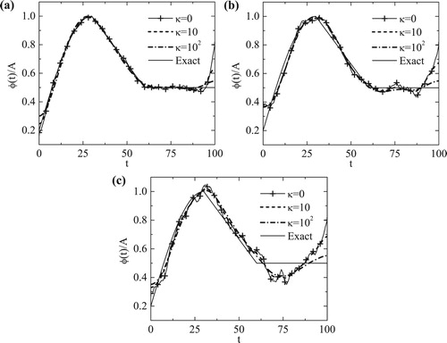
Figure 2. (a) The normalized objective functionalal $\overline{J}\left[{\phi }^n\right]$, (b) the normalized accuracy error $\overline{E}\left[{\phi }^n\right]$, and (c) numerical solutions of $\phi \left(t\right)$ with initial guess ${\phi }^0\left(t\right)=0.5A$ and $\kappa =1$, for noise $p\in \{0,1,3\}$, for Example 1.

Figure 3. Numerical solutions of $\phi \left(t\right)$ for various values of the smoothing parameter $\kappa \in \{0,10,{10}^2\}$, with initial guess ${\phi }^0\left(t\right)=0.8A$, for (a) p=0, (b) p=1 and (c) p=3 noise, for Example 1.

Example 2

We take the following input data: (42) $\begin{array}{ll}{k}_1=54\mathrm{W}/\left(\mathrm{m}{}^{\circ }\mathrm{C}\right),& k_2\left(x\right)=50{\mathrm{e}}^{100(x-0.005)}\mathrm{W}/\left(\mathrm{m}{}^{\circ }\mathrm{C}\right)\\ C_1=3.66\times {10}^6\mathrm{J}/\left({\mathrm{m}}^3{}^{\circ }\mathrm{C}\right),& C_2\left(x\right)=5\times {10}^6\times {\mathrm{e}}^{-50(x-0.005)}\mathrm{J}/\left({\mathrm{m}}^3{}^{\circ }\mathrm{C}\right)\\ T=80\mathrm{s},& L=0.02\mathrm{m},x_c=0.005\mathrm{m},\\ a_1={30}^{\circ }\mathrm{C},& a_2={300}^{\circ }\mathrm{C},\\ q_1=0,& q_2=-2\times {10}^5{\mathrm{W}/\mathrm{m}}^2.\end{array}$(42) Here, the bi-material $\mathrm{\Omega }={\mathrm{\Omega }}_1\cup {\mathrm{\Omega }}_2$ has a homogeneous component ${\mathrm{\Omega }}_1$ (as in Example 1), but the second component ${\mathrm{\Omega }}_2$ is an inhomogeneous material with spacewise dependent thermal properties $k_2\left(x\right)$ and $C_2\left(x\right)$. The inhomogeneous component ${\mathrm{\Omega }}_2$ is heated by a non-zero heat flux $q_2$. The heat diffusion from ${\mathrm{\Omega }}_2$ to ${\mathrm{\Omega }}_1$ is blocked by the thermal resistance at the imperfect interface $x=x_c$, which is characterised by a TCC. In this example, the boundary temperature at x=0 measured over time is used as input data to recover the temporal history of the unknown TCC. As accurate reconstruction of non-smooth and discontinuous functions is numerically challenging, we take the exact solution for $\phi \left(t\right)$ as (43) ${\phi }^{\star }\left(t\right)=\left\{\begin{array}{ll}0.2A,& t\in [0,40)\mathrm{s},\\ A,& t\in [40,80]\mathrm{s},\end{array}\right.$(43) where the scaling constant $A=5\times {10}^2$ W/(m² ${}^{\circ }$C). Note that the jump of ${\phi }^{\star }$ at $t=40\mathrm{s}$ in (43(43) ${\phi }^{\star }\left(t\right)=\left\{\begin{array}{ll}0.2A,& t\in [0,40)\mathrm{s},\\ A,& t\in [40,80]\mathrm{s},\end{array}\right.$(43) ) can be physically induced by a sudden change of an external load [21].

We take the arbitrary initial guess ${\phi }^0\left(t\right)=0.6A$. In the FDM scheme, we take $N_x=102$, $N_t=101$ and $N_c=26$. Figure 4 illustrates the evolutions of the normalized objective functional $\overline{J}\left[{\phi }^n\right]$ and the accuracy error $\overline{E}\left[{\phi }^n\right]$, as functions of the number of iterations n. As shown in Figure 4(a), when $\kappa =0$, the stopping criterion defined by the discrepancy principle (35(35) $J\left[{\phi }^k\right]\le \mathcal{E},$(35) ) is reached at $n_s\in \{6,6\}$ iterations for $p\in \{3,5\}$ noise, respectively. Besides, when $\kappa ={10}^3$, the corresponding stopping iteration numbers $n_s\in \{23,21\}$ are obtained in Figure 4(b). The first remark is that it takes more iterations to satisfy the stopping criterion for $\kappa ={10}^3$ than for $\kappa =0$. Although not illustrated, we report that on testing with other values of κ such as 1, 10 and ${10}^2$, the same conclusion that the number of stopping iterations $n_s$ increases monotonically with increasing κ has been confirmed. On the other hand, as shown in Figure 4(c,d), the increase in the noise level p leads to a dramatical increase of the accuracy error $\overline{E}\left[{\phi }^n\right]$ for $\kappa =0$, while this does not make any difference to the evolution of $\overline{E}\left[{\phi }^n\right]$ for $\kappa ={10}^3$. Thus, at the cost of slightly decreasing computational efficiency, the robustness of the iterative CGM with respect to the measurement noise is remarkably improved by smoothing the gradient $J_L^{\mathrm{\prime }}$ with a positive smoothing parameter κ.

Figure 4. The normalized objective functionalal $\overline{J}\left[{\phi }^n\right]$ for (a) $\kappa =0$ and (b) $\kappa ={10}^3$, and the normalized accuracy error $\overline{E}\left[{\phi }^n\right]$ for (c) $\kappa =0$ and (d) $\kappa ={10}^3$, for $p\in \{0,3,5\}$ noise, for Example 2.

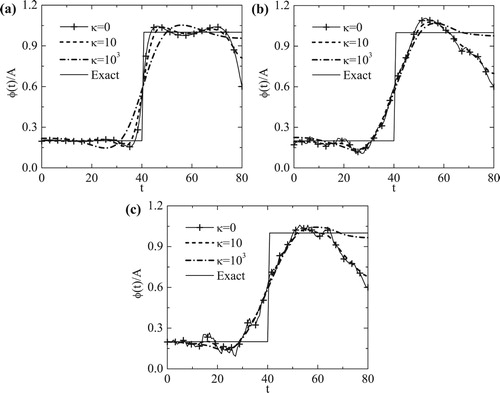
The effect of κ on the accuracy of the estimation of $\phi \left(t\right)$ is further studied. The variation of the normalized accuracy error $\overline{E}\left[{\phi }^n\right]$, at the stopping iteration numbers $n_s\in \{30,23,21\}$ for $p\in \{0,3,5\}$ noise, respectively, as a function of κ, is plotted in Figure 5. Note that the preconditioner M is close to the identity I for small values of κ. Hence, the preconditioner will play a critical role only if κ is not small. Figure 5 shows that $\overline{E}\left[{\phi }^n\right]$ keeps almost constant when $\log \left(\kappa \right)<1$. For $\log \left(\kappa \right)>1$, $\overline{E}\left[{\phi }^n\right]$ decreases as κ increases for $p\in \{3,5\}$, whilst an opposite trend is observed for p=0. It makes sense to compare the numerical solutions obtained using various values of κ. First, from Figure 6(b,c), for p=3 and p=5, respectively, it can be seen that the deviation in the numerical solution from its exact value near $t=T=80\mathrm{s}$ is avoided by increasing κ. This is the reason for the decrease of $\overline{E}\left[{\phi }^n\right]$ when $p\in \{3,5\}$. By contrast, Figure 6(a) reveals that the reconstruction of solution at the discontinuity point at $t=40\mathrm{s}$ becomes worse for larger κ because of the over-smoothness effect of the preconditioner. Thus, for exact data p=0, as we do not employ any regularization but stop the iterations at an arbitrary number, say after 30 iterations, $\overline{E}\left[{\phi }^n\right]$ is expected to increase with increasing κ for the discontinuous solution (43(43) ${\phi }^{\star }\left(t\right)=\left\{\begin{array}{ll}0.2A,& t\in [0,40)\mathrm{s},\\ A,& t\in [40,80]\mathrm{s},\end{array}\right.$(43) ).

Figure 5. Variation of the normalized accuracy error $\overline{E}\left[{\phi }^n\right]$, at the stopping iteration number $n_s$, with respect to κ, for $p\in \{0,3,5\}$ noise, for Example 2.

Figure 6. Retrieved solutions using various values of κ for (a) p=0, (b) p=3 and (c) p=5 noise, for Example 2.

4.2. 2D case for finding the space- and time-dependent interface coefficient

In this section, the numerical feasibility of the methodology for 2D inverse problems will be demonstrated to reconstruct the space and time variation of the interface coefficient. No a priori information is given on the distribution of the unknown function. The direct problem, sensitivity problem and adjoint problem are solved by the alternating-direction implicit (ADI) method [40] (see section A.2 of Appendix A).

Example 3

We take the following input data: (44) $\begin{array}{ll}{k}_1=54\mathrm{W}/(\mathrm{m}{}^{\circ }\mathrm{C}),& k_2=213\mathrm{W}/(\mathrm{m}{}^{\circ }\mathrm{C})\\ C_1=3.66\times {10}^6{\mathrm{J}/(\mathrm{m}}^3{}^{\circ }\mathrm{C}),& C_2=3.27\times {10}^6{\mathrm{J}/(\mathrm{m}}^3{}^{\circ }\mathrm{C})\\ T=20\mathrm{s},& L_x=L_y=0.1\mathrm{m},x_c=0.01\mathrm{m},\\ a_1={30}^{\circ }\mathrm{C},& a_2={900}^{\circ }\mathrm{C},\\ q_1=q_2=0,\end{array}$(44) where $k_1$ and $C_1$ correspond to the thermal properties of AISI 1050 steel [20], whilst $k_2$ and $C_2$ correspond to the material considered in [1] for determining the unknown TCC during metal casting. Both of the two space domains ${\mathrm{\Omega }}_1$ and ${\mathrm{\Omega }}_2$ are rectangular, with ${\mathrm{\Omega }}_1=(0,x_c)\times (0,L_y)$ and ${\mathrm{\Omega }}_2=(x_c,L_x)\times (0,L_y)$, where $L_x$ and $L_y$ are the lengths of the rectangular domain in x and y-directions, respectively, corresponding to the physical situation where the bi-material is segmented at the vertical interface $x=x_c$ along the y-axis with $y\in (0,L_y)$. The two components are both homogeneous and possess different thermal properties. The boundaries $\mathrm{\partial }{\mathrm{\Omega }}_1\mathrm{\setminus \Gamma }$ and $\mathrm{\partial }{\mathrm{\Omega }}_2\mathrm{\setminus \Gamma }$ are kept insulated. At the interface $\mathrm{\Gamma }=\left\{x_c\right\}\times (0,L_y)$, for the linear law $f\left(u\right)=u$, the unknown interface coefficient $\phi (y,t)$ represents a TCC, which is time-dependent and varies along the y-direction.

The exact solution ${\phi }^{\star }$ of the TCC is taken as (45) ${\phi }^{\star }(y,t)=0.5A\frac{y}{L_y}+0.5A\frac{t}{T}+0.1A,(y,t)\in [0,L_y]\times [0,T],$(45) with the scaling constant $A=1\times {10}^3{\mathrm{W}/(\mathrm{m}}^2{}^{\circ }\mathrm{C})$, which corresponds to a physical linear variation in space y and time t variables. We assume that the input temperature measurements (5(5) $u_1({\mathbf{x}}_i,t)=Y({\mathbf{x}}_i,t),({\mathbf{x}}_i,t)\in {\mathrm{\Gamma }}_0\times (0,T),i=\overline{1,N_m},$(5) ) are extracted from $N_m$ points of the thermal images of the boundary ${\mathrm{\Gamma }}_0=\left\{0\right\}\times [0,L_y]$, uniformly distributed with a step size $D_m=L_y/(N_m-1)$, $N_m\ge 2$.

We take the initial guess as ${\phi }^0(y,t)=0.4A$, the numbers of ADI nodes as $N_x=102$, $N_y=41$ and $N_t=101$, and the number of measurement points as $N_m=10$. Firstly, the preconditioned CGM with $\kappa =1$ is used to validate the algorithm for the 2D problem. Similar to the 1D case, a monotonic decreasing convergence of the normalized objective functional (38(38) $\begin{array}{rl}\overline{J}\left[{\phi }^n\right]& =\frac{\sum _{i=1}^{N_m}\parallel u_1({\mathbf{x}}_i,t;{\phi }^n)-Y({\mathbf{x}}_i,t){\parallel }_{L^2(0,T)}^2}{2\sum _{i=1}^{N_m}\parallel Y({\mathbf{x}}_i,t){\parallel }_{L^2(0,T)}^2},\end{array}$(38) ) is achieved. As shown in Figure 7(a), converged solutions are reached within 40 iterations for various noise levels $p\in \{0,3,5\}$, and the limit of $\overline{J}\left[{\phi }^n\right]$ increases with increasing p. When the input data contains $p\in \{3,5\}$ noise, the iterations are stopped, according to the discrepancy principle (35(35) $J\left[{\phi }^k\right]\le \mathcal{E},$(35) ) at $n_s\in \{11,10\}$, respectively. Figure 7(b) shows the corresponding normalized accuracy error $\overline{E}\left[{\phi }^n\right]$, from which the optimal iteration numbers are determined as $n_{\mathrm{opt}}=18$ for both noise levels $p\in \{3,5\}$. Although there is a difference between the numbers $n_s$ and $n_{\mathrm{opt}}$, the value of $\overline{E}\left[{\phi }^n\right]$ at $n_s$ is very close to that at $n_{\mathrm{opt}}$. Moreover, the divergence of $\overline{E}\left[{\phi }^n\right]$ illustrated in Figure 7(b), is much less pronounced than that shown in Figures 2(b) and 4(c) for Examples 1 and 2, respectively.

Figure 7. (a) The normalized objective functionalal $\overline{J}\left[{\phi }^n\right]$ and (b) the normalized accuracy error $\overline{E}\left[{\phi }^n\right]$ for $\kappa =1$, for $p\in \{0,3,5\}$ noise, for Example 3.

We also analyse in Figure 8, the variation of the normalized accuracy error $\overline{E}\left[{\phi }^n\right]$, as a function of the smoothing parameter κ, for various noise levels. The numerical solutions are obtained after 40 iterations for noiseless data, and $n_s$ iterations for noisy data, where $n_s$ is determined from discrepancy principle (35(35) $J\left[{\phi }^k\right]\le \mathcal{E},$(35) ). It can been remarked from Figure 8 that $\overline{E}\left[{\phi }^n\right]$ decreases, as κ increases, for all noise levels $p\in \{0,3,5\}$. However, we have found that for too large κ, such as $\log \left(\kappa \right)>2$, the discrepancy principle oversmoothes the numerical solution by enforcing it to be too stable but inaccurate. In view of the satisfactory accuracy, the preconditioned CGM with $\kappa ={10}^2$ will be used below to compare the results with the standard CGM.

Figure 8. The variation of the normalized accuracy error $\overline{E}\left[{\phi }^n\right]$ with the smoothing parameter κ, for $p\in \{0,3,5\}$ noise, for Example 3.

Figure 9 shows the comparisons between the exact solution (45(45) ${\phi }^{\star }(y,t)=0.5A\frac{y}{L_y}+0.5A\frac{t}{T}+0.1A,(y,t)\in [0,L_y]\times [0,T],$(45) ) of $\phi (y,t)$ and the recovered solutions obtained with $\kappa =0$ and $\kappa ={10}^2$, when noiseless data (p=0) is inverted. The inaccuracies near $t=20\mathrm{s}$ in Figure 9(b) are caused by the vanishing of $L^2$-gradient $J_L^{\mathrm{\prime }}$ at the final time, which fails to move the boundary values from the initial guess. Fortunately, these inaccuracies can be overcome by employing the preconditioned CGM with $\kappa ={10}^2$, as shown in Figure 9(c).

Figure 9. (a) The exact $\phi (y,t)$ given by (45(45) ${\phi }^{\star }(y,t)=0.5A\frac{y}{L_y}+0.5A\frac{t}{T}+0.1A,(y,t)\in [0,L_y]\times [0,T],$(45) ) and the numerical solutions obtained with (b) $\kappa =0$ and (c) $\kappa ={10}^2$ after 40 iterations, for exact data (p=0), for Example 3.

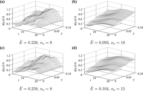
For noisy input data ($p\in \{3,5\}$), the retrieved solutions for $\kappa =0$ and $\kappa ={10}^2$ are illustrated in Figure 10. Besides the improvement of accuracy near the final time, the oscillations in the numerical solutions (Figure 10(a,c)) are smoothed considerably (Figure 10(b,d)) by using the preconditioned CGM with $\kappa ={10}^2$, in comparison with the solutions obtained by standard CGM with $\kappa =0$. This is the reason for the decrease of $\overline{E}\left[{\phi }^n\right]$ shown in Figure 8. Hence, for an arbitrary initial guess, the preconditioned CGM is able to retrieve the coefficient $\phi (y,t)$ accurately and stably.

Figure 10. The numerical solutions of $\phi (y,t)$ for p=3 noise: (a) $\kappa =0$, (b) $\kappa ={10}^2$, and for p=5 noise: (c) $\kappa =0$, (d) $\kappa ={10}^2$, for Example 3.

In practice, the number $N_m$ of measurement points on ${\mathrm{\Gamma }}_0=\left\{0\right\}\times [0,L_y]$ is important for experiment design, due to its effect on the accuracy of the recovery of unknown interfacial coefficient $\phi (y,t)$. Figure 11 shows the normalized accuracy error $\overline{E}\left[{\phi }^n\right]$, at the corresponding stopping iteration numbers, as a function of the number of measurement points $N_m$ for $\kappa \in \{0,{10}^2\}$ and p=5 noise. From this figure, it can be seen that the errors for $\kappa ={10}^2$ are smaller than those for $\kappa =0$, for all values of $N_m$, which is in accordance with the results presented in Figure 8. The error $\overline{E}\left[{\phi }^n\right]$ is first decreasing rapidly, followed by a slight variation around a certain value as $N_m$ increases. An optimal number $N_{mc}$ is obtained, in this example we have $N_{mc}=6$, which is the minimum number of boundary temperature measurements at x=0 for obtaining an inverse solution with attainable accuracy for noisy data. Also, from the numerical point of view, for $N_m\ge N_{mc}$, increasing $N_m$ will have little effect on the accuracy.

Figure 11. The variation of the normalized accuracy error $\overline{E}\left[{\phi }^n\right]$, at the corresponding stopping iteration numbers, with the number of measurement points $N_m$, for $\kappa \in \{0,{10}^2\}$ and p=5 noise, for Example 3.

Example 4

We take the same input data (44(44) $\begin{array}{ll}{k}_1=54\mathrm{W}/(\mathrm{m}{}^{\circ }\mathrm{C}),& k_2=213\mathrm{W}/(\mathrm{m}{}^{\circ }\mathrm{C})\\ C_1=3.66\times {10}^6{\mathrm{J}/(\mathrm{m}}^3{}^{\circ }\mathrm{C}),& C_2=3.27\times {10}^6{\mathrm{J}/(\mathrm{m}}^3{}^{\circ }\mathrm{C})\\ T=20\mathrm{s},& L_x=L_y=0.1\mathrm{m},x_c=0.01\mathrm{m},\\ a_1={30}^{\circ }\mathrm{C},& a_2={900}^{\circ }\mathrm{C},\\ q_1=q_2=0,\end{array}$(44) ) as in Example 3, but the heat transfer at the interface $\mathrm{\Gamma }=\left\{x_c\right\}\times (0,L_y)$ is governed by a Stefan-Boltzmann radiation condition with unknown SBC, $\phi (y,t)$. Thus we have $f\left(u\right)=u^4$ and the exact solution of $\phi (y,t)$ is given by (46) ${\phi }^{\star }(y,t)=0.5A\cdot \sin \left(\frac{2\pi y}{L_y}\right)+A,(y,t)\in [0,L_y]\times [0,T],$(46) where the scaling constant $A=1\times {10}^{-7}{\mathrm{W}/(\mathrm{m}}^2{}^{\circ }{\mathrm{C}}^4)$, which corresponds to a physical harmonic oscillatory variation in the space variable y.

The initial guess is taken as ${\phi }^0(y,t)=0.4A$, which is far from the analytical solution at the final time $t=T=20\mathrm{s}$, to see further the merits of the preconditioned CGM over its standard version. We take the numbers of nodes $N_x=102$, $N_y=41$ and $N_t=101$, and the number of measurement points $N_m=10$. To determine the appropriate value of the smoothing parameter κ, the evolution of $\overline{E}\left[{\phi }^n\right]$, as a function of κ, is plotted in Figure 12, where $\overline{E}\left[{\phi }^n\right]$ is obtained after 30 iterations for p=0 and $n_s$ iterations for $p\in \{3,5\}$ noise. The figure reveals that an improvement in accuracy is achieved by increasing κ. We also find that the discrepancy principle fails to stop the iteration properly when $\log \left(\kappa \right)>3$ in this example. For this reason, the preconditioned CGM with $\kappa ={10}^3$ will be used below for the retrieval of $\phi (y,t)$.

Figure 12. The variation of the normalized accuracy error $\overline{E}\left[{\phi }^n\right]$ with the smoothing parameter κ, for $p\in \{0,3,5\}$ noise, for Example 4.

For noiseless data, the retrieved solutions of $\phi (y,t)$ obtained by the standard and the preconditioned CGM with $\kappa ={10}^3$ are shown in Figure 13(b,c), respectively. By comparing with the analytical solution (46(46) ${\phi }^{\star }(y,t)=0.5A\cdot \sin \left(\frac{2\pi y}{L_y}\right)+A,(y,t)\in [0,L_y]\times [0,T],$(46) ) in Figure 13(a), it can be seen that the solution given by the preconditioned CGM is in good agreement with the analytical one, while the solution given by the standard CGM does not move from the initial guess at $t=20\mathrm{s}$. Thus the retrieval of $\phi (y,t)$ by preconditioned CGM possesses a higher accuracy than that by standard CGM also for nonlinear problem.

Figure 13. (a) The exact $\phi (y,t)$ given by (46(46) ${\phi }^{\star }(y,t)=0.5A\cdot \sin \left(\frac{2\pi y}{L_y}\right)+A,(y,t)\in [0,L_y]\times [0,T],$(46) ) and the numerical solutions obtained with (b) $\kappa =0$ and (c) $\kappa ={10}^3$ after 30 iterations, for exact data (p=0), for Example 4.

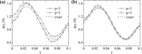
For noisy data ($p\in \{3,5\}$), Figure 14 shows the retrieved solutions of $\phi (y,t)$ obtained after $n_s$ iterations, determined by the discrepancy principle (35(35) $J\left[{\phi }^k\right]\le \mathcal{E},$(35) ). Figure 15 further shows the corresponding solutions in y-direction at $t=0.5T=10\mathrm{s}$. From Figures 14 and 15, one can notice that the oscillations induced by the noise in the input temperature data are removed substantially by using the preconditioned CGM with $\kappa ={10}^3$. The inaccuracies occurring near the final time are corrected and the deviations from the exact solution along the space boundary are also reduced. In addition, the error $\overline{E}\left[{\phi }^n\right]$ are almost the same for $\kappa ={10}^3$ regardless of the noise level, as shown in Figures 12 and 14, and this adds further robustness to the preconditioned CGM that was successfully developed and employed in this paper.

Figure 14. The numerical solutions of $\phi (y,t)$ for p=3 noise: (a) $\kappa =0$, (b) $\kappa ={10}^3$, and for p=5 noise: (c) $\kappa =0$, (d) $\kappa ={10}^3$, after $n_s$ iterations, for Example 4.

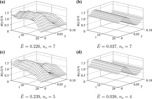
Figure 15. The exact and numerical solutions of $\phi (y,10)$ for (a) $\kappa =0$ and (b) $\kappa ={10}^3$ after $n_s$ iterations, for $p\in \{3,5\}$ noise, for Example 4.

5. Conclusions

A stable and robust preconditioned CGM with adjoint problem has been implemented for the reconstruction of space and time varying interface heat transfer coefficient φ (both linear TCC and nonlinear SBC) from temperature measurements on an accessible portion of the boundary. The numerical procedure is applied to both 1D and 2D problems with various evolutions of $\phi \left(t\right)$ and $\phi (y,t)$, respectively. The numerical results have revealed that both the discrepancy principle and the preconditioner $M=(I-\kappa {\mathrm{\nabla }}_t^2)$ have regularizing effects on the retrieved solution of the unknown interface coefficient φ. It was demonstrated that, in comparison with the standard CGM, the preconditioned CGM developed in this article achieves better accuracy and stability even for relatively high noise levels in the measurement data and arbitrary initial guesses of the iterative procedure. For noisy data, the accuracy improves as the smoothing parameter κ in the preconditioner M increases. In the 1D case, due to the over-smoothness of the preconditioner M, the reconstruction of discontinuities in the evolution of φ is less accurate than that on the continuous portions, but is still reasonably stable. Besides, in the 2D case, there exists an optimal number $N_{mc}$ of measurement points, beyond which increasing it will make little contribution to the improvement of accuracy. The rigorous choice of the smoothing parameter κ in (30(30) $J_H^{\mathrm{\prime }}-\kappa \frac{{\mathrm{\partial }}^2{J}_H^{\mathrm{\prime }}}{\mathrm{\partial }{t}^2}=J_L^{\mathrm{\prime }}\mathrm{on}{S}_T.$(30) ) is still open to further investigations and, at this stage, represents a limitation of the presented method.

Extensions to multilayer materials and three-dimensional computations are straightforward. Also, in the future, for validation purpose, the accuracy, stability and robustness of the proposed preconditioned CGM, that have been verified in this study, should be tested on inverting real raw data in order to completely validate the inverse model for reconstructing the interfacial heat transfer coefficient in composite materials.

Disclosure statement

No potential conflict of interest was reported by the authors.

Additional information

Funding

This work was supported by the National Natural Science Foundation of China under [grant number 11502058]; and the National Basic Research Program of China (or 973 Program) under [grant number 2015CB655200]. The first author would like to acknowledge the financial support from the China Scholarship Council (CSC).

Appendix. Numerical schemes of direct problem

A.1 1D transient heat conduction

A uniform mesh is constructed for numerical discretization, with the nodes and mesh sizes as follows: (A1) $\begin{array}{l}{x}_i=(i-1)\delta x,\mathrm{for}i=\overline{1,N_c},\mathrm{and}\\ x_i=(i-2)\delta x,\mathrm{for}i=\overline{N_c+1,N_x},\delta x=L/(N_x-2),\\ t_m=(m-1)\delta t,\delta t=T/(N_t-1),m=\overline{1,N_t},\end{array}$(A1) where $x_i$ and $t_m$ are the nodes in space and time domain, respectively, and $\delta x$ and $\delta t$ are the corresponding mesh sizes. The location of the interface is at $x_c=x_{N_c}=x_{N_c+1}=(N_c-1)\delta x$.

For convenience, the temperatures $u_1$ and $u_2$ in Eqs. (1(1) $C_i\left(\mathbf{x}\right)\frac{\mathrm{\partial }{u}_i}{\mathrm{\partial }t}=\mathrm{\nabla }\cdot \left(k_i\right(\mathbf{x}\left)\mathrm{\nabla }{u}_i\right),(\mathbf{x},t)\in {\mathrm{\Omega }}_i\times (0,T),i=1,2$(1) )–(4(4) $u_i(\mathbf{x},0)=a_i\left(\mathbf{x}\right),\mathbf{x}\in {\mathrm{\Omega }}_i,i=1,2,$(4) ) are denoted by a single variable w next. By employing an implicit FDM scheme, the discretized form of Eq. (1(1) $C_i\left(\mathbf{x}\right)\frac{\mathrm{\partial }{u}_i}{\mathrm{\partial }t}=\mathrm{\nabla }\cdot \left(k_i\right(\mathbf{x}\left)\mathrm{\nabla }{u}_i\right),(\mathbf{x},t)\in {\mathrm{\Omega }}_i\times (0,T),i=1,2$(1) ) is (A2) $C_{l,i}\frac{w_i^{m+1}-w_i^m}{\delta t}=\frac{k_{l,i+1/2}}{(\delta x{)}^2}{w}_{i+1}^{m+1}-\frac{k_{l,i+1/2}+k_{l,i-1/2}}{(\delta x{)}^2}{w}_i^{m+1}+\frac{k_{l,i-1/2}}{(\delta x{)}^2}{w}_{i-1}^{m+1},$(A2) where l=1,2, $m=\overline{1,N_t-1}$, $i=\overline{1,N_c}$ for l=1, $i=\overline{N_c+1,N_x}$ for l=2, $k_{l,i}$ and $C_{l,i}$ are thermal conductivity and heat capacity per unit volume of ${\mathrm{\Omega }}_l$ at $x_i$, respectively, $k_{l,i\pm 1/2}=(k_{l,i}+k_{l,i\pm 1})/2$, and $w_i^m$ denotes the nodal temperature at position $x_i$ and time $t_m$. When i=1 or $i=N_x$ in (A2(A2) $C_{l,i}\frac{w_i^{m+1}-w_i^m}{\delta t}=\frac{k_{l,i+1/2}}{(\delta x{)}^2}{w}_{i+1}^{m+1}-\frac{k_{l,i+1/2}+k_{l,i-1/2}}{(\delta x{)}^2}{w}_i^{m+1}+\frac{k_{l,i-1/2}}{(\delta x{)}^2}{w}_{i-1}^{m+1},$(A2) ), $w_0^{m+1}$ and $w_{N_x+1}^{m+1}$ are nodal temperatures at fictitious points i=0 and $N_x+1$ on the left-hand side and right-hand side of the boundaries x=0 and x=L, respectively.

In order to approximate the interface condition (3(3) $-k_1\left(\mathbf{x}\right)\frac{\mathrm{\partial }{u}_1}{\mathrm{\partial }{n}_1}=k_2\left(\mathbf{x}\right)\frac{\mathrm{\partial }{u}_2}{\mathrm{\partial }{n}_2}=\phi (\mathbf{x},t)\left[f\right(u_1)-f(u_2\left)\right],(\mathbf{x},t)\in \mathrm{\Gamma }\times (0,T),$(3) ), the nonlinear function f is linearized by a first-order Taylor series expansion, (A3) $f\left(w_i^{m+1}\right)=f\left(w_i^m\right)+f^{\mathrm{\prime }}\left(w_i^m\right)(w_i^{m+1}-w_i^m).$(A3) By using Eq. (A3(A3) $f\left(w_i^{m+1}\right)=f\left(w_i^m\right)+f^{\mathrm{\prime }}\left(w_i^m\right)(w_i^{m+1}-w_i^m).$(A3) ), one can discretize the interface condition (3(3) $-k_1\left(\mathbf{x}\right)\frac{\mathrm{\partial }{u}_1}{\mathrm{\partial }{n}_1}=k_2\left(\mathbf{x}\right)\frac{\mathrm{\partial }{u}_2}{\mathrm{\partial }{n}_2}=\phi (\mathbf{x},t)\left[f\right(u_1)-f(u_2\left)\right],(\mathbf{x},t)\in \mathrm{\Gamma }\times (0,T),$(3) ) into the following two recurrence relationships: (A4) $\begin{array}{rl}& -2r_1{w}_{N_c-1}^{m+1}+\left[1+2r_1+\frac{2r_1\delta x{\phi }^{m+1}}{k_{1,N_c}}{f}^{\mathrm{\prime }}\left(w_{N_c}^m\right)\right]w_{N_c}^{m+1}\\ & -\frac{2r_1\delta x{\phi }^{m+1}}{k_{1,N_c}}{f}^{\mathrm{\prime }}\left(w_{N_c+1}^m\right)w_{N_c+1}^{m+1}=w_{N_c}^m-\frac{2r_1\delta x{F}^m}{k_{1,N_c}},m=\overline{1,N_t-1},\end{array}$(A4) (A5) $\begin{array}{rl}& -2r_2{w}_{N_c+2}^{m+1}+\left[1+2r_2+\frac{2r_2\delta x{\phi }^{m+1}}{k_{2,N_c+1}}{f}^{\mathrm{\prime }}\left(w_{N_c+1}^m\right)\right]w_{N_c+1}^{m+1}\\ & -\frac{2r_2\delta x{\phi }^{m+1}}{k_{2,N_c+1}}{f}^{\mathrm{\prime }}\left(w_{N_c}^m\right)w_{N_c}^{m+1}=w_{N_c+1}^m+\frac{2r_2\delta x{F}^m}{k_{2,N_c+1}},m=\overline{1,N_t-1},\end{array}$(A5) corresponding to the domain ${\mathrm{\Omega }}_1$ and ${\mathrm{\Omega }}_2$, respectively, where, (A6) $r_1=\frac{k_{1,N_c-1/2}}{C_{1,N_c}}\cdot \frac{\delta t}{(\delta x{)}^2},r_2=\frac{k_{2,N_c+3/2}}{C_{2,N_c+1}}\cdot \frac{\delta t}{(\delta x{)}^2},$(A6) and (A7) $F^m={\phi }^{m+1}\left[f\right(w_{N_c}^m)-f(w_{N_c+1}^m\left)\right]+{\phi }^{m+1}\left[f^{\mathrm{\prime }}\right(w_{N_c+1}^m)w_{N_c+1}^m-f^{\mathrm{\prime }}(w_{N_c}^m\left)w_{N_c}^m\right].$(A7) Here, the approximations, $k_{1,N_c+1/2}=k_{1,N_c-1/2}$ and $k_{2,N_c+1/2}=k_{2,N_c+3/2}$, are made in Eqs.(A4(A4) $\begin{array}{rl}& -2r_1{w}_{N_c-1}^{m+1}+\left[1+2r_1+\frac{2r_1\delta x{\phi }^{m+1}}{k_{1,N_c}}{f}^{\mathrm{\prime }}\left(w_{N_c}^m\right)\right]w_{N_c}^{m+1}\\ & -\frac{2r_1\delta x{\phi }^{m+1}}{k_{1,N_c}}{f}^{\mathrm{\prime }}\left(w_{N_c+1}^m\right)w_{N_c+1}^{m+1}=w_{N_c}^m-\frac{2r_1\delta x{F}^m}{k_{1,N_c}},m=\overline{1,N_t-1},\end{array}$(A4) ) and (A5(A5) $\begin{array}{rl}& -2r_2{w}_{N_c+2}^{m+1}+\left[1+2r_2+\frac{2r_2\delta x{\phi }^{m+1}}{k_{2,N_c+1}}{f}^{\mathrm{\prime }}\left(w_{N_c+1}^m\right)\right]w_{N_c+1}^{m+1}\\ & -\frac{2r_2\delta x{\phi }^{m+1}}{k_{2,N_c+1}}{f}^{\mathrm{\prime }}\left(w_{N_c}^m\right)w_{N_c}^{m+1}=w_{N_c+1}^m+\frac{2r_2\delta x{F}^m}{k_{2,N_c+1}},m=\overline{1,N_t-1},\end{array}$(A5) ). The Neumann boundary condition (2(2) $-k_i\left(\mathbf{x}\right)\frac{\mathrm{\partial }{u}_i}{\mathrm{\partial }{n}_i}=q_i(\mathbf{x},t),(\mathbf{x},t)\in {\mathrm{\Gamma }}_i\times (0,T),i=1,2$(2) ) is discretized as follows: (A8) $k_{1,1}\frac{w_0^{m+1}-w_2^{m+1}}{2\delta x}=q_1^{m+1},k_{2,N_x}\frac{w_{N_x-1}^{m+1}-w_{N_x+1}^{m+1}}{2\delta x}=q_2^{m+1},m=\overline{1,N_t-1},$(A8) By substituting Eq. (A8(A8) $k_{1,1}\frac{w_0^{m+1}-w_2^{m+1}}{2\delta x}=q_1^{m+1},k_{2,N_x}\frac{w_{N_x-1}^{m+1}-w_{N_x+1}^{m+1}}{2\delta x}=q_2^{m+1},m=\overline{1,N_t-1},$(A8) ) into Eq. (A2(A2) $C_{l,i}\frac{w_i^{m+1}-w_i^m}{\delta t}=\frac{k_{l,i+1/2}}{(\delta x{)}^2}{w}_{i+1}^{m+1}-\frac{k_{l,i+1/2}+k_{l,i-1/2}}{(\delta x{)}^2}{w}_i^{m+1}+\frac{k_{l,i-1/2}}{(\delta x{)}^2}{w}_{i-1}^{m+1},$(A2) ), the fictitious nodal temperatures can be eliminated. Thus, the direct problem (1(1) $C_i\left(\mathbf{x}\right)\frac{\mathrm{\partial }{u}_i}{\mathrm{\partial }t}=\mathrm{\nabla }\cdot \left(k_i\right(\mathbf{x}\left)\mathrm{\nabla }{u}_i\right),(\mathbf{x},t)\in {\mathrm{\Omega }}_i\times (0,T),i=1,2$(1) )-(4(4) $u_i(\mathbf{x},0)=a_i\left(\mathbf{x}\right),\mathbf{x}\in {\mathrm{\Omega }}_i,i=1,2,$(4) ) is transformed into a series of systems of linear algebraic equations, which are solved using the Tridiagonal-Matrix algorithm (TDMA) [41].

A.2 2D transient heat conduction

The domain $\mathrm{\Omega }\times (0,T)$ is discretized into a uniform mesh of nodes and sizes as follows: (A9) $\begin{array}{l}{x}_i=(i-1)\delta x,\mathrm{for}i=\overline{1,N_c},\mathrm{and}\\ x_i=(i-2)\delta x,\mathrm{for}i=\overline{N_c+1,N_x},\delta x=L_x/(N_x-2),\\ y_j=(j-1)\delta y,\delta y=L_y/(N_y-1),j=\overline{1,N_y},\\ t_m=(m-1)\delta t,\delta t=T/(N_t-1),m=\overline{1,N_t},\end{array}$(A9) The alternating-direction implicit (ADI) method is used for the discretization of the heat equation (1(1) $C_i\left(\mathbf{x}\right)\frac{\mathrm{\partial }{u}_i}{\mathrm{\partial }t}=\mathrm{\nabla }\cdot \left(k_i\right(\mathbf{x}\left)\mathrm{\nabla }{u}_i\right),(\mathbf{x},t)\in {\mathrm{\Omega }}_i\times (0,T),i=1,2$(1) ) with constant thermal properties $k_i$ and $C_i$ (i=1,2), as follows: (A10) $\begin{array}{rl}{C}_l\frac{w_{i,j}^{2m+1}-w_{i,j}^{2m}}{\delta t}& =\frac{k_l}{(\delta x{)}^2}\left(w_{i-1,j}^{2m+1}-2w_{i,j}^{2m+1}+w_{i+1,j}^{2m+1}\right)\\ & +\frac{k_l}{(\delta y{)}^2}\left(w_{i,j-1}^{2m}-2w_{i,j}^{2m}+w_{i,j+1}^{2m}\right),l=1,2,\end{array}$(A10) (A11) $\begin{array}{rl}{C}_l\frac{w_{i,j}^{2m+2}-w_{i,j}^{2m+1}}{\delta t}& =\frac{k_l}{(\delta x{)}^2}\left(w_{i-1,j}^{2m+1}-2w_{i,j}^{2m+1}+w_{i+1,j}^{2m+1}\right)\\ & +\frac{k_l}{(\delta y{)}^2}\left(w_{i,j-1}^{2m+2}-2w_{i,j}^{2m+2}+w_{i,j+1}^{2m+2}\right),l=1,2,\end{array}$(A11) where $i=\overline{1,N_c}$ for l=1 and $i=\overline{N_c+1,N_x}$ for l=2, $j=\overline{1,N_y}$, $m=\overline{1/2,N_t/2-1}$, and $w_{i,j}^m$ denotes the nodal temperature at position $(x_i,y_j)$ and time $t_m$. Equations (A10(A10) $\begin{array}{rl}{C}_l\frac{w_{i,j}^{2m+1}-w_{i,j}^{2m}}{\delta t}& =\frac{k_l}{(\delta x{)}^2}\left(w_{i-1,j}^{2m+1}-2w_{i,j}^{2m+1}+w_{i+1,j}^{2m+1}\right)\\ & +\frac{k_l}{(\delta y{)}^2}\left(w_{i,j-1}^{2m}-2w_{i,j}^{2m}+w_{i,j+1}^{2m}\right),l=1,2,\end{array}$(A10) ) and (A11(A11) $\begin{array}{rl}{C}_l\frac{w_{i,j}^{2m+2}-w_{i,j}^{2m+1}}{\delta t}& =\frac{k_l}{(\delta x{)}^2}\left(w_{i-1,j}^{2m+1}-2w_{i,j}^{2m+1}+w_{i+1,j}^{2m+1}\right)\\ & +\frac{k_l}{(\delta y{)}^2}\left(w_{i,j-1}^{2m+2}-2w_{i,j}^{2m+2}+w_{i,j+1}^{2m+2}\right),l=1,2,\end{array}$(A11) ) can be further written into the following form suitable for calculation: (A12) $\begin{array}{rl}& (1+2r_{lx})w_{i,j}^{2m+1}-r_{lx}{w}_{i-1,j}^{2m+1}-r_{lx}{w}_{i+1,j}^{2m+1}=(1-2r_{ly})w_{i,j}^{2m}+r_{ly}{w}_{i,j-1}^{2m}+r_{ly}{w}_{i,j+1}^{2m},\end{array}$(A12) (A13) $\begin{array}{rl}& (1+2r_{ly})w_{i,j}^{2m+2}-r_{ly}{w}_{i,j-1}^{2m+2}-r_{ly}{w}_{i,j+1}^{2m+2}=(1-2r_{lx})w_{i,j}^{2m+1}+r_{lx}{w}_{i-1,j}^{2m+1}+r_{lx}{w}_{i+1,j}^{2m+1},\end{array}$(A13) where $r_{lx}=C_l\delta t/\left(k_l\right(\delta x{)}^2)$ and $r_{ly}=C_l\delta t/\left(k_l\right(\delta y{)}^2)$, l=1,2. For each specific m in the recurrences, Eq. (A12(A12) $\begin{array}{rl}& (1+2r_{lx})w_{i,j}^{2m+1}-r_{lx}{w}_{i-1,j}^{2m+1}-r_{lx}{w}_{i+1,j}^{2m+1}=(1-2r_{ly})w_{i,j}^{2m}+r_{ly}{w}_{i,j-1}^{2m}+r_{ly}{w}_{i,j+1}^{2m},\end{array}$(A12) ) is firstly solved to obtain the nodal temperatures at time $t_{2m+1}$, which are then substituted into Eq. (A13(A13) $\begin{array}{rl}& (1+2r_{ly})w_{i,j}^{2m+2}-r_{ly}{w}_{i,j-1}^{2m+2}-r_{ly}{w}_{i,j+1}^{2m+2}=(1-2r_{lx})w_{i,j}^{2m+1}+r_{lx}{w}_{i-1,j}^{2m+1}+r_{lx}{w}_{i+1,j}^{2m+1},\end{array}$(A13) ) to calculate the nodal temperatures at time $t_{2m+2}$.

When $i=N_c$ and $N_c+1$, the interface condition (3(3) $-k_1\left(\mathbf{x}\right)\frac{\mathrm{\partial }{u}_1}{\mathrm{\partial }{n}_1}=k_2\left(\mathbf{x}\right)\frac{\mathrm{\partial }{u}_2}{\mathrm{\partial }{n}_2}=\phi (\mathbf{x},t)\left[f\right(u_1)-f(u_2\left)\right],(\mathbf{x},t)\in \mathrm{\Gamma }\times (0,T),$(3) ) must be considered to obtain the following recurrences involving the interfacial nodal temperatures by using Eq. (A3(A3) $f\left(w_i^{m+1}\right)=f\left(w_i^m\right)+f^{\mathrm{\prime }}\left(w_i^m\right)(w_i^{m+1}-w_i^m).$(A3) ): (A14) $\begin{array}{r}{M}_1{w}_{N_c-1,j}^{2m+1}+M_2{w}_{N_c,j}^{2m+1}+M_3{w}_{N_c+1,j}^{2m+1}=(1-2r_{1y})w_{N_c,j}^{2m}+r_{1y}{w}_{N_c,j-1}^{2m}+r_{1y}{w}_{N_c,j+1}^{2m}-\frac{2\delta t}{\delta x{C}_1}P,\end{array}$(A14) (A15) $\begin{array}{r}{N}_3{w}_{N_c,j}^{2m+1}+N_2{w}_{N_c+1,j}^{2m+1}+N_1{w}_{N_c+2,j}^{2m+1}=(1-2r_{2y})w_{N_c+1,j}^{2m}+r_{2y}{w}_{N_c+1,j-1}^{2m}+r_{2y}{w}_{N_c+1,j+1}^{2m}+\frac{2\delta t}{\delta x{C}_2}P,\end{array}$(A15) (A16) $\begin{array}{r}(1+2r_{1y})w_{N_c,j}^{2m+2}-r_{1y}{w}_{N_c,j-1}^{2m+2}-r_{1y}{w}_{N_c,j+1}^{2m+2}=(1-2r_{1x})w_{N_c,j}^{2m+1}+2r_{1x}{w}_{N_c-1,j}^{2m+1}-\frac{2\delta t}{\delta x{C}_1}Q,\end{array}$(A16) (A17) $\begin{array}{r}(1+2r_{2y})w_{N_c+1,j}^{2m+2}-r_{2y}{w}_{N_c+1,j-1}^{2m+2}-r_{2y}{w}_{N_c+1,j+1}^{2m+2}=(1-2r_{2x})w_{N_c+1,j}^{2m+1}+2r_{2x}{w}_{N_c+2,j}^{2m+1}+\frac{2\delta t}{\delta x{C}_2}Q,\end{array}$(A17) where (A18) $\begin{array}{ll}{M}_1=-2r_{1x},& N_1=-2r_{2x}\\ M_2=1+2r_{1x}+\frac{2\delta t}{\delta x{C}_1}{\phi }_j^{2m+1}{f}^{\mathrm{\prime }}\left(w_{N_c,j}^{2m}\right),& N_2=1+2r_{2x}+\frac{2\delta t}{\delta x{C}_2}{\phi }_j^{2m+1}{f}^{\mathrm{\prime }}\left(w_{N_c+1,j}^{2m}\right)\\ M_3=-\frac{2\delta t}{\delta x{C}_1}{\phi }_j^{2m+1}{f}^{\mathrm{\prime }}\left(w_{N_c+1,j}^{2m}\right),& N_3=-\frac{2\delta t}{\delta x{C}_2}{\phi }_j^{2m+1}{f}^{\mathrm{\prime }}\left(w_{N_c,j}^{2m}\right)\end{array}$(A18) and (A19) $\begin{array}{rl}& P={\phi }_j^{2m+1}\left[f\right(w_{N_c,j}^{2m})-f(w_{N_c+1,j}^{2m})+f^{\mathrm{\prime }}(w_{N_c+1,j}^{2m})w_{N_c+1,j}^{2m}-f^{\mathrm{\prime }}(w_{N_c,j}^{2m}\left)w_{N_c,j}^{2m}\right],\\ & Q={\phi }_j^{2m+1}\left(f\right(w_{N_c,j}^{2m+1})-f(w_{N_c+1,j}^{2m+1}\left)\right).\end{array}$(A19) The boundary conditions are introduced in a similar manner as in the 1D case, and the resulting systems of algebraic equations are solved using the TDMA.

References

- Huang CH, Ozisik MN, Sawaf B. Conjugate gradient method for determining unknown contact conductance during metal casting. Int J Heat Mass Transf. 1992;35(7):1779–1786. doi: 10.1016/0017-9310(92)90148-L
- Yang G, Yamamoto M, Cheng J. Heat transfer in composite materials with Stefan–Boltzmann interface conditions. Math Methods Appl Sci. 2008;31(11):1297–1314. doi: 10.1002/mma.971
- Cheng J, Lu S, Yamamoto M. Reconstruction of the Stefan–Boltzmann coefficients in a heat-transfer process. Inverse Probl. 2012;28(4):045007. doi: 10.1088/0266-5611/28/4/045007
- Bermúdez A, Leira R, Muñiz MC, et al. Numerical modelling of a transient conductive–radiative thermal problem arising in silicon purification. Finite Elem Anal Des. 2006;42(10):809–820. doi: 10.1016/j.finel.2005.08.009
- Hu X, Xu X, Chen W. Numerical method for the inverse heat transfer problem in composite materials with Stefan-Boltzmann conditions. Adv Comput Math. 2010;33(4):471–489. doi: 10.1007/s10444-009-9131-x
- Ruan Y, Liu JC, Richmond O. Determining the unknown cooling condition and contact heat transfer coefficient during solidification of alloys. Inverse Probl Sci Eng. 1994;1(1):45–69. doi: 10.1080/174159794088027572
- Huang CH, Wang DM, Chen HM. Prediction of local thermal contact conductance in plate finned-tube heat exchangers. Inverse Probl Eng. 1999;7(2):119–141. doi: 10.1080/174159799088027690
- Caron EJFR, Daun KJ, Wells MA. Experimental heat transfer coefficient measurements during hot forming die quenching of boron steel at high temperatures. Int J Heat Mass Transf. 2014;71:396–404. doi: 10.1016/j.ijheatmasstransfer.2013.12.039
- Gaspar J, Rigollet F, Gardarein J-L, et al. Identification of space and time varying thermal resistance: numerical feasibility for plasma facing materials. Inverse Probl Sci Eng. 2014;22(2):213–231. doi: 10.1080/17415977.2012.757314
- Loulou T, Scott EP. An inverse heat conduction problem with heat flux measurements. Int J Numer Methods Eng. 2006;67(11):1587–1616. doi: 10.1002/nme.1674
- Cooper MG, Mikić BB, Yovanovich MM. Thermal contact conductance. Int J Heat Mass Transf. 1969;12:279–300. doi: 10.1016/0017-9310(69)90011-8
- Mikić BB. Thermal contact conductance: theoretical considerations. Int J Heat Mass Transf. 1974;17(2):205–214. doi: 10.1016/0017-9310(74)90082-9
- Singhal V, Litke PJ, Black AF, et al. An experimentally validated thermo-mechanical model for the prediction of thermal contact conductance. Int J Heat Mass Transf. 2005;48(25-26):5446–5459. doi: 10.1016/j.ijheatmasstransfer.2005.06.028
- Fieberg C, Kneer R. Determination of thermal contact resistance from transient temperature measurements. Int J Heat Mass Transf. 2008;51(5–6):1017–1023. doi: 10.1016/j.ijheatmasstransfer.2007.05.004
- Woodland S, Crocombe AD, Chew JW, et al. Mills SJ. A new method for measuring thermal contact conductance—experimental technique and results. J Eng Gas Turbine Power. 2011;133:071601. doi: 10.1115/1.4001770
- Dou R, Ge T, Liu X, et al. Effects of contact pressure, interface temperature, and surface roughness on thermal contact conductance between stainless steel surfaces under atmosphere condition. Int J Heat Mass Transf. 2016;94:156–163. doi: 10.1016/j.ijheatmasstransfer.2015.11.069
- Gill J, Divo E, Kassab AJ. Estimating thermal contact resistance using sensitivity analysis and regularization. Eng Anal Bound Elem. 2009;33(1):54–62. doi: 10.1016/j.enganabound.2008.04.001
- Colaco MJ, Alves CJS. A fast non-intrusive method for estimating spatial thermal contact conductance by means of the reciprocity functional approach and the method of fundamental solutions. Int J Heat Mass Transf. 2013;60:653–663. doi: 10.1016/j.ijheatmasstransfer.2013.01.026
- Le Meur G, Bourouga B. Electrothermal static contact: inverse analysis and experimental approach. Inverse Probl Sci Eng. 2009;17(7):977–998. doi: 10.1080/17415970903036777
- Colaco MJ, Alves CJS, Orlande HRB. Transient non-intrusive method for estimating spatial thermal contact conductance by means of the reciprocity functional approach and the method of fundamental solutions. Inverse Probl Sci Eng. 2014;23(4):688–717. doi: 10.1080/17415977.2014.933830
- Burghold EM, Frekers Y, Kneer R. Determination of time-dependent thermal contact conductance through IR-thermography. Int J Therm Sci. 2015;98:148–155. doi: 10.1016/j.ijthermalsci.2015.07.009
- Padilha RS, Colaco MJ, Orlande HRB, et al. An analytical method to estimate spatially-varying thermal contact conductances using the reciprocity functional and the integral transform methods: Theory and experimental validation. Int J Heat Mass Transf. 2016;100:599–607. doi: 10.1016/j.ijheatmasstransfer.2016.04.052
- Wei T. Uniqueness of moving boundary for a heat conduction problem with nonlinear interface conditions. Appl Math Lett. 2010;23(5):600–604. doi: 10.1016/j.aml.2010.01.018
- Murio DA. Numerical identification of interface source functions in heat transfer problems under nonlinear boundary conditions. Comput Math Appl. 1992;24(4):65–76. doi: 10.1016/0898-1221(92)90008-6
- Modest MF. Radiative heat transfer. Amsterdam: Academic Press; 2003.
- Cao K, Lesnic D. Determination of space-dependent coefficients from temperature measurements using the conjugate gradient method. Numer Methods Partial Differ Equ. 2018;34(4):1370–1400. doi: 10.1002/num.22262
- Olatunji-Ojo AO, Boetcher SKS, Cundari TR. Thermal conduction analysis of layered functionally graded materials. Comput Mater Sci. 2012;54:329–335. doi: 10.1016/j.commatsci.2011.10.006
- Nocedal J, Wright SJ. Numerical optimization. New York: Springer; 2006.
- Ozisik MN, Orlande HRB. Inverse heat transfer: fundamentals and applications. New York: Taylor and Francis; 2000.
- Richardson WB. Sobolev preconditioning for the Poisson–Boltzmann equation. Comput Methods Appl Mech Eng. 2000;181(4):425–436. doi: 10.1016/S0045-7825(99)00182-6
- Renka RJ. Nonlinear least squares and Sobolev gradients. Appl Numer Math. 2013;65:91–104. doi: 10.1016/j.apnum.2012.12.002
- Neuberger JW. Sobolev gradient and differential equations. Berlin: Springer; 1997.
- Knowles I. A variational algorithm for electrical impedance tomography. Inverse Probl. 1998;14:1513–1525. doi: 10.1088/0266-5611/14/6/010
- Jin B, Zou J. Numerical estimation of the Robin coefficient in a stationary diffusion equation. IMA J Numer Anal. 2010;30(3):677–701. doi: 10.1093/imanum/drn066
- Jin B, Lu X. Numerical identification of a Robin coefficient in parabolic problems. Math Comput. 2012;81(279):1369–1398. doi: 10.1090/S0025-5718-2012-02559-2
- Richardson Jr WB. Sobolev gradient preconditioning for image-processing PDEs. Commun Numer Methods Eng. 2008;24(6):493–504. doi: 10.1002/cnm.951
- Wong JCF. Two-objective optimization strategies using the adjoint method and game theory in inverse natural convection problems. Int J Numer Methods Fluids. 2012;70(11):1341–1366. doi: 10.1002/fld.2747
- Hanke M. Conjugate gradient type methods for ill-posed problems. Essex: Longman Scientific and Technical; 1995.
- Alifanov OM. Inverse heat transfer problems. Berlin: Springer; 1994.
- Peaceman DW, Rachford Jr HH. The numerical solution of parabolic and elliptic differential equations. J Soc Ind Appl Math. 1955;3(1):28–41. doi: 10.1137/0103003
- Patankar SV. Numerical heat transfer and fluid flow. Washington: Hemisphere Publishing Corporation; 1980.