Simultaneous determination of spatially varying thermal conductivity and specific heat using boundary temperature measurements

ABSTRACT

An inverse parameter estimation methodology for non-destructive simultaneous estimation of spatially varying thermal conductivity and specific heat in arbitrary 2D solid objects was developed that requires only boundary measurements of temperature. The spatial distributions of the two physical properties were specified by analytic functions involving unknown parameters that need to be determined by minimizing the normalized sum of the least-squares differences between measured and calculated values of the boundary temperatures. The minimization was performed using a combination of particle swarm optimization and the Broyden–Fletcher–Goldfarb–Shanno (BFGS) optimization algorithm and a hybrid optimization algorithm. Computing time was significantly reduced for the entire inverse parameter identification process by utilizing a metamodel created by an analytical response surface supported by an affordable number of high fidelity numerical solutions of the temperature fields for different guesses of the values of the parameters. The methodology was shown to accurately simultaneously predict linear and nonlinear spatial distributions of thermal conductivity and specific heat in arbitrarily shaped multiply connected 2D objects even in situations with noisy temperature measurements, thus proving that it is robust.

KEYWORDS:

• Non-destructive testing
• inverse problems
• parameter identification
• minimization

2010 MATHEMATICS SUBJECT CLASSIFICATIONS:

• 34A55
• 31A25

1. Introduction

When dealing with arbitrarily shaped solid objects having functionally graded properties, there are two typical situations. The first situation is when trying to learn what materials were used in an existing non-isotropic object. Specifically, the objective is to non-destructively determine the actual spatial variation of the physical properties throughout a given solid object. The second situation is pertinent to the design of the proper spatial distribution of the materials needed to create a functionally graded object (e.g. created by additive manufacturing processes) with a specified geometry and specified (desired) variations of the field properties on the surface of the object. This paper presents an inverse approach for the simultaneous determination of several spatially varying material properties.

For example, physical properties such as electric permittivity, magnetic permeability, specific heat and thermal conductivity influence the spatial variation of the field variable, such as electric, magnetic and temperature fields, respectively. Determining such spatially varying physical properties when they vary from point-to-point (such as it can be accomplished in the additive manufacturing) would create a problem with potentially an extremely large number of unknowns which would be computationally intractable.

This inverse problem is more tractable if the physical properties are assumed to vary in space according to specified analytic functions defined by a finite number of unknown parameters and the spatial coordinates. This type of inverse problem can then be solved by minimizing the sum of properly scaled squared differences between the computed boundary values of the field variable (or its normal derivatives) obtained when using the assumed distribution of parameters defining material properties and the measured values of the field variable (or its normal derivatives) on the boundaries of the object. This effectively changes a problem to an inverse parameter identification problem. In this approach, the initially guessed values of the parameters defining the spatial distributions of material properties are iteratively updated until the sum of properly scaled squares of differences is below a specific threshold.

There are several methodologies for determining spatial variations of physical properties that are based on steady-state mathematical models. The steepest descent method was used by Chen and Seinfeld [1] to estimated diffusivity in the heat equation. Kitamura and Nakagiri [2] discussed the identifiably of spatially varying parameters in a 1D parabolic partial differential equation. Authors in [3,4] discussed parameter identification in distributed system. Flach and Ozisik [5] and Huang and Ozisik [6] inversely estimated the thermal conductivity and heat capacity. Rodrigues et al. [7] and Huang and Huang [8] both estimated the diffusion coefficient in 1D diffusion problem and biological tissue, respectively. Naviera-Cotta et al. [9] estimated the thermal conductivity and thermal capacity within the Bayesian framework. The main drawbacks of Bayesian methods are that the methods are sequential in nature and difficult to parallelize. The technique used here can be easily parallelized by solving the forward problem in parallel. Therefore, the inverse problem can be solved much quicker using the minimization technique, rather than Bayesian approaches. Most of these inverse problems are ill-posed. Methods for their solution are often problem-specific, iterative, and requiring use of sophisticated regularization algorithms which are not general and not sufficiently robust.

The methodology presented herein uses a more general, robust and computationally efficient approach based on a combination of a field analysis algorithm (using finite volumes, finite elements, etc.), a metamodel and an accurate and robust minimization algorithm capable of avoiding local minima. Ozisik [10] has shown that the least square approach to the numerical solution of the problem with appropriate choice of the minimization algorithm is unaffected by the ill-conditioning of the problem.

This inverse parameter identification concept was previously used to estimate a single spatially varying material property based on the solutions of a steady-state version of the heat conduction equation [11,12] and multiple physical properties in nonlinear steady-state solid mechanics [13]. It is here extended to simultaneously determining parameters defining two spatially varying material properties: thermal conductivity and specific heat [14]. Notice that specific heat appears only in unsteady heat conduction. Both linear and nonlinear distributions of these two properties were non-destructively simultaneously estimated in a multiply connected 2D solid object.

2. Mathematical models and verification of software accuracy

The governing equation for transient heat conduction with spatially varying material properties, in case when convection, radiation and internal heat sources/sinks are neglected, can be written as (1) $\rho \text{ }{C}_p\frac{\mathrm{\partial }T}{\mathrm{\partial }t}=\mathrm{\nabla }\bullet \left(k\text{ }\mathrm{\nabla }T\right)$(1) Here, ρ is the density, C_p is the specific heat, T is the temperature, t is the time, and k is the thermal conductivity. Also, we assume that C_p does not depend on time. Having a mathematical model, the question to answer becomes: Using only boundary values of the field variable, T, or its normal derivatives on the boundary of the solid object, how can the spatial distribution of the physical properties, C_p and k, be determined simultaneously throughout the object of a given shape and size?

This work solves the parameter estimation problem non-intrusively. The measured temperature values are assumed to be obtained only on the surface through experiments (i.e. infrared cameras, thermocouples). The solution algorithm used for the forward problem does not affect the estimation algorithm as long as the solution algorithm is accurate. It should be mentioned that the accuracy of the solver does affect the methodology. Therefore, the forward problem can be solved with finite elements, boundary elements, finite volume, finite difference, etc. Rather than writing yet another analysis code, it is much simpler in a forward (analysis) problem to solve of Equation (1) using commercial software (e.g. using COMSOL with UDF option [15]) for the specified initial and boundary conditions and the known spatial distribution of the material properties C_p and k. All domains in this work were discretized using triangular T-3 elements.

In an inverse (design) problem, spatial variations of C_p and k are not known and must be determined non-destructively. This typically requires the values of the field variable, T, and its normal derivatives to be known on the boundaries of the object at a number of time steps during the time evolution of Equation (1). Simultaneously determining spatial variations of several physical properties where some of them are important only in the physically unsteady processes is an important problem that has not been widely researched.

The transient heat conduction problem was discretized using the finite element method. This was done by multiplying Equation (1) with a test function, v, and integrating over the domain, $\mathrm{\Omega }$. The resulting equation becomes (2) ${\int }_{\mathrm{\Omega }}\rho \text{ }{C}_p\frac{\mathrm{\partial }T}{\mathrm{\partial }t}\nu \text{d}\mathrm{\Omega }={\int }_{\mathrm{\Omega }}\mathrm{\nabla }\bullet \left(k\text{ }\mathrm{\nabla }T\right)\nu \text{d}\mathrm{\Omega }$(2) The second term can be expanded using divergence theorem and Equation (2) can be rewritten as (3) ${\int }_{\mathrm{\Omega }}\rho \text{ }{C}_p\frac{\mathrm{\partial }T}{\mathrm{\partial }t}\nu \text{d}\mathrm{\Omega }={\int }_{\mathrm{\partial \Omega }}\nu \text{ }k\text{ }\mathrm{\nabla }T\bullet \hat{n}\text{d}S-{\int }_{\mathrm{\Omega }}\mathrm{\nabla }\nu \bullet \left(k\text{ }\mathrm{\nabla }T\right)\text{d}\mathrm{\Omega }$(3) Here, dS is the surface of the elementary control volume, $\text{d}\mathrm{\Omega }$. Representing the temperature and test function as a linear combination of finite element basis functions such that (4) $T=\sum _{i=1}^{imax}{\alpha }_i{\varphi }_i$(4) yields (5) $\left[C\right]\left\{\dot{T}\right\}+\left[K\right]\left\{T\right\}=\left\{R_q\right\}$(5)

Here, (6) $C_{ji}={\int }_{\mathrm{\Omega }}\rho \text{ }{C}_p\text{ }{\varphi }_j\text{ }\nu \text{d}\mathrm{\Omega }$(6) (7) $K_{ij}={\int }_{\mathrm{\Omega }}\mathrm{\nabla }{\nu }_i\bullet \left(k\text{ }\mathrm{\nabla }{\varphi }_j\right)\text{d}\mathrm{\Omega }$(7) (8) $R_{q,j}={\int }_{\mathrm{\partial \Omega }}{q}_s{\nu }_j\text{d}S$(8) where $q_s$ is the heat conduction flux on the surface, S. The test functions become zero at the boundary nodes where Dirichlet condition is specified. Consequently, the first term on the right side of Equation (3) is zero.

Accuracy of the COMSOL [15] finite element analysis software with UDF option was validated against an analytical solution for a 2D, steady-state heat conduction problem with spatially varying thermal conductivity on a square domain. Consider an arbitrary 2D domain with the distribution of thermal conductivity specified as (9) $k(x,y)=\left(A+x\right)\left(B+y\right)$(9) where parameters A and B are arbitrary constants. Then, the analytical solution for the temperature field that satisfies the steady-state version of Equation (1) takes the general form (10) $T(x,y)=(A+x{)}^2-(B+y{)}^2+273$(10) Figure 1 shows the analytical and numerical solutions of the steady-state heat conduction equation on a square with $x,y\in \left[0,2\right]$, subject to boundary conditions given by Equation (10) where A = B = 1.0. It can be observed that the numerical solution created by COMSOL produces an accurate solution.

Figure 1. Verification of software accuracy for spatial distribution of (a) thermal conductivity given by Equation (9), (b) analytical temperature given by Equation (10), and (c) temperature calculated by COMSOL [20] for thermal conductivity specified by Equation (9) and analytical boundary conditions from Equation (10).

3. Inverse problem solution methodology

The methodology utilized in this work minimizes the sum of properly normalized squared difference between calculated and measured boundary values of T by iteratively adjusting parameters in the analytic models for the spatial variations of C_p and k. Let us refer to the temperature or temperature gradient on the boundaries obtained from experiments or analytical solution as ‘measured’ values. Then, let us refer to temperature or temperature gradient on the boundaries obtained from the numerical solution of the forward (analysis) problem with guessed values of the parameters defining the spatial distribution of thermal conductivity and specific heat as ‘calculated’ values. Thus, the functional to be minimized can be defined as (11) $J=\sum _{m=1}^{mmax}\sum _{\mathrm{\partial \Omega }}{\left[\frac{T_m^{\text{calc}\text{.}}-T_m^{\text{meas}\text{.}}}{T_m^{\text{meas}\text{.}}+\epsilon }\right]}^2$(11) Here, ϵ is a very small positive number of the order 1.0E−16 in order to prevent division by zero. The summation is performed over S, the boundary of the arbitrarily shaped domain, and over mmax number of time-integration steps.

The optimizer iteratively modifies the values of parameters in the analytic expressions for spatial variations of thermal conductivity (such as A and B in Equation (9)) and specific heat in the forward problem during minimization of the J functional (Equation (11)). In most inverse problems dealing with parameter identification, the forward problem needs to be solved many times, each time for different guessed values of parameters, until the algorithm converges. For this reason, it is quite attractive to replace the high fidelity finite element analysis with a slightly less accurate, but much faster surrogate model. The surrogate model used in this work was a response surface (a multi-dimensional interpolation) for the J functional, based on Multi-Quadrics Radial Basis Functions [16]. The response surface of the J functional was supported by a relatively small number of J values calculated using the high fidelity COMSOL software [15]. These J values corresponded to the sets of parameters distributed uniformly by Sobol’s quasi-linear sequence generation algorithm [17] in the parameters search space.

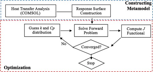
Figure 2 shows the workflow of the complete inverse problem methodology implemented. First, the response surface was constructed using values obtained from COMSOL. The constructed surrogate model was then coupled with the optimizer to minimize the J functional. The minimization of Equation (11) was performed using a hybrid of particle swarm and Broyden–Fletcher–Goldfarb–Shanno (BFGS) single-objective optimization algorithms [16,18]. The BFGS algorithm logic can be described as follows. Given an initial vector of the design variables, x_0, (parameters such as A and B) the corresponding initial value of the objective function, f (which in our case is the functional, J) and an approximate initial Hessian matrix B₀, the BFGS algorithm progresses as follows:

Figure 2. Flow chart of the inverse problem methodology.

Table

(1)	Evaluate the search direction pk by solving $B_k{\mathit{p}}_k=-\mathrm{\nabla }f\left({\mathit{x}}_k\right)$
(2)	Update ${\mathit{x}}_{k+1}={\mathit{x}}_k+{\alpha }_k{\mathit{p}}_k$ where ${\alpha }_k$ is an acceptable step size found using line search
(3)	Set ${\mathit{s}}_k={\alpha }_k{\mathit{p}}_k$
(4)	${\mathit{y}}_k=\mathrm{\nabla }f\left({\mathit{x}}_{k+1}\right)-\mathrm{\nabla }f\left({\mathit{x}}_k\right)$
(5)	$B_{k+1}=B_k+{\displaystyle \frac{{\mathbf{\text{y}}}_k{\mathbf{\text{y}}}_k^{\text{T}}}{{\mathbf{\text{ y}}}_k^{\text{T}}{\mathbf{\text{s}}}_k}}-{\displaystyle \frac{B_k{\mathbf{\text{s}}}_k{\mathbf{\text{s}}}_k^{\text{T}}{B}_k}{{\mathbf{\text{s}}}_k^{\text{T}}{B}_k{\mathbf{\text{s}}}_k}}$

The J functional converged to its global minimum (theoretically, it should be zero) when the converged values of the parameters in the analytical models for thermal conductivity and specific heat create such values for calculated temperatures at the boundaries that are the same as the ‘measured’ values the boundaries at each of the mmax time steps.

It should be pointed out that use of classical gradient-based minimization search algorithms alone (such as Levenberg–Marquardt algorithm [16]) could be highly unreliable. These minimization algorithms are known to converge to the nearest feasible local minimum [19] instead of the global minimum, especially in the nonlinear inverse parameter identification problems where topology of the functional J in Equation (11) in the parameter space almost certainly has a number of local minima.

All computations were performed on a single thread of Intel Xeon CPU [email protected] GHz with 256GB of RAM. Each transient COMSOL solution of Equation (1) took approximately 15 s, where mmax = 11 time steps were used in each of the three cases. The same non-structured computational grid of approximately 30,000 triangular finite elements was used for each analysis. The response surface generation (including the time for 40–90 high fidelity finite element solutions) consumed 600–1300 s. The optimizer, when coupled with the response surface, took approximately 50–60 s for each case to minimize the functional J in Equation (11). Thus, total computing time spent on solving each of the three cases presented in this paper was between 650 and 1400 s.

4. Numerical results for arbitrary 2D geometry

The proposed inverse problem methodology was validated for several cases considering linear and nonlinear spatial distributions of material properties in an arbitrary 2D geometry (Table 1).

Table 1. Geometry definition of a multiply connected 2D solid object considered in this work.

	Equation	# Cells on boundary
Boundary 1	$r=r_0-A\cos \left(3\theta \right)$, where $r_0=1,A=0.2,0.0\le \theta \le 2\pi$	250
Boundary 2	${\left[{\displaystyle \frac{x-0.4}{0.2}}\right]}^2+{\left[{\displaystyle \frac{y-0.2}{0.2}}\right]}^2=1$	198
Boundary 3	${\left[{\displaystyle \frac{x-0.1}{0.4}}\right]}^2+{\left[{\displaystyle \frac{y+0.5}{0.3}}\right]}^2=1$	346
Boundary 4	${\left[{\displaystyle \frac{x+0.5}{0.1}}\right]}^4+{\left[{\displaystyle \frac{y-0.2}{0.3}}\right]}^4=1$	213

Table 2 shows the thermal boundary conditions applied to each of the four boundaries shown in Figure 3. The boundary conditions were kept the same for each of the three cases presented in this paper. All heat fluxes in this work were considered to be inwards and normal to the surface.

Figure 3. Multiply connected 2D solid object geometry defined using equations in Table 1.

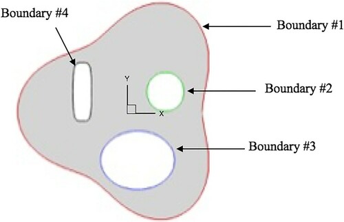
Table 2. Thermal boundary conditions applied to the multiply connected 2D geometry in Figure 3.

	Boundary conditions
Boundary #1	T = 353 K
Boundary #2	q = 100 k(x,y)
Boundary #3	q = 50 k(x,y)
Boundary #4	q = 125 k(x,y)

As previously stated, the distribution of thermal conductivity and specific heat was assumed to be defined according to some analytical prescribed functions. The assumed functions in this study were functions most commonly used to test optimization algorithms [20]. These functions are typically difficult to converge to as they are highly nonlinear, highly multimodal and feature several local minima.

4.1. Case 1: estimation of bilinear distribution of k(x,y) and C_p(x,y) in arbitrary 2D objects

Ability of this methodology was first tested assuming bilinear variations of thermal conductivity, Equation (12), and specific heat, Equation (13). In order to be consistent with units used, the right-hand side of Equation (12) should be multiplied with units of an arbitrary reference value of k(x,y) divided with units of length squared. For simplicity, the value of the reference thermal conductivity can be taken as one. Similar procedure should be followed with the right-hand side of Equation (13) when dealing with units. This means that the optimizer needs to find values of four parameters ($A_k,B_k,A_{C_p},B_{C_p}$) that minimize the J functional in Equation (11): (12) $k(x,y)=\left(A_k+x\right)\left(B_k+y\right)$(12) (13) $C_p(x,y)=\left(A_{C_p}+x\right)\left(B_{C_p}+y\right)$(13) The minimization algorithm was initialized with the particle swarm algorithm. A total of 100 swarm member were used where each swarm member was randomly initialized to lie within the bounds. Table 3 shows that the domain of search is relatively large, showing that the minimization technique can efficiently converge even with large allowable search region. If the analytical values fall outside of the bounds, the minimization algorithm will converge to the best possible values within those specified bounds.

Table 3. Case 1: search ranges for each of the four parameters, exact and converged values of the parameters defining thermal conductivity and specific heat.

	$A_k$	$B_k$	$A_{C_p}$	$B_{C_p}$
Min	0.0	0.0	0.0	0.0
Max	20.0	20.0	2.0	2.0
Exact	0.6	1.5	0.04	0.06
Estimated	0.6	1.5	0.04	0.06

Note: Functional J converged to value of less than 10⁻⁴.

The response surface for this test case was constructed [16] using 40 COMSOL analyses solutions of Equation (1). In reference [20], where the same analysis code was used, the relative error was approximately 0.012%, thus, certifying that COMSOL analysis with UDF option provides highly accurate solutions. Each of the solutions was obtained with different values of the four parameters. The response surface was then coupled with the modeFRONTIER optimizer [18]. Table 3 shows the exact values of the four parameters and the converged values of the parameters that define the thermal conductivity and specific heat distributions in Case 1. It is evident from Table 3 and Figure 4 that the optimizer was able to converge to the exact values of the four parameters, thereby accurately determining the spatial variations of the two material properties.

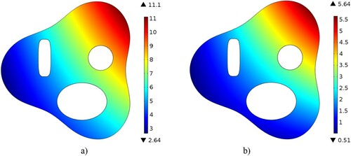
Figure 4. Case 1: distribution of (a) thermal conductivity and (b) specific heat.

4.2. Case 2: estimation of nonlinear distribution of k(x,y) and C_p (x,y) in arbitrary 2D objects

The proposed methodology was then tested for highly nonlinear spatial distributions of material properties. Thermal conductivity and specific heat were defined by the Matyas [20] function, Equation (14), and the McCormick [20] function, Equation (15), respectively: (14) $k(x,y)=A_k\left(x^2+y^2\right)-B_{k}xy$(14) (15) $C_p(x,y)=\text{sin}\left(A_{C_p}\left(x+y\right)\right)+B_{C_p}(x-y{)}^2-C_{C_p}x+D_{C_p}y+1$(15) Thus, the total of six parameters ($A_k,B_k,A_{C_p},B_{C_p},C_{C_p},D_{C_p}$) needed to be identified in Case 2 that minimize the J functional.

The response surface for this test case was constructed using 60 COMSOL analyses solutions, each analysis performed with different values of the six parameters. That is, the unsteady heat conduction equation was numerically integrated 60 times, each time with different random guesses for the six parameters that were determined using a quasi-random sequence generation algorithm of Sobol [17]. Using these 60 calculated values of the J functional, a six-dimensional response surface was generated using a radial basis function formulation.

Table 4 shows the exact and the optimizer converged values of the six parameters. It can be seen that even for a nonlinear spatial distribution of thermal conductivity and specific heat, this inverse parameter identification methodology was able to converge to the exact values of the six parameters.

Table 4. Case 2: search ranges for each of the six parameters, exact and converged values of the parameters defining thermal conductivity and specific heat.

	$A_k$	$B_k$	$A_{C_p}$	$B_{C_p}$	$C_{C_p}$	$D_{C_p}$
Min	0.0	−50.0	0.0	0.0	−2.0	0.0
Max	20.0	−10.0	2.0	2.0	0.0	2.0
Exact	13.6	−43.2	0.3	0.112	−0.012	0.021
Estimated	13.6	−43.2	0.3	0.112	−0.012	0.021

Note: Functional J converged to value of less than 10⁻⁴.

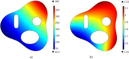
Figure 5 shows the nonlinear distribution of thermal conductivity and specific heat in Case 2.

Figure 5. Case 2: distribution of calculated: (a) thermal conductivity and (b) specific heat.

4.3. Case 3: estimation of nonlinear distribution of k(x,y) and C_p(x,y) with noisy measurements

In the previous sections, the inverse parameter identification methodology was validated for the linear and nonlinear spatial distribution of material properties. The ‘measured’ data, in the previous cases, was synthesized using COMSOL software. This does not accurately represent the real-life phenomenon. The ‘measured’ data are usually obtained through experimentation and therefore contain a certain level of noise. To accurately model such stochastic behaviour, noise must be added to the synthetic ‘measured’ data obtained using COMSOL. This was performed by employing the white Gaussian noise model to add noise [21], of varying intensity, to the ‘measured’ data.

In Case 3, the distribution of thermal conductivity was assumed to follow the generalized Three-Hump Camel Function [20], Equation (16), while specific heat was again assumed to follow the generalized McCormick function [20], Equation (15): (16) $k(x,y)=A_k{x}^2-B_k{x}^4+C_k{x}^6+D_{k}xy+E_k{y}^2$(16) Therefore, the optimizer needed to find values of the nine parameters that minimize the J functional. The ‘measured’ boundary temperature values were stochastically perturbed (with zero mean) by a noise-to-signal ratio of 1%, 2% and 3%. In reality, the actual Type J, K, E, and T thermocouples and resistance temperature detectors (RTDs) all have a maximum error of approximately 1% [22].

The nine-dimensional response surface was generated using 90 COMSOL analyses solutions corresponding to 90 sets of the nine parameters the values of which were determined using Sobol’s algorithm [17]. Because the objective function space in Case 3 was highly nonlinear due to the noisy ‘measurements’, a more robust hybrid optimizer [23,24] with an automatic switching logic among constituent single-objective optimization algorithms was needed to minimize J functional reliably.

Table 5 shows the exact values and converged calculated values of the nine parameters for various levels of measurement errors. It can be seen that when the measurement noise increases, the optimizer is still able to converge to correct parameters.

Table 5. Case 3: search ranges for each of the nine parameters, exact and converged values of the parameters defining thermal conductivity and specific heat for various specified noise levels in the ‘measurements' of boundary temperatures.

Min	Ak	Bk	Ck	Dk	Ek	Acp	Bcp	Ccp	Dcp
Min	0.0	−5.0	0.0	0.0	0.0	0.0	0.0	−2.0	0.0
Max	20.0	0.0	5.0	20.0	20.0	2.0	2.0	0.0	2.0
Exact	2.0	−1.05	0.1667	1.00	1.00	0.30	0.112	−0.012	0.021
Estimated (0% error)	2.0	−1.05	0.1667	1.00	1.00	0.30	0.112	−0.012	0.021
Estimated (1% error)	2.0	−1.04	0.1668	0.99	0.99	0.30	0.112	−0.012	0.021
Estimated (2% error)	2.0	−1.04	0.1668	1.00	1.00	0.30	0.112	−0.012	0.021
Estimated (3% error)	2.0	−1.03	0.175	0.93	1.01	0.30	0.109	−0.030	0.027

Note: Functional J converged to value of less than 10⁻⁴.

Figures 6 and 7 show the distribution of thermal conductivity and specific heat respectively in Case 3. It can be seen that even for higher values of boundary temperature measurement noise levels, both material properties were predicted accurately using this inverse parameter estimation methodology.

Figure 6. Case 3: spatial distribution of thermal conductivity obtained when boundary temperature measurement noise levels were (a) 0%, (b) 1%, (c) 2%, and (d) 3%.

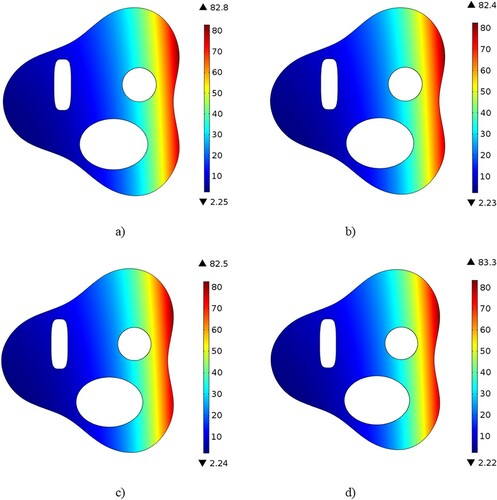
Figure 7. Case 3: spatial distribution of specific heat obtained when boundary temperature measurement noise levels were (a) 0%, 1%, 2% and (b) 3%.

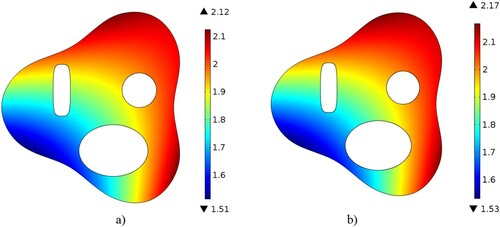
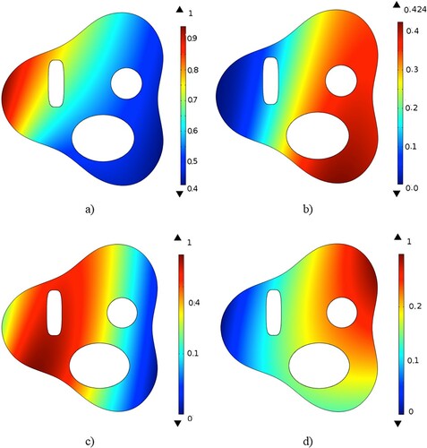
Figure 8 shows the relative error distributions for thermal conductivity and specific heat between their exact and converged values. It can be seen that the maximum local relative error is less than 1% even for large errors in the ‘measured’ boundary values of temperature, confirming that this inverse parameter identification method is robust and accurate.

Figure 8. Case 3: spatial distribution of relative error in percent between exact thermal conductivity and converged conductivity with (a) 1% noise, (b) 2% noise, and (c) 3% noise and (d) relative error between exact specific heat and converged specific heat with 3% measurement noise.

It should be pointed out that the key factors contributing to this successful methodology are the use of a highly robust and accurate hybrid single-objective optimization algorithm [23,24], use of a highly accurate multi-dimensional response surface [16], and the fact that we used a priori assumed general analytical spatial variations of thermal conductivity and specific heat.

5. Effects of measurement points on convergence

In the previous three sections, it was assumed that the temperature measurements are available at every boundary node. This is only true when using an infrared thermography or other thermal imaging techniques, but not always true when using sensors or thermocouples. If only point-measurement apparatus is available, then the effects on the number of temperature measurements on the convergence of the inverse problem solution method should be investigated. For this purpose, thermal conductivity, heat capacity and boundary conditions were assumed to follow the distribution defined in Case 3. A ‘measurement error’ with a noise-to-signal ratio of 3% was added to the boundary values (Table 2). The measurement points were randomly distributed on the boundaries of the geometry.

Figure 9 shows the effect of the number of boundary measurement points on the convergence of the material coefficients. It can be seen from Figure 9(a) and (b) that the relative error in the calculated coefficients is relatively low when using at least 40% of all boundary measurements. The general trend in Figure 9(a) and (b) indicates that a larger number of measurements results in better convergence. Figure 9(c) shows how the analytical and converged J functional (Equation (11)) varies with the number of measurements.

Figure 9. Effects of number of measurement points on (a) coefficients of thermal conductivity, (b) coefficient of heat capacity, and (c) the J functional.

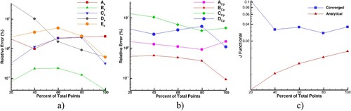
Here, the analytical value of J functional was obtained by solving Equation (1), while the converged value of the J functional was obtained from the response surface. It can be seen that by increasing the number of measuring points results in a higher J functional. This is because of the additional noise/error that is introduced by each additional sensor/thermocouple.

6. Conclusions

The methodology for estimating parameters in analytic models for the spatial distribution of thermal conductivity was extended to also estimate parameters in analytic models for the spatial distribution of specific heat within arbitrarily shaped multiply connected 2D solid objects. The material property can be non-destructively estimated by minimizing the sum of properly normalized squared differences between the calculated and measured boundary temperature on the surfaces of the object. The numerical integration of the governing parabolic partial differential equation for unsteady temperature evolution was performed using the finite element method based COMSOL software with the UDF capability. Accuracy of the steady-state temperature field was validated against an analytic solution.

An efficient surrogate model in the form of a multi-dimensional response surface supported by a relatively small number of the high fidelity finite element solutions was created to facilitate very fast approximate solutions of the analysis problem, thereby significantly reducing computing time for the minimization algorithm to converge. This inverse parameter identification method demonstrated promising results in being able to accurately and simultaneously determine linear and highly nonlinear spatial distributions of these two thermal properties. This method has also proven to be stable, thus, robust and accurate even when the boundary temperature measurements contained significant noise. Effects of the number of measurement points on convergence were also demonstrated.

The main requirements for the success of this inverse parameter estimation algorithm are the use of a highly reliable and accurate hybrid single-objective minimization algorithm and the use of as accurate as possible response surface generation algorithm.

Acknowledgement

The views and conclusions contained herein are those of the authors and should not be interpreted as necessarily representing the official policies or endorsements, either expressed or implied, of NSF, US Army or the US Government.

Disclosure statement

No potential conflict of interest was reported by the authors.

Additional information

Funding

The lead author gratefully acknowledges the financial support from Florida International University in the form of an FIU Presidential Fellowship and FIU Dissertation Year Fellowship. The authors are grateful for the research funding provided by the National Science Foundation research grant NSF CBET-1642253 monitored by Dr Jose Lage and for the HPC computing equipment provided by the U.S. Army under the equipment grant W911NF-16-1-0494.

References

- Chen WH, Seinfeld JH. Estimation of spatially varying parameters in partial differential equations. Int J Control. 1972;15:487–495. doi: https://doi.org/10.1080/00207177208932164
- Kitamura S, Nakagiri S. Identifiability of spatially-varying and constant parameters in distributed systems of parabolic type. SIAM J Control Optim. 1977;15:785–802. doi: https://doi.org/10.1137/0315050
- Goodson RE, Polis MP. Identification of parameters in distributed systems. In: WH Ray, DG Lainiotis, editors. Distributed parameter systems: identification, estimation, and control. New York (NY): Marcel Dekker; 1978. p. 47–133.
- Kravaris C, Seinfeld JH. Identification of parameters in distributed parameter systems by regularization. SIAM J Control Optim. 1985;23:217–241. doi: https://doi.org/10.1137/0323017
- Flach GP, Ozisik MN. Inverse heat conduction problem of simultaneously estimating spatially varying thermal conductivity and heat capacity per unit volume. Numer Heat Transf Part A: Appl. 1989;16(2):249–266. doi: https://doi.org/10.1080/10407788908944716
- Huang C-H, Ozisik MN. A direct integration approach for simultaneously estimating spatially varying thermal conductivity and heat capacity. Int J Heat Fluid Flow. 1990;11(3):262–268. doi: https://doi.org/10.1016/0142-727X(90)90047-F
- Rodrigues FA, Orlande HRB, Dulikravich GS. Simultaneous estimation of spatially-dependent diffusion coefficient and source term in nonlinear 1D diffusion problem. Math Comput Simul. 2004;66:409–424. doi: https://doi.org/10.1016/j.matcom.2004.02.005
- Huang C-H, Huang C-Y. An inverse problem in estimating simultaneously the effective thermal conductivity and volumetric heat capacity of biological tissue. Appl Math Modell. 2007;31:1785–1797. doi: https://doi.org/10.1016/j.apm.2006.06.002
- Naveira-Cotta C, Orlande HRB, Cotta R. Combining integral transforms and Bayesian inference in the simultaneous identification of variable thermal conductivity and thermal capacity in heterogeneous media. ASME J Heat Transf. 2011;133:111301–111311. doi: https://doi.org/10.1115/1.4004010
- Ozisik MN. Heat conduction. 2nd ed. New York (NY): Wiley; 1993. p. 571–616.
- Dulikravich GS, Reddy SR, Pasqualette MA, et al. Inverse determination of spatially varying material coefficients in solid objects. J Inverse Ill-Posed Probl. 2016;24(2):181–194. doi: https://doi.org/10.1515/jiip-2015-0057
- Reddy SR, Dulikravich GS, Zeidi SMJ. Non-destructive estimation of spatially varying thermal conductivity in 3D objects using boundary thermal measurements. Int J Therm Sci. 2017;118:488–496. doi: https://doi.org/10.1016/j.ijthermalsci.2017.05.011
- Pacheco CC, Vesenjak M, Borovinsek M, et al. Inverse parameter identification in solid mechanics using Bayesian statistics, response surfaces and minimization. Techn Mech. 2016;36(1–2):120–131.
- Reddy SR, Dulikravich GS, Zeidi SM. Inverse determination of spatially varying thermal capacity and thermal conductivity in arbitrary 2D objects. International Symposium on Advances in Computational Heat Transfer CHT-17; Naples, Italy, May 28–June 1; 2017.
- COMSOL Multiphyics V4.4, www.comsol.com
- Colaço MJ, Dulikravich GS. A survey of basic deterministic, heuristic and hybrid methods for single-objective optimization and response surface generation. In: Orlande HRB, Fudym O, Maillet D, et al., editors. Thermal measurements and inverse techniques. New York (NY): Taylor & Francis; 2011. p. 355–405.
- Sobol IM. On the distribution of points in a cube and the approximate evaluation of integrals. USSR Comput Math Math Phys. 1967;7:86–112. doi: https://doi.org/10.1016/0041-5553(67)90144-9
- modeFRONTIER, Software Package, Ver. 4.5.4, ESTECO, Trieste, Italy, 2014.
- Kanevce GH, Kanevce LP, Dulikravich GS. An inverse method for drying processes at high mass transfer Biot number. ASME Paper HT2003-40146, ASME Summer Heat Transfer Conference, Las Vegas, NV, July 21–23, 2003.
- Adorio EP. MVF – multivariate test functions library in C for unconstrained global optimization, 2005. http://geocities.com/eadorio/mvf.pdf.
- MATLAB and Statistics Toolbox Release 2012b, awgn function. The MathWorks, Inc., Natick, MA, USA, 2012.
- http://www.omega.com/Temperature/, visited 29 August 2016
- Dulikravich GS, Martin TJ, Dennis BH, et al. Multidisciplinary hybrid constrained GA optimization. In: K Miettinen, MM Makela, P Neittaanmaki, J Periaux, editors. EUROGEN99 – evolutionary algorithms in engineering and computer science: recent advances and industrial applications Jyvaskyla: John Wiley & Sons; 1999. p. 233–259.
- Dulikravich GS, Martin TJ, Colaco MJ, et al. Automatic switching algorithms in hybrid single-objective optimizers. FME Trans. 2013;41(3):167–179.