Fourier truncation method for the non-homogeneous time fractional backward heat conduction problem

Abstract

This paper is devoted to the problem of determining the initial data for the backward non-homogeneous time fractional heat conduction problem by the Fourier truncation method. The exact solution for the forward and backward fractional heat problems is expressed in terms of eigen function expansion and Mittag–Leffler function. Due to the instability of determining initial data, a regularized truncated solution is considered. Further, the stability estimate for the exact solution and the convergence estimates for the regularized solution using an á-priori choice rule and an á-posteriori choice rule are derived.

Keywords:

• Inverse problems
• ill-posed problems
• regularization
• truncation method
• heat equation
• fractional derivative
• Mittag–Leffler function

AMS CLASSIFICATIONS:

• 35R30
• 35K05
• 26A33
• 33E12

1. Introduction

Currently, a lot of research activities on the time fractional diffusion equations has been taking place due to its importance in several areas of science and engineering such as for describing the memory as well as hereditary properties for super diffusion and subdiffusion phenomena in the theory of plasma turbulence [1,2], random walks [3,4], viscoelastic material, biological systems [5] and in various other physical models [6]. Not only in physics and biological sciences, fractional heat equation has rich mathematical treatments on numerical simulation and regularity results (see, e.g. [7–13]). For heat conduction problems with time fractional partial derivative, one may be interested in the inverse problem determining boundary or initial data, or diffusion coefficients, or source term using certain measurements. Such problems are ill-posed, in the sense that small perturbations in the data can lead to large deviations in the solutions (see, e.g. [14,15]).

Throughout the paper, we take $\mathrm{\Omega }:=(0,\pi )$ and $I_{\tau }:=[0,\tau ]$ for some $\tau >0$. We consider the non-homogeneous time fractional heat equation (1) $u_t^{\alpha }(x,t)-u_{xx}(x,t)=f(x,t),(x,t)\in \mathrm{\Omega }\times (0,\tau ]$(1) along with the following conditions: (2) $u(0,t)=0,u(\pi ,t)=0,t\in I_{\tau },$(2) for $0<\alpha <1$. Here, $u_t^{\alpha }(x,t)$ is the α-order time fractional partial derivative of u with respect to t, that is, $u_t^{\alpha }(x,t)=\frac{1}{\mathrm{\Gamma }(1-\alpha )}{\int }_0^t\frac{u_s(x,s)}{(t-s{)}^{\alpha }}\mathrm{d}s,(x,t)\in \mathrm{\Omega }\times (0,\tau ].$ For a known source function $f(\cdot ,\cdot )$, the time fractional backward heat conduction problem (TFBHCP) that we consider is the following inverse problem.

Given $f\in L^{\mathrm{\infty }}(I_{\tau },L^2(\mathrm{\Omega }\left)\right)$ and $\eta \in L^2\left(\mathrm{\Omega }\right)$, find $u(x,t)$ satisfying (1(1) $u_t^{\alpha }(x,t)-u_{xx}(x,t)=f(x,t),(x,t)\in \mathrm{\Omega }\times (0,\tau ]$(1) ) and (2(2) $u(0,t)=0,u(\pi ,t)=0,t\in I_{\tau },$(2) ), and the final value requirement $u(x,\tau )=\eta \left(x\right),x\in \mathrm{\Omega }$.

Thus the problem is to solve Equation (1(1) $u_t^{\alpha }(x,t)-u_{xx}(x,t)=f(x,t),(x,t)\in \mathrm{\Omega }\times (0,\tau ]$(1) ) satisfying (2(2) $u(0,t)=0,u(\pi ,t)=0,t\in I_{\tau },$(2) ) and the requirement (3) $u(x,\tau )=\eta \left(x\right),x\in \mathrm{\Omega }.$(3) We shall see that the above problem of determining $u(x,t)$ for t>0 is well-posed, whereas determining $u(x,0)$ is ill-posed, in the sense that small perturbations in the data η can result in large deviation in the solution.

For a function $f:\mathrm{\Omega }\times I_{\tau }\to \mathbb{R}$ and $t\in [0,\tau ]$, by abusing the notation, we shall denote the function $x\mapsto f(x,t)$ from Ω to $\mathbb{R}$ by $f\left(t\right)$. Thus $f\left(t\right)\left(x\right):=f(x,t),(x,t)\in \mathrm{\Omega }\times I_{\tau }.$ Thus $f\in L^{\mathrm{\infty }}(I_{\tau },L^2(\mathrm{\Omega }\left)\right)$ if and only if the function $t\mapsto f\left(t\right)$ is an $L^2\left(\mathrm{\Omega }\right)$-valued measurable function such that $\underset{t\in I_{\tau }}{sup}\parallel f\left(t\right){\parallel }_{L^2\left(\mathrm{\Omega }\right)}<\mathrm{\infty }.$ It is known that $L^{\mathrm{\infty }}(I_{\tau },L^2(\mathrm{\Omega }\left)\right)$ is a Banach space with norm $\parallel f{\parallel }_{L^{\mathrm{\infty }}(I_{\tau },L^2(\mathrm{\Omega }\left)\right)}:=\underset{t\in I_{\tau }}{sup}\parallel f\left(t\right){\parallel }_{L^2\left(\mathrm{\Omega }\right)}.$ We are concerned with the problem of determining the initial temperature $u(\cdot ,0)$ from the measured final temperature $\tilde{\eta }\sim u(\cdot ,\tau )$ and the measured source term $\tilde{f}\sim f$ with some noise level $\delta >0$. As this problem is known to be ill-posed, some regularization method is required for obtaining stable approximations for a sought solution. For detailed study on regularization of partial differential equation and for regularization of linear ill-posed operator equations, one may refer Isakov [16] and Nair [17], respectively.

In the literature, we can find a few papers on recovering initial data for homogeneous TFBHCP, that is for f=0, by some regularization methods, such as quasi reversibility [18] in 2010, data regularization [19] and boundary condition regularization [20] in 2013, Tikhonov scheme [21] in 2013, modified quasi boundary value method [22] in 2014 and generalized Tikhonov scheme [23] in 2017. Very recently, Tuan et al. in [24] and [25] considered non-homogeneous TFBHCP of determining initial data from final data and source term by using a quasi boundary value method and Tikhonov method respectively.

It is clear that the research work related to the problem of determining initial data from final and source data for TFBHCP is still in the initial stage. Motivated by this fact, this work is devoted to the problem of determining the initial data for the non-homogeneous TFBHCP by the measured final data and the measured source term with some noise level, by using the standard easy-to-comprehend procedure of the Fourier Truncation method.

This paper is organized as follows: In Section 2, basic results from fractional calculus are stated. After that, the solution for the forward and backward time fractional heat conduction problems is derived. We also show that problem of determining $u(x,t)$ for t>0 is well-posed, whereas determining $u(x,0)$ is ill-posed, in the sense that small perturbations in the data η can result in large deviation in the solution. In Section 3, instability of initial data and its conditional stability under the priori bound are analysed. In Sections 4 and 5, a regularized solution is formulated by cutting off the high frequencies on Fourier coefficients and choosing the number of Fourier coefficients (regularization parameter) depending on the error level in the noisy data. Further, we obtain error estimates for the regularized solution by choosing the regularization parameter, namely the level of truncation, by an á-priori as well as an á-posteriori rules.

2. Preliminaries

2.1. Some basic results from fractional calculus

Let us recall the definition and some results associated with Riemann–Liouville fractional integral, Caputo fractional derivative and Mittag–Leffler function as given in [26,27].

In this paper, we shall be concerned only with left Riemann–Liouville fractional integral and left Caputo fractional derivative, and we denote them by $I^{\alpha }$ and $D^{\alpha }$, respectively, and we denote $\left(D^{\alpha }f\right)\left(t\right)$ by $f^{\alpha }\left(t\right)$. Thus $\begin{array}{rl}\left(I^{\alpha }f\right)\left(t\right)& :=\frac{1}{\mathrm{\Gamma }\left(\alpha \right)}{\int }_0^t(t-s{)}^{\alpha -1}f(s)\mathrm{d}s,t\in (0,\tau ],\\ f^{\alpha }\left(t\right)& :=D^{\alpha }f\left(t\right):=\frac{1}{\mathrm{\Gamma }(1-\alpha )}{\int }_0^t(t-s{)}^{-\alpha }{f}^{\mathrm{\prime }}(s)\mathrm{d}s,t\in (0,\tau ].\end{array}$ We may recall that Riemann–Liouville fractional integral and Caputo fractional derivative can be defined for any $\alpha >0$ and for $t\in [0,\mathrm{\infty })$ for appropriate functions (see [26]). However, we restrict these definitions to the case of $0<\alpha <1$ and $t\in [0,\tau ]$.

Recall also that (see [27]), for $\alpha >0$ and $\text{β}>0$, the Mittag–Leffler function $E_{\alpha ,\text{β}}$ is defined by $E_{\alpha ,\text{β}}\left(z\right):=\sum _{k=0}^{\mathrm{\infty }}\frac{z^k}{\mathrm{\Gamma }(\alpha k+\text{β})},z\in \mathbb{C}.$ We shall denote $E_{\alpha ,1}\left(z\right)$ by $E_{\alpha }\left(z\right)$, that is, $E_{\alpha }\left(z\right):=\sum _{k=0}^{\mathrm{\infty }}\frac{z^k}{\mathrm{\Gamma }(\alpha k+1)},z\in \mathbb{C}.$ We may observe that the above function is a generalization of the exponential function $e^z$, in the sense that $E_{1,1}\left(z\right)=e^z$. Further, we also have $E_{1,2}\left(z\right)=\frac{e^z-1}{z},E_{2,1}\left(z^2\right)=\cosh \left(z\right),E_{2,2}\left(z^2\right)=\frac{\sinh z}{z}.$ Associated with $E_{\alpha ,\text{β}}$, we quote a few results, which we shall use in the due course.

Lemma 2.1

(cf. [13], Lemma (3.2) and (3.3)) For $0<\alpha <1$ and $\mu >0$, the following are true.

1. The function $t\mapsto E_{\alpha }(-\mu t^{\alpha })$ is continuous on $I_{\tau }$ and for each $j\in \mathbb{N}$, $\frac{{\mathrm{d}}^j}{\mathrm{d}{t}^j}{E}_{\alpha }(-\mu t^{\alpha })=\sum _{n=0}^{\mathrm{\infty }}\frac{{\mathrm{d}}^j}{\mathrm{d}{t}^j}\frac{(-\mu t^{\alpha }{)}^n}{\mathrm{\Gamma }(\alpha n+1)}=-\mu t^{\alpha -j}{E}_{\alpha ,\alpha -j+1}(-\mu t^{\alpha }),t>0.$ In particular, $\frac{\mathrm{d}}{\mathrm{d}t}{E}_{\alpha }(-\mu t^{\alpha })=-\mu t^{\alpha -1}{E}_{\alpha ,\alpha }(-\mu t^{\alpha }),t>0.$

2. The function $t\mapsto t^{\alpha -1}{E}_{\alpha ,\alpha }(-\mu t^{\alpha })$ belongs to $L^1\left(I_{\tau }\right)$ and ${\int }_0^{\tau }|t^{\alpha -1}{E}_{\alpha ,\alpha }(-\mu t^{\alpha })|\mathrm{d}t\le \frac{1}{\mu }.$

Lemma 2.2

(cf. [18]) Let $0<{\alpha }_0<{\alpha }_1<1$. Then there exists positive constants $C_{+}$ and $C_{-}$, depending on ${\alpha }_0,{\alpha }_1$, such that (4) $\frac{C_{-}}{\mathrm{\Gamma }(1-\alpha )(1-x)}\le E_{\alpha }\left(x\right)\le \frac{C_{+}}{\mathrm{\Gamma }(1-\alpha )(1-x)},$(4) for all $x\le 0$ and for all $\alpha \in [{\alpha }_0,{\alpha }_1].$

Corollary 2.3

(cf. [21]) Let $0<{\alpha }_0<{\alpha }_1<1$ and ${\mu }_0>0$. Then there exist positive constants $C_1,C_2$, depending on ${\alpha }_0,{\alpha }_1,\tau ,{\mu }_0$ such that (5) $\frac{C_2}{\mu }\le E_{\alpha }(-\mu {\tau }^{\alpha })\le \frac{C_1}{\mu }$(5) for all $\mu \ge {\mu }_0$ and for all $\alpha \in [{\alpha }_0,{\alpha }_1]$.

2.2. Solution for the forward fractional heat conduction problem

For $f\in L^{\mathrm{\infty }}(I_{\tau },L^2(\mathrm{\Omega }\left)\right)$ and $\psi \in L^2\left(\mathrm{\Omega }\right)$, consider the non-homogeneous forward time fractional heat conduction problem, (6) $u_t^{\alpha }(x,t)-u_{xx}(x,t)=f(x,t),x,t)\in \mathrm{\Omega }\times (0,\tau ]$(6) along with the boundary conditions (7) $u(0,t)=0,u(\pi ,t)=0,t\in [0,\tau ],$(7) and the initial condition (8) $u(x,0)=\psi \left(x\right),x\in \mathrm{\Omega }.$(8) It can be shown that $u_t^{\alpha }\to u_t$ as $\alpha \to 1$. Hence, in the limiting case, the heat equation (6(6) $u_t^{\alpha }(x,t)-u_{xx}(x,t)=f(x,t),x,t)\in \mathrm{\Omega }\times (0,\tau ]$(6) ) is reduced to the standard heat equation. We shall also see that ( see Theorem 2.6) if $u_{\alpha }(\cdot ,\cdot )$ is a solution of (6(6) $u_t^{\alpha }(x,t)-u_{xx}(x,t)=f(x,t),x,t)\in \mathrm{\Omega }\times (0,\tau ]$(6) ), (7(7) $u(0,t)=0,u(\pi ,t)=0,t\in [0,\tau ],$(7) ), (8(8) $u(x,0)=\psi \left(x\right),x\in \mathrm{\Omega }.$(8) ), and if ${\displaystyle u(x,t)=\underset{\alpha \to 1}{lim}{u}_{\alpha }(x,t)}$ for $(x,t)\in \mathrm{\Omega }\times (0,\tau ]$, then $u(\cdot ,\cdot )$ satisfies the standard heat equation (9) $u_t(x,t)-u_{xx}(x,t)=f(x,t),(x,t)\in \mathrm{\Omega }\times (0,\tau ]$(9) along with the conditions in (7(7) $u(0,t)=0,u(\pi ,t)=0,t\in [0,\tau ],$(7) ) and (8(8) $u(x,0)=\psi \left(x\right),x\in \mathrm{\Omega }.$(8) ).

With the help of the following lemmas, we shall represent the solution of the forward fractional heat conduction problem (6(6) $u_t^{\alpha }(x,t)-u_{xx}(x,t)=f(x,t),x,t)\in \mathrm{\Omega }\times (0,\tau ]$(6) )–(8(8) $u(x,0)=\psi \left(x\right),x\in \mathrm{\Omega }.$(8) ).

Throughout the paper, we use the notation ${\lambda }_n:=n^2\text{and}{\varphi }_n\left(x\right):=\sqrt{\frac{2}{\pi }}\sin \left(nx\right)$ for $x\in \mathrm{\Omega }$ and $n\in \mathbb{N}$. Note that $\{{\varphi }_k:k\in \mathbb{N}\}$ is an orthonormal basis of $L^2\left(\mathrm{\Omega }\right)$. Also, for $g\in L^2[0,\pi ]$, we denote the $L^2$-inner product of g with ${\varphi }_k$, namely, $⟨g,{\varphi }_k⟩$ by $g_k$, that is, $g_k:=⟨g,{\varphi }_k⟩,k\in \mathbb{N}$ and for a function $f:I_{\tau }\to L^2\left(\mathrm{\Omega }\right)$ and $s\in I_{\tau }$, we denote $⟨f\left(s\right),{\varphi }_k⟩$ by $f_k\left(s\right)$, that is, $f_k\left(s\right):=⟨f\left(s\right),{\varphi }_k⟩,k\in \mathbb{N}.$ For $g\in L^2\left(\mathrm{\Omega }\right)$ and $h\in L^{\mathrm{\infty }}(I_{\tau },L^2(\mathrm{\Omega }\left)\right)$, we shall denote $\parallel g\parallel :=\parallel g{\parallel }_{L^2\left(\mathrm{\Omega }\right)},\parallel h{\parallel }_{\mathrm{\infty }}:=\parallel h{\parallel }_{L^{\mathrm{\infty }}(I_{\tau },L^2(\mathrm{\Omega }\left)\right)}.$

Lemma 2.4

(cf. [28], Lemma 2.9) For $0<\alpha <1,\mu >0,q\in L^{\mathrm{\infty }}\left(I_{\tau }\right)$, and ${\phi }_0\in \mathbb{R}$, the function $\phi \in C\left(I_{\tau }\right)$ defined by (10) $\phi \left(t\right)=E_{\alpha }(-\mu t^{\alpha }){\phi }_0+{\int }_0^t(t-s{)}^{\alpha -1}{E}_{\alpha ,\alpha }(-\mu (t-s{)}^{\alpha })q\left(s\right)\mathrm{d}s$(10) satisfies the fractional initial value problem (11) $\begin{array}{rl}\frac{{\mathrm{d}}^{\alpha }\phi }{\mathrm{d}{t}^{\alpha }}+\mu \phi \left(t\right)& =q\left(t\right),t\in (0,\tau ]\\ \phi \left(0\right)& ={\phi }_0.\end{array}$(11) The following result on forward fractional heat conduction problem (6(6) $u_t^{\alpha }(x,t)-u_{xx}(x,t)=f(x,t),x,t)\in \mathrm{\Omega }\times (0,\tau ]$(6) )–(8(8) $u(x,0)=\psi \left(x\right),x\in \mathrm{\Omega }.$(8) ) is well known [12].

Theorem 2.5

Let $0<\alpha <1$. For $\psi \in L^2\left(\mathrm{\Omega }\right)$ and $f\in L^{\mathrm{\infty }}(I_{\tau };L^2(\mathrm{\Omega }\left)\right)$, the function $u_{\alpha }(\cdot ,\cdot )$ defined by (12) $u_{\alpha }(x,t)=\sum _{k=1}^{\mathrm{\infty }}\left[E_{\alpha }(-{\lambda }_k{t}^{\alpha }){\psi }_k+{\int }_0^t(t-s{)}^{\alpha -1}{E}_{\alpha ,\alpha }(-{\lambda }_k(t-s{)}^{\alpha })f_k\left(s\right)\mathrm{d}s\right]{\varphi }_k\left(x\right)$(12) is the solution of the forward fractional heat conduction problem (6(6) $u_t^{\alpha }(x,t)-u_{xx}(x,t)=f(x,t),x,t)\in \mathrm{\Omega }\times (0,\tau ]$(6) )–(8(8) $u(x,0)=\psi \left(x\right),x\in \mathrm{\Omega }.$(8) ).

Hereafter, for $0<\alpha <1$ and $f:I_{\tau }\to L^2\left(\mathrm{\Omega }\right)$, $t\in I_{\tau }$, and $k\in \mathbb{N}$, we shall also use the notation (13) $F_{\alpha ,k}\left(t\right):={\int }_0^t(t-s{)}^{\alpha -1}{E}_{\alpha ,\alpha }(-{\lambda }_k(t-s{)}^{\alpha })f_k\left(s\right)\mathrm{d}s.$(13) The next theorem shows how the solution of the standard heat equation (9(9) $u_t(x,t)-u_{xx}(x,t)=f(x,t),(x,t)\in \mathrm{\Omega }\times (0,\tau ]$(9) ) along with the boundary condition (7(7) $u(0,t)=0,u(\pi ,t)=0,t\in [0,\tau ],$(7) ) and the initial condition (8(8) $u(x,0)=\psi \left(x\right),x\in \mathrm{\Omega }.$(8) ) is the limit of $u_{\alpha }(x,t)$ as $\alpha \to 1$. This result is known and is stated in the literature. As the form of the solution is used throughout the paper, we include its proof also.

Theorem 2.6

For $0<\alpha <1$, let $u_{\alpha }(x,t)$ be the solution of the forward fractional heat conduction problem (6(6) $u_t^{\alpha }(x,t)-u_{xx}(x,t)=f(x,t),x,t)\in \mathrm{\Omega }\times (0,\tau ]$(6) )–(8(8) $u(x,0)=\psi \left(x\right),x\in \mathrm{\Omega }.$(8) ), $u_{\alpha }(x,t)=\sum _{k=1}^{\mathrm{\infty }}\left[E_{\alpha }(-{\lambda }_k{t}^{\alpha }){\psi }_k+F_{\alpha ,k}\left(t\right)x\mathrm{d}s\right]{\varphi }_k\left(x\right),$ where $F_{\alpha ,k}$ is as in (13(13) $F_{\alpha ,k}\left(t\right):={\int }_0^t(t-s{)}^{\alpha -1}{E}_{\alpha ,\alpha }(-{\lambda }_k(t-s{)}^{\alpha })f_k\left(s\right)\mathrm{d}s.$(13) ). Then ${\displaystyle \underset{\alpha \to 1}{lim}{u}_{\alpha }(x,t)}$ exists, and it is the solution of the standard heat equation (9(9) $u_t(x,t)-u_{xx}(x,t)=f(x,t),(x,t)\in \mathrm{\Omega }\times (0,\tau ]$(9) ) along with the boundary condition (7(7) $u(0,t)=0,u(\pi ,t)=0,t\in [0,\tau ],$(7) ) and the initial condition by (8).

Proof.

Let $0<\alpha <1$. For $n\in \mathbb{N}$, let $u_{\alpha ,n}(x,t):=\sum _{k=1}^n\left[E_{\alpha }(-{\lambda }_k{t}^{\alpha }){\psi }_k+F_{\alpha ,k}\left(t\right)\right]{\varphi }_k\left(x\right),$ where $F_{\alpha ,k}$ is as in (13(13) $F_{\alpha ,k}\left(t\right):={\int }_0^t(t-s{)}^{\alpha -1}{E}_{\alpha ,\alpha }(-{\lambda }_k(t-s{)}^{\alpha })f_k\left(s\right)\mathrm{d}s.$(13) ). Recall from Corollary 2.3 and Lemma 2.1 (ii) that $|E_{\alpha }(-\mu t^{\alpha })|\le \frac{C}{\mu }\text{and}{\int }_0^t|t^{\alpha -1}{E}_{\alpha ,\alpha }(-\mu t^{\alpha })|\mathrm{d}t\le \frac{1}{\mu }$ for any $\mu >0$. Also, $|{\psi }_k|\le \parallel \psi \parallel ,|{\varphi }_k\left(x\right)|\le \sqrt{\frac{2}{\pi }}$ and $|f_k\left(s\right)|\le \parallel f\left(s\right){\parallel }_{L^2\left(\mathrm{\Omega }\right)}\le \parallel f{\parallel }_{\mathrm{\infty }}:=\parallel f{\parallel }_{L^{\mathrm{\infty }}(I_{\tau },L^2(\mathrm{\Omega }\left)\right)}.$ Thus, for $k\in \mathbb{N}$, using Lemma (2.1) (ii), we have (14) $|F_{\alpha ,k}\left(t\right)|\le {\int }_0^t(t-s{)}^{\alpha -1}{E}_{\alpha ,\alpha }(-{\lambda }_k(t-s{)}^{\alpha })|f_k\left(s\right)|\mathrm{d}s\le \frac{1}{{\lambda }_k}\parallel f{\parallel }_{\mathrm{\infty }}$(14) and hence $|\left[E_{\alpha }\right(-{\lambda }_k{t}^{\alpha }){\psi }_k+F_{\alpha ,k}(t\left)\right]{\varphi }_k\left(x\right)|\le \frac{1}{{\lambda }_k}\sqrt{\frac{2}{\pi }}(C\parallel \psi \parallel +\parallel f{\parallel }_{\mathrm{\infty }}).$ Since $\sum _{k=1}^{\mathrm{\infty }}\frac{1}{{\lambda }_k}$ converges, it then follows that $u_{\alpha ,n}(x,t)\to u_{\alpha }(x,t)$ uniformly $n\to \mathrm{\infty }$.

On the other hand, using the facts that $\underset{\alpha \to 1}{lim}{E}_{\alpha }(-{\lambda }_k{t}^{\alpha })=e^{-{\lambda }_{k}t}\text{and}\underset{\alpha \to 1}{lim}{t}^{\alpha -1}{E}_{\alpha ,\alpha }(-{\lambda }_k{t}^{\alpha })=e^{-{\lambda }_{k}t}$ for all $k\in \mathbb{N}$, we have $\underset{\alpha \to 1}{lim}\left[E_{\alpha }(-{\lambda }_k{t}^{\alpha }){\psi }_k+F_{\alpha ,k}\left(t\right)\right]{\varphi }_k\left(x\right)=\left[e^{-{\lambda }_{k}t}{\psi }_k+{\int }_0^t{e}^{-{\lambda }_k(t-s)}{f}_k\left(s\right)\mathrm{d}s\right]{\varphi }_k\left(x\right).$ Thus for each $(x,t)\in \mathrm{\Omega }\times I_{\tau }$, $u_{\alpha ,n}(x,t)\to u_{\alpha }(x,t)$ uniformly for $\alpha \in (0,1]$ as $n\to \mathrm{\infty }$, and $\underset{\alpha \to 1}{lim}{u}_{\alpha ,n}(x,t)=u_{1,n}(x,t):=\sum _{k=1}^n\left[e^{-{\lambda }_{k}t}{\psi }_k+{\int }_0^t{e}^{-{\lambda }_k(t-s)}{f}_k\left(s\right)\mathrm{d}s\right]{\varphi }_k\left(x\right)$ for every $n\in \mathbb{N}$.

Hence, by a standard theorem in analysis (see Theorem 7.11 in Rudin [29]), $\underset{\alpha \to 1}{lim}{u}_{\alpha }(x,t)=\underset{n\to \mathrm{\infty }}{lim}\underset{\alpha \to 1}{lim}{u}_{\alpha ,n}(x,t).$ Note that $\underset{n\to \mathrm{\infty }}{lim}\underset{\alpha \to 1}{lim}{u}_{\alpha ,n}(x,t)=\sum _{k=1}^{\mathrm{\infty }}\left[e^{-{\lambda }_{k}t}{\psi }_k+{\int }_0^t{e}^{-{\lambda }_k(t-s)}{f}_k\left(s\right)\mathrm{d}s\right]{\varphi }_k\left(x\right)$ and it is the solution of the standard heat equation (9(9) $u_t(x,t)-u_{xx}(x,t)=f(x,t),(x,t)\in \mathrm{\Omega }\times (0,\tau ]$(9) ) along with the boundary condition (7(7) $u(0,t)=0,u(\pi ,t)=0,t\in [0,\tau ],$(7) ) and the initial condition (8(8) $u(x,0)=\psi \left(x\right),x\in \mathrm{\Omega }.$(8) ).

3. Existence of solution for TFBHCP

The following theorem, proved in [24], gives conditions on the functions η and f in (3(3) $u(x,\tau )=\eta \left(x\right),x\in \mathrm{\Omega }.$(3) ) and (1(1) $u_t^{\alpha }(x,t)-u_{xx}(x,t)=f(x,t),(x,t)\in \mathrm{\Omega }\times (0,\tau ]$(1) ), respectively, so that the TFBHCP (1(1) $u_t^{\alpha }(x,t)-u_{xx}(x,t)=f(x,t),(x,t)\in \mathrm{\Omega }\times (0,\tau ]$(1) )–(3(3) $u(x,\tau )=\eta \left(x\right),x\in \mathrm{\Omega }.$(3) ) with $0<\alpha <1$ has a unique solution.

Theorem 3.1

For $\eta \in L^2\left(\mathrm{\Omega }\right)$ and $f\in L^{\mathrm{\infty }}(I_{\tau };L^2(\mathrm{\Omega }\left)\right)$, the TFBHCP (1(1) $u_t^{\alpha }(x,t)-u_{xx}(x,t)=f(x,t),(x,t)\in \mathrm{\Omega }\times (0,\tau ]$(1) )–(3(3) $u(x,\tau )=\eta \left(x\right),x\in \mathrm{\Omega }.$(3) ) has a unique solution if and only if (15) $\sum _{k=1}^{\mathrm{\infty }}{\left(\frac{{\eta }_k-F_{\alpha ,k}\left(\tau \right)}{E_{\alpha }(-{\lambda }_k{\tau }^{\alpha })}\right)}^2<\mathrm{\infty },$(15) and it is given by (16) $u_{\alpha }(x,t)=\sum _{k=1}^{\mathrm{\infty }}\left[\frac{E_{\alpha }(-{\lambda }_k{t}^{\alpha })}{E_{\alpha }(-{\lambda }_k{\tau }^{\alpha })}\left[{\eta }_k-F_{\alpha ,k}\left(\tau \right)\right]+F_{\alpha ,k}\left(t\right)\right]{\varphi }_k\left(x\right)$(16) for $x\in \mathrm{\Omega }$ and $0\le t\le \tau$.

3.1. Solution under noisy data

Let us denote by $u_{\alpha }(x,t;\eta ,f)$ the solution $u_{\alpha }(x,t)$ defined as in (16(16) $u_{\alpha }(x,t)=\sum _{k=1}^{\mathrm{\infty }}\left[\frac{E_{\alpha }(-{\lambda }_k{t}^{\alpha })}{E_{\alpha }(-{\lambda }_k{\tau }^{\alpha })}\left[{\eta }_k-F_{\alpha ,k}\left(\tau \right)\right]+F_{\alpha ,k}\left(t\right)\right]{\varphi }_k\left(x\right)$(16) ) corresponding to the data $(\eta ,f)\in L^2\left(\mathrm{\Omega }\right)\times L^{\mathrm{\infty }}(I_{\tau };L^2(\mathrm{\Omega }\left)\right)$. Then the following theorem shows that $u_{\alpha }(x,t,\eta ,f)$ depends continuously on the data $(\eta ,f)$ whenever $0<t<\tau$.

Theorem 3.2

Let $\eta ,\tilde{\eta }\in L^2\left(\mathrm{\Omega }\right)$ and $f,\tilde{f}\in L^{\mathrm{\infty }}(I_{\tau },L^2(\mathrm{\Omega }\left)\right)$. Then, for $t\in (0,\tau )$, $\parallel u_{\alpha }(\cdot ,t;\eta ,f)-u_{\alpha }(\cdot ,t;\tilde{\eta },\tilde{f}){\parallel }^2\le 3C_{\alpha ,t}\parallel \eta -\tilde{\eta }{\parallel }^2+3{\zeta }_0(C_{t,\alpha }+1)\parallel f-\tilde{f}{\parallel }_{\mathrm{\infty }}^2,$ where $C_{\alpha ,t}:=\left(C_{+}/C_{-}{)}^2\right(\left(1+{\tau }^{\alpha }\right)/t^{\alpha }{)}^2$ and ${\zeta }_0:=\sum _{n=1}^{\mathrm{\infty }}1/n^4$.

Proof.

Let $t\in (0,\tau )$ and let ${\tilde{F}}_{\alpha ,k}$ be as in (13(13) $F_{\alpha ,k}\left(t\right):={\int }_0^t(t-s{)}^{\alpha -1}{E}_{\alpha ,\alpha }(-{\lambda }_k(t-s{)}^{\alpha })f_k\left(s\right)\mathrm{d}s.$(13) ) with f replaced by $\tilde{f}$. Then $\begin{array}{rl}{u}_{\alpha }(x,t;\eta ,f)& =\sum _{k=1}^{\mathrm{\infty }}\left[\frac{E_{\alpha }(-{\lambda }_k{t}^{\alpha })}{E_{\alpha }(-{\lambda }_k{\tau }^{\alpha })}\left[{\eta }_k-F_{\alpha ,k}\left(\tau \right)\right]+F_{\alpha ,k}\left(t\right)\right]{\varphi }_k\left(x\right)\\ u_{\alpha }(x,t;\tilde{\eta },\tilde{f})& =\sum _{k=1}^{\mathrm{\infty }}\left[\frac{E_{\alpha }(-{\lambda }_k{t}^{\alpha })}{E_{\alpha }(-{\lambda }_k{\tau }^{\alpha })}\left[{\tilde{\eta }}_k-{\tilde{F}}_{\alpha ,k}\left(\tau \right)\right]+{\tilde{F}}_{\alpha ,k}\left(t\right)\right]{\varphi }_k\left(x\right)\end{array}$ for $x\in \mathrm{\Omega }$ so that $\parallel u_{\alpha }(\cdot ,t;\eta ,f)-u_{\alpha }(\cdot ,t;\tilde{\eta },\tilde{f}){\parallel }^2=\sum _{k=1}^{\mathrm{\infty }}|{\text{β}}_{\alpha ,k}\left(t\right){|}^2,$ where ${\text{β}}_{\alpha ,k}\left(t\right):=\frac{E_{\alpha }(-{\lambda }_k{t}^{\alpha })}{E_{\alpha }(-{\lambda }_k{\tau }^{\alpha })}\left[({\eta }_k-{\tilde{\eta }}_k)-\left(F_{\alpha ,k}\right(\tau )-{\tilde{F}}_{\alpha ,k}(\tau \left)\right)\right]+\left(F_{\alpha ,k}\right(t)-{\tilde{F}}_{\alpha ,k}(t\left)\right).$ By Lemma 2.2, we have (17) $\frac{1}{C}\frac{(1+{\lambda }_k{\tau }^{\alpha })}{(1+{\lambda }_k{t}^{\alpha })}\le \frac{E_{\alpha }(-{\lambda }_k{t}^{\alpha })}{E_{\alpha }(-{\lambda }_k{\tau }^{\alpha })}\le C\frac{(1+{\lambda }_k{\tau }^{\alpha })}{(1+{\lambda }_k{t}^{\alpha })}\le C\frac{1+{\tau }^{\alpha }}{t^{\alpha }},$(17) where $C:=C_{+}/C_{-}.$ Therefore, $\begin{array}{rl}|{\text{β}}_{\alpha ,k}\left(t\right)|& \le |\frac{E_{\alpha }(-{\lambda }_k{t}^{\alpha })}{E_{\alpha }(-{\lambda }_k{\tau }^{\alpha })}|(|{\eta }_k-{\tilde{\eta }}_k|+|F_{\alpha ,k}\left(\tau \right)-{\tilde{F}}_{\alpha ,k}\left(\tau \right)|)+|F_{\alpha ,k}\left(t\right)-{\tilde{F}}_{\alpha ,k}\left(t\right))|\\ & \le C\left(\frac{1+{\tau }^{\alpha }}{t^{\alpha }}\right)\left(|{\eta }_k-{\tilde{\eta }}_k|+|F_{\alpha ,k}\left(\tau \right)-{\tilde{F}}_{\alpha ,k}\left(\tau \right)|\right)+|F_{\alpha ,k}\left(t\right)-{\tilde{F}}_{\alpha ,k}\left(t\right))|.\end{array}$ Using the relation $(a+b+c{)}^2\le 3(a^2+b^2+c^2)$, we have $|{\text{β}}_{\alpha ,k}\left(t\right){|}^2\le 3(a_k^2+b_k^2+c_k^2),$ where $\begin{array}{rl}{a}_k& :=C\left(\frac{1+{\tau }^{\alpha }}{t^{\alpha }}\right)|{\eta }_k-{\tilde{\eta }}_k|,\\ b_k& :=C\left(\frac{1+{\tau }^{\alpha }}{t^{\alpha }}\right)|F_{\alpha ,k}\left(\tau \right)-{\tilde{F}}_{\alpha ,k}\left(\tau \right)|,\\ c_k& :=|F_{\alpha ,k}\left(t\right)-{\tilde{F}}_{\alpha ,k}\left(t\right))|.\end{array}$ Thus $\parallel u_{\alpha }(\cdot ,t;\eta ,f)-u_{\alpha }(\cdot ,t;\tilde{\eta },\tilde{f}){\parallel }^2=\sum _{k=1}^{\mathrm{\infty }}|{\text{β}}_k\left(t\right){|}^2\le 3\sum _{k=1}^{\mathrm{\infty }}(a_k^2+b_k^2+c_k^2).$ We observe that $\sum _{k=1}^{\mathrm{\infty }}{a}_k^2\le C{\left(\frac{1+{\tau }^{\alpha }}{t^{\alpha }}\right)}^2\sum _{k=1}^{\mathrm{\infty }}|{\eta }_k-{\tilde{\eta }}_k{|}^2=C_{t,\alpha }\parallel \eta -\tilde{\eta }{\parallel }^2.$ Using Lemma 2.1(ii), we have $\begin{array}{rl}|F_{\alpha ,k}\left(t\right)-{\tilde{F}}_{\alpha ,k}\left(t\right)|& \le |{\int }_0^t(t-s{)}^{\alpha -1}{E}_{\alpha ,\alpha }(-{\lambda }_k(t-s{)}^{\alpha })\left[f_k\right(s)-{\tilde{f}}_k(s\left)\right]\mathrm{d}s|\\ & \le \parallel f-\tilde{f}{\parallel }_{\mathrm{\infty }}{\int }_0^t|(t-s{)}^{\alpha -1}{E}_{\alpha ,\alpha }(-{\lambda }_k(t-s{)}^{\alpha })|\mathrm{d}s\\ & \le \frac{1}{{\lambda }_k}\parallel f-\tilde{f}{\parallel }_{\mathrm{\infty }}\end{array}$ for all $t\in (0,\tau ]$. Hence, using the fact that ${\lambda }_k=k^2$, we obtain $\begin{array}{rl}\sum _{k=1}^{\mathrm{\infty }}{b}_k^2& \le C^2{\left(\frac{1+{\tau }^{\alpha }}{t^{\alpha }}\right)}^2\sum _{k=1}^{\mathrm{\infty }}|F_{\alpha ,k}\left(\tau \right)-{\tilde{F}}_{\alpha ,k}\left(\tau \right){|}^2\le {\zeta }_0{C}_{\alpha ,t}\parallel f-\tilde{f}{\parallel }_{\mathrm{\infty }}^2,\\ \sum _{k=1}^{\mathrm{\infty }}{c}_k^2& \le \sum _{k=1}^{\mathrm{\infty }}|F_{\alpha ,k}\left(t\right)-{\tilde{F}}_{\alpha ,k}\left(t\right){|}^2\le {\zeta }_0\parallel f-\tilde{f}{\parallel }_{\mathrm{\infty }}^2,\end{array}$ where ${\zeta }_0:=\sum _{n=1}^{\mathrm{\infty }}\frac{1}{{\lambda }_k^2}=\sum _{n=1}^{\mathrm{\infty }}\frac{1}{k^4}$ and $C_{\alpha ,t}:=C^2\left(\right(1+{\tau }^{\alpha })/t^{\alpha }{)}^2$. Thus, for $t\in (0,\tau )$, $\parallel u_{\alpha }(\cdot ,t;\eta ,f)-u_{\alpha }(\cdot ,t;\tilde{\eta },\tilde{f}){\parallel }^2\le 3C_{t,\alpha }\parallel \eta -\tilde{\eta }{\parallel }^2+3{\zeta }_0(C_{t,\alpha }+1)\parallel f-\tilde{f}{\parallel }_{\mathrm{\infty }}^2.$ This completes the proof.

Remark 3.3

Although the above theorem shows that $u(x,t,\eta ,f)$ depends continuously on the data $(\eta ,f)$ whenever $0<t<\tau$, the same is not guaranteed when t=0. To see this consider the error $\parallel u_{\alpha }(\cdot ,t;\eta ,f)-u_{\alpha }(\cdot ,t;\tilde{\eta },\tilde{f})\parallel$ when t=0. In this case, we have $\parallel u_{\alpha }(\cdot ,0;\eta ,f)-u_{\alpha }(\cdot ,0;\tilde{\eta },\tilde{f}){\parallel }^2=\sum _{k=1}^{\mathrm{\infty }}|{\text{β}}_{\alpha ,k}{|}^2,$ where ${\text{β}}_{\alpha ,k}:=\frac{1}{E_{\alpha }(-{\lambda }_k{\tau }^{\alpha })}[({\eta }_k-{\tilde{\eta }}_k)-\left(F_{\alpha ,k}\right(\tau )-{\tilde{F}}_{\alpha ,k}(\tau \left)\right)].$ Hence, using the estimate in (17(17) $\frac{1}{C}\frac{(1+{\lambda }_k{\tau }^{\alpha })}{(1+{\lambda }_k{t}^{\alpha })}\le \frac{E_{\alpha }(-{\lambda }_k{t}^{\alpha })}{E_{\alpha }(-{\lambda }_k{\tau }^{\alpha })}\le C\frac{(1+{\lambda }_k{\tau }^{\alpha })}{(1+{\lambda }_k{t}^{\alpha })}\le C\frac{1+{\tau }^{\alpha }}{t^{\alpha }},$(17) ), we have $\parallel u_{\alpha }(\cdot ,0;\eta ,f)-u_{\alpha }(\cdot ,0;\tilde{\eta },\tilde{f}){\parallel }^2\ge \frac{1}{C^2}\sum _{k=1}^{\mathrm{\infty }}(1+{\lambda }_k{\tau }^{\alpha }{)}^2|({\eta }_k-{\tilde{\eta }}_k)-(F_{\alpha ,k}\left(\tau \right)-{\tilde{F}}_{\alpha ,k}\left(\tau \right)){|}^2.$ In particular, with $\tilde{f}=f$ we have $\parallel u_{\alpha }(\cdot ,0;\eta ,f)-u_{\alpha }(\cdot ,0;\tilde{\eta },f){\parallel }^2\ge \frac{1}{C^2}\sum _{k=1}^{\mathrm{\infty }}(1+{\lambda }_k{\tau }^{\alpha }{)}^2|{\eta }_k-{\tilde{\eta }}_k{|}^2.$ Since ${\lambda }_k:=k^2$, the above inequality shows that small error in the data can lead to large deviations in the solution. In other words, the problem of determining solution at t=0 is ill-posed. This issue is further investigated in the following sections.

3.2. Ill-posedness of determining initial data and stability estimates

Recall from (16(16) $u_{\alpha }(x,t)=\sum _{k=1}^{\mathrm{\infty }}\left[\frac{E_{\alpha }(-{\lambda }_k{t}^{\alpha })}{E_{\alpha }(-{\lambda }_k{\tau }^{\alpha })}\left[{\eta }_k-F_{\alpha ,k}\left(\tau \right)\right]+F_{\alpha ,k}\left(t\right)\right]{\varphi }_k\left(x\right)$(16) ) that the solution $u_{\alpha }(x,t)$ of the TFBHCP (1(1) $u_t^{\alpha }(x,t)-u_{xx}(x,t)=f(x,t),(x,t)\in \mathrm{\Omega }\times (0,\tau ]$(1) )–(3(3) $u(x,\tau )=\eta \left(x\right),x\in \mathrm{\Omega }.$(3) ) for $0<\alpha <1$ is given by $u_{\alpha }(x,t)=\sum _{k=1}^{\mathrm{\infty }}\left[\frac{E_{\alpha }(-{\lambda }_k{t}^{\alpha })}{E_{\alpha }(-{\lambda }_k{\tau }^{\alpha })}\left[{\eta }_k-F_{\alpha ,k}\left(\tau \right)\right]+F_{\alpha ,k}\left(t\right)\right]{\varphi }_k\left(x\right),$ where $F_{\alpha ,k}\left(t\right)$ is defined as in (13(13) $F_{\alpha ,k}\left(t\right):={\int }_0^t(t-s{)}^{\alpha -1}{E}_{\alpha ,\alpha }(-{\lambda }_k(t-s{)}^{\alpha })f_k\left(s\right)\mathrm{d}s.$(13) ). For t=0, we have (18) $\psi \left(x\right):=u_{\alpha }(x,0)=\sum _{k=1}^{\mathrm{\infty }}\frac{h_k}{E_{\alpha }(-{\lambda }_k{\tau }^{\alpha })}{\varphi }_k\left(x\right),h_k:={\eta }_k-F_{\alpha ,k}\left(\tau \right).$(18) Thus the problem of determining initial data $\psi \left(x\right):=u_{\alpha }(x,0)$ from final data $\eta \left(x\right):=u_{\alpha }(x,\tau )$ and source term $f(x,t)$ can be written as an operator equation, (19) $K\psi =h,$(19) where K is the integral operator from $L^2\left(\mathrm{\Omega }\right)$ into itself defined by (20) $\left(K\psi \right)\left(x\right):=\sum _{k=1}^{\mathrm{\infty }}{E}_{\alpha }(-{\lambda }_k{\tau }^{\alpha })⟨\psi ,{\varphi }_k⟩{\varphi }_k={\int }_{\mathrm{\Omega }}\kappa (x,\xi )\psi \left(\xi \right)\mathrm{d}\xi$(20) with kernel $\kappa (\cdot ,\cdot )$ defined by $\kappa (x,\xi ):=\sum _{k=1}^{\mathrm{\infty }}{E}_{\alpha }(-{\lambda }_k{\tau }^{\alpha }){\varphi }_k\left(\xi \right){\varphi }_k\left(x\right),$ and (21) $h\left(x\right):=\sum _{k=1}^{\mathrm{\infty }}{h}_k{\varphi }_k\left(x\right)\text{with}{h}_k:={\eta }_k-F_{\alpha ,k}\left(\tau \right).$(21) At this point, we observe that $h\in L^2\left(\mathrm{\Omega }\right)$, as the following lemma shows.

Lemma 3.4

Let $\eta \in L^2\left(\mathrm{\Omega }\right)$ and $f\in L^{\mathrm{\infty }}(I_{\tau },L^2(\mathrm{\Omega })$. Then h is defined as in (21(21) $h\left(x\right):=\sum _{k=1}^{\mathrm{\infty }}{h}_k{\varphi }_k\left(x\right)\text{with}{h}_k:={\eta }_k-F_{\alpha ,k}\left(\tau \right).$(21) ) belongs to $L^2\left(\mathrm{\Omega }\right)$ and $\parallel h{\parallel }^2\le 2\left(\parallel \eta {\parallel }_{L^2\left(\mathrm{\Omega }\right)}^2+{\zeta }_0\parallel f{\parallel }_{L^{\mathrm{\infty }}(I_{\tau },L^2(\mathrm{\Omega })}^2\right),$ where ${\zeta }_0:=\sum _{n=1}^{\mathrm{\infty }}\frac{1}{n^4}.$

Proof.

Note that, for each $k\in \mathbb{N}$, $|h_k{|}^2=|{\eta }_k-F_{\alpha ,k}\left(\tau \right){|}^2\le 2(|{\eta }_k{|}^2+|F_{\alpha ,k}(\tau ){|}^2$ Hence, by (14(14) $|F_{\alpha ,k}\left(t\right)|\le {\int }_0^t(t-s{)}^{\alpha -1}{E}_{\alpha ,\alpha }(-{\lambda }_k(t-s{)}^{\alpha })|f_k\left(s\right)|\mathrm{d}s\le \frac{1}{{\lambda }_k}\parallel f{\parallel }_{\mathrm{\infty }}$(14) ), $|h_k{|}^2\le 2(|{\eta }_k{|}^2+\frac{\parallel f{\parallel }_{\mathrm{\infty }}^2}{{\lambda }_k^2}).$ Therefore, $\sum _{k=1}^{\mathrm{\infty }}|h_k{|}^2\le 2\left(\sum _{k=1}^{\mathrm{\infty }}|{\eta }_k{|}^2+\parallel f{\parallel }_{\mathrm{\infty }}\sum _{k=1}^{\mathrm{\infty }}\frac{1}{k^4}\right)=2\left(\parallel \eta {\parallel }_{L^2\left(\mathrm{\Omega }\right)}^2+{\zeta }_0\parallel f{\parallel }_{L^{\mathrm{\infty }}(I_{\tau },L^2(\mathrm{\Omega })}^2\right).$ This completes the proof.

It can be shown that $\kappa (\cdot ,\cdot )\in L^2(\mathrm{\Omega }\times \mathrm{\Omega })$. Therefore, $K:L^2\left(\mathrm{\Omega }\right)\to L^2\left(\mathrm{\Omega }\right)$ is compact operator of infinite rank. Hence K does not have continuous inverse [17].

Thus the problem of determining the initial data $\psi :=u_{\alpha }(\cdot ,0)$ from the data $(\eta ,f)$, where $\eta :=u_{\alpha }(\cdot ,\tau )$, need not have a solution, and if a solution exists, it does not depend continuously on the data. Thus the problem of solving (19(19) $K\psi =h,$(19) ) is ill-posed.

For $1\le p<\mathrm{\infty }$, define the space $H^p\left(\mathrm{\Omega }\right):=\{g\in L^2(\mathrm{\Omega }):\sum _{k=1}^{\mathrm{\infty }}(1+k^2{)}^p|⟨g,{\varphi }_k⟩{|}^2<\mathrm{\infty }\}.$ It can be shown that $H^p\left(\mathrm{\Omega }\right)$ is a Hilbert space with the inner product $⟨\cdot ,\cdot {⟩}_p$ and the corresponding norm $\parallel \cdot {\parallel }_{H^p\left(\mathrm{\Omega }\right)}$ given by $⟨g_1,g_2{⟩}_{H^p}:=\sum _{k=1}^{\mathrm{\infty }}(1+k^2{)}^{p/2}⟨g_1,{\varphi }_k⟩⟨{\varphi }_k,g_2⟩,$ and $\parallel g{\parallel }_{H^p}:={\left[\sum _{k=1}^{\mathrm{\infty }}(1+k^2{)}^p|⟨g,{\varphi }_k⟩{|}^2\right]}^{1/2},$ respectively (see [30], p.142–144). Note that $\parallel g{\parallel }_{L^2\left(\mathrm{\Omega }\right)}\le \parallel g{\parallel }_{H^p}$ for every $g\in H^p\left(\mathrm{\Omega }\right)$.

In this paper, we assume that the final data η and the source term f are such that Equation (19(19) $K\psi =h,$(19) ) has a unique solution ψ. For a given $\rho >0$, consider the source set. (22) $M_{p,\rho }:=\{g\in H^p(\mathrm{\Omega }):\parallel g{\parallel }_{H^p}\le \rho \}.$(22) Now, we have one of the main theorems of this paper giving stability estimates associated with the ill-posed problem of determining the initial condition from the knowledge of the final value and the source term.

Theorem 3.5

Let $\psi :=u_{\alpha }(\cdot ,0)$ be as in (18(18) $\psi \left(x\right):=u_{\alpha }(x,0)=\sum _{k=1}^{\mathrm{\infty }}\frac{h_k}{E_{\alpha }(-{\lambda }_k{\tau }^{\alpha })}{\varphi }_k\left(x\right),h_k:={\eta }_k-F_{\alpha ,k}\left(\tau \right).$(18) ). If $\psi \in H^p\left(\mathrm{\Omega }\right)$ for some $1\le p<\mathrm{\infty }$, then (23) $\parallel \psi (\cdot ){\parallel }_{L^2\left(\mathrm{\Omega }\right)}\le C_2^{-p/p+2}\parallel \psi {\parallel }_{H^p\left(\mathrm{\Omega }\right)}^{2/(p+2)}\parallel K\psi {\parallel }_{L^2\left(\mathrm{\Omega }\right)}^{p/(p+2)},$(23) where $C_2$ is as in (5(5) $\frac{C_2}{\mu }\le E_{\alpha }(-\mu {\tau }^{\alpha })\le \frac{C_1}{\mu }$(5) ).

Further, if $\psi \in M_{p,\rho }$ for some $\rho >0$ and $(\parallel \eta {\parallel }^2+{\zeta }_0\parallel f{\parallel }^2{)}^{1/2}\le \delta$ for some $\delta >0$, then (24) $\parallel \psi (\cdot ){\parallel }_{L^2\left(\mathrm{\Omega }\right)}\le C_2^{-p/p+2}{\rho }^{2/(p+2)}{\delta }^{p/(p+2)}.$(24)

Proof.

From the representation (18(18) $\psi \left(x\right):=u_{\alpha }(x,0)=\sum _{k=1}^{\mathrm{\infty }}\frac{h_k}{E_{\alpha }(-{\lambda }_k{\tau }^{\alpha })}{\varphi }_k\left(x\right),h_k:={\eta }_k-F_{\alpha ,k}\left(\tau \right).$(18) ) for ψ and using Hölder's inequality, we have (25) $\begin{array}{rl}\parallel \psi (\cdot ){\parallel }_{L^2\left(\mathrm{\Omega }\right)}^2& =\sum _{k=1}^{\mathrm{\infty }}\frac{h_k^2}{\left(E_{\alpha }\right(-{\lambda }_k{\tau }^{\alpha }){)}^2}\\ & \le {\left[\sum _{k=1}^{\mathrm{\infty }}\frac{h_k^2}{\left(E_{\alpha }\right(-{\lambda }_k{\tau }^{\alpha }){)}^{p+2}}\right]}^{2/(p+2)}{\left[\sum _{k=1}^{\mathrm{\infty }}{h}_k^2\right]}^{p/\left(p+2\right)}\end{array}$(25) (26) $\begin{array}{rl}\parallel \psi (\cdot ){\parallel }_{L^2\left(\mathrm{\Omega }\right)}& \le E_1^{1/(p+2)}{E}_2^{p/\left(2\right(p+2\left)\right)},\end{array}$(26) where $E_1:=\sum _{k=1}^{\mathrm{\infty }}\frac{h_k^2}{\left(E_{\alpha }\right(-{\lambda }_k{\tau }^{\alpha }){)}^{p+2}}\text{and}{E}_2:=\sum _{k=1}^{\mathrm{\infty }}{h}_k^2.$ Recall from (18(18) $\psi \left(x\right):=u_{\alpha }(x,0)=\sum _{k=1}^{\mathrm{\infty }}\frac{h_k}{E_{\alpha }(-{\lambda }_k{\tau }^{\alpha })}{\varphi }_k\left(x\right),h_k:={\eta }_k-F_{\alpha ,k}\left(\tau \right).$(18) ) that ${\psi }_k:=⟨\psi ,{\varphi }_k⟩=h_k/\left(E_{\alpha }\right(-{\lambda }_k{\tau }^{\alpha }\left)\right),k\in \mathbb{N}.$ Hence, using the estimate (5(5) $\frac{C_2}{\mu }\le E_{\alpha }(-\mu {\tau }^{\alpha })\le \frac{C_1}{\mu }$(5) ), (27) $E_1=\sum _{k=1}^{\mathrm{\infty }}\frac{h_k^2}{\left(E_{\alpha }\right(-{\lambda }_k{\tau }^{\alpha }){)}^{p+2}}\le \sum _{k=1}^{\mathrm{\infty }}{\psi }_k^2(\frac{{\lambda }_k}{C_2}{)}^p\le \frac{1}{C_2^p}\sum _{k=1}^{\mathrm{\infty }}(1+k^2{)}^p{\psi }_k^2=\frac{1}{C_2^p}\parallel \psi {\parallel }_{H^p}^2.$(27) Note also that $E_2:=\sum _{k=1}^{\mathrm{\infty }}{h}_k^2=\parallel K\psi {\parallel }_{L^2\left(\mathrm{\Omega }\right)}^2.$ Thus  (26(26) $\begin{array}{rl}\parallel \psi (\cdot ){\parallel }_{L^2\left(\mathrm{\Omega }\right)}& \le E_1^{1/(p+2)}{E}_2^{p/\left(2\right(p+2\left)\right)},\end{array}$(26) ) implies (23(23) $\parallel \psi (\cdot ){\parallel }_{L^2\left(\mathrm{\Omega }\right)}\le C_2^{-p/p+2}\parallel \psi {\parallel }_{H^p\left(\mathrm{\Omega }\right)}^{2/(p+2)}\parallel K\psi {\parallel }_{L^2\left(\mathrm{\Omega }\right)}^{p/(p+2)},$(23) ). Also, by Lemma 3.4, $E_2:=\sum _{k=1}^{\mathrm{\infty }}|h_k{|}^2\le \parallel \eta {\parallel }_{L^2\left(\mathrm{\Omega }\right)}^2+{\zeta }_0\parallel f{\parallel }_{L^{\mathrm{\infty }}(I_{\tau },L^2(\mathrm{\Omega })}^2,$ so that (24(24) $\parallel \psi (\cdot ){\parallel }_{L^2\left(\mathrm{\Omega }\right)}\le C_2^{-p/p+2}{\rho }^{2/(p+2)}{\delta }^{p/(p+2)}.$(24) ) also follows.

4. Fourier truncation method and convergence estimates

Let us assume that the data $(\eta ,f)$ are available only with some noise, and let the noisy data be $(\tilde{\eta },\tilde{f})$ with some known noise level, say (28) $\parallel \eta -\tilde{\eta }\parallel \le {\delta }_1,\parallel f-\tilde{f}{\parallel }_{\mathrm{\infty }}\le {\delta }_2$(28) for some ${\delta }_1,{\delta }_2>0$. For the sake of simplicity of presentation of the analysis that follows, we assume that (29) $2(\parallel \eta -\tilde{\eta }{\parallel }^2+{\zeta }_0\parallel f-\tilde{f}{\parallel }_{\mathrm{\infty }}^2)\le {\delta }^2$(29) for some $\delta >0$. In fact, (28(28) $\parallel \eta -\tilde{\eta }\parallel \le {\delta }_1,\parallel f-\tilde{f}{\parallel }_{\mathrm{\infty }}\le {\delta }_2$(28) ) implies (29(29) $2(\parallel \eta -\tilde{\eta }{\parallel }^2+{\zeta }_0\parallel f-\tilde{f}{\parallel }_{\mathrm{\infty }}^2)\le {\delta }^2$(29) ) with $\delta :=\left[2\right({\delta }_1^2+{\zeta }_0{\delta }_2){]}^{1/2}.$ If we write $\tilde{h}:=\sum _{k=1}^{\mathrm{\infty }}{\tilde{h}}_k{\varphi }_k\text{with}{\tilde{h}}_k:={\tilde{\eta }}_k-{\tilde{F}}_{\alpha ,k}\left(\tau \right).$ Then, by Lemma 3.4 together with (29(29) $2(\parallel \eta -\tilde{\eta }{\parallel }^2+{\zeta }_0\parallel f-\tilde{f}{\parallel }_{\mathrm{\infty }}^2)\le {\delta }^2$(29) ), we obtain (30) $\parallel h-\tilde{h}\parallel \le \delta .$(30) Corresponding to the data $(\eta ,f)$ and $(\tilde{\eta },\tilde{f})$, let $u_{\alpha }(x,t)$ and ${\tilde{u}}_{\alpha }(x,t)$, respectively, be the solution of the TFBHCP (1(1) $u_t^{\alpha }(x,t)-u_{xx}(x,t)=f(x,t),(x,t)\in \mathrm{\Omega }\times (0,\tau ]$(1) )–(3(3) $u(x,\tau )=\eta \left(x\right),x\in \mathrm{\Omega }.$(3) ), that is, (16(16) $u_{\alpha }(x,t)=\sum _{k=1}^{\mathrm{\infty }}\left[\frac{E_{\alpha }(-{\lambda }_k{t}^{\alpha })}{E_{\alpha }(-{\lambda }_k{\tau }^{\alpha })}\left[{\eta }_k-F_{\alpha ,k}\left(\tau \right)\right]+F_{\alpha ,k}\left(t\right)\right]{\varphi }_k\left(x\right)$(16) ), $\begin{array}{rl}{u}_{\alpha }(x,t)& =\sum _{k=1}^{\mathrm{\infty }}\left[\frac{E_{\alpha }(-{\lambda }_k{t}^{\alpha })}{E_{\alpha }(-{\lambda }_k{\tau }^{\alpha })}\left[{\eta }_k-F_{\alpha ,k}\left(\tau \right)\right]+F_{\alpha ,k}\left(t\right)\right]{\varphi }_k\left(x\right),\\ {\tilde{u}}_{\alpha }(x,t)& =\sum _{k=1}^{\mathrm{\infty }}\left[\frac{E_{\alpha }(-{\lambda }_k{t}^{\alpha })}{E_{\alpha }(-{\lambda }_k{\tau }^{\alpha })}\left[{\tilde{\eta }}_k-{\tilde{F}}_{\alpha ,k}\left(\tau \right)\right]+{\tilde{F}}_{\alpha ,k}\left(t\right)\right]{\varphi }_k\left(x\right),\end{array}$ where $F_{\alpha ,k}$ is as in (13(13) $F_{\alpha ,k}\left(t\right):={\int }_0^t(t-s{)}^{\alpha -1}{E}_{\alpha ,\alpha }(-{\lambda }_k(t-s{)}^{\alpha })f_k\left(s\right)\mathrm{d}s.$(13) ) and ${\tilde{F}}_{\alpha ,k}$ is obtained from (13(13) $F_{\alpha ,k}\left(t\right):={\int }_0^t(t-s{)}^{\alpha -1}{E}_{\alpha ,\alpha }(-{\lambda }_k(t-s{)}^{\alpha })f_k\left(s\right)\mathrm{d}s.$(13) ) by replacing f by $\tilde{f}$. Let us denote the nth truncation of the series corresponding to the exact data $(\eta ,f)$ and noisy data $(\tilde{\eta },\tilde{f})$ by $u_{\alpha ,n}(x,t)$ and ${\tilde{u}}_{\alpha ,n}(x,t)$, respectively, that is, (31) $u_{\alpha ,n}(x,t):=\sum _{k=1}^n\left[\frac{E_{\alpha }(-{\lambda }_k{t}^{\alpha })}{E_{\alpha }(-{\lambda }_k{\tau }^{\alpha })}\left[{\eta }_k-F_{\alpha ,k}\left(\tau \right)\right]+F_{\alpha ,k}\left(t\right)\right]{\varphi }_k\left(x\right),$(31) (32) ${\tilde{u}}_{\alpha ,n}(x,t):=\sum _{k=1}^n\left[\frac{E_{\alpha }(-{\lambda }_k{t}^{\alpha })}{E_{\alpha }(-{\lambda }_k{\tau }^{\alpha })}\left[{\tilde{\eta }}_k-{\tilde{F}}_{\alpha ,k}\left(\tau \right)\right]+{\tilde{F}}_{\alpha ,k}\left(t\right)\right]{\varphi }_k\left(x\right).$(32) Thus the nth truncated approximations of $\psi :=u_{\alpha }(\cdot ,0)$ and $\tilde{\psi }:={\tilde{u}}_{\alpha }(\cdot ,0)$ are given by (33) ${\psi }_n\left(x\right):=\sum _{k=1}^n\frac{\left[{\eta }_k-F_{\alpha ,k}\left(\tau \right)\right]}{E_{\alpha }(-{\lambda }_k{\tau }^{\alpha })}{\varphi }_k\left(x\right)$(33) and (34) ${\tilde{\psi }}_n\left(x\right):=\sum _{k=1}^n\frac{\left[{\tilde{\eta }}_k-{\tilde{F}}_{\alpha ,k}\left(\tau \right)\right]}{E_{\alpha }(-{\lambda }_k{\tau }^{\alpha })}{\varphi }_k\left(x\right),$(34) respectively.

4.1. Convergence estimate under à-priori parameter choice

Our goal is to choose a regularization parameter $N:=N_{\delta }\in \mathbb{N}$ such that $\parallel \psi -{\tilde{\psi }}_{N_{\delta }}\parallel \to 0$ as $\delta \to 0,$ and also to obtain estimates for the error $\parallel \psi -{\tilde{\psi }}_{N_{\delta }}\parallel$.

Theorem 4.1

Let ψ, ${\psi }_n$ and ${\tilde{\psi }}_n$ be as in (18(18) $\psi \left(x\right):=u_{\alpha }(x,0)=\sum _{k=1}^{\mathrm{\infty }}\frac{h_k}{E_{\alpha }(-{\lambda }_k{\tau }^{\alpha })}{\varphi }_k\left(x\right),h_k:={\eta }_k-F_{\alpha ,k}\left(\tau \right).$(18) ), (33(33) ${\psi }_n\left(x\right):=\sum _{k=1}^n\frac{\left[{\eta }_k-F_{\alpha ,k}\left(\tau \right)\right]}{E_{\alpha }(-{\lambda }_k{\tau }^{\alpha })}{\varphi }_k\left(x\right)$(33) ) and (34(34) ${\tilde{\psi }}_n\left(x\right):=\sum _{k=1}^n\frac{\left[{\tilde{\eta }}_k-{\tilde{F}}_{\alpha ,k}\left(\tau \right)\right]}{E_{\alpha }(-{\lambda }_k{\tau }^{\alpha })}{\varphi }_k\left(x\right),$(34) ) respectively. Let $C_2$ be as in (5(5) $\frac{C_2}{\mu }\le E_{\alpha }(-\mu {\tau }^{\alpha })\le \frac{C_1}{\mu }$(5) ). Assume that ψ belongs to the source set $M_{p,\rho }$ in (22(22) $M_{p,\rho }:=\{g\in H^p(\mathrm{\Omega }):\parallel g{\parallel }_{H^p}\le \rho \}.$(22) ) and $(\tilde{\eta },\tilde{f})$ satisfies (29(29) $2(\parallel \eta -\tilde{\eta }{\parallel }^2+{\zeta }_0\parallel f-\tilde{f}{\parallel }_{\mathrm{\infty }}^2)\le {\delta }^2$(29) ). Then (35) $\parallel \psi -{\tilde{\psi }}_n\parallel \le \frac{\rho }{(1+n{)}^p}+\frac{1}{C_2}{n}^2\delta .$(35) If $N_{\delta }:=\left[\right(\frac{\rho }{\delta }{)}^{1/(p+2)}]$, then (36) $\parallel \psi -{\tilde{\psi }}_{N_{\delta }}\parallel \le \left(1+\frac{1}{C_2}\right)\frac{\rho }{N_{\delta }^p}.$(36)

Proof.

First let us obtain an estimate for $\parallel \psi -{\psi }_n\parallel$. Note that $\parallel \psi -{\psi }_n{\parallel }^2=\sum _{k=N+1}^{\mathrm{\infty }}(1+{\lambda }_k{)}^{-p}(1+{\lambda }_k{)}^p{\psi }_k^2\le \frac{\parallel \psi {\parallel }_p^2}{(1+{\lambda }_{n+1}{)}^p}\le \frac{{\rho }^2}{(1+{\lambda }_{n+1}{)}^p}.$ Next, we obtain a bound for $\parallel {\psi }_n-{\tilde{\psi }}_n\parallel$. For this, first we note from (33(33) ${\psi }_n\left(x\right):=\sum _{k=1}^n\frac{\left[{\eta }_k-F_{\alpha ,k}\left(\tau \right)\right]}{E_{\alpha }(-{\lambda }_k{\tau }^{\alpha })}{\varphi }_k\left(x\right)$(33) ) and (34(34) ${\tilde{\psi }}_n\left(x\right):=\sum _{k=1}^n\frac{\left[{\tilde{\eta }}_k-{\tilde{F}}_{\alpha ,k}\left(\tau \right)\right]}{E_{\alpha }(-{\lambda }_k{\tau }^{\alpha })}{\varphi }_k\left(x\right),$(34) ) that $\parallel {\psi }_n-{\tilde{\psi }}_n{\parallel }^2\le \sum _{k=1}^n{\left(\frac{h_k-{\tilde{h}}_k}{E_{\alpha }(-{\lambda }_k{\tau }^{\alpha })}\right)}^2,$ where $h_k:={\eta }_k-F_{\alpha ,k}\left(\tau \right)$ and ${\tilde{h}}_k:={\tilde{\eta }}_k-{\tilde{F}}_{\alpha ,k}\left(\tau \right)$. Now, by the relation  (5(5) $\frac{C_2}{\mu }\le E_{\alpha }(-\mu {\tau }^{\alpha })\le \frac{C_1}{\mu }$(5) ) and Lemma 3.4, we obtain $\parallel {\psi }_n-{\tilde{\psi }}_n{\parallel }^2\le \sum _{k=1}^n\frac{{\lambda }_k^2|h_k-{\tilde{h}}_k{|}^2}{C_2^2}\le \frac{{\lambda }_n^2}{C_2^2}\sum _{k=1}^n|h_k-{\tilde{h}}_k{|}^2\le \frac{{\delta }^2{\lambda }_n^2}{C_2^2}.$ Thus $\begin{array}{rl}\parallel \psi -{\tilde{\psi }}_n\parallel & \le \parallel \psi -{\psi }_n\parallel +\parallel {\psi }_n-{\tilde{\psi }}_n\parallel \\ & \le \frac{\rho }{(1+{\lambda }_{n+1}{)}^{p/2}}+\frac{\delta {\lambda }_n}{C_2}.\end{array}$ Since ${\lambda }_n=n^2$ for all $n\in \mathbb{N}$, we obtain the estimate (35(35) $\parallel \psi -{\tilde{\psi }}_n\parallel \le \frac{\rho }{(1+n{)}^p}+\frac{1}{C_2}{n}^2\delta .$(35) ).

Next, note that $n^2\delta \le \frac{\rho }{n^p}⟺n\le {\left(\frac{\rho }{\delta }\right)}^{1/(p+2)}.$ Hence, taking $N_{\delta }:=\left[\right(\rho /\delta {)}^{1/(p+2)}],$ the largest positive integer less than or equal to $(\rho /\delta {)}^{1/(p+2)}$, from (35(35) $\parallel \psi -{\tilde{\psi }}_n\parallel \le \frac{\rho }{(1+n{)}^p}+\frac{1}{C_2}{n}^2\delta .$(35) ), we obtain the inequality (36(36) $\parallel \psi -{\tilde{\psi }}_{N_{\delta }}\parallel \le \left(1+\frac{1}{C_2}\right)\frac{\rho }{N_{\delta }^p}.$(36) ).

4.2. Convergence estimate under á-posteriori parameter choice

In the last section, we obtained an error estimate (36(36) $\parallel \psi -{\tilde{\psi }}_{N_{\delta }}\parallel \le \left(1+\frac{1}{C_2}\right)\frac{\rho }{N_{\delta }^p}.$(36) ) corresponding to the regularized solution ${\tilde{\psi }}_N$ by choosing N á priorily, as this N depends on ρ and δ appearing in the source set $M_{p,\rho }$. Now, following some of the standard procedures (see, e.g. [31] and the references therein), we choose the regularization parameter N a posteriori and obtain the same order for the error estimate.

First, let us recall from Section 3 that the problem of determining initial data $\psi :=u(\cdot ,0)$ from final data $\eta :=u(\cdot ,\tau )$ and source term f is same as solving the operator equation (19(19) $K\psi =h,$(19) ), that is, (37) $K\psi =h,$(37) where K is the integral operator on $L^2\left(\mathrm{\Omega }\right)$ defined by (20(20) $\left(K\psi \right)\left(x\right):=\sum _{k=1}^{\mathrm{\infty }}{E}_{\alpha }(-{\lambda }_k{\tau }^{\alpha })⟨\psi ,{\varphi }_k⟩{\varphi }_k={\int }_{\mathrm{\Omega }}\kappa (x,\xi )\psi \left(\xi \right)\mathrm{d}\xi$(20) ) and $h:=\sum _{k=1}^{\mathrm{\infty }}{h}_k{\varphi }_k$, where $h_k$ are given by (18(18) $\psi \left(x\right):=u_{\alpha }(x,0)=\sum _{k=1}^{\mathrm{\infty }}\frac{h_k}{E_{\alpha }(-{\lambda }_k{\tau }^{\alpha })}{\varphi }_k\left(x\right),h_k:={\eta }_k-F_{\alpha ,k}\left(\tau \right).$(18) ), that is, $h_k={\eta }_k-F_{\alpha ,k}\left(\tau \right).$ Throughout, we assume that $h\ne 0$.

Now, corresponding to the noisy data $(\tilde{\eta },\tilde{f})$, let $\tilde{h}:=\sum _{k=1}^{\mathrm{\infty }}{\tilde{h}}_k{\varphi }_k\text{with}{\tilde{h}}_k:={\tilde{\eta }}_k-{\tilde{F}}_{\alpha ,k}\left(\tau \right).$ We assume that $(\eta ,f)$ and $(\tilde{\eta },\tilde{f})$ satisfy the relation (29(29) $2(\parallel \eta -\tilde{\eta }{\parallel }^2+{\zeta }_0\parallel f-\tilde{f}{\parallel }_{\mathrm{\infty }}^2)\le {\delta }^2$(29) ) for some $\delta >0$, so that (30(30) $\parallel h-\tilde{h}\parallel \le \delta .$(30) ) is satisfied, that is $\parallel h-\tilde{h}\parallel \le \delta .$ Let $h^{\left(n\right)}$ and ${\tilde{h}}^{\left(n\right)}$ be the nth truncation of h and $\tilde{h}$, respectively, that is $h^{\left(n\right)}:=\sum _{k=1}^n{h}_k{\varphi }_k\text{and}{\tilde{h}}^{\left(n\right)}:=\sum _{k=1}^n{\tilde{h}}_k{\varphi }_k.$ Since $h^{\left(n\right)}$ and ${\tilde{h}}^{\left(n\right)}$ are the Fourier coefficients of h and $\tilde{h}$, respectively, we have the convergence $\parallel h-h^{\left(n\right)}\parallel \to 0\text{and}\parallel \tilde{h}-{\tilde{h}}^{\left(n\right)}\parallel \to 0\text{as}n\to \mathrm{\infty }.$ Let us denote (38) $g\left(n\right):=\parallel \tilde{h}-{\tilde{h}}^{\left(n\right)}\parallel ,n\in \mathbb{N}.$(38) Since $g\left(n\right)\to 0$ as $n\to \mathrm{\infty }$ and $h\ne 0$, for any fixed $\mu >0$ and for every $\delta >0$ small enough, say $0<\delta \le {\delta }_0$ for some ${\delta }_0>0$, there exists $N\in \mathbb{N}$ such that $\parallel \tilde{h}-{\tilde{h}}^{\left(N\right)}\parallel \le \mu \delta <\parallel \tilde{h}-{\tilde{h}}^{(N-1)}\parallel .$ Let $N=N_{\delta }$ be the first N satisfying the above inequality. That is, (39) $N_{\delta }:=min\{N\in \mathbb{N}:\parallel \tilde{h}-{\tilde{h}}^{\left(N\right)}\parallel \le \mu \delta <\parallel \tilde{h}-{\tilde{h}}^{(N-1)}\parallel \}.$(39) Choosing $\mu >1$, the following lemma gives a bound for $N_{\delta }$ in terms of δ and μ.

Lemma 4.2

Let $\mu >1$ and $N_{\delta }$ be defined as in (39(39) $N_{\delta }:=min\{N\in \mathbb{N}:\parallel \tilde{h}-{\tilde{h}}^{\left(N\right)}\parallel \le \mu \delta <\parallel \tilde{h}-{\tilde{h}}^{(N-1)}\parallel \}.$(39) ). Assume that $\psi \in M_{p,\rho }$. Then (40) $N_{\delta }\le {\left[\frac{\rho }{\delta }\right]}^{1/(p+2)}{\left[\frac{C_1}{(\mu -1)}\right]}^{1/(p+2)}.$(40)

Proof.

Let $N:=N_{\delta }$ be as in (39(39) $N_{\delta }:=min\{N\in \mathbb{N}:\parallel \tilde{h}-{\tilde{h}}^{\left(N\right)}\parallel \le \mu \delta <\parallel \tilde{h}-{\tilde{h}}^{(N-1)}\parallel \}.$(39) ). Note that for $h\in L^2\left(\mathrm{\Omega }\right)$, $h-h^{(N-1)}=\sum _{k=1}^{\mathrm{\infty }}{h}_k{\varphi }_k\left(x\right)-\sum _{k=1}^{N-1}{h}_k{\varphi }_k\left(x\right)=\sum _{k=N}^{\mathrm{\infty }}{h}_k{\varphi }_k\left(x\right).$ Recall from (18(18) $\psi \left(x\right):=u_{\alpha }(x,0)=\sum _{k=1}^{\mathrm{\infty }}\frac{h_k}{E_{\alpha }(-{\lambda }_k{\tau }^{\alpha })}{\varphi }_k\left(x\right),h_k:={\eta }_k-F_{\alpha ,k}\left(\tau \right).$(18) ) that ${\psi }_k=h_k/\left(E_{\alpha }\right(-{\lambda }_k{\tau }^{\alpha }\left)\right),k\in \mathbb{N}.$ Hence, using the inequalities in (5(5) $\frac{C_2}{\mu }\le E_{\alpha }(-\mu {\tau }^{\alpha })\le \frac{C_1}{\mu }$(5) ) and the fact that $\psi \in M_{\rho }$, we have $\begin{array}{rl}\parallel h-h^{(N-1)}{\parallel }^2& =\sum _{k=N}^{\mathrm{\infty }}\frac{h_k^2}{\left(E_{\alpha }\right(-{\lambda }_k{\tau }^{\alpha }){)}^2}\left(E_{\alpha }\right(-{\lambda }_k{\tau }^{\alpha }){)}^2\\ & =\sum _{k=N}^{\mathrm{\infty }}{\psi }_k^2(1+k^2{)}^p\frac{\left(E_{\alpha }\right(-{\lambda }_k{\tau }^{\alpha }){)}^2}{(1+k^2{)}^p}\\ & \le \frac{C_1^2\parallel \psi {\parallel }_p^2}{{\lambda }_N^2(1+N^2{)}^p}.\end{array}$ Thus, since ${\lambda }_N=N^2$, we have (41) $\parallel h-h^{(N-1)}\parallel \le \frac{C_1\rho }{N^{p+2}}.$(41) On the other hand, using the estimates $\parallel \tilde{h}-{\tilde{h}}^{(N-1)}\parallel \ge \mu \delta$ and $\parallel (h-\tilde{h})-(h^{(N-1)}-{\tilde{h}}^{(N-1)}){\parallel }^2=\sum _{k=N}^{\mathrm{\infty }}|h_k-{\tilde{h}}_k{|}^2\le \parallel h-\tilde{h}{\parallel }^2\le {\delta }^2,$ we have (42) $\begin{array}{rl}\parallel h-h^{(N-1)}\parallel & =\parallel (\tilde{h}-{\tilde{h}}^{(N-1)})+\left[\right(h-\tilde{h})-(h^{(N-1)}-{\tilde{h}}^{(N-1)}\left)\right]\parallel \\ & \ge \parallel \tilde{h}-{\tilde{h}}^{(N-1)}\parallel -\parallel (h-\tilde{h})-(h^{(N-1)}-{\tilde{h}}^{(N-1)})\parallel \\ & \ge \mu \delta -\delta =(\mu -1)\delta .\end{array}$(42) From (41(41) $\parallel h-h^{(N-1)}\parallel \le \frac{C_1\rho }{N^{p+2}}.$(41) ) and (42(42) $\begin{array}{rl}\parallel h-h^{(N-1)}\parallel & =\parallel (\tilde{h}-{\tilde{h}}^{(N-1)})+\left[\right(h-\tilde{h})-(h^{(N-1)}-{\tilde{h}}^{(N-1)}\left)\right]\parallel \\ & \ge \parallel \tilde{h}-{\tilde{h}}^{(N-1)}\parallel -\parallel (h-\tilde{h})-(h^{(N-1)}-{\tilde{h}}^{(N-1)})\parallel \\ & \ge \mu \delta -\delta =(\mu -1)\delta .\end{array}$(42) ), we obtain $(\mu -1)\delta \le \parallel h-h^{(N-1)}\parallel \le \frac{C_1\rho }{N^{p+2}}$ from which the inequality (40(40) $N_{\delta }\le {\left[\frac{\rho }{\delta }\right]}^{1/(p+2)}{\left[\frac{C_1}{(\mu -1)}\right]}^{1/(p+2)}.$(40) ) for $N:=N_{\delta }$ follows.

Theorem 4.3

Let ψ and ${\tilde{\psi }}_n$ be as in (18(18) $\psi \left(x\right):=u_{\alpha }(x,0)=\sum _{k=1}^{\mathrm{\infty }}\frac{h_k}{E_{\alpha }(-{\lambda }_k{\tau }^{\alpha })}{\varphi }_k\left(x\right),h_k:={\eta }_k-F_{\alpha ,k}\left(\tau \right).$(18) ) and (34(34) ${\tilde{\psi }}_n\left(x\right):=\sum _{k=1}^n\frac{\left[{\tilde{\eta }}_k-{\tilde{F}}_{\alpha ,k}\left(\tau \right)\right]}{E_{\alpha }(-{\lambda }_k{\tau }^{\alpha })}{\varphi }_k\left(x\right),$(34) ), respectively, and let $M_{\rho }$ be as in (22(22) $M_{p,\rho }:=\{g\in H^p(\mathrm{\Omega }):\parallel g{\parallel }_{H^p}\le \rho \}.$(22) ). Assume that $\psi \in M_{\rho }$ and $(\tilde{\eta },\tilde{f})$ satisfies (29(29) $2(\parallel \eta -\tilde{\eta }{\parallel }^2+{\zeta }_0\parallel f-\tilde{f}{\parallel }_{\mathrm{\infty }}^2)\le {\delta }^2$(29) ), and $N:=N_{\delta }$ is as in (39(39) $N_{\delta }:=min\{N\in \mathbb{N}:\parallel \tilde{h}-{\tilde{h}}^{\left(N\right)}\parallel \le \mu \delta <\parallel \tilde{h}-{\tilde{h}}^{(N-1)}\parallel \}.$(39) ) with $\mu >1$. Then (43) $\parallel \psi -{\tilde{\psi }}_N\parallel \le C_5{\rho }^{2/(p+2)}{\delta }^{p/(p+2)},$(43) where $C_5:=\left[\right((\mu +1)/C_2{)}^{p/(p+2)}+2/C_2\left(C_1/(\mu -1){)}^{2/(p+2)}\right]$ with $C_1$ and $C_2$ are as in (5(5) $\frac{C_2}{\mu }\le E_{\alpha }(-\mu {\tau }^{\alpha })\le \frac{C_1}{\mu }$(5) ).

Proof.

Let $n\in \mathbb{N}$. From (33(33) ${\psi }_n\left(x\right):=\sum _{k=1}^n\frac{\left[{\eta }_k-F_{\alpha ,k}\left(\tau \right)\right]}{E_{\alpha }(-{\lambda }_k{\tau }^{\alpha })}{\varphi }_k\left(x\right)$(33) ) and (34(34) ${\tilde{\psi }}_n\left(x\right):=\sum _{k=1}^n\frac{\left[{\tilde{\eta }}_k-{\tilde{F}}_{\alpha ,k}\left(\tau \right)\right]}{E_{\alpha }(-{\lambda }_k{\tau }^{\alpha })}{\varphi }_k\left(x\right),$(34) ), using the relation $\frac{C_2}{\mu }\le E_{\alpha }(-\mu {\tau }^{\alpha })\le \frac{C_1}{\mu }$ in (5(5) $\frac{C_2}{\mu }\le E_{\alpha }(-\mu {\tau }^{\alpha })\le \frac{C_1}{\mu }$(5) ) and the inequality (30(30) $\parallel h-\tilde{h}\parallel \le \delta .$(30) ), we have (44) $\parallel {\psi }_n-{\tilde{\psi }}_n{\parallel }^2=\sum _{k=1}^n\frac{{\lambda }_k^2|h_k-h_k^{\delta }{|}^2}{C_2^2}\le \frac{{\lambda }_n^2}{C_2^2}\sum _{k=1}^n|h_k-h_k^{\delta }{|}^2\le \frac{{\delta }^2{n}^4}{C_2^2}.$(44) Next, we obtain a bound for $\parallel \psi -{\psi }_N\parallel$. Using the relations as in (25(25) $\begin{array}{rl}\parallel \psi (\cdot ){\parallel }_{L^2\left(\mathrm{\Omega }\right)}^2& =\sum _{k=1}^{\mathrm{\infty }}\frac{h_k^2}{\left(E_{\alpha }\right(-{\lambda }_k{\tau }^{\alpha }){)}^2}\\ & \le {\left[\sum _{k=1}^{\mathrm{\infty }}\frac{h_k^2}{\left(E_{\alpha }\right(-{\lambda }_k{\tau }^{\alpha }){)}^{p+2}}\right]}^{2/(p+2)}{\left[\sum _{k=1}^{\mathrm{\infty }}{h}_k^2\right]}^{p/\left(p+2\right)}\end{array}$(25) ) and (27(27) $E_1=\sum _{k=1}^{\mathrm{\infty }}\frac{h_k^2}{\left(E_{\alpha }\right(-{\lambda }_k{\tau }^{\alpha }){)}^{p+2}}\le \sum _{k=1}^{\mathrm{\infty }}{\psi }_k^2(\frac{{\lambda }_k}{C_2}{)}^p\le \frac{1}{C_2^p}\sum _{k=1}^{\mathrm{\infty }}(1+k^2{)}^p{\psi }_k^2=\frac{1}{C_2^p}\parallel \psi {\parallel }_{H^p}^2.$(27) ), we have $\begin{array}{rl}\parallel \psi -{\psi }_N{\parallel }^2& =\sum _{k=N+1}^{\mathrm{\infty }}\frac{h_k^2}{\left(E_{\alpha }\right(-{\lambda }_k{\tau }^{\alpha }){)}^2}\\ & \le {\left(\sum _{k=N+1}^{\mathrm{\infty }}\frac{h_k^2}{\left(E_{\alpha }\right(-{\lambda }_k{\tau }^{\alpha }){)}^{p+2}}\right)}^{2/(p+2)}(\sum _{k=N+1}^{\mathrm{\infty }}{h}_k^2{)}^{p/(p+2)}\\ & \le {\left(\frac{{\rho }^2}{C_2^p}\right)}^{2/(p+2)}{\left(\sum _{k=N+1}^{\mathrm{\infty }}{h}_k^2\right)}^{p/(p+2)}.\end{array}$ Since $\parallel \tilde{h}-{\tilde{h}}^{\left(N\right)}\parallel \le \mu \delta$ and $\parallel (h-\tilde{h})-(h^{\left(N\right)}-{\tilde{h}}^{\left(N\right)}){\parallel }^2=\sum _{k=N+1}^{\mathrm{\infty }}(h_k-{\tilde{h}}_k{)}^2\le \parallel h-\tilde{h}{\parallel }^2\le {\delta }^2,$ $\parallel {\tilde{h}}^{\left(N\right)}-h^{\left(N\right)}\parallel \le \parallel \tilde{h}-h\parallel \le \delta ,$ we have $\begin{array}{rl}\sum _{k=N+1}^{\mathrm{\infty }}{h}_k^2& =\parallel h-h^{\left(N\right)}{\parallel }^2\\ & =\parallel (\tilde{h}-{\tilde{h}}^{\left(N\right)})+\left[\right(h-\tilde{h})-(h^{\left(N\right)}-{\tilde{h}}^{\left(N\right)}\left)\right]\parallel \\ & \le \left[\right(\mu +1)\delta {]}^2.\end{array}$ Hence, (45) $\parallel \psi -{\psi }_N\parallel \le {\rho }^{2/(p+2)}{\left[\frac{(\mu +1)\delta }{C_2}\right]}^{p/(p+2)}.$(45) Now, triangle inequality and the estimates (44(44) $\parallel {\psi }_n-{\tilde{\psi }}_n{\parallel }^2=\sum _{k=1}^n\frac{{\lambda }_k^2|h_k-h_k^{\delta }{|}^2}{C_2^2}\le \frac{{\lambda }_n^2}{C_2^2}\sum _{k=1}^n|h_k-h_k^{\delta }{|}^2\le \frac{{\delta }^2{n}^4}{C_2^2}.$(44) ) and (45(45) $\parallel \psi -{\psi }_N\parallel \le {\rho }^{2/(p+2)}{\left[\frac{(\mu +1)\delta }{C_2}\right]}^{p/(p+2)}.$(45) ) give $\begin{array}{rl}\parallel \psi -{\tilde{\psi }}_N\parallel & \le \parallel \psi (\cdot )-{\psi }_N(\cdot ){\parallel }_{L^2\left(\mathrm{\Omega }\right)}+\parallel {\psi }_N(\cdot )-{\tilde{\psi }}_N(\cdot ){\parallel }_{L^2\left(\mathrm{\Omega }\right)}\\ & \le {\rho }^{2/(p+2)}{\left[\frac{(\mu +1)\delta }{C_2}\right]}^{p/(p+2)}+\frac{\delta N^2}{C_2}.\end{array}$ Hence, using the estimate for $N=N_{\delta }$ from Lemma 4.2, we obtain $\parallel \psi -{\tilde{\psi }}_N\parallel \le \left[{\left(\frac{\mu +1}{C_2}\right)}^{p/(p+2)}+\frac{2}{C_2}{\left(\frac{C_1}{\mu -1}\right)}^{2/(p+2)}\right]{\rho }^{2/(p+2)}{\delta }^{p/(p+2)}.$ This completes the proof.

5. Numerical results

In this section, a numerical illustration is presented to show the efficiency of the regularization method that we considered in this paper. Our acknowledgements are due to Mathworks for the MATLAB R2017a and to Igor Podlubny for the computation of Mittag–Leffler function given in the mlf.m file.

For $x\in (0,\pi ),t\in [0,1]$, consider the time fractional heat conduction problem (6(6) $u_t^{\alpha }(x,t)-u_{xx}(x,t)=f(x,t),x,t)\in \mathrm{\Omega }\times (0,\tau ]$(6) )–(8(8) $u(x,0)=\psi \left(x\right),x\in \mathrm{\Omega }.$(8) ) with the source function. $f(x,t)=(\pi -x)\sin \left(6\pi x\right)/100.$

5.1. Numerical procedure

For the purpose of numerical illustration, we take the sought for initial temperature as $\psi \left(x\right)=x(\pi -x)e^{-x}$ and then find the final value $\eta \left(x\right):=u(x,1)$ using (12(12) $u_{\alpha }(x,t)=\sum _{k=1}^{\mathrm{\infty }}\left[E_{\alpha }(-{\lambda }_k{t}^{\alpha }){\psi }_k+{\int }_0^t(t-s{)}^{\alpha -1}{E}_{\alpha ,\alpha }(-{\lambda }_k(t-s{)}^{\alpha })f_k\left(s\right)\mathrm{d}s\right]{\varphi }_k\left(x\right)$(12) ), and then determine regularized approximations of ψ by the Fourier truncation method.

The approximations on the initial function from the noisy final temperature and the noisy source term will be done along the following steps for different α's such as $\alpha \in \{0.05,0.2,0.4,0.6,0.8,0.95\}$.

1. Final value $\eta \left(x\right)$ is obtained by solving the direct problem with $\psi \left(x\right)=x(\pi -x)e^{-x},f\left(x\right)=(\pi -x)\sin \left(6\pi x\right)/100$ and $u(x,1)\simeq \sum _{k=0}^{100}\left(2/\pi \right)\left[{\psi }_k{E}_{\alpha }(-k^2)+{\int }_0^1(1-s{)}^{\alpha -1}{E}_{\alpha ,\alpha }(-k^2(1-s{)}^{\alpha })f_k\left(s\right)ds\right]\sin \left(kx\right).$

2. We take p=2. Then $N=N_{\delta }:=[\frac{\rho }{\delta }{]}^{1/4}$, where ρ is taken as a bound for $\parallel \psi {\parallel }_{H^2}$.

3. Noisy data and regularized solution: The noisy data $(\tilde{\eta },\tilde{f})$ are obtained in such a way that $\begin{array}{rl}\tilde{\eta }(\cdot )& =\eta (\cdot )(1+\frac{\delta }{\parallel \eta {\parallel }_{L^2}}\text{ rand}(size\left(\eta \right));\\ \tilde{f}(\cdot )& =f(\cdot )(1+\frac{\delta }{\parallel f{\parallel }_{L^2}}\text{ rand}(size\left(f\right)),\end{array}$ where $\text{rand}(\cdot )$ is a Matlab function which gives single uniformly distributed random number in the interval $(0,1)$. Hence the approximation on the initial function is evaluated by ${\tilde{\psi }}_N\left(x\right)\simeq \sum _{k=1}^N\frac{\left(2/\pi \right)({\tilde{\eta }}_k-{\int }_0^1(1-s{)}^{\alpha -1}{E}_{\alpha ,\alpha }(-k^2(1-s{)}^{\alpha }\left){\tilde{f}}_k\right(s\left)\mathrm{d}s\right)\sin \left(kx\right)}{E_{\alpha }(-k^2)}$

4. Discretization process: To approximate the integrals, we make use of the trapezoidal rule. For that consider the equidistant grid for the space and the time variables $(x,t)$ such as $0=x_0<x_1<\cdots <x_H=\pi \text{and}0=t_0<t_1<\cdots <t_R=1,$ where $x_i=ih$ with $h=\frac{\pi }{H}$ and $t_j=jr$ with $r=\frac{1}{R}$. For the computation purpose, we assign H=R=101.

5. Error estimates: The absolute error estimate (AEE) and the relative error estimate (REE) between the exact and the regularized solution are obtained by the following formula: $\begin{array}{rl}AEE& ={\left(\frac{1}{101}\sum _{i=0}^{101}\left(\psi \right(x_i)-{\tilde{\psi }}_N(x_i){)}^2\right)}^{1/2},\\ REE& =\frac{{\left(\frac{1}{101}\sum _{i=0}^{101}\left(\psi \right(x_i)-{\tilde{\psi }}_N(x_i){)}^2\right)}^{1/2}}{{\left(\frac{1}{101}\sum _{i=0}^{101}\left(\psi \right(x_i){)}^2\right)}^{1/2}}.\end{array}$

5.2. Results and discussion

For p=2, using $\parallel \psi {\parallel }_{H^2\left(\mathrm{\Omega }\right)}\le \rho$ we take $\rho =5$ which helps to find $N_{\mathrm{p}\mathrm{r}\mathrm{i}\mathrm{o}\mathrm{r}\mathrm{i}}$ and $N_{\mathrm{p}\mathrm{o}\mathrm{s}\mathrm{t}\mathrm{e}\mathrm{r}\mathrm{i}\mathrm{o}\mathrm{r}\mathrm{i}}$ for various noise level δ and α along with $\mu =1.1$.

In the figures, ψ denotes the exact solution and ${\psi }_{N,\delta }$ denotes the regularized solution ${\tilde{\psi }}_N$ corresponding to the noise level δ. According to the a-priori and a-posteriori choice rule, the exact solution ψ and its approximations are plotted in Figures 1–6 and Figures 7–12, respectively for various $\alpha \in \{0.05,0.2,0.4,0.6,0.8,0.95\}$. Further, Tables 1 and 2 and Tables 3 and 4 give the estimates for the error between the exact solution and the truncation solution corresponding to the priori and posteriori parameter choices, respectively.

Figure 1. Exact and truncated solution for different δ with $\alpha =0.05$.

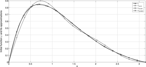
Figure 2. Exact and truncated solution for different δ with $\alpha =0.2$.

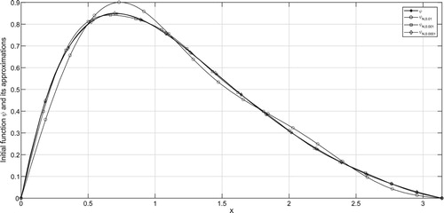
Figure 3. Exact and truncated solution for different δ with $\alpha =0.4$.

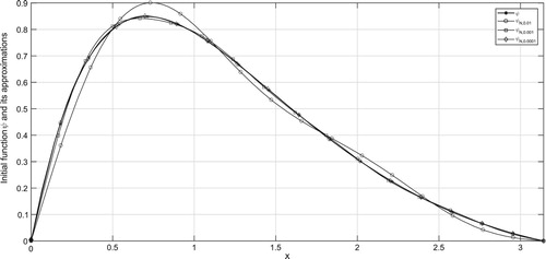
Figure 4. Exact and truncated solution for different δ with $\alpha =0.6$.

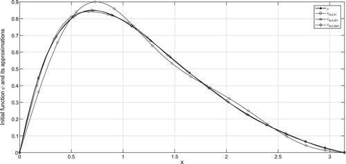
Figure 5. Exact and truncated solution for different δ with $\alpha =0.8$.

Figure 6. Exact and truncated solution for different δ with $\alpha =0.95$.

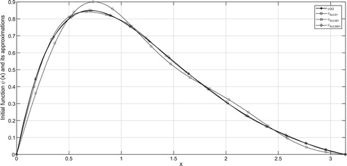
Figure 7. Exact and truncated solution for different δ with $\alpha =0.05$.

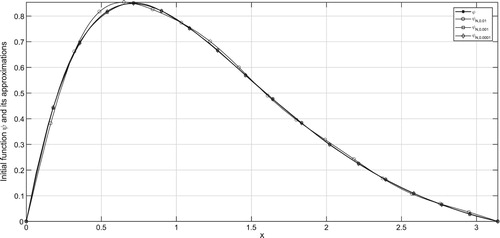
Figure 8. Exact and truncated solution for different δ with $\alpha =0.2$.

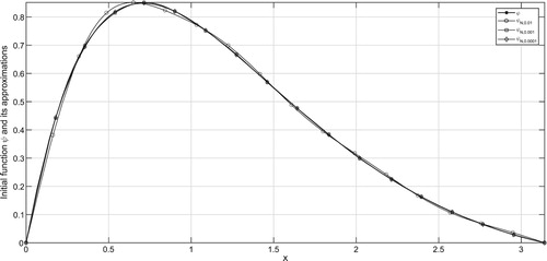
Figure 9. Exact and truncated solution for different δ with $\alpha =0.4$.

Figure 10. Exact and truncated solution for different δ with $\alpha =0.6$.

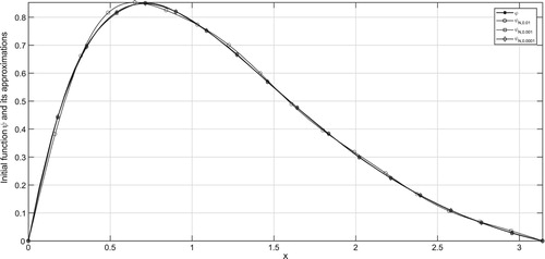
Figure 11. Exact and truncated solution for different δ with $\alpha =0.8$.

Figure 12. Exact and truncated solution for different δ with $\alpha =0.95$.

Table 1. Relative and absolute error estimates for different δ and α values.

	$\alpha =0.05$		$\alpha =0.2$		$\alpha =0.4$
δ	REE	AEE	REE	AEE	REE	AEE
0.01	0.0650	0.0075	0.0650	0.0075	0.0650	0.0075
0.001	0.0146	0.0017	0.0146	0.0017	0.0146	0.0017
0.0001	0.0039	4.524e-04	0.0039	4.524e-04	0.0039	4.524e-04

It can be seen from the figures that larger values of N result in stable solution and smaller values of N result with better approximations. From Tables 1 and 2, one can easily find that smaller values of α give better regularized solutions.

Table 2. Relative and absolute error estimates for different δ and α values.

	$\alpha =0.6$		$\alpha =0.8$		$\alpha =0.95$
δ	REE	AEE	REE	AEE	REE	AEE
0.01	0.0651	0.0075	0.0651	0.0075	0.0651	0.0075
0.001	0.0146	0.0017	0.0147	0.0017	0.0147	0.0017
0.0001	0.0040	4.5247e-04	0.0040	4.5247e-04	0.0040	4.5249e-04

Table 3. Relative and absolute error estimates for different δ and α values.

	$\alpha =0.05$		$\alpha =0.2$		$\alpha =0.4$
δ	REE	AEE	REE	AEE	REE	AEE
0.01	0.0200	0.0023	0.0201	0.0023	0.0206	0.0023
0.001	0.0057	6.5269e-04	0.0057	6.5343e-04	0.0057	6.5275e-04
0.0001	0.0013	1.5159e-04	0.0013	1.5159e-04	0.0013	1.5159e-04

Table 4. Relative and absolute error estimates for different δ and α values.

	$\alpha =0.6$		$\alpha =0.8$		$\alpha =0.95$
δ	REE	AEE	REE	AEE	REE	AEE
0.01	0.0202	0.0023	0.0201	0.0023	0.0200	0.0023
0.001	0.0057	6.5277e-04	0.0057	6.5372e-04	0.0057	6.5495e-04
0.0001	0.0013	1.5159e-04	0.0013	1.5159e-04	0.0013	1.5159e-04

Acknowledgements

The first author would like to acknowledge the support received from Indian Institute of Technology Madras and also the excellent facilities provided by the Department of Mathematics at Indian Institute of Technology Madras. Further, the authors thank the referees for their comments and suggestions which made the revised version better in many respects.

Disclosure statement

No potential conflict of interest was reported by the authors.

Additional information

Funding

This work was supported by the Indian Institute of Technology Madras through the Institute Woman Post-Doctoral Fellowship and also supported by the National Board for Higher Mathematics (Department of Atomic Energy, India) through the Post-Doctoral Fellowship [Grant No: 0204/15/2017/R&D-II/10380].

References

- Del Castillo Negrete D, Carreras BA, Lynch VE. Fractional diffusion in plasma turbulence. Phys Plasmas. 2004;11:3854–3864. doi: 10.1063/1.1767097
- Del Castillo Negrete D, Carreras BA, Lynch VE. Nondiffusive transport in plasma turbulence: a fractional diffusion approach. Phys Rev Lett. 2005;94:065–003. doi: 10.1103/PhysRevLett.94.065003
- Gorenflo R, Mainardi F, Moretti D, et al. Fractional diffusion: probability distributions and random walk models. Phys A Stat Mech Appl. 2002;305:106–112. doi: 10.1016/S0378-4371(01)00647-1
- Metzler R, Klafter J. The random walks guide to anomalous diffusion: a fractional dynamics approach. Phys Rep. 2000;339:1–77. doi: 10.1016/S0370-1573(00)00070-3
- Kneller G. Anomalous diffusion in biomolecular systems from the perspective of non-equilibrium statistical physics. Acta Phys Pol B. 2015;46:1167–1199. doi: 10.5506/APhysPolB.46.1167
- Nigmatullin RR. The realization of the generalized transfer equation in a medium with fractal geometry. Phys Status Solidi B. 1986;133:425–430. doi: 10.1002/pssb.2221330150
- Gorenflo R, Luchko Y, Mainardi F. Wright functions as scale-invariant solutions of the diffusion-wave equation. J Comput Appl Math. 2000;118:175–191. doi: 10.1016/S0377-0427(00)00288-0
- Gorenflo R, Luchko Y, Yamamoto M. Time-fractional diffusion equation in the fractional Sobolev spaces. Frac Calc Appl Anal. 2015;18:799–820.
- Kubica A, Yamamoto M. Initial-boundary value problems for fractional diffusion equations with time-dependent coefficients. Frac Calc Appl Anal. 2018;21:276–311. doi: 10.1515/fca-2018-0018
- Li Z, Liu Y, Yamamoto M. Initial-boundary value problems for multi-term time-fractional diffusion equations with positive constant coefficients. Appl Math Comput. 2015;257:381–397.
- Liu Y, Rundell W, Yamamoto M. Strong maximum principle for fractional diffusion equations and an application to an inverse source problem. Frac Calc Appl Anal. 2016;19:888–906.
- Luchko Y. Initial boundary value problems for the one dimensional time fractional diffusion equation. Frac Calc Appl Anal. 2012;15:141–160.
- Sakamoto K, Yamamoto M. Initial value boundary value problems for fractional diffusion wave equation and applications to some inverse problems. J Math Anal Appl. 2011;382:426–447. doi: 10.1016/j.jmaa.2011.04.058
- Cheng J, Nakagawa J, Yamamoto M, et al. Uniqueness in an inverse problem for a one dimensional fractional diffusion equation. Inverse Probl. 2009;25:115002. doi: 10.1088/0266-5611/25/11/115002
- Li Z, Yamamoto M. Uniqueness for inverse problems of determining orders of multi-term time fractional derivatives of diffusion equation. Appl Anal. 2015;94:570–579. doi: 10.1080/00036811.2014.926335
- Isakov V. Inverse problems for partial differential equations. Berlin: Springer-Verlag; 2006.
- Nair MT. Linear operator equation: approximation and regularization. Singapore: World Scientific; 2009.
- Liu JJ, Yamamoto M. A backward problem for the time fractional diffusion equation. Appl Anal. 2010;89:1769–1788. doi: 10.1080/00036810903479731
- Wang L, Liu J. Data regularization for a backward time fractional diffusion problem. Comput Math Appl. 2012;64:3613–3626. doi: 10.1016/j.camwa.2012.10.001
- Yang M, Liu J. Solving a final value fractional diffusion problem by boundary condition regularization. Appl Numer Math. 2013;66:45–58. doi: 10.1016/j.apnum.2012.11.009
- Wang JG, Wei T, Zhou YB. Tikhonov regularization method for a backward problem for the time-fractional diffusion equation. Appl Math Model. 2013;37:8518–8532. doi: 10.1016/j.apm.2013.03.071
- Wei T, Wang J. A modified quasi boundary value method for the backward time fractional diffusion problem. ESAIM Math Model Num. 2014;48:603–621. doi: 10.1051/m2an/2013107
- Zhang H, Zhang X. Generalized Tikhonov method for the final value problem of time-fractional diffusion equation. Int J Comput Math. 2017;94:66–78. doi: 10.1080/00207160.2015.1089354
- Tuan NH, Long LD, Nguyen VT, et al. On a final value problem for the time fractional diffusion equation with inhomogeneous source. Inverse Probl Sci En. 2016. doi:10.1080/17415977.2016.1259316.
- Tuan NH, Long LD, Tatar S. Tikhonov regularization method for a backward problem for the inhomogeneous time-fractional diffusion equation. Appl Anal. 2018;97:842–863. doi:10.1080/00036811.2017.1293815.
- Kilbas AA, Srivastava HM, Trujillo JJ. Theory and applications of fractional differential equations. Amsterdam: Elsevier; 2006.
- Podlubny I. Fractional differential equations. London: Academic Press; 1999.
- Wei T, Zhang ZQ. Robin coefficient identification for a time-fractional diffusion equation. Inverse Probl Sci Eng. 2014;24:647–666. doi: 10.1080/17415977.2015.1055261
- Rudin W. Principles of mathematical analysis. Singapore: McGraw-Hill; 1976.
- Kress R. Linear integral equations. 3rd ed New York: Springer; 2014.
- YX Zhang, Fu CL, Deng ZL. An a posteriori truncation method for some Cauchy problems associated with Helmholtz-type equations. Inverse Probl Sci Eng. 2013;21:1151–1168. doi: 10.1080/17415977.2012.743538