Damage identification in bridge structures subject to moving vehicle based on extended Kalman filter with l1-norm regularization

ABSTRACT

An innovative damage detection method for bridge structures under moving vehicular load is proposed on the basis of extended Kalman filter (EKF) and l1-norm regularization. An augmented state vector includes structural damage parameters and motion state variables of bridge and vehicle. Through a recursive process of the EKF, the structural damage parameters and state variables of a bridge are updated continually to obtain an optimal estimate using bridge responses due to a moving vehicle. The distribution of element stiffness reduction of a structure with local damages is sparse. Thus, l1-norm regularization is introduced into the updating process of the EKF using pseudo-measurement (PM) technology to improve the ill-posedness of the inverse problem. Numerical studies on a simple-supported and continuous beam bridge deck, with a smooth road surface that is subject to a moving vehicle, are performed to test the proposed approach. Furthermore, using the robustness of the EKF, the proposed algorithm is applied as a simplified method to the case where a bridge deck with road roughness is considered. Results show that the proposed identification algorithm is robust and effective for different vehicle speeds and measurement noises under smooth and good road conditions.

KEYWORDS:

• Damage identification
• moving vehicular
• extended Kalman filter
• l1-norm regularization
• pseudo-measurement

2010 MATHEMATICS SUBJECT CLASSIFICATIONS:

• 74H45
• 74H30
• 74P10

1. Introduction

Bridge structures undergo different levels of damages during their service lives given various natural hazards, aging, or overweight traffic loads. Monitoring any potential damage is an important means of improving the safety of bridge structures. Structural damages may change dynamic parameters, such as stiffness, mass, and damping, thereby reflecting the influence of damage in the vibration response of a bridge. In the past few decades, structure health monitoring and damage detection based on vibration responses have been an active research field [1–4].

In comparison with damage detection methods in time domain based on free or random vibration signals of bridges, an identification method based on traffic-induced bridge responses subject to moving vehicular loads is another important detection approach. A moving vehicle can be directly considered a convenient external load without any special equipment and is a perfect excitation source of larger responses than that under ambient vibration. Moreover, a dynamical model that considers a vehicle–bridge interaction can provide more reasonable dynamical response and enhance the accuracy of structural identification [5]. In recent years, damage detection approaches based on traffic-induced bridge responses have attracted considerable attention [6,7].

Damage detection techniques based on traffic-induced bridge responses can be categorized as signal- [8–10] and model-based methods [11–13]. In signal-based methods, different signal processing techniques, such as wavelet analysis [8,9] and Hilbert Huang transform (HHT) [14,15], are used for analyzing the dynamic responses of bridges directly. The singularity extracted from a bridge response signal can indicate the location and occurrence time of a structural damage. Meanwhile, model-based methods and model updating techniques are preferred for further quantifying a structural damage. A structural model provides a link between structural damage and vibration response; this model can be regarded as useful priori knowledge of structural damage identification. By minimizing the residuals between measured signals and reconstructed responses from the identified parameters, damage parameters are updated to detect the damage location and extent simultaneously in a model-based method. Recently, Lu [16] and Zhang [17] used a finite element model updating approach based on a dynamic response sensitivity to identify structural damages and vehicular parameters. The solution was obtained iteratively using a penalty function method with Tikhonov regularization. Li and Law [18] proposed a damage identification approach for bridge structures under moving vehicular loads without knowledge of vehicle properties and time histories of moving interaction forces. Feng [19] presented a finite element model updating approach to monitor an aging railway bridge using in situ dynamic displacement measurements under trainloads. Given that the structural response and sensitivity of all time points are required to establish an input–output relationship, the main drawback of this approach is that it is time-consuming, thereby limiting its application to structural on-line damage identification.

As a recursive model updating method, extended Kalman filter (EKF) is another effective tool for damage detection. The EKF has been extensively applied to damage identification given its favourable performance in arithmetic robustness, identification accuracy, and fast convergence [20–23]. Yang et al. [24,25] combined the EKF and adaptive fading forgetting factor to identify the changes in structural parameters online. To reduce the order of the system state vector of large and complex structures, the substructure approach [26,27] can be introduced in the EKF algorithm for the damage identification of complex structures. In theory, EKF is feasible and effective for parameter identification in time-varying vehicle–bridge systems considering mass distribution changes. Therefore, studies must be conducted to develop an EKF algorithm for damage identification in bridge structures subjected to moving vehicles.

Damage identification of bridge structures is a typical ill-condition problem. Regularization technology [28,29] is a major and effective method for alleviating the ill-posedness of an inverse problem by solving an approximate well-posed problem. Tikhonov regularization, the most extensively used l2-norm regularization, can be introduced conveniently to the EKF algorithm [30]. However, the l2-norm-based regularization method obtains an approximate solution by blurring the singularity of the real solution in the original problem [31,32]. An over-smooth solution is inconsistent with structural local damages because local damage cases have few element stiffness changes, and the distribution of damage parameters is sparse. Recently, the concept of sparsity has been applied to structural health monitoring in the form of l1-norm regularization [33–35]. Studies have shown that sparse regularization is superior to the classical sensitivity method for structural local damages. Therefore, the method developed herein combines the l1-regulation norm process to improve the ill-posedness of the damage identification problem in time-varying vehicle–bridge interaction (VBI) systems.

In this work, the bridge is modelled as a Euler–Bernoulli beam with a smooth road surface, and the vehicle is modelled as a moving oscillator with four parameters. On the basis of a bridge's vibration responses caused by a passing vehicle, an improved EKF algorithm with l1-norm regularization is used to identify the local bridge damages in accordance with the sparse characteristics of damage parameters. A simply supported bridge and a multi-span continuous bridge are studied as two numerical examples to demonstrate the correctness and efficiency of the proposed algorithm. The effects of different measurements, such as noise, vehicle weight, vehicle speed, signal type, and bridge type, on the identification results are investigated. Furthermore, the proposed EKF algorithm is applied as a simplified method to the case where the bridge deck with road roughness is considered using the robustness of the EKF. This work indicates that the proposed algorithm is computationally stable and efficient for local damage identification under good road conditions.

2. Dynamic equations of the VBI system

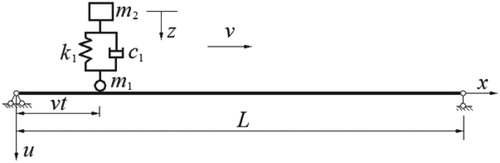
A vibration analysis of VBI system is a classical dynamics problem. Vehicle and bridge systems are coupled through the interaction forces and the compatibility of displacements at the contact points without considering the separation of the vehicle and the bridge deck.

In this work, the bridge is assumed as a linear elastic Bernoulli–Euler beam with the following properties: mass per unit length $m$, flexural rigidity $EI\left(x\right)$, bridge length $L$, and damping $c$. The moving vehicle is modelled as an oscillator with four parameters, namely, unsprung mass $m_1$, sprung mass $m_2$, spring stiffness $k_1$, and damping coefficient $c_1$. The vertical displacement of sprung mass $m_2$ is denoted by $z\left(t\right)$, and the displacement of the bridge at a horizontal position $x$ is represented by $u\left(x,t\right)$. The contact surface between the bridge and the oscillator is smooth, and the oscillator that moves at a constant speed $v$ is assumed to remain in contact with the bridge surface. On the basis of the abovementioned assumptions and dynamic equilibrium, the motion equations of the vehicle–bridge interaction model illustrated in Figure 1 can be derived as (1a) $m_2\ddot{z}\left(t\right)+k_1\left[z\left(t\right)-{u\left(x,t\right)|}_{x=vt}\right]+c_1\left[\dot{z}\left(t\right)-{\left.\frac{\mathrm{\partial }u\left(x,t\right)}{\mathrm{\partial }t}\right|}_{x=vt}\right]=0,$(1a) (1b) $m\frac{{\mathrm{\partial }}^{2}u\left(x,t\right)}{\mathrm{\partial }{t}^2}+c\frac{\mathrm{\partial }u\left(x,t\right)}{\mathrm{\partial }t}+\frac{{\mathrm{\partial }}^2}{\mathrm{\partial }{x}^2}\left[EI\left(x\right)\frac{{\mathrm{\partial }}^{2}u\left(x,t\right)}{\mathrm{\partial }{x}^2}\right]=\delta \left(x-vt\right)f_c\left(x,t\right),$(1b) where the contact force $f_c\left(x,t\right)$ between the vehicle and the bridge can be written as $f_c\left(x,t\right)=\left(m_1+m_2\right)g-m_1\frac{{\mathrm{\partial }}^{2}u\left(x,t\right)}{\mathrm{\partial }{t}^2}+k_1\left[z\left(t\right)-u\left(x,t\right)\right]+c_1\left[\dot{z}\left(t\right)-\frac{\mathrm{\partial }u\left(x,t\right)}{\mathrm{\partial }t}\right].$ Through a normal-mode method, the vibration response of the bridge can be represented as (2) $u\left(x,t\right)=\sum _{i=1}^N{p}_i\left(t\right){\phi }_i\left(x\right)=\mathit{\phi }\mathit{p},$(2) where $N$ is the number of truncated modes, $\mathit{\phi }=\left[\begin{array}{ccc}{\phi }_1\left(x\right)& \cdots & {\phi }_N\left(x\right)\end{array}\right]$, and ${\phi }_i\left(x\right)$ is the ith mass normalized mode shape, $\mathit{p}={\left[\begin{array}{ccc}{p}_1\left(t\right)& \cdots & p_N\left(t\right)\end{array}\right]}^T$, and $p_i\left(t\right)$ is the ith general modal coordinate. The substitution of Equation (2) into Equation (1) and application of the orthogonality conditions yield the VBI system motion equation as follows: (3) $\mathit{M}\ddot{\mathit{q}}+\mathit{C}\dot{\mathit{q}}+\mathit{K}\mathit{q}=\mathit{F},$(3) where $\mathit{q}={\left[\begin{array}{cccc}{p}_1& \cdots & p_N& z\end{array}\right]}^T$ is the generalized displacement vector; $\mathit{M},\mathit{C},$ and $\mathit{K}$ denote the generalized mass, damping, and stiffness matrices, respectively; and $\mathit{F}$ is the generalized force vector. (4a) $\mathit{M}=\left[\begin{array}{ccccc}1+m_1{\Phi }_{11}& m_1{\Phi }_{12}& \cdots & m_1{\Phi }_{1N}& 0\\ m_1{\Phi }_{21}& 1+m_1{\Phi }_{22}& \cdots & m_1{\Phi }_{2N}& 0\\ ⋮& ⋮& \cdots & ⋮& ⋮\\ m_1{\Phi }_{N1}& m_1{\Phi }_{N2}& \cdots & 1+m_1{\Phi }_{NN}& 0\\ 0& 0& \cdots & 0& m_2\end{array}\right],$(4a) (4b) $\mathit{C}=\left[\begin{array}{ccccc}2{\xi }_1{\omega }_1+c_1{\Phi }_{11}& c_1{\Phi }_{12}& \cdots & c_1{\Phi }_{1N}& -c_1{\phi }_1\left(vt\right)\\ c_1{\Phi }_{21}& 2{\xi }_2{\omega }_2+c_1{\Phi }_{22}& \cdots & c_1{\Phi }_{2N}& -c_1{\phi }_2\left(vt\right)\\ ⋮& ⋮& \cdots & ⋮& ⋮\\ c_1{\Phi }_{N1}& c_1{\Phi }_{N2}& \cdots & 2{\xi }_N{\omega }_N+c_1{\Phi }_{NN}& -c_1{\phi }_N\left(vt\right)\\ -c_1{\phi }_1\left(vt\right)& -c_1{\phi }_2\left(vt\right)& \cdots & -c_1{\phi }_N\left(vt\right)& c_1\end{array}\right],$(4b) (4c) $\mathit{K}=\left[\begin{array}{ccccc}{\omega }_1^2+k_1{\Phi }_{11}& k_1{\Phi }_{12}& \cdots & k_1{\Phi }_{1N}& -k_1{\phi }_1\left(vt\right)\\ k_1{\Phi }_{21}& {\omega }_2^2+k_1{\Phi }_{22}& \cdots & k_1{\Phi }_{2N}& -k_1{\phi }_2\left(vt\right)\\ ⋮& ⋮& \cdots & ⋮& ⋮\\ k_1{\Phi }_{N1}& k_1{\Phi }_{N2}& \cdots & {\omega }_N^2+k_1{\Phi }_{NN}& -k_1{\phi }_N\left(vt\right)\\ -k_1{\phi }_1\left(vt\right)& -k_1{\phi }_2\left(vt\right)& \cdots & -k_1{\phi }_N\left(vt\right)& k_1\end{array}\right],$(4c) (4d) $\mathit{F}=\left(m_1+m_2\right)g{\left[\begin{array}{ccccc}{\phi }_1\left(vt\right)& {\phi }_2\left(vt\right)& \cdots & {\phi }_n\left(vt\right)& 0\end{array}\right]}^T,$(4d) where ${\omega }_i$ is the ith undamped natural frequency, ${\xi }_i$ is the ith modal damping ratio, and ${\Phi }_{ij}={\phi }_i\left(vt\right){\phi }_j\left(vt\right)$, $i,j=1,\cdots ,N$. When the vehicle moves on the bridge, the coefficient matrices $\mathit{M}$, $\mathit{C},$ and $\mathit{K}$ in dynamics Equation (3) will change continuously with time.

Figure 1. The vehicle–bridge interaction system.

3. EKF for structural damage identification based on VBI responses

3.1. Nonlinear model of vehicle -bridge interaction vibration in EKF frame

Kalman filter (KF) is a linear optimal recursive estimator designed for linear time-varying dynamic systems and thus is particularly suitable for system identification of the VBI system. To estimate the structural parameters, the state vector of the KF is extended. Then, the EKF is proposed for the corresponding nonlinear system identification as the nonlinear version of the KF.

In structural damage identification problems, the EKF method must identify the system state and structural parameters simultaneously. Therefore, the extended state vector of the system is defined in this work as (5) $\mathit{\theta }=[\mathit{q}\left(t\right)\dot{\mathit{q}}\left(t\right)\mathit{\alpha }{]}^T,$(5) where $\mathit{\alpha }=\left[{\alpha }_1\cdots {\alpha }_{ne}\right]$ is the change of the element stiffness, and $ne$ is the number of elements. Herein, on the basis of an initial finite element model of the undamaged structure, the element damage parameter ${\alpha }_i$ is defined as (6) ${\alpha }_i=1-E_i/E_i^0,$(6) where $E_i^0$ and $E_i$ correspond to the initial and current elastic modulus values of the ith element. In the definition of a state vector, the concept of structural modal truncation is used to reduce the dimension of the state vector effectively because the bridge structure response mainly contains low-order modal components.

Considering that the element damage parameters are constant, the dynamics Equation (3) can be written as the corresponding state space formulation. (7) $\dot{\mathit{\theta }}\left(t\right)=\left[\begin{array}{c}\dot{\mathit{q}}\left(t\right)\\ \ddot{\mathit{q}}\left(t\right)\\ \dot{\mathit{\alpha }}\end{array}\right]=\left[\begin{array}{c}\dot{\mathit{q}}\left(t\right)\\ {\mathit{M}}^{-1}\left(\mathit{F}\left(t\right)-\mathit{C}\dot{\mathit{q}}\left(t\right)-\mathit{K}\mathit{q}\left(t\right)\right)\\ 0_{1\times ne}\end{array}\right]=\mathit{f}\left(\mathit{\theta },t\right).$(7) In accordance with Equations (2) and (7), the corresponding state and observation equations of the EKF can be represented as (8) $\dot{\mathit{\theta }}\left(t\right)=f\left(\mathit{\theta },t\right)+\mathit{W},$(8) (9) $\mathit{y}\left(\mathit{x},t\right)=h\left(\mathit{\theta }\left(t\right),\mathit{x},t\right)+\mathit{V},$(9) where $\mathit{y}\left(\mathit{x},t\right)$ are the measured quantities (displacements, velocities, and accelerations) at measurement point $\mathit{x}$; $\mathit{W}$ and $\mathit{V}$ correspond to the process and observation noises, which are assumed to be zero mean multivariate Gaussian noises with covariances $\mathit{Q}$ and $\mathit{R}$, respectively; and response function $\mathit{h}\left(\mathit{\theta }\left(t\right),\mathit{x},t\right)$ has different expressions that depend on the type of observation data. (10) $\mathit{h}\left(\mathit{\theta }\left(t\right),\mathit{x},t\right)=\left\{\begin{array}{ll}\phi \mathit{p}\left(t\right),& \text{if the observation is displacement response}\\ \phi \dot{\mathit{p}}\left(t\right),& \text{if the observation is velocity response}\\ \phi \ddot{\mathit{p}}\left(t\right),& \text{if the observation is acceleration response}\end{array}\right..$(10) Since the nonlinear coupling of state variables $\mathit{q}$ and $\dot{\mathit{q}}$ with structural parameters $\mathit{\alpha }$, the estimation problem becomes nonlinear even if a bridge structure and a vehicle model are linear. The EKF adapts multivariate Taylor series expansions to linearize the state transition and observation equations around the previous state estimate; thus, the following discretized and linearized recursive equations at a time $t_k$ can be obtained in accordance with the standard EKF algorithm [36]. (11) ${\tilde{\mathit{\theta }}}_{k+1}={\hat{\mathit{\theta }}}_k+\underset{k\mathrm{\Delta }t}{\overset{\left(k+1\right)\mathrm{\Delta }t}{\int }}f\left(\mathit{\theta }\left(t\right),t\right)\text{d}t,$(11) (12) ${\tilde{\mathit{P}}}_{k+1}={\mathit{A}}_k{\hat{\mathit{P}}}_k{\mathit{A}}_k^{\mathit{T}}+{\mathit{Q}}_k\text{ },$(12) (13) ${\mathit{K}}_{k+1}={\tilde{\mathit{P}}}_{k+1}{\mathit{H}}_{k+1}^T\left({\mathit{H}}_{k+1}{\hat{\mathit{P}}}_{k+1}{\mathit{H}}_{k+1}^T+{\mathit{R}}_{k+1}\right){}^{-1},$(13) (14) ${\hat{\mathit{\theta }}}_{k+1}={\tilde{\mathit{\theta }}}_{k+1}+{\mathit{K}}_{k+1}\left({\mathit{y}}_{k+1}-h\left({\tilde{\mathit{\theta }}}_{k+1}\right)\right),$(14) (15) ${\hat{\mathit{P}}}_{k+1}=\left(\mathit{I}-{\mathit{K}}_{k+1}{\mathit{H}}_{k+1}\right){\tilde{\mathit{P}}}_{k+1},$(15) where ${\hat{\mathit{\theta }}}_k$ is the state estimate vector of ${\mathit{\theta }}_k$ at time step$\text{ }k$, ${\tilde{\mathit{\theta }}}_{k+1}$ is the prediction of the state vector at time step $k+1$, ${\hat{\mathit{P}}}_k$ is the covariance matrix of the estimation error associated with the updated estimate ${\hat{\mathit{\theta }}}_k$, ${\tilde{\mathit{P}}}_{k+1}$ is the covariance matrix of the estimation error associated with the prior estimate ${\tilde{\mathit{\theta }}}_{k+1}$, $\mathrm{\Delta }t$ is the time step, and ${\mathit{K}}_{k+1}$ is the Kalman gain matrix. Here, the state transition matrix $\mathit{A}$ and measurement matrix $\mathit{H}$ required in the EKF algorithm are calculated by discretizing and linearizing Equations (8) and (9). (16) $\mathit{A}=\mathit{I}+{\left.\frac{\mathrm{\partial }f\left(\mathit{\theta },t\right)}{\mathrm{\partial }\mathit{\theta }}\right|}_{\mathit{\theta }={\mathit{\theta }}_k}\mathrm{\Delta }t=\mathit{I}+{\left.\left[\begin{array}{ccc}\frac{\mathrm{\partial }f}{\mathrm{\partial }\mathit{q}}& \frac{\mathrm{\partial }f}{\mathrm{\partial }\dot{\mathit{q}}}& \frac{\mathrm{\partial }f}{\mathrm{\partial }\mathit{\alpha }}\end{array}\right]\right|}_{\mathit{\theta }={\mathit{\theta }}_k}\mathrm{\Delta }t,$(16) where $\begin{array}{ccc}\frac{\mathrm{\partial }\mathit{f}}{\mathrm{\partial }\mathit{q}}=\left[\begin{array}{c}0\\ -\mathit{L}\\ 0\end{array}\right],& \frac{\mathrm{\partial }\mathit{f}}{\mathrm{\partial }\dot{\mathit{q}}}=\left[\begin{array}{c}\mathit{I}\\ -\mathit{B}\\ 0\end{array}\right],& \frac{\mathrm{\partial }\mathit{f}}{\mathrm{\partial }\mathit{\alpha }}=\left[\begin{array}{c}0\\ -\frac{\mathrm{\partial }\mathit{L}}{\mathrm{\partial }\mathit{\alpha }}\mathit{q}-\frac{\mathrm{\partial }\mathit{B}}{\mathrm{\partial }\mathit{\alpha }}\dot{\mathit{q}}+\frac{\mathrm{\partial }{\mathit{F}}_f}{\mathrm{\partial }\mathit{\alpha }}\\ 0\end{array}\right]\end{array},$ $\mathit{B}={\mathit{M}}^{-1}\mathit{C},\mathit{L}={\mathit{M}}^{-1}\mathit{K},{\mathit{F}}_f={\mathit{M}}^{-1}\mathit{F}.$ The measurement matrix $\mathit{H}$ has the following form (17a) $\mathit{H}={\left.\frac{\mathrm{\partial }h\left(\mathit{\theta },\mathit{x},t\right)}{\mathrm{\partial }\mathit{\theta }}\right|}_{\mathit{\theta }={\mathit{\theta }}_k}={\left.\left[\begin{array}{ccc}\frac{\mathrm{\partial }h}{\mathrm{\partial }\mathit{q}}& \frac{\mathrm{\partial }h}{\mathrm{\partial }\dot{\mathit{q}}}& \frac{\mathrm{\partial }h}{\mathrm{\partial }\mathit{\alpha }}\end{array}\right]\right|}_{\mathit{\theta }={\mathit{\theta }}_k}$(17a) (17b) $\begin{array}{cc}=\left[\begin{array}{ccc}\left[\begin{array}{cc}\phi & 0\end{array}\right]& 0& \left[\begin{array}{cc}\frac{\mathrm{\partial }\phi }{\mathrm{\partial }\mathit{\alpha }}\mathit{p}& 0\end{array}\right]\end{array}\right]& \left(\text{if}\mathit{y}=\phi \mathit{p}\left(t\right)\right)\end{array}$(17b) (17c) $\begin{array}{cc}=\left[\begin{array}{ccc}0& \left[\begin{array}{cc}\phi & 0\end{array}\right]& \left[\begin{array}{cc}\frac{\mathrm{\partial }\phi }{\mathrm{\partial }\mathit{\alpha }}\dot{\mathit{p}}& 0\end{array}\right]\end{array}\right]& \left(\text{if}\mathit{y}=\phi \dot{\mathit{p}}\left(t\right)\right)\end{array}$(17c) (17d) $\begin{array}{rl}& =\left[\begin{array}{ccc}\left[\begin{array}{cc}-\phi {\mathit{H}}_a\mathit{L}& 0\end{array}\right]& \left[\begin{array}{cc}-\phi {\mathit{H}}_a\mathit{B}& 0\end{array}\right]& \frac{\mathrm{\partial }\phi }{\mathrm{\partial }\mathit{\alpha }}{\mathit{H}}_a\ddot{\mathit{q}}+\phi {\mathit{H}}_a\left(\frac{\mathrm{\partial }{\mathit{F}}_f}{\mathrm{\partial }\mathit{\alpha }}-\frac{\mathrm{\partial }\mathit{B}}{\mathrm{\partial }\mathit{\alpha }}\dot{\mathit{q}}-\frac{\mathrm{\partial }\mathit{L}}{\mathrm{\partial }\mathit{\alpha }}\mathit{q}\right)\end{array}\right]\\ & \left(\text{if}\mathit{y}=\phi \ddot{\mathit{p}}\left(t\right)\right)\end{array}$(17d) Where ${\mathit{H}}_a=\left[\begin{array}{cc}{\mathit{I}}_{N\times N}& 0_{N\times 1}\end{array}\right]$, and the derivation processes of $\frac{\mathrm{\partial }\mathit{L}}{\mathrm{\partial }{\alpha }_i},\frac{\mathrm{\partial }\mathit{B}}{\mathrm{\partial }{\alpha }_i}$, and $\frac{\mathrm{\partial }{\mathit{F}}_f}{\mathrm{\partial }{\alpha }_i}$ are demonstrated in the Appendix section. If we assume that bridge damages only affect structural stiffness and not the structural mass, the sensitivity of nature frequencies and modes to damage parameters, $\mathrm{\partial }{\omega }_n/\mathrm{\partial }{\alpha }_i$ and $\mathrm{\partial }{\phi }_n/\mathrm{\partial }{\alpha }_i$, in $\mathit{A}$ and $\mathit{H}$ can be expressed as [28] (18) $\begin{array}{cc}\frac{\mathrm{\partial }{\mathit{\omega }}_i}{\mathrm{\partial }{\mathit{\alpha }}_j}=-\frac{1}{2{\omega }_i}{\phi }_i^T{\mathit{K}}_{j0}^e{\phi }_i,& \frac{\mathrm{\partial }{\phi }_i}{\mathrm{\partial }{\mathit{\alpha }}_j}=\sum _{r,r\ne i}\frac{{\phi }_r^T{\mathit{K}}_{j0}^e{\phi }_i}{{\omega }_r^2-{\omega }_i^2}{\phi }_r\end{array},$(18) where ${\mathit{K}}_{j0}^e$ is the element stiffness matrix in undamaged model. It should be noted that the Equation (11) can be solved by numerical integration methods, such as Newmark-beta or Wilson-theta methods.

Prior to EKF recursion, the initial values of the state vector ${\hat{\mathit{\theta }}}_0$ and error covariance matrix ${\hat{\mathit{P}}}_0$ of the initial estimation are required. Appropriate initial values of the state vector and covariance matrix help improve the convergence of the algorithm. However, for a stable EKF process, the initial value of the state vector slightly affects the convergence of the algorithm. Thus, the precision of the preset initial value can be relaxed. This phenomenon is an advantage of the EKF method used in damage identification based on structural time-history responses. This advantage indicates that structural damage can be identified in the absence of an accurate initial state.

In each recursive step, the modal parameters (eigenfrequencies and mode shapes) can be calculated using the current damage parameters through the sensitivity method, and then the predicted values of the structural response can be obtained using the dynamic equations and through the mode superposition method. By comparing the difference between the observed and measured responses, the EKF algorithm can continuously update the state vector and obtain the optimal estimate of structural damages.

3.2. Modified EKF algorithm with l1-norm regularization

For the system described in Equations (8) and (9), the classical EKF algorithm provides an optimal or suboptimal estimate ${\hat{\mathit{\theta }}}_k$ with a minimal mean square error, which is a solution to the unconstrained l2-norm minimization problem. (19) $\underset{{\hat{\mathit{\theta }}}_k}{min}{\mathit{E}}_{{\mathit{\theta }}_k|{\mathit{y}}_k}\left[||{\mathit{\theta }}_k-{\hat{\mathit{\theta }}}_k|{|}_2^2\right],$(19) When the optimal solution of the KF algorithm is understood from the perspective of Bayesian inference, KF has a certain self-regularization ability, and a maximum a posteriori (MAP) estimation is equivalent to a least square solution with an l2 regularization item. However, an optimal estimation with minimum variance is still expected, and the weights of measurement and prior information are difficult to adjust in the KF algorithm actively. Therefore, a special and additional regularization process is introduced into the EKF algorithm to obtain the ideal damage identification effect. For a structure with local damages, the distribution of damage parameters is sparse because most of the damage parameters (${\alpha }_i$) are zero, and only a few parameters are non-zero. The l1-norm regularization process has been confirmed superior to the traditional l2-norm regularization in preserving the sparseness of results. After considering the l1-norm regularization, the optimization problem is modified as (20) $\underset{{\hat{\mathit{\theta }}}_k}{min}{\mathit{E}}_{{\mathit{\theta }}_k|{\mathit{y}}_k}\left[||{\mathit{\theta }}_k-{\hat{\mathit{\theta }}}_k|{|}_2^2+\gamma {||\mathit{\alpha }||}_1\right],$(20) where $||\mathit{\alpha }|{|}_1=\sum _i|{\alpha }_i|$ is the l1-norm of the vector, and $\gamma$ is the l1-norm regulation parameter. To obtain the solution within the framework of the EKF algorithm, the l1-norm minimization problem (20) can be replaced with the following constrained optimization [37]: (21) $\begin{array}{cc}\underset{{\hat{\mathit{\theta }}}_k}{min}{\mathit{E}}_{{\mathit{\theta }}_k|{\mathit{y}}_k}\left[||{\mathit{\theta }}_k-{\hat{\mathit{\theta }}}_k|{|}_2^2\right],& \text{s}.\text{t}.{||\mathit{\alpha }||}_1<\epsilon \end{array}$(21) where $\epsilon$ is a sufficiently small value, and then a so-called pseudo-measurement (PM) technique [38] is used to incorporate the l1-norm conditions into the EKF filtering process.

The PM method replaces the inequality constraints $||\mathit{\alpha }|{|}_1<\mathit{\epsilon }$ by adding a fictitious measurement update procedure in each EKF recursive step. The PM process is also a KF process, and the state and fictitious measurement equations are (22) ${\mathit{\theta }}_k={\mathit{\theta }}_{k-1},$(22) (23) $0=\overline{\mathit{H}}\cdot {\mathit{\theta }}_k-\epsilon ,$(23) where $\overline{\mathit{H}}=\left[\begin{array}{cccccc}{0}_{1\times N},& 0_{1\times N},& \text{sign}\left({\alpha }_1\right),& \cdots ,& \text{sign}\left({\alpha }_{ne}\right),& 0_{1\times N}\end{array}\right]$, and ${\mathit{\theta }}_k$ is the state vector in time step $k$. Here, $\text{sign}\left({\alpha }_i\right)$ denotes the sign function of damage parameter ${\alpha }_i$. (24) $\text{sign}\left({\alpha }_i\right)=\left\{\begin{array}{ll}1,& \text{if}{\alpha }_i\ge 0\\ -1,& \text{if}{\alpha }_i<0\end{array}\right.$(24) The PM method must be understood in the statistical framework of KF. The state Equation (22) provides a one-step prediction vector, and the corresponding covariance matrix provides different prediction errors of each damage parameter. In the fictitious measurement Equation (23), the fictitious observation value is always 0, which means that $||\mathit{\alpha }|{|}_1=\overline{\mathit{H}}\cdot {\mathit{\theta }}_k$ and fictitious measurement noise $\epsilon$ has the same mean and variance. Here, the measurement noise $\epsilon$ is a normal random variable with a zero mean and variance$\text{ }{R}_{\epsilon }$. When the predicted observation $||\mathit{\alpha }|{|}_1=\overline{\mathit{H}}\cdot {\mathit{\theta }}_k$ deviates from the fictitious observation value 0, the state vector is updated in accordance with the Kalman filtering algorithm by combining the prediction and observation errors. Then, the recursive update process will cause the norm $||\mathit{\alpha }|{|}_1$ to gradually decrease and approach the fictitious observation value 0, especially when the variance is small. Evidently, a small$\text{ }{R}_{\epsilon }$ implies a strong l1-norm constraint, thereby leading to poor structural response estimates and improved damage parameter estimates. Subsequently, a large $R_{\epsilon }$ relaxes the l1-norm constraint and obtains improved structural response estimates and poor damage parameter estimates. As a tuning parameter for controlling the tightness of the l1-norm constraint, the role of $R_{\epsilon }$ is similar to the regularization parameter $\gamma$ in the classical regularization method, as expressed in Equation (20); thus, L-curve method [39] can be used to determine the covariance $R_{\epsilon }$ as a well-known method for selecting regularization parameters. For different covariance $R_{\epsilon }$ values, various estimates of the state vector $\hat{\mathit{\theta }}$ and structural response $\hat{\mathit{y}}=h\left(\hat{\mathit{\theta }},\mathit{x},t\right)$ can be obtained. The l1-norm of the regularized identification results $||\mathit{\alpha }|{|}_1$ versus the norm of the corresponding response residual vector$||\hat{\mathit{y}}-\mathit{y}|{|}_2^2$ is convenient to plot. Finally, the value of covariance $R_{\epsilon }$ is decided by finding a regularized solution near the L-shaped corner of the L-curve.

In accordance with the damage identification method based on the VBI responses and the PM technique, the proposed EKF method with l1-norm regularization in damage identification is summarized in Algorithm 1.

Table

Algorithm 1:
In each recursive step of EKF
1: Prediction Update
	${\tilde{\mathit{\theta }}}_{k+1}={\hat{\mathit{\theta }}}_k+\underset{k\mathrm{\Delta }t}{\overset{\left(k+1\right)\mathrm{\Delta }t}{\int }}f\left(\mathit{\theta }\left(t\right),t\right)\text{d}t$
	${\tilde{\mathit{P}}}_{k+1}={\mathit{A}}_k{\hat{\mathit{P}}}_k{\mathit{A}}_k^{\mathit{T}}+{\mathit{Q}}_k$
2: Measurement Update
	${\mathit{K}}_{k+1}={\tilde{\mathit{P}}}_{k+1}{\mathit{H}}_{k+1}^T\left({\mathit{H}}_{k+1}{\hat{\mathit{P}}}_{k+1}{\mathit{H}}_{k+1}^T+{\mathit{R}}_{k+1}\right){}^{-1}$
	${\hat{\mathit{\theta }}}_{k+1}={\tilde{\mathit{\theta }}}_{k+1}+{\mathit{K}}_{k+1}\left({\mathit{y}}_{k+1}-h\left({\tilde{\mathit{\theta }}}_{k+1}\right)\right)$
	${\hat{\mathit{P}}}_{k+1}=\left(\mathit{I}-{\mathit{K}}_{k+1}{\mathit{H}}_{k+1}\right){\tilde{\mathit{P}}}_{k+1}$
3: Pseudo Measurement Update:
Let  ${\mathit{P}}^1={\hat{\mathit{P}}}_{k+1}$  and  ${\hat{\mathit{\theta }}}^1={\hat{\mathit{\theta }}}_{k+1}$
for  $\tau =1,2,\cdots ,N_{\tau }-1$  iterations  do
	${\overline{\mathit{H}}}_{\tau }=\overline{\mathit{H}}\left({\hat{\mathit{\theta }}}^{\tau }\right)$	(25)
	${\mathit{G}}^{\tau }={\mathit{P}}^{\tau }{\overline{\mathit{H}}}_{\tau }^T({\mathit{H}}_{\tau }{\mathit{P}}^{\tau }{\mathit{H}}_{\tau }^T+{\mathit{R}}_{\epsilon }{)}^{-1}$	(26)
	${\hat{\mathit{\theta }}}^{\tau +1}=\left(\mathit{I}-{\mathit{G}}^{\tau }{\overline{\mathit{H}}}_{\tau }\right){\hat{\mathit{\theta }}}^{\tau }$	(27)
	${\mathit{P}}^{\tau +1}=\left(\mathit{I}-{\mathit{G}}^{\tau }{\overline{\mathit{H}}}_{\tau }\right){\mathit{P}}^{\tau }$	(28)
end for
Set  ${\hat{\mathit{P}}}_{k+1}={\mathit{P}}^{N_{\tau }}$, ${\hat{\mathit{\theta }}}_{k+1}={\hat{\mathit{\theta }}}^{N_{\tau }}$

where the number of PM iterations $N_{\tau }$ is artificially selected to balance the estimation accuracy and computational complexity. Generally, $N_{\tau }=10$ is sufficient.

4. Numerical example of damage identification

4.1. Example1: simply-supported bridge

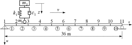
To investigate the performance of the proposed damage detection algorithm for bridge structures, a numerical example of a simply supported bridge [40] subject to a moving vehicle is studied. The physical parameters of the bridge are presented as follows: length of 36 m, $EI=2.3\times {10}^{10}\text{N}{\text{m}}^2$, mass density of $5\times {10}^3\text{kg/m}$, and modal damping ratio of 0.02. The bridge is divided evenly into 10 Euler–Bernoulli beam elements with 11 nodes, as depicted in Figure 2, and the structural damage is simulated by a reduction in the elastic modulus of the element. The moving vehicle is modelled as a four-parameter oscillator [41] with the following parameters: $m_1=3000\text{kg}$, $m_2=31700\text{kg}$, $k_1=9.12\times {10}^6\text{N/m}$, and $c_1=86000\text{Ns/m}$. The vertical vibrations of the vehicle and the bridge are set to 0 before the vehicle enters the bridge. When the vehicle passes through the bridge at a constant speed $v$, the vertical displacements of 2–10 nodes on the bridge are measured for damage identification. The sampling frequency of the vibration signals is 1000 Hz. Gaussian white noise $\mathit{ϵ}\left(t\right)$ is added to the original vibration signals $\tilde{\mathit{y}}$ to simulate the actual measurement$\text{ }\mathit{y}$. (29) $\mathit{y}\left(t\right)=\tilde{\mathit{y}}\left(t\right)+\mathit{ϵ}\left(t\right).$(29) Here, the level of measurement noise $\mathit{ϵ}\left(t\right)$ is represented by the signal-to-noise ratio (SNR) of dB, where $\text{SNR}=10\times \text{lg}\left(SP\text{/}NP\right)$, $SP$ is the signal power, and $NP$ is the noise power. In addition, the bridge structural responses mainly include the first three modal components in accordance with the structural dynamic calculation; therefore, the generalized modal coordinate number in the system state vector is 3 in all numerical examples.

Figure 2. The models of the moving vehicle and the simple-supported bridge.

Different factors that influence the accuracy of the identified result must be examined. Herein, the effects of damage location and extent, the measurement noise, measurement point number, measurement signal type, vehicle speed, and vehicle weight are studied.

4.1.1. Damage identification in different damage cases

Two local damage cases, that is, single and multiple damages, are studied to investigate the effect of damage location and extent on the identification results, as summarized in Table 1. In the two cases, vehicle speed $v$ is set to $20\text{m/s}$, and three noise levels (20, 25, and 30 dB) are considered.

Table 1. Two local damage cases of the simply-supported beam bridge.

	Case1	Case2
Damage element	5	2	5	7
Damage parameter	30%	15%	30%	20%

To determine the appropriate covariance ($R_{\mathit{\epsilon }}$) of the proposed identification algorithm, Figure 3 plots the L-curve of the observed residual norm and the regularized solution norm as described in Section 3.2. Then, the optimal value of covariance $R_{\epsilon }$ can be determined by the corner of the L-curve to balance the response residuals and l1-norm regularization constraints. No strict requirement for selecting $R_{\epsilon }$ exists, and the covariance $R_{\epsilon }$ at the points near the L-curve corner can also obtain ideal identification results.

Figure 3. L-curve in different noise level in case1. (a) L-curve in 30 dB noise level, (b) L-curve in 25 dB noise level.

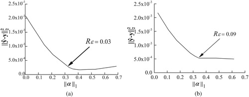
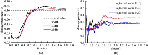
Figure 4 demonstrates the identified results of damage parameters in the two damage cases. Whether in single or multiple damages, the proposed algorithm can accurately identify the location and degree of damage from the VBI vibration signals. The effects of various noise levels are also exhibited in Figure 4 through different gray bars. The identification accuracy decreases slightly with the increase of noise for different damage cases. Simultaneously, the l1-norm regularization process can effectively restrain the fluctuation of the identification results of the undamaged element stiffness, which helps avoid damage misjudgments. Figure 5 displays the convergence process of the identified damage parameters at different noise levels. All identified damage parameters can converge quickly to the real solution. If the identification results of a damage parameter are considered the initial values of the damage parameters, then a secondary identification process can be conducted, and the identification accuracy and convergence rate of the damage parameters can be further improved.

Figure 4. Identification results of local damages. (a) Case 1, (b) Case 2.

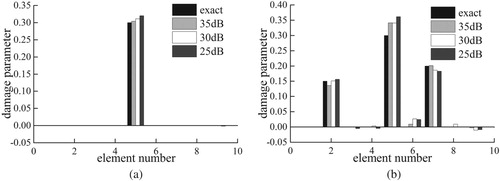
Figure 5. Convergence curve of damage parameters at different noise level. (a) Case 1, (b) Case 2 (noise level is 25 dB).

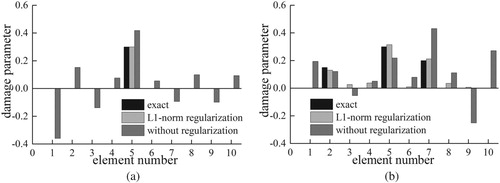
To illustrate the importance of l1-norm regularization, the structural damages estimated by the EKF with and without l1-norm regularization are compared, as presented in Figure 6. Given that the structural responses used in the examples begin when the vehicle enters the bridge and end when the vehicle leaves the bridge, the identification results illustrated in Figure 6 are the results of the moment when the vehicle leaves the bridge. The identification results show that the l1-norm regularization process is essential to correctly assessing the location and extent of structural damage. The results obtained by the EKF without l1-norm regularization cannot indicate the damage. However, introducing the l1-norm regularization, which reflects the prior information of local damages, can effectively compress the solution space and improve the damage identification accuracy.

Figure 6. Local damages identification results with l1-norm regularization or without regularization at the noise level 20 dB. (a) Case 1 (single damage), (b) Case 2 (multiple damages).

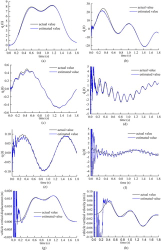
The structural parameters and system state variables are included in the EKF state vector. Therefore, the state of the VBI system can be also estimated in the proposed algorithm. Figure 7 demonstrates the comparison of the identified results of the other variables in the system state vector with actual values at the noise level of 30 dB in Case 2. In Figure 7(a)–(d), the estimated values of the first two bridge modal coordinates and their time derivative are consistent with the actual values after the initial oscillation process, whereas the third-order bridge modal coordinate and the corresponding time derivative oscillate randomly around the true value. Given that the vibration signals of the bridge are dominated by low-frequency components, the third-order modal coordinate and time derivative are smaller than those of the former two modes. Thus, the identified result of the third modal coordinate is easily disturbed by the measurement noise. The small high-order frequency components in the structural response will slightly affect the damage recognition results. The vehicle displacement and its time derivative also depict favourable convergence in Figure 7(g)–(h), although the convergence speed is relatively slower in the vehicle state variables than in the bridge state variables.

Figure 7. Comparison between identified results and actual results of the state variables. (a) the 1st general modal coordinate $q_1\left(t\right)$, (b) time derivative of the 1st general modal coordinate ${\dot{q}}_1\left(t\right)$, (c) the 2nd general modal coordinate $q_2\left(t\right)$, (d) time derivative of the 2nd general modal coordinate ${\dot{q}}_2\left(t\right)$, (e) the 3rd general modal coordinate $q_3\left(t\right)$, (f) time derivative of the 3rd general modal velocity ${\dot{q}}_3\left(t\right)$, (g) vehicle vertical displacement $z\left(t\right)$ (h) vehicle vertical velocity $\dot{z}\left(t\right)$.

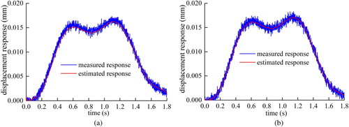
In the EKF recursive process, the estimated displacement response of each measurement point can also be obtained. Figure 8 demonstrates the measured and estimated structural responses at Measurement point 6. The vibration response signals can be accurately tracked under strong noise interference, and the algorithm exhibits a favourable anti-noise performance.

Figure 8. The signal tracing curve at the measurement point 6 at 25 dB noise level. (a) case 1, (b) case 2.

Considering that small structural damages are common, we select four damage degrees of No. 5 element in the single-damage cases to analyze the performance of the damage identification algorithm. Table 2 lists the average relative error of the damage parameters under different noise levels from 100 groups of damage identification results. The average relative error of the damage parameters increases with the decrease in damage degree. Moreover, a large noise indicates that the identification result is easily disturbed by the noise. However, even in the worst case (SNR=20 dB), the average relative error of the small damage element (damage parameter is 5%) is 29.4%, which indicates that the corresponding average absolute error is only 1.5%. Therefore, the algorithm can still guarantee a relatively high identification success rate for small structural damages.

Table 2. The average relative error of damage parameter.

	Noise (SNR)
Damage parameter	20 dB	25 dB	30 dB	35 dB
0.05	29.4%	18.5%	8.66%	4.76%
0.10	15.6%	8.10%	4.10%	3.10%
0.20	7.19%	4.61%	3.47%	2.29%
0.30	5.70%	4.62%	3.28%	2.58%

In addition, to compare the computational efficiency of the different methods in the time domain quantitatively, the traditional time-domain method based on dynamic responses sensitivity analysis in References [16,17] is used. A numerical test is performed on a notebook computer with four Intel(R) Core(TM) i5-7300HQ 2.50 GHz CPU and 8 GB RAM. For the numerical examples in Section 4.1, traditional sensitivity methods typically require 12 iterations to obtain convergence results, and each iteration time is approximately 4.5 s. If all the measured data at all time points are used when the vehicle crosses the bridge, then the algorithm proposed in this work only takes 6.7 s to complete all calculations, and the identification results typically converge after the first two-thirds of the response data are used. Evidently, this method has an improved computational efficiency.

4.1.2. Effect of measurement point number and signal type

The number of measurement points is an important factor that affects the results of damage identification. In the multiple damage case in the previous section, the effect of different measurement point numbers on damage identification is analyzed. The vehicle speed is set to $15\text{m/s}$, and the SNR of the noise-contaminated bridge response is 25 dB. Three kinds of numbers of measurement points and instrumented locations are listed in Table 3. On the basis of the structural displacement or acceleration signals at those measurement points, Figure 9 exhibits the multiple-damage identification results in different cases. The identification accuracy decreases with the number of measurement points, but the structural damages can still be clearly indicated even when the number is reduced to 4. Simultaneously, comparing the results of using the displacement and acceleration signals indicates that the identification accuracy of the two methods is similar.

Figure 9. the identified results of local damages for different measurement number at the noise level 25 dB. (a) Displacement response, (b) acceleration response.

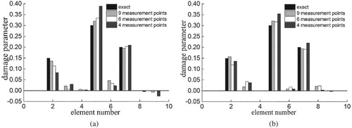
Table 3. Number and location of measurement points.

Number of measurement point	Instrumented locations
9	Node 2,3,4,5,6,7,8,9,10
6	Node 2,3,5,7,9,10
4	Node 3,5,7,9

4.1.3. Effect of different vehicle speeds

Vehicle speed is an important factor that affects the coupling vibration of a vehicle and a bridge. Considering the same structural parameters and damage cases as discussed in Section 4.1.1, the noise-contaminated bridge displacement response at different vehicle speeds is used to identify the structural damage and analyze the effects of vehicle speed. Figure 10 displays the displacement responses of the bridge midpoint at three vehicle speeds. The maximum amplitude of the midpoint response increases nonlinearly with the vehicle speed, and the maximum appears when the vehicle passes the position near the midpoint of the bridge.

Figure 10. The displacement responses in mid-span for different vehicle speed.

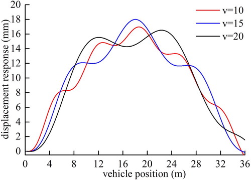
Table 4 lists the relative identification error of the element stiffness at three vehicle speeds in Case 1. For the two measurement noises (25 and 30 dB), the identification errors will increase slightly with the vehicle speed because an increase in vehicle speed will shorten the measurement signal at the same sampling frequency. Thus, using extremely fast vehicle speeds must be avoided in damage detection, and the sampling data of a vibration signal must constantly be sufficient to allow the damage parameters to converge to the exact values. Figure 11 presents the estimated response of Measurement node 5 at the noise level of 25 dB, which nearly coincides completely with the actual response. Therefore, the proposed algorithm can track the actual structural vibration, although the observed signals are contaminated by large noise.

Figure 11. The signal tracing curve of node 5 under 25 dB when $v=40\text{m}/\text{s}$.

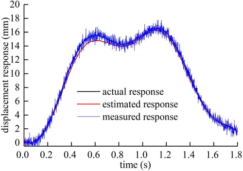
Table 4. The identification error of element stiffness with different vehicle speeds and noise levels.

	30 dB			25 dB
Noise level element	v = 10 m/s	v = 15 m/s	v = 20 m/s	v = 10 m/s	v = 15 m/s	v = 20 m/s
1	0.00%	0.00%	0.00%	0.00%	0.00%	0.00%
2	0.00%	0.00%	0.00%	0.00%	0.00%	0.01%
3	0.00%	0.00%	0.00%	0.00%	0.00%	0.00%
4	0.00%	0.00%	0.00%	0.00%	0.00%	0.00%
5	0.65%	0.94%	1.05%	1.09%	1.34%	1.69%
6	0.00%	0.01%	0.03%	0.02%	0.09%	0.15%
7	0.00%	0.00%	0.00%	0.00%	0.00%	0.00%
8	0.00%	0.00%	0.01%	0.00%	0.02%	0.06%
9	0.00%	0.00%	0.01%	0.01%	0.02%	0.05%
10	0.00%	0.00%	0.00%	0.00%	0.00%	0.00%
Average	0.06%	0.09%	0.13%	0.11%	0.15%	0.20%

4.1.4. Effect of different vehicle weights

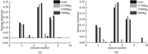
The weight of a vehicle is another important factor that influences the dynamic response of the vehicle–bridge coupling system. Here, three sprung mass $m_2$ values ($5000,15000,\text{and}31700\text{kg}$) are considered, and the other vehicle and bridge parameters are the same as the previous examples. When the vehicle speed is $15\text{m/s}$, Figure 12 illustrates the response of the bridge midpoint for different vehicle weights. The shapes of the response curves are similar, and the displacement amplitude of the bridge is nearly proportional to the vehicle weight. On the basis of the different noise-contaminated displacement responses, the multiple damage identification results demonstrates in Figure 13 show that the proposed algorithm is insensitive to vehicle weight. The maximum relative errors of the damaged and undamaged element stiffness are 6% and 4%, correspondingly.

Figure 12. The displacement responses in mid-span for different vehicle weights.

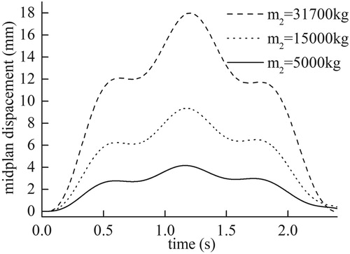
Figure 13. The identified results of local damages for different vehicle weight. (a) Noise level is 30 dB, (b) noise level is 20 dB.

4.2. Example2: continuous beam bridge

In the second numerical experiment, a three-span continuous bridge with moving vehicle excitation is studied to validate the proposed algorithm further. The continuous bridge is evenly divided into 20 Euler–Bernoulli beam elements as depicted in Figure 14, and the details of the assumed geometric and material properties are summarized in Table 5. The parameter values of the vehicle are the same as those in the example presented in Section 4.1, and the moving speed is assumed to be $15\text{m/s}$. The vertical vibration responses of only seven nodes are collected at the sampling frequency of 1000 Hz. Then, Gaussian white noise is added to the vibration signals using Equation (28) to simulate the actual measurement.

Figure 14. Models of the moving vehicle and continuous beam bridge.

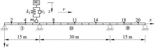
Table 5. Details of the finite element model of the continuous beam bridge.

Parameters	Values
Three-span bridge length	$15\text{m}+30\text{m}+15\text{m}$
Cross section area	$12\times 2.35{\text{m}}^2$
Mass density	$2600\text{kg/}{\text{m}}^2$
Elastic modulus	$34.5\text{GPa}$
Modal damping ratio	3%
Damaged elements and damage parameters	30% at 3rd, 40% at 10th and 20% at 18th
Instrumented locations	Nodes 2, 4, 8, 11, 14, 18 and 20

4.2.1. Damage identification using partial node responses

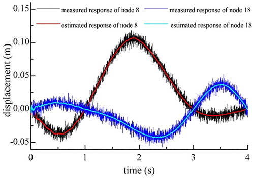
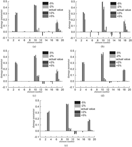
The results exhibited in Figure 15 show that the proposed algorithm successfully captures the exact location and extent of multiple damages using limited measurement nodes. For three noise levels, the maximum relative identification errors of the 3rd, 10th, and 18th damage element stiffness displayed in Figure 15 are 4.9%, 7.1%, and 5.4%, respectively, and the maximum identification errors of the undamaged elements are less than 4.2%. Therefore, the proposed identification method is also applicable to different bridge types. Figure 16 plots the damage parameter convergence curve of the damage elements. Given the inaccuracy of the initial estimation state, the convergence curve oscillates significantly at the beginning, but the damage parameter can quickly converge to the real value with the recursive updating process. Figure 17 illustrates the structural responses estimated by the identification algorithm with the measured and actual structural responses of nodes 8 and 18 at the noise level of 20 dB. The EKF algorithm can suppress the noise well, and the l1-norm regularization process can effectively improve ill-posedness; thus, the estimated response at different measurement nodes is consistent with the actual response.

Figure 15. The identified results of local damages.

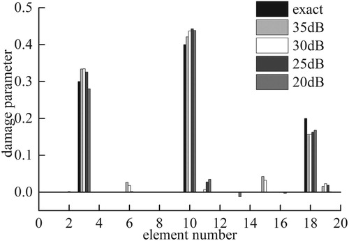
Figure 16. Convergence curve of damage parameter (noise level is 30 dB).

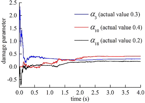
Figure 17. The signal tracing curve at different measure point (20 dB).

The effect of vehicle speed and weight on the identification results is also studied in this example. Tables 6 and 7 list the relative identification errors of the damage parameters for three vehicle speeds and three vehicle weights. Similar conclusions presented in Section 4.1 can be obtained. The proposed algorithm can effectively identify the local damages and is insensitive to vehicle speed and weight.

Table 6. Identification errors of damage parameter for different vehicle speeds.

	v = 15 m/s			v = 30 m/s			v = 40 m/s
	30 dB	25 dB	20 dB	30 dB	25 dB	20 dB	30 dB	25 dB	20 dB
${\alpha }_3$	3.25%	0.73%	1.22%	1.45%	1.41%	2.14%	2.59%	6.16%	8.56%
${\alpha }_{10}$	1.86%	2.23%	5.71%	2.79%	4.11%	5.45%	7.94%	10.12%	14.30%
${\alpha }_{18}$	7.36%	8.55%	6.36%	8.32%	8.82%	6.78%	9.87%	8.12%	5.03%

Table 7. Identification errors of damage parameter for different vehicle weights.

	m2 = 5000 kg			m2 = 15,000 kg			m2 = 31,700 kg
	30 dB	25 dB	20 dB	30 dB	25 dB	20 dB	30 dB	25 dB	20 dB
${\alpha }_3$	2.52%	2.15%	0.66%	5.29%	4.61%	3.09%	3.63%	1.16%	2.27%
${\alpha }_{10}$	7.83%	7.52%	3.44%	1.74%	1.50%	2.24%	3.01%	4.46%	2.33%
${\alpha }_{18}$	10.07%	10.24%	12.39%	7.29%	7.56%	8.22%	6.96%	6.98%	8.15%

4.2.2. Effect of modelling errors

In the previous examples, an ideal assumption is that other structural parameters are perfectly known when the changes in element stiffness are identified. Typically, only an imperfect bridge and vehicle model can be used in a real inverse analysis. To analyze the effect of modelling errors, the typical model parameters, including unsprung mass $m_1$, sprung mass $m_2$, spring stiffness $k_1$, and damping coefficient $c_1$, of a vehicle and the modal damping ratio of the bridge are selected, and four deviation levels from the true values, that is, $\pm 2\mathrm{\%}$ and $\pm 5\mathrm{\%}$, are considered. The results depicted in Figure 18 shows that the deviation in the sprung mass value has the most significant influence on the identification results among the five model parameters. An increase in the inaccuracy of model parameter values will gradually reduce the accuracy of the damage identification results, but the maximum relative identification error of the damage element stiffness remains less than 15% even in the deviation level of $\pm 5\mathrm{\%}$. The main damages can be clearly indicated because the interference of noise on the identification results of an undamaged element is suppressed well. Therefore, the proposed algorithm also shows robustness to the modelling error.

Figure 18. The identification results when imperfect model is considered (SNR is 20 dB). (a) unsprung mass $m_1$, (b) sprung mass $m_2$, (c) spring stiffness $k_1$, (d) damping coefficient $c_1$, (e) modal damping ratio of bridge.

5. Damage identification of the bridge with road roughness

When road roughness is considered in the VBI system, the damage identification problem of the bridge structure is significantly different from the damage identification problem discussed in Section 3. In Section 3, the moving vehicle is the only excitation source, and thus the load is known for the identification problem. However, damage detection problem changes to a system parameter identification problem with an unknown load when the random and unknown road roughness is considered. The synchronous identification of unknown structural parameters and loads will increase the identification difficulty and computational complexity considerably. Therefore, in accordance with the method provided in Section 3, a simplified method based on the VBI model with a smooth road is proposed to identify the structural damage of the bridge with road roughness.

5.1. Effect of road roughness and simplified method for structural damage identification

When road roughness is considered, the VBI system motion equation can still be expressed as (30) $\mathit{M}\ddot{\mathit{q}}+\mathit{C}\dot{\mathit{q}}+\mathit{K}\mathit{q}=\mathit{F},$(30) where $\mathit{M}$, $\mathit{C}$, and $\mathit{K}$ are the same with those in Equation (4), but the load item must be modified to include the effects of road roughness. (31) $\mathit{F}={\mathit{F}}_{\mathit{v}}+{\mathit{F}}_{\mathit{r}},$(31) where $r^{\mathrm{\prime }}=\left(\text{d}r\text{/d}x\right)$, and (32a) ${\mathit{F}}_{\mathit{v}}=\left(m_1+m_2\right)g{\left[\begin{array}{cccc}{\phi }_1& \cdots & {\phi }_n& 0\end{array}\right]}^T,$(32a) (32b) ${\mathit{F}}_{\mathit{r}}=-\left(cv{r}^{\mathrm{\prime }}+kr\right){\left[\begin{array}{cccc}{\phi }_1& \cdots & {\phi }_n& 1\end{array}\right]}^T.$(32b) where ${\mathit{F}}_{\mathit{v}}$ has the same form as $\mathit{F}$ in Equation (4d) and is unrelated to road roughness.

Given that Equation (30) is a linear differential equation with time-varying coefficients, the solution of the equation satisfies the superposition principle, so the solution can be divided into two parts. (33) $\mathit{q}={\mathit{q}}_v+{\mathit{q}}_r,$(33) where ${\mathit{q}}_v$ and ${\mathit{q}}_r$ are associated with the moving vehicle and road roughness, correspondingly. Therefore, the vibration response of the bridge under a moving vehicle is also divided into two parts when road roughness is considered. (34) $\mathit{u}\left(x,t\right)=\sum _{i=1}^N{p}_i\left(t\right){\phi }_i\left(x\right)=\mathit{\Phi }\cdot \mathit{T}\cdot \left({\mathit{q}}_v+{\mathit{q}}_r\right)=\mathit{\Phi }\cdot \mathit{T}\cdot {\mathit{q}}_v+\mathit{\Phi }\cdot \mathit{T}\cdot {\mathit{q}}_r={\mathit{u}}_v+{\mathit{u}}_r$(34) where $\mathit{T}=\left[\begin{array}{cc}\mathit{I}& 0\end{array}\right]$ is the transfer matrix. ${\mathit{u}}_v$ and ${\mathit{u}}_{\mathit{r}}$ are the bridge displacements caused by the moving vehicle and road roughness, respectively. In comparison with the vehicle–bridge coupled vibration response without considering road roughness, only response$\text{ }{u}_r$ is added to the bridge vibration response after considering the road roughness.

When the identification algorithm based on the VBI model with a smooth road is used to detect the structural damage of the bridge with road roughness, the state equations of the VBI system identification remain unchanged. (35) $\dot{\mathit{\theta }}\left(t\right)=\mathit{f}\left(\mathit{\theta },t\right)+\mathit{W}$(35) However, the response values associated with road roughness must be supplemented in the observation equation. (36) $\mathit{y}\left(\mathit{x},t\right)=\mathit{h}\left(\mathit{\theta }\left(t\right),\mathit{x},t\right)+{\mathit{u}}_r+\mathit{V}$(36) where ${\mathit{u}}_r$ is an unknown random variable that is related to roughness, bridge structure, and vehicle speed. The unknown response in the observation equation will hinder the recursive process of the KF. In this work, we do not directly identify the unknown response ${\mathit{u}}_r$, but rather use a simplified approach on the basis of the favourable robustness of the KF algorithm. Under equal noise mean and variance conditions, the random observation noises with non-Gaussian distributions (such as uniform, Gamma, and Rayleigh distributions) and Gaussian distribution have a similar effect on the error performance of the KF [42]; thus, non-Gaussian noise can be approximated as Gaussian noise with the same mean and variance in engineering applications when the statistical differences between non-Gaussian and Gaussian variables are small. Therefore, we consider the random response ${\mathit{u}}_r$ caused by road roughness and the actual noise $\mathit{V}$ as the total observation noise, $\tilde{\mathit{V}}={\mathit{u}}_{\mathit{r}}+\mathit{V}$. By using the robustness of the EKF algorithm, the structural damages under non-Gaussian measurement noise are identified through a direct use of the EKF method in Section 3.

5.2. Bridge response caused by road roughness

Road surface [10] is typically assumed to be a stationary Gaussian random process and can be generated through an inverse Fourier transformation based on spectral density functions as (37) $r\left(x\right)=\sum _{k=1}^N\sqrt{2G_d\left(n_k\right)\mathrm{\Delta }n}\cos \left(2\pi n_{k}x-{\theta }_k\right),$(37) where $n_k$ is the spatial frequency; $\mathrm{\Delta }n=\left(n_u-n_l\right)\text{/}N$, where $n_u$ and $n_l$ are the upper and lower cut-off frequencies, correspondingly; ${\theta }_k$ is the random phase angle that is uniformly distributed from 0 to $2\pi$; the power spectral density function $G_d\left(n_k\right)$ is selected in accordance with ISO-8068 [43] as (38) $G_q\left(n\right)=G_q\left(n_0\right){\left(\frac{n}{n_0}\right)}^{-2},$(38) where $n$ is the spatial frequency, $n_0$ is the reference spatial frequency, and $G_q\left(n_0\right)$ 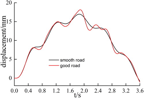is the roughness coefficient whose value is selected depending on the road condition. The bridge surface condition [44] can be classified as good, average, and poor in accordance with the ISO specification Classes A–C. Most of the bridge surfaces are categorized in good to average condition. For the simply supported bridge model in Section 4.1, Figure 19 demonstrates a typical road surface profile that belongs to the good road surface condition, and Figure 20 exhibits the corresponding vibration response ($\mathit{u}$) at the mid node of the bridge when the vehicle speed is 10 m/s. In comparison with the vibration response ${\mathit{u}}_v$ of the bridge with a smooth surface, random road roughness may cause response $\mathit{u}$ to fluctuate near$\text{ }{\mathit{u}}_v$, and response difference ${\mathit{u}}_r$ is a random signal that consists mainly of several low-frequency components.

Figure 19. Typical roughness of good road surface condition.

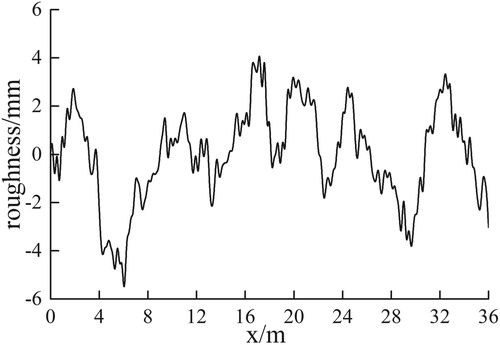
Figure 20. Vibration response of the bridge midpoint under different road surface.

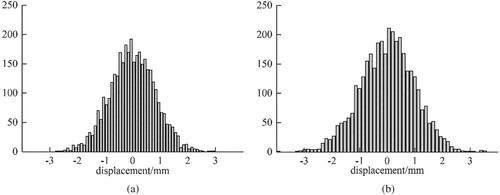
Initial observation noise $\mathit{V}$ and total observation noise $\tilde{\mathit{V}}$ are displayed in Figure 21. In this figure, the total observation noise $\tilde{\mathit{V}}$ has more low-frequency components than Gaussian observation noise $\mathit{V}$. However, in accordance with the probability density function presented in Figure 22, the total observation noise can be considered similar to Gaussian noise. Therefore, the damage identification problem in Equations (35) and (36) can be analyzed directly by the proposed EKF algorithm. Notably, the response ${\mathit{u}}_r$ related to road roughness will increase for poor road condition, and then the increase in the difference between observation noise $\tilde{\mathit{V}}$ and standard Gaussian noise may lead to a decrease in identification accuracy. Therefore, the simplified damage identification method proposed in this work is suitable for good road conditions.

Figure 21. Measurement noise. (a) initial measurement noise, (b) total measurement noise

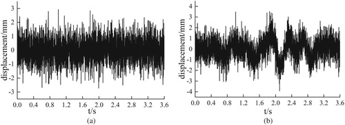
Figure 22. Probability density function of observation noise. (a) initial observation noise $\mathit{V}$ (b) total observation noise $\tilde{\mathit{V}}$.

5.3. Damage identification results of the bridge with road roughness

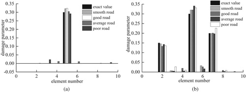
A simply support bridge example presented in Section 4.1 under three levels of road surface conditions, namely, good, average, and poor, are studied according to the reference [44]. The typical damage identification results under a moving vehicle with 10 m/s velocity are illustrated in Figure 23. The location and extent of structural damage can still be identified accurately when the road roughness of the bridge is considered.

Figure 23. Damage identification results of bridge under different road surface condition (noise level is 25 dB and vehicle velocity is 10 m/s). (a) single damage. (b) multiple damages.

Considering the randomness of the road surface roughness and the observation noise, the damage identification result must be random. Thus, the identification success rate based on the statistical analysis of multiple simulation results is used to illustrate the effectiveness of the algorithm. ${\alpha }_i^u$ and ${\alpha }_i^d$ are defined for the identification results of damage parameters in undamaged and damaged elements, and ${\alpha }_i^{\ast }$ is set as a real damage parameter. A successful identification is defined as $|{\alpha }_i^u-{\alpha }_i^{\ast }|<0.05$ and $|{\alpha }_i^d-{\alpha }_i^{\ast }|<0.1$ for a group of random observation noise and road roughness, and then the success rate is the percentage of success identification in all test groups (the number of test groups in this work is 100).

Table 8 lists the success rates of damage identification in different damage cases, road conditions, noise levels, and signal types when the vehicle velocity is 10 m/s. The results show that a slight road roughness indicates a high success rate of damage identification. In the simply supported beam example, the success rate of damage identification based on displacement signals can exceed 80% for the bridge with a good surface condition in different damage cases when the SNR is greater than 30 dB. In addition, the success rate is higher in the single damage case than in the complex multi-damage case. For the single damage case, the success rate of the bridge with an average road roughness can still reach 100% even at the noise level of 25 dB.

Table 8. Successful identification rate under different road surface ($v=10\text{m/s}$).

		Displacement signal			Acceleration signal
Case	Road	25 dB	30 dB	35 dB	25 dB	30 dB	35 dB
Single damage	smooth	100%	100%	100%	100%	100%	100%
	good	100%	100%	100%	79%	95%	98%
	average	100%	100%	100%	73%	91%	96%
	poor	85%	100%	100%	68%	86%	90%
Multiple damages	smooth	76%	97%	100%	100%	100%	100%
	good	71%	83%	100%	58%	79%	83%
	average	60%	67%	100%	46%	58%	75%
	poor	33%	48%	92%	22%	53%	71%

Table 8 also summarizes the damage identification results of the proposed algorithm on the basis of the different measurement signals. For a smooth road, the damage identification algorithm can obtain ideal results, regardless of the acceleration or displacement signals. When road roughness is considered, the difference in identification results caused by various signals becomes significant. The influence of roughness is greater on the acceleration responses than on the structural displacement, especially in high-frequency components. Therefore, the total measurement noise (including the random response caused by road roughness and the actual noise) in the simplified method based on acceleration signals will deviate further from the assumption of Gaussian noise. In accordance with the success rate of damage identification, the algorithm based on displacement signal is better than the algorithm based on acceleration signals.

In Section 4, the numerical cases show that vehicle speed is insensitive to the bridge damage identification for the smooth road surface, but the effect of vehicle speed will become increasingly significant when the roughness of a bridge deck is considered. Table 8 lists the identification success rates at different vehicle speeds for the single damage case. The proportion of vibration components ${\mathit{u}}_{\mathit{r}}$ caused by road roughness in the total noise $\tilde{\mathit{V}}$ will gradually increase with the vehicle speed; therefore, the success rate of the damage identification results summarized in Table 9 will decrease with the increase in vehicle speed.

Table 9. Successful identification rate under different vehicle velocity.

		v (m/s)
SNR	Road	10	15	20	25
30 dB	smooth	100%	100%	100%	100%
	good	100%	100%	100%	100%
	average	100%	100%	100%	100%
	poor	100%	99%	99%	98%
25 dB	smooth	100%	100%	100%	100%
	good	100%	100%	100%	97%
	average	100%	96%	92%	86%
	poor	85%	73%	65%	63%

According to the abovementioned analysis, the damage identification method based on the vehicle–bridge coupled vibration proposed in this work can be applied to the case where the random and unknown road roughness is considered and has favourable damage identification ability under good road conditions.

6. Conclusions

Existing damage detection methods for bridges under moving vehicle loads require a simultaneous use of entire vibration responses and response sensitivity to construct and solve high-dimensional algebraic equations. As a real-time detection algorithm with a recursive form, a new damage detection method for bridge structures under moving vehicular loads is proposed on the basis of the EKF and l1-norm regularization. The structural damage parameters and state variables of a bridge are updated constantly to obtain the optimal estimate in the recursive process of the EKF in accordance with the vehicle-induced responses of the damaged bridge. Using the sparsity of the structural damage parameter distribution, the l1-norm regularization process is introduced into the EKF framework through the PM technique to improve the ill-posedness of the inverse problem. Numerical studies on a simple-supported and continuous beam bridge deck subject to a four-parameter moving vehicle are studied separately to validate the proposed algorithm. Given that the l1-norm regularization clearly improves the ill-posedness, the EKF algorithm with l1-norm regularization can identify all the structural damages and state vectors accurately even in the case of a 25 dB noise. Furthermore, using the favourable robustness of the EKF, the proposed algorithm can be directly applied to identify the structural damages of the bridge with road roughness after increasing the measurement noise. Through an impact analysis of vehicle speed, vehicle weight, and bridge type, the simplified approach can be used as a useful and reliable tool for the condition assessment of bridge structures, especially for bridges with smooth and good road conditions. In the future, the proposed algorithm can also be combined with substructures, element grouping, and other techniques to evaluate the health status of additional complex structures.

Acknowledgments

This research is partially funded by the National Natural Science Foundation of China (No. 51268045 and 51469016). The authors gratefully acknowledge these supports.

Disclosure statement

No potential conflict of interest was reported by the authors.

ORCID

Chun Zhang http://orcid.org/0000-0001-6779-8609

Additional information

Funding

This research is partially funded by the National Natural Science Foundation of China [grant number 51268045] and [grant number 51469016].

Appendix

To obtain$\frac{\mathrm{\partial }\mathit{L}}{\mathrm{\partial }\mathit{\alpha }}$, $\frac{\mathrm{\partial }\mathit{B}}{\mathrm{\partial }\mathit{\alpha }}$, and $\frac{\mathrm{\partial }{\mathit{F}}_f}{\mathrm{\partial }\mathit{\alpha }}$ in Section 3.1, we first calculate $\frac{\mathrm{\partial }\mathit{L}}{\mathrm{\partial }{\alpha }_i}$, $\frac{\mathrm{\partial }\mathit{B}}{\mathrm{\partial }{\alpha }_i}$, and $\frac{\mathrm{\partial }{\mathit{F}}_f}{\mathrm{\partial }{\alpha }_i}$, where $\mathit{L}={\mathit{M}}^{-1}\mathit{K}$, and $\mathit{B}={\mathit{M}}^{-1}\mathit{C}$. The sensitivity calculation involves the derivation of matrix ${\mathit{M}}^{-1}$. Given that matrix $\mathit{M}$ is time-varying, directly calculating ${\mathit{M}}^{-1}$ and $\frac{\mathrm{\partial }{\mathit{M}}^{-1}}{\mathrm{\partial }{\alpha }_i}$ in each recursive step requires a high computational cost. Therefore, this work uses the Neumann series expansion method to simplify the calculation of ${\mathit{M}}^{-1}$. The mass matrix of the vehicle–bridge coupling system can be expressed as $\mathit{M}={\mathit{M}}_0+\mathrm{\Delta }\mathit{M},$ where $\begin{array}{rlr}{\mathit{M}}_0& =\left[\begin{array}{ccccc}1& 0& \cdots & 0& 0\\ 0& 1& \cdots & 0& 0\\ ⋮& ⋮& \cdots & ⋮& ⋮\\ 0& 0& \cdots & 1& 0\\ 0& 0& \cdots & 0& m_2\end{array}\right],& \mathrm{\Delta }\mathit{M}=m_1\left[\begin{array}{ccccc}{\Phi }_{11}& {\Phi }_{12}& \cdots & {\Phi }_{1N}& 0\\ {\Phi }_{21}& {\Phi }_{22}& \cdots & {\Phi }_{2N}& 0\\ ⋮& ⋮& \cdots & ⋮& ⋮\\ {\Phi }_{N1}& {\Phi }_{N2}& \cdots & {\Phi }_{NN}& 0\\ 0& 0& \cdots & 0& 0\end{array}\right]\\ & =m_1\left[\begin{array}{cc}{\mathit{\phi }}^T\mathit{\phi }& 0\\ 0& 0\end{array}\right].\end{array}$ where $\mathit{\phi }={\left.\left[\begin{array}{ccc}{\mathit{\phi }}_1& \cdots & {\mathit{\phi }}_N\end{array}\right]\right|}_{x=vt}$, and ${\mathit{\phi }}_i$ is the ith mass-normalized mode shape. In accordance with the Neumann series extension formula, the inverse of the generalized mass matrix can be written as ${\mathit{M}}^{-1}=({\mathit{M}}_0+\mathrm{\Delta }\mathit{M}{)}^{-1}=\left(\mathit{I}-\mathit{P}+{\mathit{P}}^2-\cdots \right){\mathit{M}}_0^{-1}$ where $\mathit{P}={\mathit{M}}_0^{-1}\mathrm{\Delta }\mathit{M}$. If only the first two terms are considered, then ${\mathit{M}}^{-1}$ can be written as ${\mathit{M}}^{-1}=\left(\mathit{I}-{\mathit{M}}_0^{-1}\mathrm{\Delta }\mathit{M}\right){\mathit{M}}_0^{-1},$ and the corresponding derivation can be obtained as $\begin{array}{ccc}\frac{\mathrm{\partial }{\mathit{M}}_0}{\mathrm{\partial }{\alpha }_i}=0,& \frac{\mathrm{\partial \Delta }\mathit{M}}{\mathrm{\partial }{\alpha }_i}=m_1\mathit{\Psi },& \mathit{\Psi }=\left[\begin{array}{cc}{\left(\frac{\mathrm{\partial }\phi }{\mathrm{\partial }{\alpha }_i}\right)}^T\cdot \mathit{\phi }+{\mathit{\phi }}^T\cdot \frac{\mathrm{\partial }\mathit{\phi }}{\mathrm{\partial }{\alpha }_i}& \mathbf{0}\\ \mathbf{0}& 0\end{array}\right]\end{array}.$ Similarly, the stiffness and damping matrices of the vehicle–bridge coupling system can be expressed as $\mathit{K}={\mathit{K}}_0+\mathrm{\Delta }\mathit{K},$ $\mathit{C}={\mathit{C}}_0+\mathrm{\Delta }\mathit{C},$ where $\begin{array}{ccc}{\mathit{K}}_0=\left[\begin{array}{cc}{\mathit{\Lambda }}_K& -k_1{\mathit{\phi }}^T\\ -k_1\mathit{\phi }& k_1\end{array}\right],& \mathrm{\Delta }\mathit{K}=k_1\left[\begin{array}{cc}{\mathit{\phi }}^T\mathit{\phi }& \mathbf{0}\\ \mathbf{0}& 0\end{array}\right],& {\mathit{\Lambda }}_K=\text{diag}\left(\left\{\begin{array}{ccc}{\omega }_1^2& \cdots & {\omega }_N^2\end{array}\right\}\right)\end{array},$ $\begin{array}{ccc}{\mathit{C}}_0=\left[\begin{array}{cc}{\mathit{\Lambda }}_C& -c_1{\mathit{\phi }}^T\\ -c_1\mathit{\phi }& c_1\end{array}\right],& \mathrm{\Delta }\mathit{C}=c_1\left[\begin{array}{cc}{\mathit{\phi }}^T\mathit{\phi }& \mathbf{0}\\ \mathbf{0}& 0\end{array}\right],& {\mathit{\Lambda }}_C=\text{diag}\left(\left\{\begin{array}{ccc}2{\xi }_1{\omega }_1& \cdots & 2{\xi }_N{\omega }_N\end{array}\right\}\right)\end{array}.$ and the corresponding partial derivatives are $\begin{array}{cc}\frac{\mathrm{\partial }{\mathit{K}}_0}{\mathrm{\partial }{\alpha }_i}=\left[\begin{array}{cc}\frac{\mathrm{\partial }{\mathit{\Lambda }}_K}{\mathrm{\partial }{\alpha }_i}& -k_1\frac{\mathrm{\partial }{\mathit{\phi }}^T}{\mathrm{\partial }{\alpha }_i}\\ -k_1\frac{\mathrm{\partial }\mathit{\phi }}{\mathrm{\partial }{\alpha }_i}& 0\end{array}\right]={\mathit{K}}_{0\alpha },& \frac{\mathrm{\partial \Delta }\mathit{K}}{\mathrm{\partial }{\alpha }_i}=k_1\left[\begin{array}{cc}\frac{\mathrm{\partial }{\phi }^T}{\mathrm{\partial }{\alpha }_i}\cdot \mathit{\phi }+{\mathit{\phi }}^T\cdot \frac{\mathrm{\partial }\mathit{\phi }}{\mathrm{\partial }{\alpha }_i}& 0\\ \mathbf{0}& 0\end{array}\right]=k_1\mathit{\Psi }\end{array},$ $\begin{array}{cc}\frac{\mathrm{\partial }{\mathit{C}}_0}{\mathrm{\partial }{\alpha }_i}=\left[\begin{array}{cc}\frac{\mathrm{\partial }{\mathit{\Lambda }}_C}{\mathrm{\partial }{\alpha }_i}& -c_1\frac{\mathrm{\partial }{\mathit{\phi }}^T}{\mathrm{\partial }{\alpha }_i}\\ -c_1\frac{\mathrm{\partial }\mathit{\phi }}{\mathrm{\partial }{\alpha }_i}& 0\end{array}\right]={\mathit{C}}_{0\alpha },& \frac{\mathrm{\partial \Delta }\mathit{C}}{\mathrm{\partial }{\alpha }_i}=c_1\left[\begin{array}{cc}\frac{\mathrm{\partial }{\phi }^T}{\mathrm{\partial }{\alpha }_i}\cdot \mathit{\phi }+{\mathit{\phi }}^T\cdot \frac{\mathrm{\partial }\mathit{\phi }}{\mathrm{\partial }{\alpha }_i}& 0\\ \mathbf{0}& 0\end{array}\right]=c_1\mathit{\Psi }\end{array}.$ Therefore, $\frac{\mathrm{\partial }\mathit{L}}{\mathrm{\partial }{\alpha }_i}$,$\text{ }\frac{\mathrm{\partial }\mathit{B}}{\mathrm{\partial }{\alpha }_i}$ and $\text{ }\frac{\mathrm{\partial }{\mathit{F}}_f}{\mathrm{\partial }{\alpha }_i}$ can be calculated as $\begin{array}{rl}\frac{\mathrm{\partial }\mathit{L}}{\mathrm{\partial }{\alpha }_i}& =\frac{\mathrm{\partial }\left({\mathit{M}}^{-1}\mathit{K}\right)}{\mathrm{\partial }{\alpha }_i}=\frac{\mathrm{\partial }{\mathit{M}}^{-1}}{\mathrm{\partial }{\alpha }_i}\mathit{K}+{\mathit{M}}^{-1}\frac{\mathrm{\partial }\mathit{K}}{\mathrm{\partial }{\alpha }_i}=-m_1{\mathit{M}}_0^{-1}{\mathit{\Psi }\mathit{M}}_0^{-1}\mathit{K}\\ & +\left(\mathit{I}-{\mathit{M}}_0^{-1}\mathrm{\Delta }\mathit{M}\right){\mathit{M}}_0^{-1}\left({\mathit{K}}_{0\alpha }+k_1\mathit{\Psi }\right),\end{array}$ $\begin{array}{rl}\frac{\mathrm{\partial }\mathit{B}}{\mathrm{\partial }{\alpha }_i}& =\frac{\mathrm{\partial }\left({\mathit{M}}^{-1}\mathit{C}\right)}{\mathrm{\partial }{\alpha }_i}=\frac{\mathrm{\partial }{\mathit{M}}^{-1}}{\mathrm{\partial }{\alpha }_i}\mathit{C}+{\mathit{M}}^{-1}\frac{\mathrm{\partial }\mathit{C}}{\mathrm{\partial }{\alpha }_i}=-m_1{\mathit{M}}_0^{-1}{\mathit{\Psi }\mathit{M}}_0^{-1}\mathit{C}\\ & +\left(\mathit{I}-{\mathit{M}}_0^{-1}\mathrm{\Delta }\mathit{M}\right){\mathit{M}}_0^{-1}\left({\mathit{C}}_{0\alpha }+c_1\mathit{\Psi }\right),\end{array}$ $\frac{\mathrm{\partial }{\mathit{F}}_f}{\mathrm{\partial }{\alpha }_i}=\frac{\mathrm{\partial }\left({\mathit{M}}^{-1}\mathit{F}\right)}{\mathrm{\partial }{\alpha }_i}=\frac{\mathrm{\partial }{\mathit{M}}^{-1}}{\mathrm{\partial }{\alpha }_i}\mathit{F}+{\mathit{M}}^{-1}\frac{\mathrm{\partial }\mathit{F}}{\mathrm{\partial }{\alpha }_i}=-m_1{\mathit{M}}_0^{-1}{\mathit{\Psi }\mathit{M}}_0^{-1}\mathit{F}+\left(\mathit{I}-{\mathit{M}}_0^{-1}\mathrm{\Delta }\mathit{M}\right){\mathit{M}}_0^{-1}{\mathit{F}}_{\alpha },$

where ${\mathit{F}}_{\alpha }=\left(m_1+m_2\right)g{\left[\begin{array}{cc}\left(\mathrm{\partial }\mathit{\phi }/\mathrm{\partial }{\alpha }_i\right)& 0\end{array}\right]}^T$.

References

- Doebling SW, Farrar CR, Prime MB. A summary review of vibration-based damage identification methods. Shock Vibr Digest. 1998;30(2):91–105.
- Carden EP. Vibration based condition monitoring: a review. Struct Health Monit. 2004;3(4):355–377.
- Brownjohn JMW. Structural health monitoring of civil infrastructure. Philos Trans R Soc A: Math Phys Eng Sci. 2007;365(1851):589–622.
- Fan W, Qiao P. Vibration-based damage identification methods: a review and comparative study. Struct Health Monit. 2010;9(3):83–111.
- Kim J, Lynch JP, Lee JJ, et al. Truck-based mobile wireless sensor networks for the experimental observation of vehicle-bridge interaction. Smart Mater Struct. 2011;20(6):1645–1648.
- Zhu XQ, Law SS. Recent developments in inverse problems of vehicle–bridge interaction dynamics. J Civil Struct Health Monit. 2016;6(1):107–128.
- Yang YB, Yang JP. State-of-the-art review on modal identification and damage detection of bridges by moving test vehicles. Int J Struct Stab Dyn. 2017;6:1850025.
- Zhu XQ, Law SS. Wavelet-based crack identification of bridge beam from operational deflection time history. Int J Solids Struct. 2006;43(43):2299–2317.
- Hester D, González A. A wavelet-based damage detection algorithm based on bridge acceleration response to a vehicle. Mech Syst Signal Process. 2012;28(2):145–166.
- Sun Z, Nagayama T, Su D, et al. A damage detection algorithm utilizing dynamic displacement of bridge under moving vehicle. Shock Vib. 2016;6:1–9.
- Li J, Law SS. Damage identification of a target substructure with moving load excitation. Mech Syst Signal Process. 2012;30(7):78–90.
- He X, Kawatani M, Hayashikawa T, et al. A bridge damage detection approach using Train-bridge interaction analysis and GA optimization. Procedia Eng. 2011;14(2259):769–776.
- Zhan JW, Xia H, Chen SY, et al. Structural damage identification for railway bridges based on train-induced bridge responses and sensitivity analysis. J Sound Vib. 2011;330(4):757–770.
- Roveri N, Carcaterra A. Damage detection in structures under traveling loads by Hilbert–huang transform. Mech Syst Signal Process. 2012;28:128–144.
- Meredith J, Gonzalez A, Hester D. Empirical mode decomposition of the acceleration response of a prismatic beam subject to a moving load to identify multiple damage locations. Shock Vib. 2012;19(5):845–856.
- Lu ZR, Liu JK. Identification of both structural damages in bridge deck and vehicular parameters using measured dynamic responses. Comput Struct. 2011;89(13):1397–1405.
- Zhang X, Sun G, Sun Y, et al. Simultaneous identification of vehicular parameters and structural damages in bridge. Wuhan Univ J Nat Sci. 2018;23(1):84–92.
- Li J, Law SS, Hao H. Improved damage identification in bridge structures subject to moving loads: numerical and experimental studies. Int J Mech Sci. 2013;74(3):99–111.
- Feng D, Feng MQ, et al. Model updating of railway bridge using in situ dynamic displacement measurement under trainloads. J Bridge Eng. 2015;20(12):04015019.
- Liu X, Escamilla-Ambrosio PJ, Lieven NAJ. Extended Kalman filtering for the detection of damage in linear mechanical structures. J Sound Vib. 2009;325(4-5):1023–1046.
- Ding Y, Zhao BY, Wu B, et al. A condition assessment method for time-variant structures with incomplete measurements. Mech Syst Signal Process. 2015;58:228–244.
- Lai Z, Lei Y, Zhu S, et al. Moving-window extended Kalman filter for structural damage detection with unknown process and measurement noises. Measurement. 2016;88:428–440.
- Liu L, Su Y, Zhu J, et al. Data fusion based EKF-UI for real-time simultaneous identification of structural systems and unknown external inputs. Measurement. 2016;88:456–467.
- Yang JN, Lin S, Huang H, et al. An adaptive extended Kalman filter for structural damage identification. Struct Control Health Monit. 2006;13(4):849–867.
- Yang JN, Pan S, Huang H. An adaptive extended Kalman filter for structural damage identifications II: unknown inputs. Struct Control Health Monit. 2007;14(3):497–521.
- Zhou Q, Liu Y, Wang X, et al. Structural damage detection technique with limited input and output measurement signals. Mech Syst Signal Process. 2012;26(5):229–243.
- Lei Y, Wu Y, Li T. Identification of non-linear structural parameters under limited input and output measurements. Int J Non Linear Mech. 2012;47(10):1141–1146.
- Weber B, Paultre P, Proulx J. Consistent regularization of nonlinear model updating for damage identification. Mech Syst Signal Process. 2009;23(6):1965–1985.
- Rucevskis S, Sumbatyan MA, Akishin P, et al. Tikhonov’s regularization approach in mode shape curvature analysis applied to damage detection. Mech Res Commun. 2015;65:9–16.
- Zhang C, Huang J-Z, Song G-Q, et al. Detection of structural damage via free vibration responses by extended Kalman filter with Tikhonov regularization scheme. Struct Monit Maint, Int J. 2016;3(2):115–127.
- Park HW, Man WP, Ahn BK, et al. 1-Norm-based regularization scheme for system identification of structures with discontinuous system parameters. Int J Numer Methods Eng. 2007;69(3):504–523.
- Zhang CD, Xu YL. Comparative studies on damage identification with Tikhonov regularization and sparse regularization. Struct Control Health Monit. 2016;23(3):560–579.
- Zhou S, Bao Y, Li H, et al. Structural damage identification based on substructure sensitivity and l1sparse regularization. //SPIE Smart Structures and Materials+ Nondestructive Evaluation and Health Monitoring. International Society for Optics and Photonics, 2013; 8692:86923N1-86923N8.
- Mascarenas D, Cattaneo A, Theiler J, et al. Compressed sensing techniques for detecting damage in structures. Struct Health Monit. 2013;12(4):325–338.
- Yang Y, Nagarajaiah S. Output-only modal identification by compressed sensing: Non-uniform low-rate random sampling. Mech Syst Signal Process. 2015;56-57:15–34.
- Grewal MS, Andrews AP. Kalman filtering: theory and practice using MATLAB. 2nd ed. New York: John Wiley and Sons, Inc.; 2001.
- James G M, Peter R, Lv J. DASSO: connections between the Dantzig selector and lasso. J R Stat Soc. 2009;71(1):127–142.
- Carmi A, Gurfil P, Kanevsky D. Methods for sparse signal Recovery using Kalman filtering with embedded pseudo-measurement norms and quasi-norms. IEEE Trans Signal Process. 2010;58(4):2405–2409.
- Lawson CL, Hanson RJ. Solving least squares problems. Englewood Cliffs, NJ: Prentice-Hall; 1974.
- Feng D, Sun H, Feng MQ. Simultaneous identification of bridge structural parameters and vehicle loads. Comput Struct. 2015;157:76–88.
- Karoumi R. Response of cable-stayed and suspension bridges to moving vehicles: analysis methods and practical modeling techniques. Stockholm: KTH Royal Institute of Technology; 1998.
- Jinguang C, Lili MA. Error performance analysis of Kalman filtering algorithm for Non-Gaussian system. Electron Optics Control. 2010;17(9):30–33. (in Chinese).
- International Organization for Standardization (ISO). Mechanical vibration-road surface profiles-reporting of measured data. ISO 8068: 1995 (E), ISO.Geneva; 1995.
- Honda H, Kajikawa Y, Kobori T. Spectra of road surface roughness on bridges. J Struct Div. 1982;108(9):1956–1966.
Appendix
To obtain,
, and
in Section 3.1, we first calculate
,
, where
. The sensitivity calculation involves the derivation of matrix
. Given that matrix
is time-varying, directly calculating
and
in each recursive step requires a high computational cost. Therefore, this work uses the Neumann series expansion method to simplify the calculation of
. The mass matrix of the vehicle–bridge coupling system can be expressed as
where
is the ith mass-normalized mode shape. In accordance with the Neumann series extension formula, the inverse of the generalized mass matrix can be written as
. If only the first two terms are considered, then
can be written as
and the corresponding derivation can be obtained as
Similarly, the stiffness and damping matrices of the vehicle–bridge coupling system can be expressed as
and the corresponding partial derivatives are
Therefore,
can be calculated as